200km Decoy-state quantum key distribution with photon polarization
Teng-Yun Chen,1 Jian Wang,1 Yang Liu,1 Wen-Qi Cai,1 Xu Wan,1 Luo-Kan Chen,1 Jin-Hong Wang,1 Shu-Bin Liu,1 Hao Liang,1 Lin Yang2,3, Cheng-Zhi Peng,1 Zeng-Bing Chen,1 Jian-Wei Pan,1
zbchen@ustc.edu.cn, pan@ustc.edu.cn
1Hefei National Laboratory for Physical Sciences at Microscale and Department of Modern Physics, University of Science and Technology of China, Hefei, Anhui 230026, China
2Department of Physics, Tsinghua University, Beijing 100084, China
3Key Laboratory of Cryptologic Technology and Information Security,
Ministry of Education, Shandong University, Jinan, China
Abstract
We demonstrate the decoy-state quantum key distribution over 200 km with photon polarization through optical fiber, by using super-conducting single photon detector with a repetition rate of 320 Mega Hz and a dark count rate of lower than 1 Hz. Since we have used the polarization coding, the synchronization pulses can be run in a low frequency. The final key rate is 14.1 Hz. The experiment lasts for 3089 seconds with 43555 total final bits.
OCIS codes: (270.0270) Quantum optics; (060.0060) Fiber optics and optical communications; (060.5565) Quantum communications.
References and links
- [1] C. H. Bennett and G. Brassard, “Quantum cryptography: public key distribution and coin tossing,” in Proceedings of the IEEE International Conferenceon Computers, Systems and Signal Processing, (Bangalore, India, 1984), pp. 175–179.
- [2] N. Gisin, G. Ribordy, W. Tittel, and H. Zbinden, “Quantum cryptography”, Rev. Mod. Phys. 74, 145 (2002).
- [3] M. Dusek, N. Lütkenhaus, and M. Hendrych, in Progress in Optics VVVX, edited by E. Wolf (Elsevier, 2006).
- [4] X.-B. Wang, T. Hiroshima, A. Tomita, and M. Hayashi, “Quantum information with Gaussian states”, Phys. Rep. 448, 1 (2007)
- [5] H. Inamori, N. Lütkenhaus, D. Mayers, “Unconditional security of practical quantum key distribution”, Eur. Phy. J. D 41, 599 (2007), which appeared in the arXiv as quant-ph/0107017.
- [6] D. Gottesman, H.-K. Lo, N. Lütkenhaus, and J. Preskill, “Security of quantum key distribution with imperfect devices”, Quantum Inf. Comput. 4, 325 (2004).
- [7] V. Scarani and R. Renner, “Quantum Cryptography with Finite Resources: Unconditional Security Bound for Discrete-Variable Protocols with One-Way Postprocessing”, Phys. Rev. Lett. 100, 200501 (2008) and also in 3rd Workshop on Theory of Quantum Computation, Communication, and Cryptography (TQC 2008), JAN 30-FEB 01, 2008 Univ. Tokyo, Tokyo, Japan.
- [8] Raymond Y.Q. Cai and V. Scarani, “Finite-key analysis for practical implementations of quantum key distribution”, New J. Phys. 11, 045024 (2009).
- [9] B. Huttner, N. Imoto, N. Gisin, and T. Mor, “Quantum cryptography with coherent states”, Phys. Rev. A 51, 1863 (1995); H. P. Yuen, “Quantum amplifiers, quantum duplicators and quantum cryptography”, Quantum Semiclass. Opt. 8, 939 (1996).
- [10] G. Brassard, N. Lütkenhaus, T. Mor, and B.C. Sanders, “Limitations on Practical Quantum Cryptography”, Phys. Rev. Lett. 85, 1330 (2000); N. Lütkenhaus, “Security against individual attacks for realistic quantum key distribution”, Phys. Rev. A 61, 052304 (2000); N. Lütkenhaus and M. Jahma, “Quantum key distribution with realistic states: photon-number statistics in the photon-number splitting attack”, New J. Phys. 4, 44 (2002).
- [11] W.-Y. Hwang, “Quantum key distribution with high loss: toward global secure communication”, Phys. Rev. Lett. 91, 057901 (2003).
- [12] X.-B. Wang, “Beating the photon-number-splitting attack in practical quantum cryptography”, Phys. Rev. Lett. 94, 230503 (2005); X.-B. Wang, “Decoy-state protocol for quantum cryptography with four different intensities of coherent light”, Phys. Rev. A 72, 012322 (2005).
- [13] H.-K. Lo, X. Ma, and K. Chen, “Decoy state quantum key distribution”, Phys. Rev. Lett. 94, 230504 (2005); X. Ma, B. Qi, Y. Zhao, and H.-K. Lo, “Practical decoy state for quantum key distribution”, Phys. Rev. A 72, 012326 (2005).
- [14] J.W. Harrington J.M Ettinger, R.J. Hughes, J.E. Nordholt, “Enhancing practical security of quantum key distribution with a few decoy states”, quant-ph/0503002.
- [15] X.-B. Wang, “Decoy-state quantum key distribution with large random errors of light intensity”, Phys. Rev. A 75, 052301 (2007)
- [16] X.-B. Wang, C.-Z. Peng and J.-W. Pan, “Simple protocol for secure decoy-state quantum key distribution with a loosely controlled source”, Appl. Phys. Lett. 90, 031110 (2007)
- [17] X.-B. Wang, C.-Z. Peng, J. Zhang, L. Yang and J.-W. Pan, “General theory of decoy-state quantum cryptography with source errors”, Phys. Rev. A 77, 042311 (2008); X.-B. Wang, L. Yang, C.-Z. Peng and J.-W. Pan, “Decoy-state quantum key distribution with both source errors and statistical fluctuations”, New. J. Phys. 11, 075006 (2009).
- [18] Y. Zhao, B. Qi, and H.-K. Lo, “Quantum key distribution with an unknown and untrusted source”, Phys. Rev. A 77, 052327 (2008).
- [19] W. Mauerer and C. Silberhorn, “Quantum key distribution with passive decoy state selection”, Phys. Rev. A 75, 050305(R) (2007); Y. Adachi, T. Yamamoto, M. Koashi, and N. Imoto, “Simple and Efficient Quantum Key Distribution with Parametric Down-Conversion”, Phys. Rev.Lett. 99, 180503 (2008).
- [20] T. Hirikiri and T. Kobayashi, “Decoy state quantum key distribution with a photon number resolved heralded single photon source”, Phys. Rev. A 73, 032331 (2006); Q. Wang, X.-B. Wang, G.-C. Guo, “Practical decoy-state method in quantum key distribution with a heralded single-photon source”, Phys. Rev. A 75, 012312 (2007).
- [21] M. Hayashi, “General theory for decoy-state quantum key distribution with an arbitrary number of intensities”, New J. Phys. 9, 284 (2007).
- [22] R. Ursin et al., “Entanglement-based quantum communication over 144 km”, Nat. Phys. 3, 481 (2007).
- [23] V. Scarani, A. Acin, G. Ribordy, and N. Gisin, “Quantum Cryptography Protocols Robust against Photon Number Splitting Attacks for Weak Laser Pulse Implementations”, Phys. Rev. Lett. 92, 057901 (2004); C. Branciard, N. Gisin, B. Kraus, and V. Scarani, “Security of two quantum cryptography protocols using the same four qubit states”, Phys. Rev. A 72, 032301 (2005).
- [24] M. Koashi, “Unconditional Security of Coherent-State Quantum Key Distribution with a Strong Phase-Reference Pulse”, Phys. Rev. Lett. 93, 120501(2004); K. Tamaki, N. Lükenhaus, M. Loashi, J. Batuwantudawe, “Unconditional security of the Bennett 1992 quantum key-distribution scheme with strong reference pulse”, quant-ph/0607082.
- [25] D. Rosenberg et al., “Long-Distance Decoy-State Quantum Key Distribution in Optical Fiber”, Phys. Rev. Lett. 98, 010503 (2007).
- [26] C.-Z. Peng et al., “Experimental Long-Distance Decoy-State Quantum Key Distribution Based on Polarization Encoding”, Phys. Rev. Lett. 98, 010505 (2007).
- [27] T. Schmitt-Manderbach et al., “Experimental Demonstration of Free-Space Decoy-State Quantum Key Distribution over 144 km”, Phys. Rev. Lett. 98, 010504 (2007).
- [28] Z.-L. Yuan, A. W. Sharpe, and A. J. Shields, “Unconditionally secure one-way quantum key distribution using decoy pulses”, Appl. Phys. Lett. 90, 011118 (2007); A. R. Dixon, Z. L. Yuan, J. F. Dynes, A. W. Sharpe, and A. J. Shields, “Gigahertz decoy quantum key distribution with 1 Mbit/s secure key rate”, Opt. Exp. 16, 18790 (2008).
- [29] A. Tanaka et al., “Ultra fast quantum key distribution over a 97 km installed telecom fiber with wavelength division multiplexing clock synchronization”, Opt. Exp. 16, 11354 (2008).
- [30] D. Rosenberg et al., Quantum Electronics and Laser Science Conference (QELS) Baltimore, Maryland May 6, 2007.
- [31] D. Rosenberg et al., “Practical long-distance quantum key distribution system using decoy levels”, New J. Phys. 11, 045009 (2009).
- [32] D. Stucki et al., “High rate, long-distance quantum key distribution over 250 km of ultra low loss fibres”, New J. Phys. 11, 075003 (2009).
- [33] H. Takesue et al., “Quantum key distribution over a 40-dB channel loss using superconducting single-photon detectors”, Nat. Photonics 1, 343-348 (2007).
- [34] T.-Y. Chen et al., “Field test of a practical secure communication network with decoy-state quantum cryptography”, Opt. Exp. 17, 6450 (2009).
- [35] J. Chen et al., “Stable quantum key distribution with active polarization control based on time-division multiplexing”, New J. Phys. 11, 065004 (2009).
- [36] Q. Wang et al., “Experimental Decoy-State Quantum Key Distribution with a Sub-Poissionian Heralded Single-Photon Source”, Phys. Rev. Lett. 100, 090501 (2008).
- [37] Z. Q. Yin et al., “Experimental Decoy State Quantum Key Distribution Over 120 km Fibre”, Chin. Phys. Lett. 25, 3547 (2008).
- [38] Y. Zhao, B. Qi, X. Ma, H.-K. Lo, and L. Qian, “Experimental Quantum Key Distribution with Decoy States”, Phys. Rev. Lett. 96, 070502 (2006); Y. Zhao, B. Qi, X. Ma, H.-K. Lo, and L. Qian, in Proceedings of IEEE International Symposium on Information Theory, Seattle, 2006, pp. 2094–2098 (IEEE, New York).
- [39] G. Wu, J. Chen, Y. Li, L.-L. Xu, and H.-P. Zeng, “Preventing eavesdropping with bright reference pulses for a practical quantum key distribution”, Phys. Rev. A 74, 062323(2006).
1 Introduction
Compared with the existing classical private communication methods, quantum key distribution (QKD) is believed to have the special advantage of unconditional security. Since Bennett and Brasard [1] proposed their protocol (the so called BB84 protocol) QKD has now been extensively studied both theoretically [1, 2, 3, 4, 5, 6, 7, 8, 9, 10, 11, 12, 13, 14] and experimentally. The central issue of QKD in practice is its unconditional security. The real set-up can actually be different from the assumed ideal case in many aspects. For example, the existing real set-ups use an imperfect single-photon source with a lossy channel, which is different from the assumed ideal protocol where one can use a perfect single-photon source. Therefore, the security is undermined by the photon-number-splitting attack [9, 10]. Fortunately, there are a a number of methods [5, 4, 11, 12, 13, 14, 15, 16, 17, 18, 19, 20, 21, 23, 24, 22] can be used to overcome the issue in practical QKD where we only use the imperfect source. The ILM-GLLP proof [5, 6] has shown that if we know the upper bound of fraction of the multi-photon counts (or equivalently, the lower bound of single-photon counts) among all raw bits, we still have a way to distill the secure final key. Verifying such a bound is strongly non-trivial. One can faithfully estimate such bounds with the decoy-state method [4, 11, 12, 13, 14], where the intensity of pulses are randomly changed among a few different values.
So far the decoy-state method has been extensively studied in many experiments [25, 26, 27, 28, 29, 30, 31, 32, 33, 34, 35, 36, 37, 38] with different realization methods, including the phase coding method [25, 28, 29], the photon polarization method [26, 27], in free space [27] and optical fiber [26, 28, 29]. The recently developed superconducting detector technology can significantly improve the QKD distance [29, 30, 31, 32, 33]. So far, the most updated record of the QKD distance is 250km [32], reported by Stucki et al. However, the decoy-state method is not implemented there.
Different realizations of BB84 protocol may have different technical advantages and disadvantages. For example, polarization coding has its advantage in passively switching the measurement basis, while optical fiber based QKD can be directly developed for a network secure private quantum key distribution [34]. However, photon polarization may change significantly over long distance transmission through an optical fiber. Robust polarization transmission in optical fiber has been achieved by optical compensation [26, 39].
Here we report our new experimental result with photon polarization transmitted by optical fiber, over a distance of 200km. Our result here has kept the advantages of polarization coding and optical-fiber based photon transmission as our earlier result [26], but has reached a longer secure distance by using superconducting detectors. Also, as shown below, together with a superconducting detector, the polarization coding can have one more advantage in the synchronization. In principle, the synchronization pulses are not necessary in our system if one has a very precise local clock at the detection side.
2 Polarization coding, superconducting detector, and synchronization
In a BB84 protocol [1], there is a sender, Alice and a receiver, Bob. Besides sending Bob the weak coding pulses of BB84 states, Alice also sends Bob synchronization pulses as a clock, so that Bob can know the position of each of his detected results. In principle, the synchronization pulses do not have to be run in the same frequency with the weak coding pulses. For example, if Bob has a very precise clock, they don’t need the high frequency synchronization pulses in the whole protocol. However, in all existing real set-ups, even we have such an expensive clock, the high frequency synchronization is still necessary because they are needed in measurement, if we use phase coding or if we use the gated mode for the single photon detector.
Consider a system using phasing coding first. There, the signal detection at Bob’s side is done actively. Immediately before the detecting each individual signals, an active phase shift is taken to the signal pulse, which works as the random selection of measurement basis. In such a system, each individual signal pulse must be accompanied by a synchronization pulse as a clock so that the phase shift can be done at the right time. Second, consider a system with normal single-photon detectors, using either phase coding or polarization coding. In this case, normally the detector is run in a frequency of a few Mega Hertz. The detector has to be run in a gated mode, otherwise there will be too many dark counts and no final key can be distilled out. Such a gated mode also requires each coding signal be accompanied by a synchronization pulse so that the detector is gated at the right time window in detecting each coding signal.
The situation is different if one uses polarization coding with a superconducting detector. First, the detector’s repetition rate is so high that it can be run in the always-on mode rather than the gated mode. Second, unlike the case of phase coding, photon polarization detection is done passively. There is no active operation on each signal. Therefore, in principle, in such a case, the synchronization pulses are not necessary in the system, if one has a very precise local clock. A very precise local clock is technically difficult and expensive. However, the existing economic local clock technology can run rather precisely in a short period. This allows one to make the synchronization block by block, given such a simple local clock at Bob’s side. Say, one needs only one synchronization pulse for a block of (many) signals.
3 Our set-up
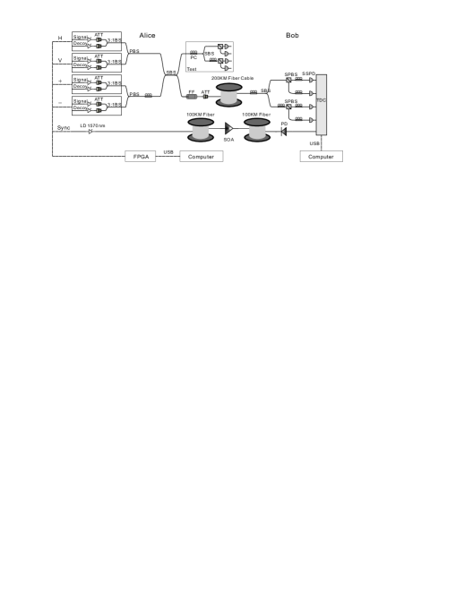
Our set-up is shown schematically in Figure 1. Two sides, Alice and Bob are linked by 200 km optical fiber. Decoy pulses of BB84 polarization states are sent to Bob through the optical fiber. They are detected at Bob’s side by superconducting single-photon detectors.
3.1 Source
We use the weak coherent light as our source. The main idea of the decoy-state method is to change intensities randomly among different values in sending out each pulses. Here we change the intensity of each pulses among 3 different values: 0, 0.2, 0.6, which are called vacuum pulse, decoy-pulse, and signal pulse, respectively. Alice’s probabilities of sending a vacuum pulse, a decoy pulse and a signal pulse are 1:1:2 . The experiment lasts for 3089 seconds.
As shown in Fig.1, the coherent light pulses in our experiment are produced by 8 diodes which are controlled by 4-bit random numbers random numbers. The first two bits of a random number determines whether to produce a vacuum pulse, a decoy pulse, or a signal pulse. In particular, if they are 00, none of the diode sends out any pulse, i.e., a vacuum pulse is produced; if they are 01, one of the 4 decoy diodes in the figure produces a decoy pulse; if they are 10 or 11, one of the 4 signal diodes in the figure produces a signal pulse. The last 2 bits of the 4-bit random number decides which of the 4 diodes is chosen to produce the pulse (If the first two bits are not 00 ). The light intensities are controlled by an attenuator after each diodes, 0.2 for the decoy pulse and 0.6 for the signal pulse. Each diodes will produce only one polarization from the 4 BB84 states, i.e., the horizontal, vertical, , . Polarization maintaining beam splitters (PMBS) are used to guide pulses from the decoy diode and the signal diode in the same polarization block into one PMBS. Two polarization maintaining polarization beam splitters are used to guide pulses from all diodes to one optical fiber. The fidelity of our polarization states is larger than . The Pulses produced by the laser diodes first passes through a polarization maintaining beam-splitter (BS), then a polarization beam splitter (PBS) and then combined by a single mode BS. These pulses are sent to Bob through the optical fiber of a 200 km long, in side the lab.
3.2 Detection
The circuit at Bob’s side is is a standard design of BB84 detection. Four super-conducting single-photon detectors are used to detect signals. These detectors are made by Scontel company in Russia. We have set the environmental temperature lower than 2.4k. The dark count rate of each detectors is smaller than 1 Hz and the detection efficiency of 3 of them is larger than 4%, one of them is larger than 3%.
3.3 Clock
The 40k Hz synchronization pulses are originated from the 320M Hz clock which drives a laser diode to produce synchronization pulses. In order to observe the detect the synchronization pulses at Bob’s side which is linked to Alice by 200 km optical fiber, a semiconductor optical amplifier is inserted at the point of 100 km, amplifying the intensity of optical pulses by 100 before transmission over the second half of the optical fiber. At Bob’s side, a photon-electrical detector is used to recover the synchronization pulses. Both the synchronization pulses and the electrical signal from the superconductor detector are sent to a time-to-digit convertor (TDC) which works as an ”economic local clock”.
4 Calculation of the final key
The secure final keys can be distilled with an imperfect source given the separate theoretical results from Ref. [5]. We regard the upper bound of the fraction of tagged bits as those raw bits generated by multiphoton pulses from Alice, or equivalently, the lower bound of the fraction of untagged bits as those raw bits generated by single-photon pulses from Alice. In Wang’s 3-intensity decoy-state protocol [12], Alice can randomly use 3 different intensities (average photon numbers) of each pulses (, , )as the vacuum pulses, decoy pulses and signal pulses. Alice produce the states by different intensities in Eq.1.
| (1) |
Here , , is a density operator, and (here we use the same notation in Ref. [12]. In the protocol, Bob records all the states which he observed his detector click. After Alice sent out all the pulses, Bob announced his record. Then they known the number of the counts , , which came from different intensities 0, , . , , are the pulse numbers of intensity , , which Alice sent out. The counting rates (the counting probability of Bob s detector whenever Alice sends out a state) of pulses of each intensities can be calculate , and , respectively. We denote (), () and () for the counting rates of those vacuum pulses, singlephoton pulses, and pulses from (). Asymptotically, the values of primed symbols here should be equal to those values of unprimed symbols. However, in an experiment the number of samples is finite; therefore they could be a bit different. The bound values of , can be determined by the following joint constraints equations:
| (2) |
where , , , , and to obtain the worst-case results [12]. Given these, one can calculate , , numerically.
In the experiment, Alice totally transmits about N pulses to Bob. After the transmission, Bob announces the pulse sequence numbers and basis information of received states. Then Alice broadcasts to Bob the actual state class information and basis information of the corresponding pulses. Alice and Bob can calculate the experimentally observed quantum bit error rate (QBER) values , of decoy states and signal states according to all the decoy bits and a small fraction of the signal bits, respectively. Since we exploit and from finite test bit, the statistical fluctuation should be consider to evaluate the error rate of the remaining bit.
| (3) |
is the proportion of the test bits for the phase-flip test in single states (decoy state). Then we can numerically calculate a tight lower bound of the counting rate of single-photon using Eq. (2). The next step is to estimate the fraction of single-photon and the QBER upper bound of single-photon . We use
| (4) |
to conservatively calculate of signal states and decoy states, respectively [12]. And of signal states and decoy states can be estimated by the following formula:
| (5) |
Here we consider the statistical fluctuations of the vacuum states to obtain the worst-case results.
Lastly, we can calculate the final key rates of signal states using the following formula [12]:
| (6) |
Here .
We consider the final key rate of the decoy states independently. During the above calculation, we have used the worst case results in every step for the security. Obviously, there are more economic methods for the calculation of final key rate of the decoy states. Here we have not considered the consumption of raw keys for the QBER test. Now we reconsider the key rate calculation of decoy states above. We assumed the worst case of and for calculating and , respectively. Although we do not exactly know the true value of , there must be one fixed value for both calculations. Therefore we can choose every possible value in the range of and use it to calculate , and the final key rate, and then pick out the smallest value as the lower bound of decoy states key rate. As the Fig. 3 in [26] , we set to calculate the lower bound of decoy states key rate. This economic calculation method can obtain a more tightened value of the lower bound, which is larger than the result using the simple calculation method above with the two-step worst-case assumption for values. We can calculate the final key rates of decoy states using the following formula with Equ. 3.
| (7) |
Half of the experimental data should be discarded due to the measurement basis mismatch in the BB84 protocol. Among the remaining half, the ratio are consumed for the phase-flip test and are consumed for the bit-flip test. Then we can calculate the final rate which exploit from single states and decoy states.
| (8) |
In the experiment, the pulse numbers ratio of the 3 intensities 0, and is 1:1:2 and the intensities of signal states and decoy states are fixed at and , respectively. The numbers of the counts from 0, anf are 3263, 77157 and 449467. We calculate the experimentally observed QBER values , of decoy states and signal states are , . The experiment lasts for seconds. We use for phase-flip test, and for bit-flip test. The experimental parameters and their corresponding values are listed in Table 1. After calculation, we obtain a final key rate of 11.8 bits/s for the signal states (intensity ) and a final key rate of 2.9 bits/s for the decoy states (intensity ).
| P | Value | P | Value | P | Value | P | Value |
|---|---|---|---|---|---|---|---|
| L | 200 km | ||||||
| 320 MHz | |||||||
| 0.0196 | |||||||
| 0.0404 | 11.8626Hz | 2.2972Hz |
5 Concluding remarks
In summary, with a superconducting detector, we have demonstrated a decoy-state QKD over 200km distance in polarization coding and optical fiber. In our experiment, the synchronization system is significantly simplified. In principle, the frequent synchronization pulses are not necessary in our set-up if one has a very precise local clock.
Acknowledgments
We acknowledge the financial support from the CAS, the National Fundamental Research Program of China under Grant No.2006CB921900, China Hi-Tech program grant No. 2006AA01Z420 and the NNSFC.