On Cross-correlations between Curvature and Isocurvature Perturbations during Inflation

Abstract:

We investigate the effects of couplings between curvature and isocurvature perturbations before and around horizon-crossings during cosmological inflation. We consider a generalized two-field inflation model, in which the non-canonical kinetic term allows us arbitrary sound speeds of curvature and isocurvature perturbations. By using the field-theoretical perturbative analysis, we calculate the cross-spectrum between curvature and isocurvature perturbations and the corrections to curvature and isocurvature power spectra due to the presence of couplings between them. Our analysis confirms previous results that the cross-correlations are generated and amplified when perturbations cross the horizons. Moreover, we find the cross-correlation, which was previously shown to be first-order in slow-roll parameter, can be enhanced when the sound speed of isocurvature perturbation is much smaller than that of the curvature perturbation. This is because in this case the isocurvature perturbation exits its horizon much earlier than the curvature perturbation and acts as a nearly constant source on the curvature perturbation.

1 Introduction

It is believed that the large-scale structure in our universe grows up from the primordial quantum fluctuations during a period of cosmological inflation (see e.g. [2] for a review). The predictions of inflation have been supported by current observational data [1].

The simplest model for inflation is based on the picture that a single scalar field rolls down its potential, making the universe inflate and also generating quantum fluctuations. However, various alternatives are investigated extensively, one of which is multi-field inflation models [3, 4, 5, 6, 7, 8, 9, 10, 11, 3, 12, 13, 15, 19, 20, 25, 26, 28, 16, 17, 18, 14, 21, 22, 27, 34]. The goal of the studies of multi-field models is two-fold. Firstly, many inflation models based on particle physics or string theory usually involve many scalar fields, which can also have non-canonical kinetic terms. Secondly, it has been clear that any detection of primordial non-gaussianity would rule out the simplest slow-roll single field inflation models. On the other hand, multiple field models provide us more possibilities and have been discussed extensively [40, 53, 41, 42, 55]. Thus, it is natural and important to study multi-field inflation models in details.

However, in the context of multi-field models, except for a few specific models, even the predictions for the spectra of primordial perturbations are a non-trivial task. The main reason is that, there are couplings between adiabatic mode and entropy mode(s), even at linear level. A well-known result is that the curvature (or adiabatic) perturbation can evolve on super-horizon scales in multi-field inflation whereas it is conserved in single-field inflation. This is due to that the entropy (isocurvature) perturbation modes act as a source term in the evolution equation for the curvature perturbation. This phenomena was first emphasized in [14]. The production of adiabatic and entropy modes for two-field models with a generic potential was studied in [15] where a decomposition into instantaneous adiabatic/entropy modes was firstly introduced. Multi-field models with non-canonical kinetic terms have been investigated in the slow-rolling approximation in [11, 12, 22], where the adiabatic/entropy decomposition technique was also extended in [19, 20] with non-canonical kinetic terms.

As has been stressed above, one of the difficulties in multi-field inflation researches is that, one cannot trace back the adiabatic mode to one of these scalar fields, and the entropy modes to remaining scalar fields. In general, all relevant scalar fields are mixed together to give one adiabatic modes and $N-1$ entropic modes. On the other hand, this is also the reason why we should expect cross-correlations between adiabatic and entropy modes [3, 4, 5]. However, in most of the previous works, quantum cross-correlations between adiabatic and entropy modes before and around horizon-crossing $\left\langle Q_{\sigma}Q_{s}\right\rangle_{\ast}$ are expected to be small, based on the observation that the cross-correlations are of order slow-rolling parameters before and around horizon-crossing. This cross-correlation has been studied analytically in [25] as a phenomena of oscillations between two perturbation modes and also been investigated in details in [26] with canonical kinetic term and in [27] with non-canonical kinetic term. Numerical studies were also presented in [28, 29].

The goal of this work is to study the cross-correlations in details. The analytic treatments in [25, 26, 27] are based on the “diagonalization” of the coupled system: time-dependent orthogonal matrices are introduced to abstract the approximately decoupled degrees of freedom which should be quantized. Indeed, this is the standard treatment to a coupled system. In this note, we take a slightly alternative approach — that is, we treat the couplings between adiabatic and entropy modes as “two-point” interactions, and use standard field theoretical perturbative methods to calculate the cross-correlation and also the corrections to adiabatic/entropy spectra themselves. More precisely, we split the full quadratic-order action into a “free” part in which adiabatic mode and entropy mode decouple with each other and a “two-point” interaction part, where the two-point couplings are treated as interaction vertices. Generally speaking, this approach supplies us a systematic perturbative procedure to study the coulings between adiabatic and entropy modes in details, especially in the cases where the “diagonalization” of the coupled system cannot be done easily or the “time-independence” of the diagonolization matrices is not a good approximation.

We consider a generalized two-field inflation model, as described in the next section. The prototype of this form of Lagrangian was proposed in [31, 35] and includes multi-field $k$-inflation [22, 40] and two-field DBI model [31, 32, 33, 41, 37, 43, 44] as special case and thus deserves detailed study. Actually, non-gaussianities in multi-field models with non-canonical kinetic terms have been extensively investigated in [31, 35, 40, 41, 42, 32, 33, 36, 37, 38, 39, 43, 44] (see also [50, 51, 52, 53, 54, 56, 55]). Although the main task in this note is not to study a complex multi-field model, this generalized Lagrangian can make our analysis of the cross-correlation in a more general background. Especially, the non-canonical kinetic term of our model allows us arbitrary sound speeds of adiabatic and entropy perturbations, which are essential for our following analysis. Our work can be viewed as generalization of the analysis in [25, 26, 27] to a general class of two-field models with non-canonical kinetic terms and arbitrary speeds of sound for adiabatic and entropy modes, $c_{a}\neq c_{e}$.

This paper is organized as follows. In the next section we introduce a generalized two-field inflation model, and describe the scalar perturbations of it. The third section is devoted to investigate the cross-correlations in detail, based on the field-theoretical perturbative approach. The last section is devoted to conclusion and discussion on the limitation and possible extension of this work.

2 Generalized Two-field Inflation Model

In this work, we consider a very general class of two-field inflation models with action of the form:

$${}S=\int d^{4}x\sqrt{-g}\left[\frac{1}{2}M_{\textrm{p}}^{2}R-P(X,Y,\phi^{I})\right]\,,$$ (1)

where $X\equiv X^{I}_{I}=G_{IJ}X^{IJ}$ and $Y\equiv X^{I}_{J}X^{J}_{I}$ with $X^{IJ}\equiv-\frac{1}{2}g^{\mu\nu}\partial_{\mu}\phi^{I}\partial_{\nu}\phi^{J}$, $G_{IJ}$ is the metric for the field space and $M_{\textrm{p}}\equiv 1/\sqrt{8\pi G}$ is the reduced Planck mass which we set to unity in the following. In two-field case, all higher order contractions among $X_{IJ}$’s can be expressed in terms of $X$ and $Y$, e.g.,

$$X^{I}_{J}X^{J}_{K}X^{K}_{I} =-\frac{X^{3}}{2}+\frac{3}{2}XY\,,$$

$$X^{I}_{J}X^{J}_{K}X^{K}_{L}X^{L}_{I} =-\frac{1}{2}X^{4}+X^{2}Y+\frac{1}{2}Y^{2}\,,$$

etc. The model (1) includes multi-field $k$-inflation and two-field DBI model as special cases. For example, in multi-DBI model the Lagrangian is $P=-\frac{1}{f(\phi^{I})}\left(\sqrt{\mathcal{D}}-1\right)-V(\phi^{I})$ with

$$\mathcal{D} \equiv\det\left(G^{I}_{J}-2fX^{I}_{J}\right)$$ (2)

$$=1-2fG_{IJ}X^{IJ}+4f^{2}X^{[I}_{I}X^{J]}_{J}-8f^{3}X^{[I}_{I}X^{J}_{J}X^{K]}_{K}+16f^{4}X^{[I}_{I}X^{J}_{J}X^{K}_{K}X^{L]}_{L}\,.$$

This expression for determinant $\mathcal{D}$ is general. In this work, we focus on two-field case, thus the last two terms exactly vanish, leaving us effectively $\mathcal{D}\equiv 1-2fG_{IJ}X^{IJ}+4f^{2}X^{[I}_{I}X^{J]}_{J}$. In terms of (1), this is just $\mathcal{D}=1-2fX+2f^{2}\left(X^{2}-Y\right)$.

This form of scalar-field Lagrangian in (1) is the most general Lagrangian for two-field models and thus deserves detailed investigations. The goal of choosing such a general Lagrangian in this note is not only because recent investigations on non-Gaussianities in multi-field are based on some similar Lagrangian [31, 35, 40, 41, 42, 32, 33, 36, 37, 38, 39, 43, 44], but also in order to see the effects on perturbations from the structure of the theory in a wider range. As we will see, the non-canonical kinetic term supplies us two different speeds of sound for adiabatic and entropy modes which we denote as $c_{a}$ and $c_{e}$ respectively, which are essential for our following analysis.

2.1 Background Equations of Motion

In this work, we investigate scalar perturbations around a flat FRW background, the background spacetime metric takes the form

$${}ds^{2}=-dt^{2}+a^{2}(t)\delta_{ij}dx^{i}dx^{j}\,,$$ (3)

where $a(t)$ is the scale-factor. The Friedmann equation and the continuity equation are

$$H^{2} \equiv\frac{\rho}{3}=\frac{1}{3}\left(2X^{IJ}P_{,\langle IJ\rangle}-P\right)\,,$$ (4)

$$\dot{\rho} =-3H(\rho+P)\,,$$

where and in what follows we denote $P_{,\langle IJ\rangle}\equiv\frac{\partial P}{\partial X^{IJ}}$, $P_{,\langle IJ\rangle\langle KL\rangle}\equiv\frac{\partial^{2}P}{\partial X^{IJ}\partial X^{KL}}$ etc. for short. In the above equations, all quantities are evaluated on the background. From the above two equations we can also get another convenient equation

$${}\dot{H}=-X^{IJ}P_{,\langle IJ\rangle}\,.$$ (5)

The background equations of motion for the scalar fields are

$$P_{,\langle IJ\rangle}\ddot{\phi}^{I}+\left(3HP_{,\langle IJ\rangle}+\dot{P}_{,\langle IJ\rangle}\right)\dot{\phi}^{I}-P_{,J}=0\,,$$ (6)

where $P_{,I}$ denotes derivative of $P$ with respect to $\phi^{I}$: $P_{,I}\equiv\frac{\partial P}{\partial\phi^{I}}$.

In this work, we investigate cosmological perturbations during an exponential inflation period. Thus, from (5) it is convenient to define a slow-roll parameter for the expansion rate

$${}\epsilon\equiv-\frac{d\ln H}{d\ln a}=-\frac{\dot{H}}{H^{2}}=\frac{P_{,\langle IJ\rangle}\dot{\phi}^{I}\dot{\phi}^{J}}{2H^{2}}\,.$$ (7)

In this note we do not go into details of solving the background equations of motion, but only assume that the structure of $P(X,Y,\phi^{I})$ and thus the background dynamical equations permit such an exponential expansion period.

2.2 Linear Perturbations

In this work we focus on the linear perturbations. In multi-field models, it is convenient to work in spatially-flat gauge, where the metric (scalar sector) is unperturbed as in (3), and the perturbation of the system is encoded in the perturbations of the scalar fields, which we denote $\delta\phi^{I}\equiv Q^{I}$ for short.

In multi-field inflation models, it is convenient to decompose perturbations into instantaneous adiabatic and entropy perturbations [15, 21]. This decomposition was firstly introduced in [15] in the study of two-field inflation with a generic potential, and was extended in [12, 19, 20] in two-field models with non-canonical kinetic terms. This decomposition technique was also generalized to non-linear perturbations [16] in the context of covariant non-linear formalism [17, 18].

The “adiabatic direction” corresponds to the direction of the “background inflaton velocity”, for model described in this work, it is

$$e^{I}_{\sigma}\equiv\frac{\dot{\phi}^{I}}{\sqrt{P_{,\langle JK\rangle}\dot{\phi}^{J}\dot{\phi}^{K}}}\equiv\frac{\dot{\phi}^{I}}{\dot{\sigma}}\,,$$ (8)

where $\dot{\sigma}$ is defined as

$${}\dot{\sigma}\equiv\sqrt{P_{,\langle JK\rangle}\dot{\phi}^{J}\dot{\phi}^{K}}\,,$$ (9)

which is the generalization of the background inflaton velocity. Actually $\dot{\sigma}$ is essentially a short notation and has nothing to do with any concrete field. Note that $\dot{\sigma}$ is related to the slow-roll parameter $\epsilon$ as $\dot{\sigma}^{2}=2H^{2}\epsilon$.

In this work we focus on two-field case. We introduce the entropy basis $e^{I}_{s}$ which is orthogonal to $e^{I}_{\sigma}$. The orthogonal condition can be defined as

$${}P_{,\langle IJ\rangle}e^{I}_{m}e^{J}_{n}\equiv\delta_{mn}\,,\qquad\qquad m,n=\sigma,s$$ (10)

Thus the scalar-field perturbation $Q^{I}$ can be decomposed into instantaneous adiabatic/entropy modes as:

$$Q^{I}\equiv e^{I}_{\sigma}Q_{\sigma}+e^{I}_{s}Q_{s}\,.$$ (11)

In spatially-flat gauge, the quadratic-order action for the perturbations of the model (1) can be calculated straightforwardly. After instantaneous adiabatic/entropy modes decomposition, up to total derivative terms, the second-order action for the scalar perturbations takes the form [31, 32, 35, 42]

$${}S_{2}\equiv\int dtd^{3}xa^{3}\left[\frac{1}{2}K_{mn}\dot{Q}^{m}\dot{Q}^{n}-\delta_{mn}\frac{1}{2a^{2}}\partial_{i}Q^{m}\partial_{i}Q^{n}+\Xi_{mn}\dot{Q}^{m}Q^{n}-\frac{1}{2}M_{mn}Q^{m}Q^{n}\right]\,,\\$$ (12)

with

$${}K_{mn} \equiv\delta_{mn}+\dot{\sigma}^{2}P_{,\langle IK\rangle\langle JL\rangle}e^{I}_{\sigma}e^{K}_{n}e^{J}_{\sigma}e^{L}_{m}\,,$$ (13)

$$=\delta_{mn}+\left(\frac{1}{c_{a}^{2}}-1\right)\delta_{\sigma m}\delta_{\sigma n}+\left(\frac{1}{c_{e}^{2}}-1\right)\left(\delta_{mn}-\delta_{\sigma m}\delta_{\sigma n}\right)\,,$$

$$\Xi_{mn} \equiv\mathcal{N}_{IJ}e_{m}^{I}e_{n}^{J}+\left(P_{\left\langle IJ\right\rangle}+2P_{\left\langle IK\right\rangle\left\langle JL\right\rangle}X^{KL}\right)e_{m}^{I}\dot{e}_{n}^{J}\,,$$

$$-M_{mn} =-\mathcal{M}_{IJ}e_{m}^{I}e_{n}^{J}+2\mathcal{N}_{IJ}\dot{e}_{m}^{I}e_{n}^{J}+\left(P_{\left\langle IJ\right\rangle}+2P_{\left\langle IK\right\rangle\left\langle JL\right\rangle}X^{KL}\right)\dot{e}_{m}^{I}\dot{e}_{n}^{J}\,,\qquad\quad(m,n=\sigma,s)$$

where

$$\mathcal{N}_{IJ} \equiv\dot{\phi}^{K}P_{\left\langle KI\right\rangle,J}-\frac{2}{H}X^{KL}X^{NM}P_{\left\langle NI\right\rangle\left\langle KL\right\rangle}P_{\left\langle MJ\right\rangle}\,,$$ (14)

$$-\mathcal{M}_{IJ} \equiv P_{,IJ}+\left(X^{MN}P_{\left\langle MN\right\rangle}+2X^{MN}X^{PQ}P_{\left\langle MN\right\rangle\left\langle PQ\right\rangle}-3H^{2}\right)\frac{X^{KL}}{H^{2}}P_{\left\langle KI\right\rangle}P_{\left\langle LJ\right\rangle}$$

$$\qquad+\frac{1}{H}\left(P_{,I}-2X^{MN}P_{\left\langle MN\right\rangle,I}\right)P_{\left\langle KJ\right\rangle}\dot{\phi}^{K}+\frac{1}{a^{3}}\frac{d}{dt}\left(\frac{a^{3}}{H}X^{KL}P_{\left\langle KI\right\rangle}P_{\left\langle LJ\right\rangle}\right)\,.$$

In (13) we introduce

$${}c_{a}^{2} \equiv\frac{P_{,X}+2XP_{,Y}}{P_{,X}+2X\left(P_{,XX}+4XP_{,XY}+3P_{,Y}+4X^{2}P_{,YY}\right)}\,,$$ (15)

$$c_{e}^{2} \equiv\frac{P_{,X}}{P_{,X}+2XP_{,Y}}\,,$$

which are the propagation speeds of the adiabatic mode and entropy mode respectively. From (13), the kinetic term $K_{mn}\dot{Q}^{m}\dot{Q}^{n}$ has been diagonalized, as a result of adiabatic/entropy decomposition.

For our purpose in this work, the different speeds of sound for adiabatic and entropy modes are essential for the investigation of cross-correlations. Actually in multi-field models, it is generic fact that $c_{a}\neq c_{e}$ which was firstly point out apparently in [23, 24] in the investigation of brane inflation model. In multiple $k$-inflation with Lagrangian of the form $P(X,\phi^{I})$, the adiabatic mode propagate with sound speed $c_{s}$ while entropy modes propagate with the speed of light [22, 40]. While subsequently in [31, 35], it was shown that in multi-DBI models, the adiabatic mode and entropy modes propagate with the same speed of sound. Now it becomes clear that, in multi-field inflationary models, adiabatic mode and entropic modes in general propagate with different speeds of sound $c_{a}$ and $c_{e}$, which depend on the structure of specific theory [31, 35] (see also [35, 32, 57, 58, 51, 40, 41] for extensive investigations on general multi-field models with different $c_{a}$ and $c_{e}$).

It is now convenient to introduce the canonically normalized variables

$$\tilde{Q}_{\sigma}=\frac{a}{c_{a}}Q_{\sigma}\,,\qquad\tilde{Q}_{s}=\frac{a}{c_{e}}Q_{s}\,.$$ (16)

After straightforward but tedious calculations, the quadratic action for $\tilde{Q}_{\sigma}$ and $\tilde{Q}_{s}$ (after using conformal time $\eta$ defined by $dt=ad\eta$ and up to total derivative terms) takes the form:

$${}S_{2}[\tilde{Q}_{\sigma},\tilde{Q}_{s}] =\int d\eta d^{3}x\,\frac{1}{2}\left[\tilde{Q}_{\sigma}^{\prime 2}-c_{a}^{2}\left(\partial\tilde{Q}_{\sigma}\right)^{2}+\frac{z^{\prime\prime}}{z}\tilde{Q}_{\sigma}^{2}+\tilde{Q}_{s}^{\prime 2}-c_{e}^{2}\left(\partial\tilde{Q}_{s}\right)^{2}+\left(\frac{\alpha^{\prime\prime}}{\alpha}-a^{2}\mu_{s}^{2}\right)\tilde{Q}_{s}^{2}\right.$$ (17)

$$\qquad\qquad\qquad\qquad\left.-2\mathcal{H}\xi\,\tilde{Q}_{\sigma}^{\prime}\tilde{Q}_{s}+2\frac{z^{\prime}\mathcal{H}\xi}{z}\,\tilde{Q}_{\sigma}\tilde{Q}_{s}\right]\,,$$

where

$${}\xi =\frac{1}{\sqrt{2\epsilon}\sqrt{P_{1}}c_{a}}\left[(1+c_{a}^{2})\frac{P_{,s}}{H^{2}}-2\epsilon c_{a}^{2}P_{,1s}\right]\,,$$ (18)

$$z =a\frac{\dot{\sigma}}{c_{a}H}\,,$$

$$\alpha =a\sqrt{P_{1}}\,,$$

$$\mu_{s}^{2} =-\frac{P_{,ss}}{P_{1}}+\frac{\dot{\sigma}^{2}\tilde{R}}{2P_{1}}-\frac{P_{,s}^{2}}{c_{a}^{2}\dot{\sigma}^{2}P_{1}^{2}}+\frac{2P_{1s}P_{,s}}{P_{1}^{2}}\,,$$

with

$$P_{,s} =P_{,I}e^{I}_{s}\sqrt{P_{1}}\,c_{e}\,,\qquad P_{,1s}=(\partial_{I}P_{1})e^{I}_{s}\sqrt{P_{1}}\,c_{\textrm{e}}\,,\qquad P_{,ss}=c_{e}^{2}P_{1}\left(\mathcal{D}_{I}\mathcal{D}_{J}P\right)e^{I}_{s}e^{J}_{s}\,,$$ (19)

$$P_{1} \equiv P_{,X}+2XP_{,Y}\,,$$

and $\tilde{R}$ is the Ricci scalar of field space metric $G_{IJ}$, $\mathcal{D}_{I}$ is the covariant derivative associated to $G_{IJ}$ (i.e. $\mathcal{D}_{I}\mathcal{D}_{J}P\equiv P_{,IJ}-\Gamma^{K}_{IJ}P_{,K}$). Note that these various parameters are evaluated on the background. In general, the time-dependence of these various parameters are complicated. In this note, in order to proceed, we introduce several slow-varying parameters:

$${}\eta_{\epsilon}\equiv\frac{\textrm{d}\ln\epsilon}{\textrm{d}\ln a}\,,\qquad s_{a}\equiv\frac{\textrm{d}\ln c_{a}}{\textrm{d}\ln a}\,,\qquad s_{e}\equiv\frac{\textrm{d}\ln c_{e}}{\textrm{d}\ln a}\,,\qquad\eta_{p}\equiv\frac{\textrm{d}\ln P_{1}}{\textrm{d}\ln a}\,,\qquad\eta_{\xi}\equiv\frac{\textrm{d}\ln\xi}{\textrm{d}\ln a}$$ (20)

where $a$ is the scale-factor.

In canonical quantization procedure, the quantum fields are decomposed as

$${}\tilde{Q}_{\sigma}(\bm{k},\eta)\equiv a_{\bm{k}}u_{\sigma}(k,\eta)+a^{{\dagger}}_{-\bm{k}}u^{\ast}_{\sigma}(k,\eta)\,,\qquad\qquad\tilde{Q}_{s}(\bm{k},\eta)\equiv b_{\bm{k}}u_{s}(k,\eta)+b^{{\dagger}}_{-\bm{k}}u^{\ast}_{s}(k,\eta)\,,$$ (21)

The equations of motion for the mode functions $u_{\sigma}$ and $u_{s}$ can be get from varying (17):

$${}u^{\prime\prime}_{\sigma}+\left(c_{a}^{2}k^{2}-\frac{z^{\prime\prime}}{z}\right)u_{\sigma}-\mathcal{H}\xi u^{\prime}_{s}-\frac{(z\mathcal{H}\xi)^{\prime}}{z}u_{s} =0\,,$$ (22)

$$u^{\prime\prime}_{s}+\left(c_{e}^{2}k^{2}-\frac{\alpha^{\prime\prime}}{\alpha}+a^{2}\mu_{s}^{2}\right)u_{s}+\mathcal{H}\xi u^{\prime}_{\sigma}-\frac{z^{\prime}\mathcal{H}\xi}{z}u_{\sigma} =0\,,$$

These two equations form a closed system for the scalar perturbations.

3 Perturbative Analysis

As described in the Introduction, the idea in this paper is to treat the coupling between adiabatic and entropy modes as “two-point” interaction vertices, and to use field theoretical perturbative approaches to evaluate the cross-correlations.

3.1 Interaction Hamiltonian

The first line in (17) describes a decoupled two-field system, where the two decoupled modes can be quantized independently. While the second-line can be identified as the “two-point cross-interaction vertices”:

$$S_{c}[\tilde{Q}_{\sigma},\tilde{Q}_{s}]=\int d\eta d^{3}x\,\left(-\mathcal{H}\xi\,\tilde{Q}_{\sigma}^{\prime}\tilde{Q}_{s}+\frac{z^{\prime}\mathcal{H}\xi}{z}\,\tilde{Q}_{\sigma}\tilde{Q}_{s}\right)\,,$$ (23)

where the dimensionless cross-coupling $\xi$ is given in (18). In the operator formalism of quantization, interaction Hamiltonian is needed. The Hamiltonian density which is defined by $\mathcal{H}\equiv\pi_{a}Q^{\prime}_{a}-\mathcal{L}$ can be split into two parts: $\mathcal{H}\equiv\mathcal{H}_{0}+\mathcal{H}_{c}$, with

$${}\mathcal{H}_{0} \equiv\frac{1}{2}\pi_{\sigma}^{2}+\frac{1}{2}c_{a}^{2}\left(\partial\tilde{Q}_{\sigma}\right)^{2}-\frac{z^{\prime\prime}}{2z}\tilde{Q}_{\sigma}^{2}+\frac{1}{2}\pi_{s}^{2}+\frac{1}{2}c_{e}^{2}\left(\partial\tilde{Q}_{s}\right)^{2}-\frac{1}{2}\left(\frac{\alpha^{\prime\prime}}{\alpha}-a^{2}\mu_{s}^{2}-\mathcal{H}^{2}\xi^{2}\right)\tilde{Q}_{s}^{2}\,,$$ (24)

$$\mathcal{H}_{c} \equiv\mathcal{H}\xi\,\pi_{\sigma}\tilde{Q}_{s}-\frac{z^{\prime}\mathcal{H}\xi}{z}\tilde{Q}_{\sigma}\tilde{Q}_{s}\,,$$

where $\mathcal{H}_{0}$ describes decoupled system while $\mathcal{H}_{c}$ describes the cross interactions. From $\mathcal{H}_{0}$, the free-theory canonical momenta are (in interaction picture) are related with time-derivatives of the fields as

$$\tilde{Q}^{\prime}_{\sigma}\equiv\frac{\partial\mathcal{H}_{0}}{\partial\pi_{\sigma}}=\pi_{\sigma}\,,\qquad\tilde{Q}^{\prime}_{s}\equiv\frac{\partial\mathcal{H}_{0}}{\partial\pi_{s}}=\pi_{s}\,,$$ (25)

thus in the interaction picture, the cross-interaction vertices can be written in terms of $\tilde{Q}_{m}$ and $\tilde{Q}^{\prime}_{m}$ as

$${}\mathcal{H}_{c}=\mathcal{H}\xi\,\tilde{Q}^{\prime}_{\sigma}\tilde{Q}_{s}-\frac{z^{\prime}\mathcal{H}\xi}{z}\tilde{Q}_{\sigma}\tilde{Q}_{s}\,.$$ (26)

Since $\tilde{Q}_{\sigma}$ and $\tilde{Q}_{s}$ are the canonical variables for quantization, the corresponding mode functions in (21) satisfy the decoupled (“free-theory”) equations of motion:

$${}u^{\prime\prime}_{\sigma}+\left(c_{a}^{2}k^{2}-\frac{z^{\prime\prime}}{z}\right)u_{\sigma} =0\,,$$ (27)

$$u^{\prime\prime}_{s}+\left(c_{e}^{2}k^{2}-\frac{\alpha^{\prime\prime}}{\alpha}+a^{2}\mu_{s}^{2}\right)u_{s} =0\,.$$

Up to the first-order in slow-varying parameters, the mode solutions with proper initial conditions are (See Appendix D for details)

$${}u_{\sigma}\left(\eta,k\right) =\frac{\sqrt{\pi}}{2}\left(1+\frac{s_{a}}{2}\right)e^{\frac{i\pi}{2}\left(\nu_{\sigma}+\frac{1}{2}\right)}\sqrt{-\eta}H^{(1)}_{\nu_{\sigma}}\left((1+s_{a})x\right)\,,$$ (28)

$$u_{s}\left(\eta,k\right) =\frac{\sqrt{\pi}}{2}\left(1+\frac{s_{e}}{2}\right)e^{\frac{i\pi}{2}\left(\nu_{s}+\frac{1}{2}\right)}\sqrt{-\eta}H_{\nu_{s}}^{\left(1\right)}\left(\left(1+s_{e}\right)y\right)\,,$$

with $x\equiv-c_{a}k\eta$ and $y\equiv-c_{e}k\eta$, and

$${}\nu_{\sigma} =\frac{3}{2}+\frac{1}{2}\left(2\epsilon+\eta_{\epsilon}+s_{a}\right)\,,$$ (29)

$$\nu_{s} =\tilde{\nu}+\eta_{p}\frac{3}{4\tilde{\nu}}+s_{e}\tilde{\nu}+\epsilon\left(\tilde{\nu}-\frac{3}{4\tilde{\nu}}\right)\,,$$

where $\tilde{\nu}=\sqrt{\frac{9}{4}-\frac{\mu_{s}^{2}}{H^{2}}}$, $H^{(1)}$ is the Hankel function of the first kind.

The “decoupled” two-point functions for $\tilde{Q}_{\sigma}$ and $\tilde{Q}_{s}$ are defined as

$${}\left\langle\tilde{Q}_{\sigma}(\bm{k}_{1},\eta_{1})\tilde{Q}_{\sigma}(\bm{k}_{2},\eta_{2})\right\rangle^{(0)}=(2\pi)^{3}\delta^{2}(\bm{k}_{1}+\bm{k}_{2})\tilde{G}_{k_{1}}(\eta_{1},\eta_{2})\,,$$ (30)

$$\left\langle\tilde{Q}_{s}(\bm{k}_{1},\eta_{1})\tilde{Q}_{s}(\bm{k}_{2},\eta_{2})\right\rangle^{(0)}=(2\pi)^{3}\delta^{2}(\bm{k}_{1}+\bm{k}_{2})\tilde{F}_{k_{1}}(\eta_{1},\eta_{2})\,,$$

where the supercript “⁽⁰⁾” means in evaluating the above expressions the coupling between adiabatic and entropy modes are neglected, and

$${}\tilde{G}_{k}(\eta_{1},\eta_{2})\equiv u_{\sigma}(\eta_{1},k)u^{\ast}_{\sigma}(\eta_{2},k)\,,\qquad\qquad\tilde{F}_{k}(\eta_{1},\eta_{2})\equiv u_{s}(\eta_{1},k)u^{\ast}_{s}(\eta_{2},k)\,,$$ (31)

where $u_{\sigma}$, $u_{s}$ are given in (28), and ^∗ denotes complex conjugate.

In comoving gauge, the perturbation $Q_{\sigma}$ is directly related to the three-dimensional curvature of the constant time space-like hypersurfaces. This gives the gauge-invariant quantity referred to the well-known “comoving curvature perturbation”:

$${}\mathcal{R}\equiv\frac{H}{\dot{\sigma}}Q_{\sigma}\,,$$ (32)

where $\dot{\sigma}$ is defined in (9). The entropy perturbation $Q_{s}$ is automatically gauge-invariant by construction. In practise, it is also convenient to introduce a renormalized “isocurvature perturbation” defined by

$${}\mathcal{S}\equiv\frac{H}{\dot{\sigma}}Q_{s}\,.$$ (33)

It is thus well-known result that the power spectra for curvature perturbation and isocurvature perturbation around their respective sound horizon-crossings are (up to the first-order in slow-varying parameters)

$${}\mathcal{P}_{\mathcal{R}}^{(0)}(x_{\ast}) =\left.\bar{\mathcal{P}}_{\mathcal{R}}\left(1-2\epsilon-2s_{a}\right)F_{\nu_{\sigma}}\left(\left(1+s_{a}\right)x\right)\right|_{{c_{a}k}/{aH}=1}\,,$$ (34)

$$\mathcal{P}_{\mathcal{S}}^{(0)}(y_{\ast}) =\left.\bar{\mathcal{P}}_{\mathcal{S}}\left(1-2\epsilon-2s_{e}\right)F_{\nu_{s}}\left(\left(1+s_{e}\right)y\right)\right|_{{c_{e}k}/{aH}=1}\,,$$

respectively, where the various parameters are defined in (20) and $\bar{\mathcal{P}}_{\mathcal{R}}\equiv\left(\frac{H}{2\pi}\right)^{2}\frac{1}{2\epsilon c_{a}}$ and $\bar{\mathcal{P}}_{\mathcal{S}}\equiv\left(\frac{H}{2\pi}\right)^{2}\frac{1}{2\epsilon c_{e}}$ are asymptotic values for the power spectra on superhorizon scales, and

$$F_{\nu}(x)\equiv\frac{\pi}{2}x^{3}\left|H_{\nu}^{\left(1\right)}\left(x\right)\right|^{2}\,.$$ (35)

In (34), quantities on the right-hand-side of the equations are evaluated at the time of adiabatic or entropy sound horizon-crossings, i.e. ${c_{a}k}/{aH}=1$ or ${c_{e}k}/{aH}=1$, respectively. In general since $c_{a}\neq c_{e}$, adiabatic and entropy modes cross their respective sound horizons at different times. For later convenience, we introduce $x\equiv-c_{a}k\eta$ and $y\equiv-c_{e}k\eta$, and in (34), $x_{\ast}$ and $y_{\ast}$ are their respective values around sound horizon-crossings, up to the first-order in slow-roll parameters which read

$$x_{\ast} \equiv\left.-c_{a}k\eta\right|_{c_{a}k/aH=1}\simeq 1+\left.\epsilon\right|_{c_{a}k/aH=1}\,,$$ (36)

$$y_{\ast} \equiv\left.-c_{e}k\eta\right|_{c_{e}k/aH=1}\simeq 1+\left.\epsilon\right|_{c_{e}k/aH=1}\,,$$

where $\epsilon$ is the slow-roll parameter define in (7).

In the above derivation, $\mu_{s}^{2}/H^{2}$ and thus $3-2\nu_{s}$ are not supposed to be small. While in the following discussion, we assume that $3-2\nu_{s}$ is of order $\sim\mathcal{O}(\epsilon)$. Actually if the perturbation mode has an effective mass comparable to the Hubble scale $H$, its quantum fluctuations on wavelengths larger than the effective Compton wavelength would be suppressed, then the system can be described effectively by a single-field.

3.2 Cross-correlations

Now we are at the point to evaluate the cross-power spectrum. As has been stressed, the idea is treat the cross-coupling terms as interaction vertices. From (26), there are two types of two-point cross-interaction vertices, as depicted in fig.1.

Figure 1: Diagrammatic representations for cross-correlation vertices. Black line denotes adiabatic mode and dashed line denotes entropy mode. A “$\otimes$” denotes cross-interaction vertex. There are two type of cross-interaction vertices. A black dot denotes temporal derivative.

In cosmological context, perturbative calculations of the correlation functions are based on the “in-in” formalism (see Appendix A for a brief review). The leading-order cross-correlation involves one cross-interaction vertex (see fig.1):

$${}\left\langle\tilde{Q}_{\sigma}\left(\eta,\bm{k}_{1}\right)\tilde{Q}_{s}\left(\eta,\bm{k}_{2}\right)\right\rangle =-2\Re\,i\int_{-\infty}^{\eta}d\eta^{\prime}\left\langle\tilde{Q}_{\sigma}\left(\eta,\bm{k}_{1}\right)\tilde{Q}_{s}\left(\eta,\bm{k}_{2}\right)H_{c}\left(\eta^{\prime}\right)\right\rangle$$ (37)

$$=-2\Re\,i\int_{-\infty}^{\eta}d\eta^{\prime}\left[\mathcal{H}\xi\left(\eta^{\prime}\right)\frac{d}{d\eta^{\prime}}\tilde{G}_{k_{1}}\left(\eta,\eta^{\prime}\right)\tilde{F}_{k_{1}}\left(\eta,\eta^{\prime}\right)-\frac{\mathcal{H}z^{\prime}\xi\left(\eta^{\prime}\right)}{z}\tilde{G}_{k_{1}}\left(\eta,\eta^{\prime}\right)\tilde{F}_{k_{1}}\left(\eta,\eta^{\prime}\right)\right]\,.$$

where $\tilde{G}$, $\tilde{F}$ are defined in (30). From now on, we take the massless limit (i.e. $\nu_{\sigma}=\nu_{s}=\frac{3}{2}$) for the decoupled two-point Green’s functions $\tilde{G}$ and $\tilde{F}$ defined in (28)-(31) and also treat $H$ etc. as constant in evaluating the cross-correlation and the corrections to adiabatic/entropy spectra. This is because not only that the exact Green’s functions are rather difficult to deal with analytically, but also that the differences between using the massless Green’s function and using the exact Green’s functions for our calculations are higher-order in slow-roll parameters. More precisely, we thus treat $\xi$ on the same footing as the other slow-varying parameters, and identifies terms such as $\epsilon\xi$ as higher-order quantities which can be neglected. At the end of our calculations, the time-dependence of various parameters such as $H$ should be taken into account in order to get the correct tilts of the spectra.

The cross-power spectrum for $Q_{\sigma}$ and $Q_{s}$ can be defined as

$$\left\langle Q_{\sigma}\left(\eta,\bm{k}_{1}\right)Q_{s}\left(\eta,\bm{k}_{2}\right)\right\rangle=\frac{c_{a}c_{e}}{a^{2}(\eta)}\left\langle\tilde{Q}_{\sigma}\left(\eta,\bm{k}_{1}\right)\tilde{Q}_{s}\left(\eta,\bm{k}_{2}\right)\right\rangle\equiv\left(2\pi\right)^{3}\delta^{3}\left(\bm{k}_{1}+\bm{k}_{2}\right)C_{\sigma s}\left(\eta,k_{1}\right)\,,$$ (38)

From (37) and (28)-(31), after a straightforward calculation, $C_{\sigma s}$ can be written in the form

$${}C_{\sigma s}(\eta,k)=\frac{H^{2}}{2c_{a}k^{3}}\,\xi\,\Gamma_{c}(x,\lambda)\,,$$ (39)

with $x\equiv-c_{a}k\eta$ again and

$$\lambda\equiv\frac{c_{e}}{c_{a}}\,,$$ (40)

is the ratio of sound speeds of entropy and adiabatic modes, and

$${}\Gamma_{c}(x,\lambda) \equiv\frac{\left(1+\lambda\right)}{2\lambda^{2}}\Big{\{}2-x\left[2\sin\left(\left(1+\lambda\right)x\right)\textrm{Ci}\left(\left(1+\lambda\right)x\right)+\cos\left(\left(1+\lambda\right)x\right)\left(\pi-2\textrm{Si}\left(\left(1+\lambda\right)x\right)\right)\right]$$ (41)

$$\qquad-\frac{1-\lambda x^{2}}{1+\lambda}\left[2\cos\left(\left(1+\lambda\right)x\right)\textrm{Ci}\left(\left(1+\lambda\right)x\right)-\sin\left(\left(1+\lambda\right)x\right)\left(\pi-2\textrm{Si}\left(\left(1+\lambda\right)x\right)\right)\right]\Big{\}}\,,$$

Here we keep the $\eta$-dependence in the expression for $\Gamma_{c}$ explicitly. It is not only because that there are inflation models where the perturbation spectra evolves quickly even after horizon crossing and never reaches the asymptotic values on superhorizon scales ($x\rightarrow 0$), but also allows us a more precise estimate of the spectra around the horizon crossing. It is also interesting to note that the cross-power spectrum depends explicitly on the ratio of the sound speeds for adiabatic and entropy modes $\lambda=c_{e}/c_{a}$. Especially, the factor $\Gamma_{c}$ depends only on the ratio $\lambda$, while not on $c_{a}$ or $c_{e}$ themselves. The dimensionless cross-power spectrum between $\mathcal{R}$ and $\mathcal{S}$ is given by

$${}\mathcal{C}_{\mathcal{R}\mathcal{S}}(\eta,k) \equiv\frac{k^{3}}{2\pi^{2}}\left(\frac{H}{\dot{\sigma}}\right)^{2}C_{\sigma s}(\eta,k)=\bar{\mathcal{P}}_{\mathcal{R}}\,\xi\,\Gamma_{c}(x,\lambda)\,,$$ (42)

where $\bar{\mathcal{P}}_{\mathcal{R}}\equiv\frac{1}{2\epsilon c_{a}}\left(\frac{H}{2\pi}\right)^{2}$ is asymptotic value for the dimensionless power spectrum for the comoving curvature perturbation on superhorizon scales as before.

(39)-(41) and (42) are one of the main results in this note. The key point is that, at leading-order the cross-power spectrum is of order $\sim\xi$, however its amplitude is determined by the factor $\Gamma_{c}(x,\lambda)$. The dependence of $\Gamma_{c}$ on $x$ and $\lambda$ is depicted in fig.2.

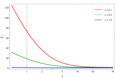
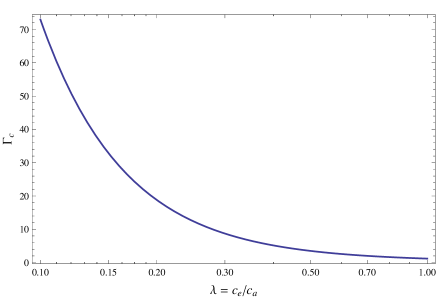
Figure 2: $\Gamma_{c}$ as function of $x$ (left) and as function of $\lambda$ evaluated around adiabatic sound horizon-crossing at $x\approx 1$ (right).

Two comments are in order:

• From the left panel in fig.2, when modes are deep inside the horizons, $\Gamma_{c}\ll 1$ and the cross-spectrum are indeed small. This confirms previous result that cross-correlations among different perturbation modes are always negligible when modes are deep in side their respective sound-horizons [25, 26, 27], since there the system reduces to a collection of weakly-coupled oscillators. However, as firstly pointed out in [25], as long as the modes get closed to the horizon(s), the couplings and thus cross-correlations among different modes become more and more important, and the cross-correlations are generated when modes cross their horizons. Our analysis also confirms this result. As depicted in the left panel in fig.2, when modes get closed to the horizon, $\Gamma_{c}$ starts to increase, and its amplitude is determined by $\lambda=c_{e}/c_{a}$, i.e. the ratio of the sound speeds of isocurvature and curvature perturbations.

• It is more interesting to note from the right panel in fig.2 that, the value of $\Gamma_{c}$ and thus the cross-correlation (around adiabatic sound horizon-crossing) can be enhanced by small $\lambda$, i.e for models with $c_{e}\ll c_{a}$. This phenomenon can be understood intuitively. As we know, the smaller the sound speed is, the earlier the corresponding perturbation mode crosses its sound horizon. The small $c_{e}/c_{a}$ ratio implies that the isocurvature perturbation exits its sound horizon much earlier before the curvature perturbation exits its sound horizon. Thus in the process when curvature perturbation gets closed to the adiabatic horizon, the isocurvature perturbation is already well outside its entropic horizon and behaves as a nearly constant (rather than highly oscillating) background, which acts as a nearly constant source on the curvature perturbation. More precisely, the smaller $\lambda$ is, the longer that the isocurvature perturbation behaves as a source on the curvature perturbation, and the more significant this “accumulative” effect is. This fact causes the amplifications of both cross-spectrum between curvature and isocurvature modes and also the corrections to the spectra of curvature and isocurvature perturbations by small $\lambda$, as we will show in the following subsection.

3.3 Corrections to Spectra of Curvature and Isocurvature Perturbations

Now we would like to investigate the leading-order corrections to the power spectra of curvature and isocurvature perturbations, due to the presence of the cross-interactions. It is interesting to note that the leading-order corrections to $P_{\sigma}$ and $P_{s}$ from the cross-interaction vertices involve two cross-interaction vertices and thus are of $\sim\xi^{2}$, as depicted in fig.3.

Figure 3: Diagrammatic representations of the leading-order corrections to $P_{\sigma}$ and $P_{s}$. Recall that there are two types of cross-interaction vertices, and thus there are actually four different contributions, which we do not show here explicitly.

The leading-order correction to the adiabatic power spectrum can be denoted as

$$\left\langle Q_{\sigma}\left(\eta,\bm{k}_{1}\right)Q_{\sigma}\left(\eta,\bm{k}_{2}\right)\right\rangle^{(2)}\equiv\left(2\pi\right)^{3}\delta^{3}\left(\bm{k}_{1}+\bm{k}_{2}\right)P_{\sigma}^{(2)}\left(\eta,k_{1}\right)\,,$$ (43)

here a superscript “⁽²⁾” denotes that the contribution involves two cross-interaction vertices, and

$${}P_{\sigma}^{(2)}\left(\eta,k_{1}\right)= -4\xi^{2}\times\Re\int_{-\infty}^{\eta}d\eta_{1}\int_{-\infty}^{\eta_{1}}d\eta_{2}F_{k_{1}}\left(\eta_{1},\eta_{2}\right)$$ (44)

$$\qquad\Big{[}\frac{1}{\eta_{1}\eta_{2}}\frac{d}{d\eta_{1}}G_{k_{1}}\left(\eta,\eta_{1}\right)\frac{d}{d\eta_{2}}G_{k_{1}}\left(\eta,\eta_{2}\right)+\frac{1}{\eta_{1}\eta_{2}^{2}}\frac{d}{d\eta_{1}}G_{k_{1}}\left(\eta,\eta_{1}\right)G_{k_{1}}\left(\eta,\eta_{2}\right)$$

$$\qquad+\frac{1}{\eta_{1}^{2}\eta_{2}}G_{k_{1}}\left(\eta,\eta_{1}\right)\frac{d}{d\eta_{2}}G_{k_{1}}\left(\eta,\eta_{2}\right)+\frac{1}{\eta_{1}^{2}\eta_{2}^{2}}G_{k_{1}}\left(\eta,\eta_{1}\right)G_{k_{1}}\left(\eta,\eta_{2}\right)\Big{]}$$

$$+2\xi^{2}\int_{-\infty}^{\eta}d\eta_{1}\int_{-\infty}^{\eta}d\eta_{2}F_{k_{1}}\left(\eta_{1},\eta_{2}\right)$$

$$\qquad\times\Big{[}\frac{1}{\eta_{1}\eta_{2}}\frac{d}{d\eta_{1}}G_{k_{1}}\left(\eta_{1},\eta\right)\frac{d}{d\eta_{2}}G_{k_{1}}\left(\eta,\eta_{2}\right)+\frac{1}{\eta_{1}\eta_{2}^{2}}\frac{d}{d\eta_{1}}G_{k_{1}}\left(\eta_{1},\eta\right)G_{k_{1}}\left(\eta,\eta_{2}\right)$$

$$\qquad+\frac{1}{\eta_{1}^{2}\eta_{2}}G_{k_{1}}\left(\eta_{1},\eta\right)\frac{d}{d\eta_{2}}G_{k_{1}}\left(\eta,\eta_{2}\right)+\frac{1}{\eta_{1}^{2}\eta_{2}^{2}}G_{k_{1}}\left(\eta_{1},\eta\right)G_{k_{1}}\left(\eta,\eta_{2}\right)\Big{]}\,.$$

Here $G_{k}(\eta_{1},\eta_{2})\equiv\frac{c_{a}^{2}}{a(\eta_{1})a(\eta_{2})}\tilde{G}_{k}(\eta_{1},\eta_{2})$ and $F_{k}(\eta_{1},\eta_{2})\equiv\frac{c_{e}^{2}}{a(\eta_{1})a(\eta_{2})}\tilde{F}_{k}(\eta_{1},\eta_{2})$. After a straightforward calculation, $P_{\sigma}^{(2)}$ can be written in the following form

$${}P_{\sigma}^{(2)}=\bar{P}_{\sigma}\xi^{2}\,\Gamma_{\sigma}\left(x,\lambda\right)\,,$$ (45)

where $\bar{P}_{\sigma}\equiv\frac{H^{2}}{2c_{a}k^{3}}$, and

$$\Gamma_{\sigma}\left(x,\lambda\right)= \frac{1}{8\lambda^{3}x}\left\{x\left[-16(\lambda+1)\text{Ci}\left(2x\right)\cos\left(2x\right)+8(\lambda+1)\left(\pi-2\text{Si}\left(2x\right)\right)\sin\left(2x\right)+16\lambda+\pi^{2}+24\right]\right.$$ (46)

$$+x^{2}\left[16(\lambda+1)\text{Ci}\left(2x\right)\left(x\cos\left(2x\right)-2\sin\left(2x\right)\right)+x\left(\pi^{2}-8(\lambda+1)\left(\pi-2\text{Si}\left(2x\right)\right)\sin\left(2x\right)\right)\right.$$

$$\qquad\quad\left.-16(\lambda+1)\left(\pi-2\text{Si}\left(2x\right)\right)\cos\left(2x\right)-4\pi\cos\left(x(\lambda+1)\right)\right]$$

$$+4\left(x^{3}+x\right)\text{Ci}^{2}\left((\lambda+1)x\right)-8\left(x^{2}+1\right)\text{Ci}\left((\lambda+1)x\right)\sin\left(x(\lambda+1)\right)+4\left(x^{3}+x\right)\text{Si}^{2}\left((\lambda+1)x\right)$$

$$\left.+4\left(x^{2}+1\right)\text{Si}\left((\lambda+1)x\right)\left[2\cos\left(x(\lambda+1)\right)-\pi x\right]-4\pi\cos\left(x(\lambda+1)\right)\right\}+\frac{1}{\lambda^{3}}g_{\sigma}\left(x,\lambda\right)\,,$$

with

$${}g_{\sigma}\left(x,\lambda\right)\equiv\Re\left\{\left(x+i\right)^{2}e^{i2x}\int_{x}^{+\infty}dz\frac{\left(z\lambda+i\right)e^{i\left(\lambda-1\right)z}}{z^{2}}\left[\text{Ei}\left(-iz\left(1+\lambda\right)\right)+i\pi\right]\right\}\,.$$ (47)

Similarly, the leading-order correction to entropy spectrum is defined as

$$\left\langle Q_{s}\left(\eta,\bm{k}_{1}\right)Q_{s}\left(\eta,\bm{k}_{2}\right)\right\rangle^{(2)}\equiv\left(2\pi\right)^{3}\delta^{3}\left(\bm{k}_{1}+\bm{k}_{2}\right)P_{s}^{(2)}\left(\eta,k_{1}\right)\,,$$ (48)

and we have

$$P_{s}^{(2)}=\bar{P}_{s}\xi^{2}\,\Gamma_{s}\left(y,\lambda\right)\,,$$ (49)

where $\bar{P}_{s}\equiv\frac{H^{2}}{2c_{e}k^{3}}$ and $y\equiv-c_{e}k\eta$, and

$$\Gamma_{s}\left(y,\lambda\right)= \frac{1}{8\lambda^{3}y}\left\{y\left[4\left(y^{2}+1\right)\text{Ci}^{2}\left(\left(1+\lambda^{-1}\right)y\right)+4\left(y^{2}+1\right)\text{Si}^{2}\left(\left(1+\lambda^{-1}\right)y\right)-4\pi\left(y^{2}+1\right)\text{Si}\left(\left(1+\lambda^{-1}\right)y\right)\right.\right.$$ (50)

$$\qquad\qquad\left.+\pi^{2}y^{2}+8\lambda^{2}+\pi^{2}\right]-8\left(y^{2}+1\right)\lambda\text{Ci}\left(\left(1+\lambda^{-1}\right)y\right)\sin\left(y\left(\lambda^{-1}+1\right)\right)$$

$$\qquad\quad\left.-4\left(y^{2}+1\right)\lambda\left[\pi-2\text{Si}\left(\left(1+\lambda^{-1}\right)y\right)\right]\cos\left(y\left(\lambda^{-1}+1\right)\right)\right\}+\frac{1}{\lambda^{2}}g_{s}\left(y,\lambda\right)\,,$$

with

$$g_{s}\left(y,\lambda\right)\equiv\Re\left\{\left(y+i\right)^{2}e^{i2y}\int_{y}^{+\infty}dze^{i\left(\lambda^{-1}-1\right)z}\frac{i-z}{z^{2}}\left[\text{Ei}\left(-iz\left(1+\lambda^{-1}\right)\right)+i\pi\right]\right\}\,.$$ (51)

The $x$, $y$ and $\lambda$-dependence of $\Gamma_{\sigma}$ and $\Gamma_{s}$ are depicted in fig.4 and fig.5.

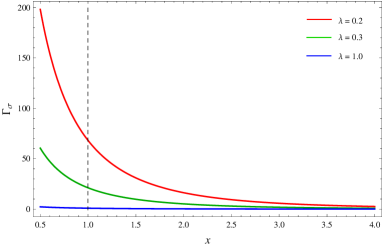
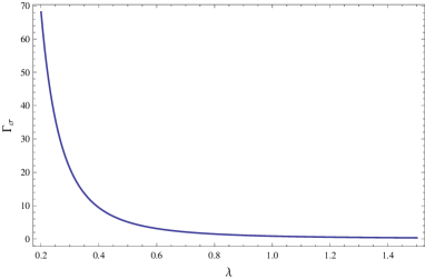
Figure 4: $\Gamma_{\sigma}$ as function of $x$ (left) and as function of $\lambda$ evaluated around the adiabatic sound horizon-crossing at $x\approx 1$ (right).

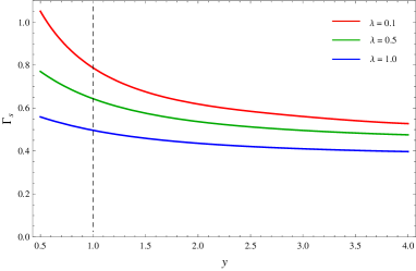
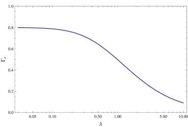
Figure 5: $\Gamma_{s}$ as function of $y$ (left) and as function of $\lambda$ evaluated around the entropy sound horizon-crossing at $y\approx 1$ (right).

Several comments are in order:

• The left figures in fig.4 and fig.5 show $\Gamma_{\sigma}$ or $\Gamma_{s}$ as functions of $x$ or $y$ respectively, for different values of $\lambda$. We take $\Gamma_{\sigma}$ as example. Since $x\equiv-c_{a}k\eta$, it implies that for mode with fixed $k$, when deep in the sound horizon ($x\gg 1$), corrections to the power spectrum from the cross-interactions are small. Again, this verifies previous argument that adiabatic and entropy perturbations can be treated as decoupled when they are deep inside the horizon, while when modes approach the horizon, i.e. $x\approx 1$, the modification to the power spectrum starts to increase [25]. The conclusion is the same for $\Gamma_{s}$.

• The most interesting point is that, as for the cross-correlation between adiabatic and entropy modes, the strength of the corrections to adiabatic/entropy spectra due to the presence of cross-couplings are also determined by the parameter $\lambda\equiv c_{e}/c_{a}$, i.e. the ratio of the sound speeds for entropy and adiabatic modes. It has been known that for $c_{a}=c_{e}$ i.e. $\lambda=1$, the cross-correlation and also the corrections to the “decoupled” spectra are proportional to the cross-coupling and thus are expected to be small [25, 26, 27]. However, from the right figures in fig.4 and fig.5, this corrections can be enhanced by small $\lambda$, that is for models with $c_{e}\ll c_{a}$. Especially, this enhancement is most significant for the adiabatic mode (fig.4). As explained before, when $c_{e}\ll c_{a}$ the entropy mode cross the horizon much earlier than the adiabatic mode, and thus act as a nearly constant (rather than highly oscillating) source on the evolution of adiabatic mode. Thus the smaller $\lambda$ is, the longer that the entropy mode behaves as a source, and the more significant this accumulative effect is.

• Inversely, this enhancement is not significant for the entropy mode. Actually from the right panel in fig.5, when $\lambda>1$ i.e. $c_{e}>c_{a}$, the correction to the power spectrum of entropy mode is suppressed when $\lambda$ goes large. Intuitively, this is because that, as is well-known, on super-horizon scales entropy modes can act as sources for the evolution of adiabatic mode, while inversely adiabatic mode can never act as a source for entropy modes. Thus, the larger $\lambda$ is, the earlier the adiabatic mode exits its horizon, and the less it affects the evolution of entropy modes. As an extremal case, one can verify that $\Gamma_{s}\rightarrow 0$ when $\lambda\rightarrow\infty$, which implies that in this case the entropy mode is not affected by adiabatic mode and evolves freely. Moreover from the right panel in fig.5, when $\lambda\rightarrow 0$, $\Gamma_{s}$ approaches a constant value rather than blowing up, since in this case the adiabatic mode which is highly oscillating affects the entropy mode with a nearly constant strength.

What we are eventually interested in are the spectra of the curvature and isocurvature perturbations, which are defined in (32) and (33). After using (34), the power spectrum for the curvature perturbation, including the leading-order corrections from the cross-interactions, and also including the corrections to both Green’s function and Hubble parameter in first-order slow-roll parameters, takes the form

$${}\mathcal{P}_{\mathcal{R}}(x) =\mathcal{P}^{(0)}_{\mathcal{R}}(x)+\mathcal{P}^{(2)}_{\mathcal{R}}(x)$$ (52)

$$\simeq\bar{\mathcal{P}}_{\mathcal{R}}\left(1+x^{2}\right)\left[1-2\epsilon-2s_{a}+\left(\nu_{\sigma}-\frac{3}{2}\right)f\left(\left(1+s_{a}\right)x\right)+s_{a}\frac{2x^{2}}{1+x^{2}}+\frac{\xi^{2}}{\left(1+x^{2}\right)}\Gamma_{\sigma}\left(x,\lambda\right)\right]\,,$$

where

$${}f(x)\equiv\frac{\pi x^{3}}{2\left(1+x^{2}\right)}\left(\frac{\partial}{\partial\nu}\left|H_{\nu}^{\left(1\right)}\left(x\right)\right|^{2}\right)_{\nu=\frac{3}{2}}\,.$$ (53)

In deriving the above expression, (80) and (80) are used. Similarly, the power spectrum for isocurvature perturbation is

$${}\mathcal{P}_{\mathcal{S}}(y)\simeq\bar{\mathcal{P}}_{\mathcal{S}}\left(1+y^{2}\right)\left[1-2\epsilon-2s_{e}+\left(\nu_{s}-\frac{3}{2}\right)f\left(\left(1+s_{e}\right)y\right)+s_{e}\frac{2y^{2}}{1+y^{2}}+\frac{\xi^{2}}{\left(1+y^{2}\right)}\Gamma_{s}\left(y,\lambda\right)\right]\,.$$ (54)

(42), (52) and (54) are the main results in this note, and can be viewed as generalizations of previous results, e.g. Eq.(78)-(80) in [27].

3.3.1 Deep Inside the Horizon

In [25], an oscillating mechanism was introduced to study the cross-correlations between perturbations, where it was found that when deep inside the Hubble horizon different modes evolve independently and can be considered as good mass eigenstates, thus the cross-correlations are indeed small. Intuitively, when deep inside the horizon, the system become weakly-coupled oscillators in Minkowski background in which the couplings among them are assumed to be small (of order slow-roll parameters). In fact, as an explicit confirmation, one can show that

$${}\Gamma_{c}(x,\lambda)\quad\xrightarrow[]{~{}~{}x\gg 1~{}~{}}\quad\frac{2+\lambda}{(1+\lambda)^{2}}\,,$$ (55)

which is independent of $x$. Similarly, it can be verified that $g_{\sigma,s}(x,\lambda)$ approach constant values (independent of $x$) when $x\gg 1$,

$$g_{\sigma}(x,\lambda)\rightarrow\frac{\lambda}{2\left(1+\lambda\right)}\,,\qquad g_{s}(y,\lambda)\rightarrow-\frac{\lambda}{2(1+\lambda)}\,,$$

thus

$${}\Gamma_{\sigma}(x,\lambda) \xrightarrow[]{~{}~{}x\gg 1~{}~{}}\quad-\frac{1}{2(1+\lambda)^{2}}\,,$$ (56)

$$\Gamma_{s}(y,\lambda) \xrightarrow[]{~{}~{}y\gg 1~{}~{}}\quad\frac{1+2\lambda}{2(1+\lambda)^{2}}\,.$$

From (55) and (56), it is obvious that

$$\max\Gamma_{i}\sim\mathcal{O}(1)\,,\qquad i=c,\sigma,s$$ (57)

thus we can conclude that when deep inside the horizon, the cross-correlation between curvature and isocurvature perturbation is always smaller than $\mathcal{O}(\xi)$, and the corrections to curvature/isocurvature perturbation due to this cross-interactions are always smaller than $\mathcal{O}(\xi^{2})$. This confirms previous investigation that the couplings between adiabatic/entropy perturbations can be neglected when modes are sub-Hubble.

However, as was firstly pointed out in [25] and was also analyzed in [26, 27], the most important lesson we get is that, the cross-interactions between adiabatic and entropy modes at linear level, which are negligible when modes are deep inside the horizons, are generated and amplified when modes cross their sound horizons. Our analysis in this work also confirms this fact.

3.3.2 Around Horizon-crossings

As has been stressed before, (42), (52) and (54) are the general expressions for power spectra for curvature and isocurvature perturbations and their cross power. Thus in general (42), (52) and (54) are needed to evaluate more precisely the amplitude of the powers and the spectral tilts around horizon crossing ($x_{\ast}\simeq 1+\epsilon_{a}$ and $y_{\ast}\simeq 1+\epsilon_{e}$). In this subsection, for our purpose to get a glance of the effects of the cross-correlations, we use superhorizon asymptotic limits of (42), (52) and (54) to evaluate various quantities around horizon-crossing.

The cross-power spectrum around adiabatic horizon-crossing is approximately

$${}\left.\mathcal{C}_{\mathcal{R}\mathcal{S}}\right|_{\frac{c_{a}k}{aH}=1}\simeq\left.\bar{\mathcal{P}}_{\mathcal{R}}\xi C(\lambda)\right|_{\frac{c_{a}k}{aH}=1}\,,\qquad\qquad\textrm{with}\;C(\lambda)\equiv\frac{1+\lambda-\ln(1+\lambda)-\gamma}{\lambda^{2}}\,,$$ (58)

where $\gamma\approx 0.5772$ is the Euler-Mascheroni constant. The spectral index is

$${}\left.n_{\mathcal{C}}\right|_{\frac{c_{a}k}{aH}=1} \equiv\left.\frac{\textrm{d}\ln\mathcal{C}_{\mathcal{R}\mathcal{S}}}{\textrm{d}\ln k}\right|_{\frac{c_{a}k}{aH}=1}\simeq\left.\left[-2\epsilon-\eta+\eta_{\xi}+\tilde{C}s_{a}-\left(\tilde{C}+1\right)s_{e}\right]\right|_{\frac{c_{a}k}{aH}=1}\,,$$ (59)

with $\tilde{C}\equiv 1-1/(\left(\lambda+1\right)C(\lambda))$. Note that in (58) and (59) all quantities are evaluated at the time of adiabatic sound horizon-crossing, i.e. $c_{a}k/aH=1$. From (58) it is explicit that up to first-order in the cross-interaction coupling $\xi$, the cross-power spectrum is $\sim C(\lambda)\xi$, it can be enhanced by small $\lambda$ due to the factor $C(\lambda)$, which scales as $1/\lambda^{2}$ for small $\lambda$. Note that for $\lambda=1$ i.e. for $c_{a}=c_{e}$, $C(\lambda)$ reduces to the familiar value $C(1)=2-\ln 2-\gamma\approx 0.7296$. Thus our calculations can be viewed as generalization of previous results in [26, 27].

Similarly, power spectra for the curvature and isocurvature perturbations around their respective horizon-crossings are

$${}\left.\mathcal{P}_{\mathcal{R}}\right|_{\frac{c_{a}k}{aH}=1} \simeq\left.\bar{\mathcal{P}}_{\mathcal{R}}\left(1-2\epsilon-2s_{a}\right)\left[1+\left(3-2\nu_{\sigma}\right)\left(\gamma-2+\ln 2\right)+\xi^{2}a_{\sigma}(\lambda)\right]\right|_{\frac{c_{a}k}{aH}=1}\,,$$ (60)

$$\left.\mathcal{P}_{\mathcal{S}}\right|_{\frac{c_{e}k}{aH}=1} \simeq\left.\bar{\mathcal{P}}_{\mathcal{S}}\left(1-2\epsilon-2s_{e}\right)\left[1+\left(3-2\nu_{e}\right)\left(\gamma-2+\ln 2\right)+\xi^{2}a_{s}(\lambda)\right]\right|_{\frac{c_{e}k}{aH}=1}\,,$$

where $a_{\sigma,s}(\lambda)$ are functions of $\lambda$ only. In getting (60), we have neglected all terms proportional to (such as) $\epsilon\xi^{2}$ etc., i.e. we only keep the leading-order contributions from $\xi^{2}$. For general $\lambda$, it is difficult to abstract analytical expressions for $a_{\sigma,s}(\lambda)$. Their numerical results are depicted in fig.6, Form which it is explicit that the corrections to both curvature and isocurvature power spectra can be enhanced by small $\lambda$.

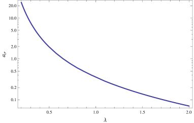
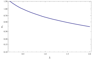
Figure 6: Numerical evaluation for $a_{\sigma}(\lambda)$ and $a_{s}(\lambda)$ as functions of $\lambda$.

In practice, it is convenient to introduce a dimensionless correlation angle $\Delta$ to characterize the strength of the cross-correlation:

$$\cos\Delta\equiv\frac{\mathcal{C}_{\mathcal{R}\mathcal{S}}}{\sqrt{\mathcal{P}_{\mathcal{R}}\mathcal{P}_{\mathcal{S}}}}\,.$$ (61)

From (42), (52) and (54), and using the fact that around the adiabatic sound horizon-crossing $\bar{\mathcal{P}}_{\mathcal{R}}/\bar{\mathcal{P}}_{\mathcal{S}}\approx\lambda$, we get the correlation angle around adiabatic sound horizon-crossing

$${}\left.\cos\Delta\right|_{\frac{c_{a}k}{aH}=1}\approx\left.\xi\sqrt{\lambda}\Gamma_{c}\left(x,\lambda\right)\right|_{\frac{c_{a}k}{aH}=1}\,.$$ (62)

In getting (62) we take the approximation under the assumption that the power spectra of curvature/isocurvature perturbations are still dominated by their “decoupled” values $\mathcal{P}_{\mathcal{R}}^{(0)}$ and $\mathcal{P}_{\mathcal{S}}^{(0)}$, i.e we assume that the corrections to the spectra would not exceed their respective decoupled values (they are indeed corrections). A more precise evaluation can be done by using (58) and (60) and the corresponding correlation angle around adiabatic horizon-crossing is depicted in fig.7.

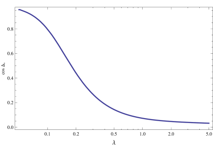
Figure 7: The correlation angle $\cos\Delta_{\ast}$ around adiabatic sound horizon-crossing as function of $\lambda$. Here $\xi$ is chosen as 0.1

It immediately follows that, for $\lambda=1$ (the case for canonical kinetic terms or multi-DBI case with $c_{a}=c_{e}=c_{s}$) or larger (a concrete example is the case for multi-field $k$-inflation [22, 40], where $c_{a}=c_{s}\ll 1$ and $c_{e}=1$), the correlation angle is small and the cross-correlation between curvature and isocurvature perturbations are suppressed. However, as has been stressed before, for models with $c_{e}<c_{a}$ or even $c_{e}\ll c_{a}$, the cross-correlations will be highly enhanced by small $\lambda$. Thus, for models with $\xi$ much larger than the slow-roll parameters which are of order $10^{-2}$ or with $c_{e}\ll c_{a}$, the curvature and isocurvature perturbations are highly correlated when exiting the adiabatic sound horizon. In this case, the “decoupled” power spectra $\mathcal{P}_{\mathcal{R}}^{(0)}$ and $\mathcal{P}_{\mathcal{S}}^{(0)}$ are not good approximations, and the cross-correlations between curvature and isocurvature perturbations much be taken into account.

4 Conclusion and Discussion

In this paper we investigate the effects of cross-interactions between curvature perturbation and isocurvature perturbations on cross-power spectrum and the power spectra of curvature/isocurvature perturbations themselves, before and around horizon crossing. Previous investigations of the cross-correlations are based on diagonalizting the coupled equations of motion [25, 26, 27]. However, one can verify that, for models with different adiabatic/entropy speeds of sound, the “diagonalization” cannot be done easily and thus the treatments in [25, 26, 27] cannot be viewed as good approximation in this case. Thus, in this work, the cross-couplings are taken as two-point interaction vertices, and a field-theoretical perturbative approach is taken to evaluate the cross-power spectrum etc.

The main results in this work are summarized in (42), (52) and (54). Our analysis confirms previous conclusion that the cross-correlations, which can be safely neglected when modes are deep inside the horizons, are generated when modes cross their sound horizons [25]. Moreover, the most interesting phenomenon get in this work is that the cross-correlation (and also the corrections to power spectra of curvature/isocurvature perturbations) can be enhanced by small $c_{e}/c_{a}$ ratio, where $c_{a}$ and $c_{e}$ are the sound speeds of curvature and isocurvature perturbations respectively. As has been stressed before, this happens since in models with $c_{e}/c_{a}\ll 1$, in the process curvature perturbation getting closed to the adiabatic horizon, the isocurvature perturbation is already well outside its entropic horizon and behaves as a nearly constant (rather than highly oscillating) background, which acts as a nearly constant source on the curvature perturbation. This fact causes the amplifications of both cross-spectrum between curvature and isocurvature modes and also the corrections to the spectra of curvature and isocurvature perturbations.

To end this note, we would like to comment some limitations and also possible extensions of the investigation in this note:

• The approach in evaluating the cross-correlation and the corrections to (decoupled) power spectra of curvature and isocurvature perturbation is perturbative. The coupling $\xi$ is assumed to be small. This is indeed the case for canonical kinetic terms, but in models (e.g.) considered in this note, $\xi$ may be not small enough for the perturbative approach to be valid.

• In general the cross-couplings between adiabatic and entropy modes are complicated. In this note we make the assumption that the cross-coupling $\xi$ in (24) is slow-varying in time. This is a simplification for abstracting the basic properties of the cross-correlations, but definitely a more detailed analysis of the cross-interactions is needed.

• Moreover, in this note we only focus on the cross-correlations around the horizon-crossing. In order to get the resulting primordial power spectra on large scales, and to compare the predictions of a multi-inflation model with observations, one must then solve the coupled system described by the full equations of motion. In some particular case and within the slow-roll approximation, one can arrive at an analytical expression for the spectra on large scales, e.g. through the “transfer matrix” method [5]. In general, however, a numerical approach is needed.

• As has been stressed before, (42), (52) and (54) are the general expressions for power spectra for curvature and isocurvature perturbations and their cross power. In general, in multi-field models it may not be permitted to use the later time (superhorizon limit) asymptotic expressions to evaluate the powers around horizon-crossing, since there may be inflation scenarios where the perturbation evolve quickly after horizon crossing and never reach the asymptotic values. Thus in general (42), (52) and (54) are needed to evaluate more precisely the amplitude of the powers and also the spectral indices around horizon-crossings ($\frac{c_{a}k}{aH}=1$ and $\frac{c_{e}k}{aH}=1$ respectively).

• One possible application of the formalism and result in this work is that, as firstly pointed out in [30], one should expect the “transfer” of non-Gaussianities from entropy perturbations to the adiabatic perturbation (see fig.8), if the cross-correlations between adiabatic mode and entropy modes are larger than $\sim\mathcal{O}(\epsilon)$ and thus cannot be neglected. Especially, there are inflation scenarios in which the non-linearities in adiabatic mode itself are small, however the possible large non-Gaussianities in entropy modes could transfer to the non-Gaussianities in adiabatic mode through the cross-interactions.

  

  

  Figure 8: Diagrammatic representations of exchanging non-Gaussianities from entropy mode to non-Gaussianities of adiabatic mode.

  This would bring new features to non-Gaussianities such as new shapes of momenta configurations [30, 61].

Appendix A “In-in” Formalism

The “in-in formalism” (also dubbed as “Schwinger-Keldysh formalism”, or “Closed-time path formalism”) [45, 46, 47] (see also [48, 49] for a nice review) is a perturbative approach for solving the evolution of expectation values over a finite time interval. It is therefore ideally suited not only to backgrounds which do not admit an S-matrix description, such as inflationary backgrounds.

In the calculation of S-matrix in particle physics, the goal is to determine the amplitude for a state in the far past $|\psi\rangle$ to become some state $|\psi^{\prime}\rangle$ in the far future,

$$\langle\psi^{\prime}|S|\psi\rangle=\langle\psi^{\prime}(+\infty)|\psi(-\infty)\rangle\,.$$

Here, conditions are imposed on the fields at both very early and very late times. This can be done because that in Minkowski spacetime, states are assumed to be non-interacting at far past and at far future, and thus are usually taken to be the free vacuum, i.e., the vacuum of the free Hamiltonian $H_{0}$. The free vacuum are assumed to be in “one-to-one” correspondence with the true vacuum of the whole interacting theory, as we adiabatically turn on and turn off the interactions between $t=-\infty$ and $t=+\infty$.

While the physical situation we are considering here is quite different. Instead of specifying the asymptotic conditions both in the far past and far future, we develop a given state forward in time from a specified initial time, which can be chosen as the beginning of inflation. In the cosmological context, the initial state is usually chosen as free vacuum, such as Bunch-Davis vacuum, since at very early times when perturbation modes are deep inside the Hubble horizon, according to the equivalence principle, the interaction-picture fields should have the same form as in Minkowski spacetime.

The Hamiltonian can be split into a free part and an interacting part: $H=H_{0}+H_{\textrm{i}}$. The time-evolution operator in the interacting picture is well-known

$${}U(\eta_{2},\eta_{1})=\mathrm{T}\exp\left(-i\int_{\eta_{1}}^{\eta_{2}}dt^{\prime}H_{\textrm{i}\textrm{I}}(\eta^{\prime})\right)\,,$$ (63)

where subscript “I” denotes interaction-picture quantities, T is the time-ordering operator. Our present goal is to relate the interacting vacuum at arbitrary time $|\Omega_{\textrm{I}}(t)\rangle$ to the free vacuum $|0_{\textrm{I}}\rangle$ (e.g., Bunch-Davis vacuum). The trick is standard. First we may expand $|\Omega_{\textrm{I}}(\eta)\rangle$ in terms of eigenstates of free Hamiltonian $H_{0}$, $|\Omega_{\textrm{I}}(\eta)\rangle=\sum_{n}|n_{\textrm{I}}\rangle\,\langle n_{\textrm{I}}|\Omega_{\textrm{I}}(\eta)\rangle$, then we evolve $|\Omega_{\textrm{I}}(\eta)\rangle$ by using (63)

$${}|\Omega_{\textrm{I}}(\eta_{2})\rangle=U(\eta_{2},\eta_{1})|\Omega_{\textrm{I}}(\eta_{1})\rangle=|0_{\textrm{I}}\rangle\,\langle 0_{\textrm{I}}|\Omega_{\textrm{I}}\rangle+\sum_{n\geq 1}e^{+iE_{n}(\eta_{2}-\eta_{1})}\,|n_{\textrm{I}}\rangle\,\langle n_{\textrm{I}}|\Omega_{\textrm{I}}(\eta_{1})\rangle\,.$$ (64)

From (64), we immediately see that, if we choose $\eta_{2}=-\infty(1-i\epsilon)$, all excited states in (64) are suppressed. Thus we relate interacting vacuum at $\eta=-\infty(1-i\epsilon)$ to the free vacuum $|0\rangle$ as

$$|\Omega_{\textrm{I}}(-\infty(1-i\epsilon))\rangle=|0_{\textrm{I}}\rangle\,\langle 0_{\textrm{I}}|\Omega_{\textrm{I}}\rangle$$ (65)

Thus, the interacting vacuum at arbitrary time $\eta$ is given by

$$|\textrm{VAC},\textrm{in}\rangle \equiv|\Omega_{\textrm{I}}(\eta)\rangle=U(\eta,-\infty(1-i\epsilon))|\Omega_{\textrm{I}}(-\infty(1-i\epsilon))\rangle$$ (66)

$$=\mathrm{T}\exp\left(-i\int^{\eta}_{-\infty(1-i\epsilon)}d\eta^{\prime}\,H_{\textrm{i}\textrm{I}}(\eta^{\prime})\right)|0_{\textrm{I}}\rangle\,\langle 0_{\textrm{I}}|\Omega_{\textrm{I}}\rangle\,.$$

The expectation value of operator $\hat{\mathcal{O}}(\eta)$ at arbitrary time $\eta$ is evaluated as

$${}\langle\hat{\mathcal{O}}(\eta)\rangle \equiv\frac{\langle\textrm{VAC},\textrm{in}|\hat{\mathcal{O}}(\eta)|\textrm{VAC},\textrm{in}\rangle}{\langle\textrm{VAC},\textrm{in}|\textrm{VAC},\textrm{in}\rangle}$$ (67)

$$=\left\langle 0_{\textrm{I}}\left|\bar{\mathrm{T}}\exp\left(i\int^{\eta}_{-\infty{(1+i\epsilon)}}d\eta^{\prime}H_{1\textrm{I}}(\eta^{\prime})\right)\,\hat{\mathcal{O}}_{\textrm{I}}(\eta)\,\mathrm{T}\exp\left(-i\int^{\eta}_{-\infty{(1-i\epsilon)}}d\eta^{\prime}H_{\textrm{i}\textrm{I}}(\eta^{\prime})\right)\right|0_{\textrm{I}}\right\rangle\,,$$

where $\bar{\textrm{T}}$ is the anti-time-ordering operator.

For simplicity, we denote

$$-\infty(1-i\epsilon)\equiv-\infty^{+}\,,\qquad\qquad-\infty(1+i\epsilon)\equiv-\infty^{-}\,,$$ (68)

since, e.g., $-\infty^{+}$ has a positive imaginary part. Now let us focus on the time-order in (67). In standard S-matrix calculations, operators between $\langle 0|$ and $|0\rangle$ are automatically time-ordered. While in (67), from right to left, time starts from infinite past, or $-\infty^{+}$ precisely, to some arbitrary time $\eta$ when the expectation value is evaluated, then back to $-\infty^{-}$ again. This time-contour forms a closed-time path, so “in-in” formalism is sometimes called “closed-time path” (CTP) formalism.

The starting point of perturbation theory is the free theory two-point correlation functions. In canonical quantization procedure, we write a scalar field as

$$\phi_{\bm{k}}(\eta)=u(k,\eta)a_{\bm{k}}+u^{\ast}(k,\eta)a^{{\dagger}}_{-\bm{k}}\,,$$ (69)

where $u(k,\eta)$ is the mode function for $\phi_{\bm{k}}(\eta)$ (in practice, $u_{k}(\eta)$ and $u^{\ast}_{k}(\eta)$ are two linear-independent solutions of equation of motion for $\phi_{\bm{k}}(\eta)$, which are Wroskian normalized and satisfy some initial or asymptotic conditions ).

The free two-point function takes the form

$${}\left\langle 0\left|\phi_{\bm{k}_{1}}(\eta_{1})\phi_{\bm{k}_{2}}(\eta_{2})\right|0\right\rangle\equiv(2\pi)^{3}\delta^{3}(\bm{k}_{1}+\bm{k}_{2})G_{k_{1}}(\eta_{1},\eta_{2})\,,$$ (70)

with

$${}G_{k_{1}}(\eta_{1},\eta_{2})\equiv u_{k_{1}}(\eta_{1})u^{\ast}_{k_{1}}(\eta_{2})\,.$$ (71)

In this work, we take (70) and (71) as the starting point.

Now Taylor expansion of (67) gives

• 0th-order

  $${}\left\langle\hat{\mathcal{O}}(\eta)\right\rangle^{(0)}=\langle 0_{\textrm{I}}|\hat{\mathcal{O}}_{\textrm{I}}(\eta)|0_{\textrm{I}}\rangle\,.$$ (72)

• 1st-order (one interaction vertex)

  $${}\left\langle\hat{\mathcal{O}}(\eta)\right\rangle^{(1)}=2\,\textrm{Re}\left[-i\,\int^{\eta}_{{-\infty^{+}}}d\eta^{\prime}\,\left\langle 0_{\textrm{I}}\left|\hat{\mathcal{O}}_{\textrm{I}}(\eta)\,H_{\textrm{i}\textrm{I}}(\eta^{\prime})\right|0_{\textrm{I}}\right\rangle\right]\,.$$ (73)

• 2nd-order (two interaction vertices)

  $$\left\langle\hat{\mathcal{O}}(\eta)\right\rangle^{(2)} =-2\,\textrm{Re}\left[\int^{\eta}_{{-\infty^{+}}}d\eta^{\prime}\,\int^{\eta^{\prime}}_{{-\infty^{+}}}d\eta^{\prime\prime}\,\left\langle 0_{\textrm{I}}\left|\hat{\mathcal{O}}_{\textrm{I}}(\eta)\,H_{\textrm{i}\textrm{I}}(\eta^{\prime})\,H_{\textrm{i}\textrm{I}}(\eta^{\prime\prime})\right|0_{\textrm{I}}\right\rangle\right]$$ (74)

  $$\qquad\qquad+\int^{\eta}_{{-\infty^{-}}}d\eta^{\prime}\int^{\eta}_{{-\infty^{+}}}d\eta^{\prime\prime}\,\left\langle 0_{\textrm{I}}\left|H_{\textrm{i}\textrm{I}}(\eta^{\prime})\,\hat{\mathcal{O}}_{\textrm{I}}(\eta)\,H_{\textrm{i}\textrm{I}}(\eta^{\prime\prime})\right|0_{\textrm{I}}\right\rangle\,.$$

Appendix B Mathematics

In this work, we frequently account exponential/sine/cosine-integral functions, their definitions are

$$\text{Ei}(z) =-\int_{-z}^{\infty}\frac{e^{-t}}{t}\,dt$$ (75)

$$\text{Si}(z) =\int_{0}^{z}\frac{\sin(t)}{t}dt\,,\qquad\qquad\text{Ci}(z)=-\int_{z}^{\infty}\frac{\cos(t)}{t}\,dt\,.$$

In evaluating various integrals, the following properties are frequently used:

• For $x>0$,

  $$\textrm{Ei}\left(-ix\right)=\text{Ci}(x)-i\left(\text{Si}(x)+\frac{\pi}{2}\right)\,,$$

  where $\textrm{Ci}(x)$ and $\textrm{Si}(x)$ take real values.

• $\textrm{Ei}(-i\infty)=-i\pi$, $\textrm{Ei}(+i\infty)=i\pi$, $\textrm{Ci}(+\infty)=0$, $\textrm{Ci}(-\infty)=i\pi$ and $\textrm{Si}(\pm\infty)=\pm\frac{\pi}{2}$.

• When $x\rightarrow+\infty$

  $$\textrm{Ei}(-ix)+i\pi=\frac{e^{-ix}}{x}\left(i-\frac{1}{x}+\mathcal{O}(x^{-2})\right)\,.$$ (76)

Appendix C Comparison with Previous Results with $c_{a}=c_{e}$

In order to compare calculations in this note to previous results, we consider a special case $c_{a}=c_{e}$, or $\lambda=1$. Our goal is to show that the field-theoretical perturbative approach taken in this note is essentially equivalent to previous “diagonalization” method taken in [25, 26, 27]. We take $\Gamma_{c}$ as example.

It is straightforward calculations to verify that

$${}\Gamma_{c}(x_{\ast},1) =\frac{1}{2}\left(x_{\ast}^{2}-1\right)\left[2\text{Ci}(2x_{\ast})\cos(2x_{\ast})-(\pi-2\text{Si}(2x_{\ast}))\sin(2x_{\ast})\right]$$ (77)

$$\qquad-x\left[2\text{Ci}(2x_{\ast})\sin(2x_{\ast})+(\pi-2\text{Si}(2x_{\ast}))\cos(2x_{\ast})\right]+2$$

$$\equiv\frac{\pi}{2}x_{\ast}^{3}\left(J_{\frac{3}{2}}\left(x_{\ast}\right)\left.\frac{\partial J_{\nu}\left(x_{\ast}\right)}{\partial\nu}\right|_{\nu=\frac{3}{2}}+Y_{\frac{3}{2}}\left(x_{\ast}\right)\left.\frac{\partial Y_{\nu}\left(x_{\ast}\right)}{\partial\nu}\right|_{\nu=\frac{3}{2}}\right)$$

$$=\frac{\pi}{4}x_{\ast}^{3}\left(\frac{\partial}{\partial\nu}\left|H_{\nu}^{\left(1\right)}\left(x_{\ast}\right)\right|^{2}\right)_{\nu=\frac{3}{2}}\,.$$

Recall that the dimensionless power spectrum for a scalar field in dS background takes the form

$$\mathcal{P}(\eta,k)=\bar{\mathcal{P}}F_{\nu}\left(x\right)\,,$$ (78)

where $\bar{\mathcal{P}}\equiv\left(\frac{H_{\ast}}{2\pi}\right)^{2}\frac{1}{c_{s}}$ is the asymptotic super-Hubble limit (i.e. $x_{\ast}\rightarrow 0$) of the spectrum and $x\equiv-c_{s}k\eta$ and

$${}F_{\nu}\left(x\right) \equiv\frac{\pi}{2}x^{3}\left|H_{\nu}^{\left(1\right)}\left(x\right)\right|^{2}$$ (79)

$$=\frac{\pi}{2}x^{3}\left|H_{\frac{3}{2}}^{\left(1\right)}\left(x\right)\right|^{2}+\left(\nu-\frac{3}{2}\right)\frac{\pi}{2}x^{3}\left(\frac{\partial}{\partial\nu}\left|H_{\nu}^{\left(1\right)}\left(x\right)\right|^{2}\right)_{\nu=\frac{3}{2}}+\cdots$$

$$\equiv 1+x^{2}+\left(\nu-\frac{3}{2}\right)f(x)+\cdots\,,$$

with

$${}f(x)\equiv\frac{\pi x^{3}}{2\left(1+x^{2}\right)}\left(\frac{\partial}{\partial\nu}\left|H_{\nu}^{\left(1\right)}\left(x\right)\right|^{2}\right)_{\nu=\frac{3}{2}}\,.$$ (80)

Thus in this case the factor $\Gamma_{c}(x_{\ast},\lambda)$ which is get from theoretical perturbative calculations is nothing but the coefficient of the term which is first-order in $\nu-\frac{3}{2}$ in the expansion of the exact power spectrum:

$$\Gamma_{c}(x_{\ast},1)=\frac{1}{2}f(x_{\ast})\,.$$ (81)

Thus (77) can be compared with (e.g.) Eq.(79) in [27]. This result is as expected, since in this case the original coupled equations can be diagonalized, and two approaches (i.e. “calculating the correlator perturbatively” and “expanding the exact correlator perturbatively”) are essentially equivalent.

Appendix D Mode Solutions

We take the adiabatic equation of motion in (27) as example. It is convenient to introduce new variable $x\equiv-c_{a}k\eta$ to characterize the time-evolution. After straightforward algebras and keeping terms up to first-order in slow-varying parameters, the equation becomes:

$${}\frac{d^{2}u_{\sigma}}{dx^{2}}-\frac{s_{a}}{x}\frac{du_{\sigma}}{dx}+\left(1+2s_{a}-\frac{1}{x^{2}}\left(2+3\epsilon+\frac{3}{2}\eta_{\epsilon}+s_{a}\right)\right)u_{\sigma}=0\,,$$ (82)

where various slow-varying parameters are defined in (20). Its solution which corresponds to the traditional BD vacuum is

$${}u_{\sigma}=Cx^{\frac{1}{2}\left(1+s_{a}\right)}H_{\nu_{\sigma}}^{\left(1\right)}\left(\left(1+s_{a}\right)x\right)\,,$$ (83)

where $C$ is the normalization constant to be determined and $\nu_{\sigma}=\frac{3}{2}+\frac{1}{2}\left(2\epsilon+\eta_{\epsilon}+s_{a}\right)$.

On the other hand, when modes are deep inside the horizon i.e. $x\ll 1$, the above equation becomes

$$\frac{d^{2}u_{\sigma}}{dx^{2}}-\frac{s_{a}}{x}\frac{du_{\sigma}}{dx}+\left(1+2s_{a}\right)u_{\sigma}=0\,,$$ (84)

and its solution which satisfies the Wronskian normalization is

$$u_{\sigma}\equiv\left(\bar{H}\left(1-\epsilon\right)\right)^{\frac{s_{a}}{2}}\frac{e^{i\left(1+s_{a}\right)x}}{\sqrt{2(\bar{c}_{s}k)^{1+s_{a}}}}\,x^{\frac{s_{a}}{2}}\,,$$ (85)

where we use a “$\bar{\phantom{A}}$” to denote constant values for the slow-varying quantities, e.g. $H\sim\bar{H}a^{-\epsilon}$ etc. Using the fact that for $x\gg 1$, the solution (83) has the following asymptotic expression:

$$u_{\sigma}\rightarrow Cx^{\frac{1}{2}s}e^{i(1+s)x}\sqrt{\frac{2}{\pi}}\frac{e^{-i\frac{\pi}{4}}e^{-\frac{1}{2}i\pi\nu}}{\sqrt{1+s}}\,,$$ (86)

the constant in (83) can be determined as

$$C=\frac{\sqrt{\pi}}{2}\bar{H}^{\frac{s_{a}}{2}}\left(\bar{c}_{s}k\right)^{-\frac{1+s_{a}}{2}}\left(1+\frac{s_{a}}{2}\right)e^{\frac{i\pi}{2}\left(\nu_{\sigma}+\frac{1}{2}\right)}\,.$$ (87)

This gives the solution in (28). It is similar for the entropy mode solution in (28).

References

- [1] E. Komatsu et al. [WMAP Collaboration], Astrophys. J. Suppl. 180, 330 (2009)
- [2] D. H. Lyth and A. Riotto, Phys. Rept. 314, 1 (1999) [arXiv:hep-ph/9807278].
- [3] D. Langlois, Phys. Rev. D 59, 123512 (1999) [arXiv:astro-ph/9906080].
- [4] L. Amendola, C. Gordon, D. Wands and M. Sasaki, Phys. Rev. Lett. 88, 211302 (2002) [arXiv:astro-ph/0107089].
- [5] D. Wands, N. Bartolo, S. Matarrese and A. Riotto, Phys. Rev. D 66, 043520 (2002) [arXiv:astro-ph/0205253].
- [6] L. A. Kofman and A. D. Linde, Nucl. Phys. B 282, 555 (1987).
- [7] V. F. Mukhanov and M. I. Zelnikov, Phys. Lett. B 263, 169 (1991).
- [8] D. Polarski and A. A. Starobinsky, Nucl. Phys. B 385, 623 (1992).
- [9] D. Wands and J. Garcia-Bellido, Helv. Phys. Acta 69, 211 (1996) [arXiv:astro-ph/9608042].
- [10] J. Garcia-Bellido and D. Wands, Phys. Rev. D 54, 7181 (1996) [arXiv:astro-ph/9606047].
- [11] V. F. Mukhanov and P. J. Steinhardt, Phys. Lett. B 422, 52 (1998) [arXiv:astro-ph/9710038].
- [12] A. A. Starobinsky, S. Tsujikawa and J. Yokoyama, Nucl. Phys. B 610, 383 (2001) [arXiv:astro-ph/0107555].
- [13] B. J. W. van Tent, Class. Quant. Grav. 21, 349 (2004) [arXiv:astro-ph/0307048].
- [14] A. A. Starobinsky and J. Yokoyama, arXiv:gr-qc/9502002.
- [15] C. Gordon, D. Wands, B. A. Bassett and R. Maartens, Phys. Rev. D 63, 023506 (2001) [arXiv:astro-ph/0009131].
- [16] D. Langlois and F. Vernizzi, JCAP 0702, 017 (2007) [arXiv:astro-ph/0610064].
- [17] D. Langlois and F. Vernizzi, Phys. Rev. Lett. 95, 091303 (2005) [arXiv:astro-ph/0503416].
- [18] D. Langlois and F. Vernizzi, Phys. Rev. D 72, 103501 (2005) [arXiv:astro-ph/0509078].
- [19] F. Di Marco, F. Finelli and R. Brandenberger, Phys. Rev. D 67, 063512 (2003) [arXiv:astro-ph/0211276].
- [20] F. Di Marco and F. Finelli, Phys. Rev. D 71, 123502 (2005) [arXiv:astro-ph/0505198].
- [21] B. A. Bassett, S. Tsujikawa and D. Wands, Rev. Mod. Phys. 78, 537 (2006) [arXiv:astro-ph/0507632].
- [22] D. Langlois and S. Renaux-Petel, JCAP 0804, 017 (2008) [arXiv:0801.1085 [hep-th]].
- [23] D. A. Easson, R. Gregory, D. F. Mota, G. Tasinato and I. Zavala, JCAP 0802, 010 (2008) [arXiv:0709.2666 [hep-th]].
- [24] M. x. Huang, G. Shiu and B. Underwood, Phys. Rev. D 77, 023511 (2008) [arXiv:0709.3299 [hep-th]].
- [25] N. Bartolo, S. Matarrese and A. Riotto, Phys. Rev. D 64, 083514 (2001) [arXiv:astro-ph/0106022].
- [26] C. T. Byrnes and D. Wands, Phys. Rev. D 74, 043529 (2006) [arXiv:astro-ph/0605679].
- [27] Z. Lalak, D. Langlois, S. Pokorski and K. Turzynski, JCAP 0707, 014 (2007) [arXiv:0704.0212 [hep-th]].
- [28] S. Tsujikawa, D. Parkinson and B. A. Bassett, Phys. Rev. D 67, 083516 (2003) [arXiv:astro-ph/0210322].
- [29] K. Y. Choi, L. M. H. Hall and C. van de Bruck, JCAP 0702, 029 (2007) [arXiv:astro-ph/0701247].
- [30] N. Bartolo, S. Matarrese and A. Riotto, Phys. Rev. D 65, 103505 (2002) [arXiv:hep-ph/0112261].
- [31] D. Langlois, S. Renaux-Petel, D. A. Steer and T. Tanaka, Phys. Rev. Lett. 101, 061301 (2008) [arXiv:0804.3139 [hep-th]].
- [32] D. Langlois, S. Renaux-Petel, D. A. Steer and T. Tanaka, Phys. Rev. D 78, 063523 (2008) [arXiv:0806.0336 [hep-th]].
- [33] D. Langlois, S. Renaux-Petel and D. A. Steer, arXiv:0902.2941 [hep-th].
- [34] S. Renaux-Petel and G. Tasinato, JCAP 0901, 012 (2009) [arXiv:0810.2405 [hep-th]].
- [35] F. Arroja, S. Mizuno and K. Koyama, JCAP 0808, 015 (2008) [arXiv:0806.0619 [astro-ph]].
- [36] E. Kawakami, M. Kawasaki, K. Nakayama and F. Takahashi, arXiv:0905.1552 [astro-ph.CO].
- [37] S. Mizuno, F. Arroja, K. Koyama and T. Tanaka, Phys. Rev. D 80, 023530 (2009) [arXiv:0905.4557 [hep-th]].
- [38] J. L. Lehners and S. Renaux-Petel, arXiv:0906.0530 [hep-th].
- [39] C. T. Byrnes and G. Tasinato, JCAP 0908, 016 (2009) [arXiv:0906.0767 [astro-ph.CO]].
- [40] Xian Gao, JCAP 0806, 029 (2008) [arXiv:0804.1055 [astro-ph]].
- [41] Xian Gao and Bin Hu, arXiv:0903.1920 [astro-ph.CO].
- [42] X. Gao, M. Li and C. Lin, arXiv:0906.1345 [astro-ph.CO].
- [43] S. Renaux-Petel, arXiv:0907.2476 [hep-th].
- [44] S. Mizuno, F. Arroja and K. Koyama, arXiv:0907.2439 [hep-th].
- [45] J. S. Schwinger, J. Math. Phys. 2 (1961) 407.
- [46] E. Calzetta and B. L. Hu, Phys. Rev. D 35, 495 (1987).
- [47] R. D. Jordan, Phys. Rev. D 33, 444 (1986).
- [48] S. Weinberg, Phys. Rev. D 72, 043514 (2005) [arXiv:hep-th/0506236].
- [49] S. Weinberg, Phys. Rev. D 74, 023508 (2006) [arXiv:hep-th/0605244].
- [50] S. H. Tye, J. Xu and Y. Zhang, arXiv:0812.1944 [hep-th].
- [51] X. Ji and T. Wang, arXiv:0903.0379 [hep-th].
- [52] M. Li, C. Lin, T. Wang and Y. Wang, arXiv:0805.1299 [astro-ph].
- [53] W. Xue and B. Chen, arXiv:0806.4109 [hep-th].
- [54] S. W. Li and W. Xue, arXiv:0804.0574 [astro-ph].
- [55] Q. G. Huang, arXiv:0903.1542 [hep-th].
- [56] Q. G. Huang, JCAP 0906, 035 (2009) [arXiv:0904.2649 [hep-th]].
- [57] Y. F. Cai and W. Xue, arXiv:0809.4134 [hep-th].
- [58] Y. F. Cai and H. Y. Xia, Phys. Lett. B 677, 226 (2009) [arXiv:0904.0062 [hep-th]].
- [59] X. Gao and F. Xu, JCAP 0907, 042 (2009) [arXiv:0905.0405 [hep-th]].
- [60] X. Chen, M. x. Huang, S. Kachru and G. Shiu, JCAP 0701, 002 (2007) [arXiv:hep-th/0605045].
- [61] X. Chen and Y. Wang, arXiv:0911.3380 [hep-th].