SU(2) lattice gauge theory in 2+1 dimensions:
critical couplings from twisted boundary conditions and universality

Abstract

We present a precision determination of the critical coupling $\beta_{c}$ for the deconfinement transition in pure SU(2) gauge theory in $2+1$ dimensions. This is possible from universality, by intersecting the center vortex free energy as a function of the lattice coupling $\beta$ with the exactly known value of the interface free energy in the 2D Ising model at criticality. Results for lattices with different numbers of sites $N_{t}$ along the Euclidean time direction are used to determine how $\beta$ varies with temperature for a given $N_{t}$ around the deconfinement transition.

1 Introduction

It is widely accepted today that the deconfinement transition in pure SU($N$) gauge theories at finite temperature is driven by the dynamics of center vortices [1]. In the vortex picture of confinement, Wilson loops acquire a disordering phase factor from every vortex that they link with. The area law for timelike Wilson loops in the pure gauge theory comes from the percolation of spacelike vortex sheets in the confined phase. Their free energies have been measured over the deconfinement phase transition at finite temperature in the $3+1$ dimensional pure SU(2) gauge theory from ratios of partition functions with ’t Hooft’s twisted boundary conditions in temporal planes, forcing odd numbers of $Z_{2}$ center vortices through those planes, over the periodic ensemble with even numbers [2, 3]. A Kramers-Wannier duality is then observed by comparing the behaviour of these center vortices with that of ’t Hooft’s electric fluxes which yield the free energies of static charges in a well-defined (UV-regular) way [4], with boundary conditions to mimic the presence of ’mirror’ (anti)charges in neighbouring volumes. This duality follows that between the Wilson loops of the 3-dimensional $Z_{2}$-gauge theory and the 3D-Ising spins, reflecting the universality of the center symmetry breaking transition. Here we study the vortex free energies of pure SU(2) in $2+1$ dimensions over the deconfinement transition because the relevant interface free energies of its universal partner, the self-dual Ising model in 2 dimensions, are all known analytically. Moreover, the vortex free energies in $2+1$ dimensions are much cheaper to simulate and discretisation effects vanish more rapidly than in $3+1$ dimensions. Together these reasons allow for numerical studies of much higher precision.

In Sections 2 and 3 we briefly outline the basic concepts and our numerical procedure. Our results are presented in Sec. 4. These include the precise determination of the critical coupling for various lattices with up to $N_{t}=9$ sites in the Euclidean time direction, an analysis of the finite volume corrections and a brief comparison with the corrections to scaling in the 2D Ising model. We then determine how the critical coupling depends on $N_{t}$, including $1/N_{t}$ corrections, and use this result to derive how the lattice coupling $\beta$ varies with temperature for a given fixed $N_{t}$ around the deconfinement transition. This is needed, for example, for a detailed finite-size scaling analysis of the vortex free energies in 2+1 dimensional SU(2) [5].

2 Concepts and Methods

For pure SU(2) gauge theory, ’t Hooft’s twisted boundary conditions fix the total number of $Z_{2}$ vortices modulo 2 through each plane of a finite box [6]. Twist in a plane corresponds to an ensemble with an odd number of $Z_{2}$ vortices through that plane.

In a $L^{2}\times 1/T$ Euclidean box, we can distinguish between two types of twist. Magnetic twist is defined in the purely spatial plane and forces vortices that run along the temporal direction. They may spread independently of the temperature $T$ and play no role in the deconfinement transition: their free energy is expected to vanish in the thermodynamic limit at all temperatures which has been demonstrated explicitly in $3+1$ dimensions [7]. On the other hand, vortices from twist in the two temporal planes are squeezed more and more as $T$ is increased. They may no longer spread arbitrarily and this is what drives the phase transition.

In this paper we’re interested in configurations with a twist in one of the temporal planes. If we denote the partition function of this ensemble by $Z_{tw}(L,T)$, its free energy per $T$ is defined via the ratio

$$Z_{tw}(L,T)/Z_{0}(L,T)=e^{-F_{tw}(L,T)}$$ (1)

where $Z_{0}$ is the partition function of the periodic ensemble.

As we approach the thermodynamic limit, $Z_{tw}/Z_{0}$ converges to a non-trivial fixed point at the critical temperature. It can therefore be used as a phenomenological coupling in the same manner as the Binder cumulant. Typically, one uses the pairwise intersections of Binder cumulant curves from different lattice sizes to estimate the critical coupling or temperature [8, 9]. Using a ratio of partition functions in this way was proposed by Hasenbusch for the 3D Ising model [10].

Here we can go a step further. Since SU(2) in 2+1 dimensions is in the same universality class as the 2D Ising model, the the value of $Z_{tw}/Z_{0}$ at the fixed point is exactly known. A single temporal twist in SU(2) corresponds to a single anti-periodic direction on a $N\times N$ Ising lattice. This forces an odd number of spin interfaces perpendicular to the anti periodic direction. The corresponding ratio of partition functions $Z_{ap}/Z_{pp}$ in the Ising model gives the free energy of the system in the same way as equation (1). In both cases, configurations of minimum action/energy dominate the partition function. Thus, in the thermodynamic limit, the free energy of a single spacelike vortex in SU(2) is identified with the free energy of a single interface in the 2D square Ising model at the respective critical points. This universal value is given by [11]

$$\lim_{N\rightarrow\infty}Z_{ap}(T_{c})/Z_{pp}(T_{c})=1/(1+2^{3/4}).$$ (2)

Figure 1: Universality

For SU(2) on the lattice, $1/T=N_{t}a$ where $N_{t}$ is the number of sites in the time direction and the lattice spacing $a\equiv a(\beta)$ depends on the coupling. So the critical temperature $T_{c}$ corresponds to a critical lattice coupling $\beta_{c,\infty}$ for each $N_{t}$. The subscript $\infty$ reminds us that we only have a strict phase transition and hence critical coupling in the limit of infinite spatial volume. Still, the intersection of $Z_{tw}/Z_{0}$ with the universal value (2) gives a reliable estimate of $\beta_{c,\infty}(N_{t})$ provided that the spatial length $L=N_{s}a$ is large enough. This will be more precise in general than the estimates obtained via pairwise intersections.

We assume a finite size scaling (FSS) behaviour of the form

$$Z_{tw}/Z_{0}=1/(1+2^{3/4})+b(\beta-\beta_{c})N_{s}^{1/\nu}+cN_{s}^{-\omega}+\dots\;,$$ (3)

where $\omega$ is a correction to scaling exponent that should be approximately independent of $N_{t}$, and $\nu=1$ is exactly known from the 2D Ising model. Furthermore, $\beta_{c}\equiv\beta_{c,\infty}(N_{t})$, and we define a ’pseudo-critical coupling’ in a finite volume, $\beta_{c}(N_{t},N_{s})$, by the requirement that the corrections to the universal value in (3) vanish. These estimates then converge to the infinite volume critical coupling $\beta_{c,\infty}(N_{t})$ as

$$\beta_{c}(N_{t},N_{s}) = \beta_{c,\infty}(N_{t})-d(N_{t})\,N_{s}^{-(\omega+1/\nu)}+\dots$$ (4)

Here, the coeffiecient $d=c/b$ is an $N_{t}$ dependent fit parameter.

For notational simplicity we will hereafter drop the subscript $\infty$ on the critical coupling. Unless $N_{s}$ is explicitly mentioned, $\beta_{c}$ refers to the infinite volume limit. We have used a variety of spatial lattice sizes and the above scaling formula (3) to first find $\beta_{c}(N_{t},N_{s})$ for $N_{t}=4,\,5,\,6,\,7,\,8$ and $9$ with high precision, in order to then determine the corresponding $\beta_{c}(N_{t})$ from fitting the volume dependence of $\beta_{c}(N_{t},N_{s})$ by (4).

Figure 2: Fitted curves for $N_{t}=5$, selected for clarity.

3 Numerical recipe

Twist was implemented in the usual way [13]. We kept periodic boundary conditions but flipped the coupling $\beta\rightarrow-\beta$ of a stack of plaquettes perpendicular to the plane of the twist. In other words, we introduced a $Z_{2}$ Dirac string that is closed by lattice periodicity. The result is a transformation of the usual Wilson action.

In practice, the overlap of $Z_{tw}$ and $Z_{0}$ is poor. To overcome this we interpolated in the number of flipped plaquettes using the snake algorithm of Ref. [14]. This was combined with the other variance reduction tricks therein.

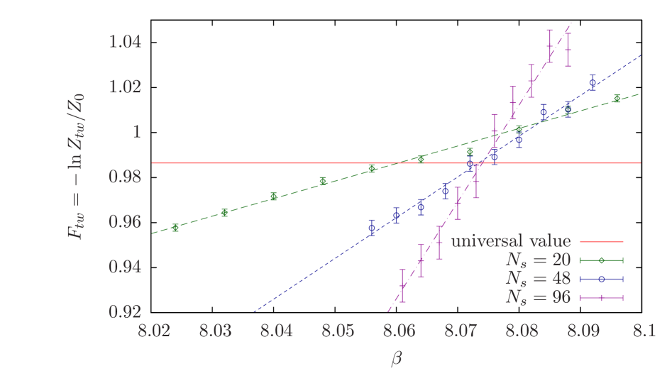
For each combination of $N_{t}$ and $N_{s}$ we performed simulations for $\sim 10$ values of $\beta$ around the intersection of $Z_{tw}/Z_{0}$ with the exact Ising value (2). Random errors were estimated via the boostrap method. Since SU(2) lattice gauge theory is less computationally expensive in 2+1 dimensions than in 3+1 dimensions, we were able to perform a very large number of measurements. $1-30$ million configurations were used for each $\beta$, depending on the lattice size.

It turns out that the free energy $F_{tw}(\beta)=-\ln Z_{tw}/Z_{0}$ has less curvature than $Z_{tw}/Z_{0}$ near the critical point, so it’s a better candidate for linear approximation. Therefore we performed least squares fits, with parameters $f_{1}$ and $\beta_{c}$, of the form

$$F_{tw}(\beta)=f_{1}\,(\beta-\beta_{c})+\ln(1+2^{3/4})$$ (5)

to obtain estimates $\beta_{c}=\beta_{c}(N_{t},N_{s})$ for the critical lattice coupling. In each case the reduced $\chi^{2}$ was $\sim 1$, which justifies the linear ansatz (5). See Fig. 2 for some representative fits.

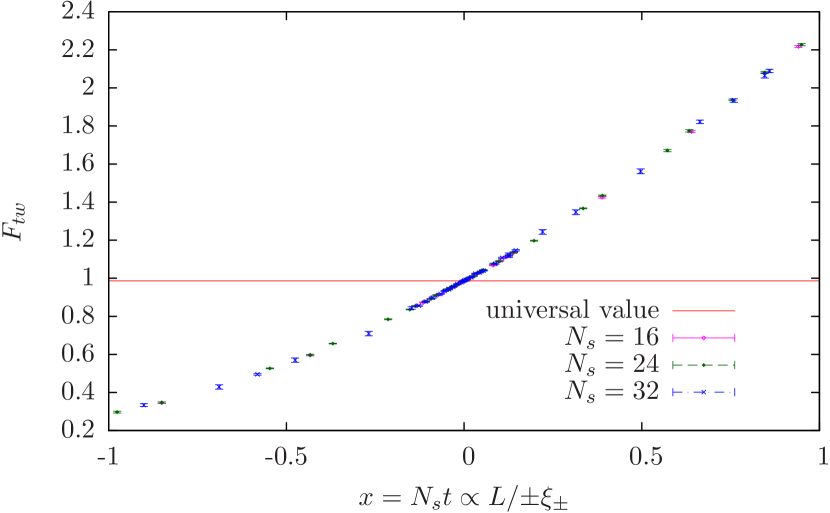
Note, however, that a small reduced $\chi^{2}$ does not exclude the existence of significant systematic errors in $\beta_{c}(N_{t},N_{s})$. On finite lattices, $F_{tw}(\beta)$ has positive curvature near the critical coupling, so $\beta_{c}$ tends to be underestimated. To control this, we carefully chose the size of our fitting windows. For each $N_{t}$, we performed precise measurements of $F_{tw}$ in a quadratic fitting window for one or more of our smallest lattices. By writing $F_{tw}$ as a function of the finite size scaling variable

$$x=N_{s}\,t\propto\pm L/{\xi_{\pm}}\,,$$ (6)

where $t=T/T_{c}-1$ is the reduced temperature and $\xi=\xi_{\pm}^{0}|t|^{-\nu}$ are the correlation lengths for $T\mathrel{\hbox to0.0pt{\lower 1.5pt\hbox{\small\hskip 1.0pt$<$}\hss}\hskip 1.0pt\raise 3.0pt\hbox{\small$>$}}T_{c}$ with $\nu=1$ for the 2D Ising model, we were able to translate this data to larger $N_{s}$. See Fig. 3 for an example of FSS data collapse in a large window for several lattice sizes. The relationship between temperature and coupling is described in Section 4.4. It requires a paramerisation of $\beta_{c}$ vs $N_{t}=1/T_{c}a_{c}$, which we roughly obtained using literature values of the critical coupling and our own preliminary results. The translated data was used to estimate the slope and curvature of $F_{tw}(\beta)$ near the critical point for large lattices without performing additional simulations. We then adjusted the linear fitting windows such that the systematic errors in $\beta_{c}(N_{t},N_{s})$ should be less than one quarter of the quoted random error for each extrapolated $\beta_{c}(N_{t}).$

Figure 3: FSS data collapse for $16^{2}\times 4$, $24^{2}\times 4$ and $32^{2}\times 4$.

4 Results

4.1 Determining $\beta_{c}(N_{t})$

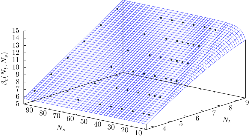
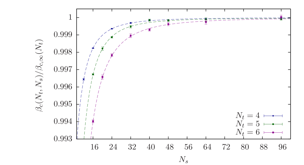
We have obtained estimates of $\beta_{c}(N_{t})$ for every $N_{t}$ between 4 and 9. In each case we used 8 spatial lattice sizes, keeping an aspect ratio of approximately 3:1 for the smallest lattice and using a maximum lattice size of $96^{2}\times N_{t}$. See Fig. 5 for plots of $\beta_{c}(N_{t},N_{s})$ vs $N_{s}$ for $N_{t}=4$, 5 and 6. The data was fitted according to the equation (4) with all three parameters free. The plots for $N_{t}=$ 7, 8 and 9 look very similar. Note the rapid convergence to the infinite volume values, which Hasenbusch also observed for the pairwise intersection of $Z_{ap}/Z_{pp}$ curves in the 3D Ising model [10]. He found much more rapid convergence than for the intersections of Binder cumulants.

Figure 4: All values for $\beta_{c}(N_{t},N_{s})$ obtained in this work. The error bars are generally smaller than the symbols, and the surface was rendered from the fits to (4) with $d(N_{t})=0.134\,N_{t}^{\omega+2}-0.51\,N_{t}^{\omega}$ according to (8) with $d_{1}=0$.

Figure 5: Critical beta estimates vs $N_{s}$ relative to their infinite volume limits for $N_{t}=4,\,5$ and $6$, and the corresponding fits to (4).

$N_{t}$	$N_{s}$ used	$\beta_{c}(N_{t},64)$	$\beta_{c}(N_{t},96)$	$\beta_{c,\infty}(N_{t})$	$\omega$ (fit)	$\chi^{2}$/dof.	$\beta_{c,\infty}(N_{t})\big{|}_{\omega=1.61}$	$\chi^{2}$/dof.	Lit. values
4	12, 16, 24, 32, 40, 48, 64, 96	6.53611(19)	6.53648(37)	6.53661(13)	1.47(6)	0.98	6.53640(10)	1.62	6.483(26)$\dagger$ 6.52(3)$\ddagger$ 6.588(25)$\S$
5	16, 20, 24, 32, 40, 48, 64, 96	8.07392(74)	8.07402(39)	8.07463(38)	1.73(15)	1.35	8.07488(26)	1.29	8.143(57)$\dagger$
6	16, 20, 24, 32, 40, 48, 64, 96	9.6002(12)	9.6029(11)	9.60265(49)	1.48(7)	0.37	9.60185(33)	0.60	9.55(4)$\ddagger$
7	20, 24, 28, 32, 40, 48, 64, 96	11.1164(15)	11.1181(36)	11.1194(29)	1.38(43)	1.74554	11.1181(13)	1.54	–
8	24, 28, 32, 36, 40, 48, 64, 96	12.6301(32)	12.6342(53)	12.6348(40)	1.66(52)	0.89	12.6348(19)	0.89	–
9	24, 28, 32, 40, 48, 56, 64, 96	14.1488(94)	14.131(11)	14.1418(68)	1.96(79)	0.60	14.1446(39)	0.52	–

Table 1: Summary of results from the $N_{s}^{2}\times N_{t}$ lattices specified in columns 1 and 2 with the critical couplings for the largest two $N_{s}$ given explicitly in columns 3 and 4; the infinite volume extrapolations from fits to Eq. (4) are shown in column 5 with the resulting exponents $\omega$ and $\chi^{2}$/dof. in columns 6 and 7. Columns 8 and 9 show the same extrapolations when using the global average $\omega=1.61(9)$ in all fits. Literature values are quoted for comparison from Refs. ^† [16], ^‡ [17] and ^§ [18].

We summarize our results in Table 1. For each $N_{t}$ we include the estimates $\beta_{c}(N_{t},N_{s})$ from our two largest lattices as well as the fitted values of $\beta_{c}(N_{t})$. It’s clear from the reduced $\chi^{2}$s that the data is very well described by the FSS ansatz (4).

For $N_{t}=$ 4, 5 and 6 we were able to surpass the precision of current literature values of the critical couplings by two orders of magnitude. These lattices also gave us good precision for the correction to scaling exponent $\omega$. Our results for $N_{t}=$ 7, 8, 9 are somewhat less precise, especially the fitted values for $\omega$. This is because the lattices used had smaller aspect ratios and we collected fewer statistics. Still, $\omega$ is consistent between each of the fits. In all, we obtain a weighted average for $\omega$ of 1.61(9), which is also consistent with the value of 1.64 obtained by Engels et al. [15] in early study of Polyakov loop averages.

For reference, we have included extrapolations of the critical coupling with $\omega$ fixed at 1.61. Due to correlations, the quoted errors for $\beta_{c}(N_{t})|_{\omega=1.61}$ should be taken with a grain of salt. Nevertheless, fixing $\omega$ may lead to more accurate values of $\beta_{c}(N_{t})$ for our large $N_{t}$ results.

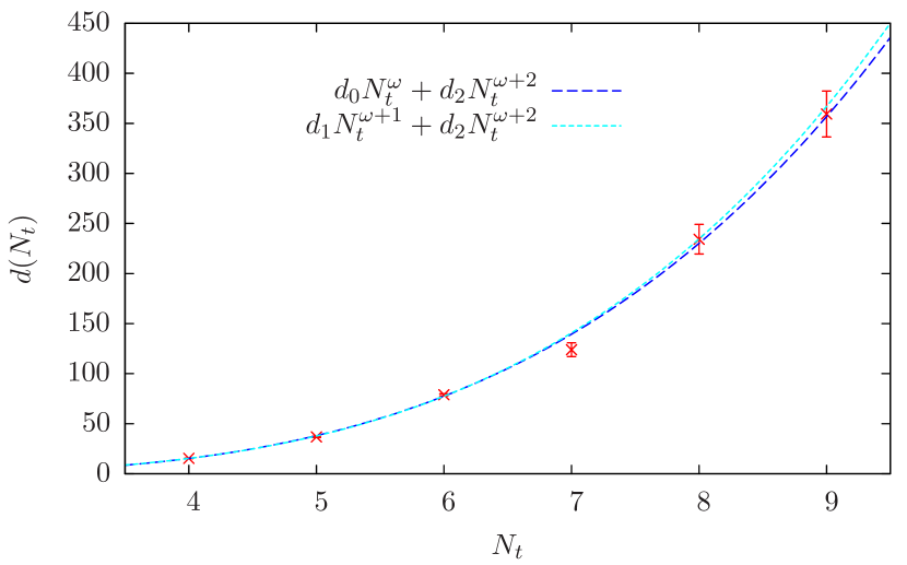
We furthermore obtain the fit parameter $d(N_{t})$ in (4) for each of the six $N_{t}$ values. This in turn allows us to fit its $N_{t}$ dependence. Using a two parameter form $d_{\mathrm{fit}}(N_{t})=d_{\gamma}\,N_{t}^{\gamma_{\mathrm{fit}}}$ with a single effective exponent $\gamma_{\mathrm{fit}}$, a fairly good description is obtained with $\gamma_{\mathrm{fit}}=3.97(7)$ (and $d_{\gamma}=0.06(1)$). This fit works best for the smaller $N_{t}$ but it deteriorates somewhat towards $N_{t}=9$. The $N_{t}$ dependence of $d(N_{t})$ might well be determined by several competing terms with nearby exponents and is thus difficult to extract reliably from the data. Alternatively, using 3 parameter fits of the form

$$d_{\mathrm{fit}}(N_{t})=d_{\delta}\,N_{t}^{\delta}+d_{\gamma}\,N_{t}^{\gamma_{\mathrm{fit}}}\,,$$ (7)

we obtain $\gamma_{\mathrm{fit}}=3.8(2)$ for $\delta=0$, $\gamma_{\mathrm{fit}}=3.7(4)$ for $\delta=\omega$, or $\gamma_{\mathrm{fit}}=3.5(6)$ for $\delta=\omega+1$, for example, where we have used $\omega=1.61$ corresponding to our global fit for the correction to scaling exponent $\omega$. Because $\omega+2=3.61$, this suggests that one might also try a form

$$d_{\mathrm{fit}}(N_{t})=d_{0}\,N_{t}^{\omega}+d_{1}\,N_{t}^{\omega+1}+d_{2}\,N_{t}^{\omega+2}\,,$$ (8)

with $\omega$ fixed at 1.61. This form is particularly interesting because it will allow us below to parametrise the finite-size corrections entirely in terms of the aspect ratio in the form $N_{t}/N_{s}$. Unfortunately, the coefficients $d_{0}$ and $d_{1}$ of the two subleading powers in $\omega$ are much too correlated to determine all the 3 parameters in this fit reliably from the available data. But we can get good fits with either $d_{1}=0$ or $d_{0}=0$, see Fig. 6. Keeping the resulting two parameters fixed afterwards, a further fit to the remaining one ($d_{1}$ or $d_{0}$) then reproduces a zero result with very high accuracy (i.e., values smaller than $10^{-4}$ in either case).

  

Figure 6: The parameter $d(N_{t})$ from the fits of $\beta_{c}(N_{t},N_{s})$ to Eq. (4) together with 2 parameter fits of its $N_{t}$ dependence via the form in Eq. (8) with $d_{1}=0$ (long-dashed) and $d_{0}=0$ (short-dashed), respectively.

It’s interesting to check how much was gained by using the exact universal value (2) instead of pairwise intersections. To this end we performed the pairwise intersection method for $N_{t}=4$. See Table 2 for the results. The left side of the table shows the intersection coupling for lattices with $N_{s}$ and $N_{s}^{{}^{\prime}}=N_{s}/2$. On the right hand side are comparative results from intersections with the universal Ising reference line.

It follows from Eq. (3) that the pairwise intersection points should scale like Eq. (4), except with $-d\rightarrow 2(2^{\omega}-1)d$. As such, we’ve included an extrapolation with $\omega=1.61$ fixed.

Since the simulations were not catered for pairwise intersections, it may be unfair to directly compare the extrapolations in Table 2. Still, due to the rapid convergence of $\beta_{c}(N_{t},N_{s})$, our data was quite well centered around the intersection points except for the smallest lattices. And knowing what value of $Z_{tw}/Z_{0}$ to concentrate the efforts around was a big advantage of our method. Anticipating the location of pairwise intersection points is much more troublesome. In all, it’s clear that the exploitation of the universal number $F_{tw}(\beta_{c})=\ln(1+2^{3/4})$ gave a significant boost to the precision of our results.

$N_{s}^{{}^{\prime}}-N_{s}$	intersection coupling	$N_{s}$	$\beta_{c}(4,N_{s})$ from (5)
12-24	6.5539(19)	24	6.53240(14)
16-32	6.5451(12)	32	6.53459(23)
24-48	6.53816(37)	48	6.53569(16)
32-64	6.53706(45)	64	6.53611(19)
48-96	6.53756(94)	96	6.53648(37)
Extrap.	6.53558(45)		6.53640(10)∗
$\chi^{2}$/dof.	1.45		1.62

Table 2: Comparison of critical couplings obtained for $N_{t}\!=\!4$ via pairwise intersection (left) and via intersection with the universal reference line (right). ^∗This is the extrapolation with all 8 available $N_{s}$ values included, as quoted in the $8^{\mathrm{th}}$ column of Table 1. The restriction to the 5 values of $N_{s}\in(24,96)$ listed here gives 6.53641(5), which is consistent but has an unnaturally small error.

4.2 2D Ising model

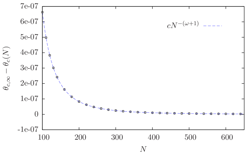
For the sake of comparison we repeated our procedure for the square 2D Ising model. Taking the exact solutions for $Z_{ap}$ and $Z_{pp}$ on $N\times N$ lattices from Ref. [19], we used Mathematica [20] to find $\theta=k_{B}T/J$ at the intersection of $Z_{ap}/Z_{pp}$ with the universal value (2). Here $J$ is the coupling of nearest neighbour spins. In Figure 7 we plot the results for $N\in[100,640]$. The error bars are representative only (the errors are limited only by the working precision and should be smaller than $10^{-16}$).

Again we fit the data with a FSS ansatz of the form

$$\theta_{c}(N)=\theta_{c,\infty}-cN^{-(\omega+1)}.$$ (9)

In this case, we hold $\theta_{c,\infty}$ fixed at the known value of $2/\ln(1+\sqrt{2})$. We obtain for the correction to scaling exponent $\omega=2+\delta$ with $\delta\to 0^{+}$ as we increase the lower bound $N_{\mathrm{min}}$ used in the fit, i.e., $\omega$ tends towards 2 from above ($\delta$ starts at around $2\cdot 10^{-4}$ for the full range of $N$ shown in Fig. 7, and it falls below $10^{-5}$ at $N_{\mathrm{min}}$ around 400). Since the exponent of the leading irrelevant operator that breaks rotational invariance is predicted to be exactly 2 [21], our result is consistent with the conjecture of Ref. [22] that the only irrelevant operators that appear in the 2D nearest neighbour Ising model are those due to the lattice breaking of rotational symmetry. This may be tested on a triangular 2D lattice where the leading irrelevant operator to break rotational invariance leads to $\omega=4$ instead, while the leading rotationally invariant operator would give an isotropic correction to scaling with $\omega=2$ in either case [22].

On the other hand, our correction exponent for SU(2) is clearly at odds with $\omega=2$. In this case, it’s possible that there exists an irrelevant operator that is not present in the 2D Ising model or the corresponding conformal theory. It may be more likely, however, that our exponent is really an effective exponent. When there are several nearby competing exponents it is extremely difficult to extract the smallest one from simulations.

Figure 7: Critical coupling estimate vs $N$ for the 2D Ising model together with a fit by (9) yielding $\omega=2.0002$ for $N_{\mathrm{min}}=100$, or $\omega=2.00001$ for $N_{\mathrm{min}}=400$.

4.3 $\beta_{c}$ vs $N_{t}$

Figure 8: $\beta_{c}(N_{t})$ vs $N_{t}$. Note the deviation from linearity.

In 2+1 dimensions the coupling $g_{3}^{2}$ has the dimension of mass and sets the scale for the theory. The bare lattice coupling is then given by [17]

$$\beta=\frac{2N_{c}}{ag_{3B}^{2}}\,,\quad g_{3B}^{2}=g_{3}^{2}+c_{1}ag_{3}^{4}+c_{2}a^{2}g_{3}^{6}+\dots$$ (10)

Substituting this expansion into $\beta$ gives

$$\frac{\beta}{2N_{c}}=\frac{1}{ag_{3}^{2}}-c_{1}-c_{2}ag_{3}^{2}+\dots\,.$$ (11)

Note now that $T=1/(N_{t}a)$. So at criticality we have

$$\frac{\beta_{c}(N_{t})}{2N_{c}}=\frac{T_{c}}{g_{3}^{2}}\,N_{t}-c_{1}-c_{2}\,\frac{g_{3}^{2}}{T_{c}}\,\frac{1}{N_{t}}+\dots$$ (12)

The first correction to the bare lattice coupling gives the y-intercept of $\beta_{c}(N_{t})$ vs $N_{t}$ while the second is a correction to linearity for small $N_{t}$.

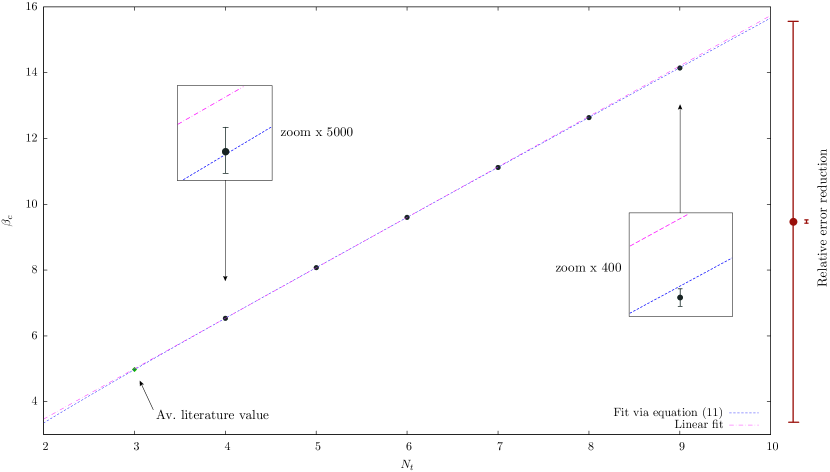
In Fig. 8 we plot our results for $\beta_{c}(N_{t})$, using the fitted values with $\omega$ free. We include also the estimate $\beta_{c}(3)=4.978(35)$, which is the average of the literature values 4.943(13) [16] and 5.013(15) [18]. For the uncertainty we use their standard error, which is simply half their difference. The actual error used here has very little influence on the results. The data is fitted with both a straight line and with a function of the form (12). To the naked eye, it would appear that the linear approximation is good all the way down to $N_{t}=3$. However, our data is precise enough to pick up the deviation from linearity. In fact, the reduced $\chi^{2}$ of the linear fit is $\sim 70$. With, the $1/N_{t}$ correction the reduced $\chi^{2}$ drops to 1.5. Thus, the data is very well described by Eq. (12). We obtain the parameterisation

$$\beta_{c}(N_{t})=1.5028(21)\,N_{t}+0.705(21)-0.718(49)\,\frac{1}{N_{t}}\,.$$ (13)

Consequently, from Eq. (12) for $N_{c}=2$, we obtain

$$T_{c}\,=\,0.3757(5)\;g_{3}^{2}\,.$$ (14)

This is compatible with the estimate $T_{c}/g_{3}^{2}\simeq 0.385$ with an error of $\pm 0.010$ as quoted in Ref. [18]. Note that it is the $1/N_{t}$ corrections included in (12) that lead to a somewhat lower value here as compared to [18] which is however within their estimate of the systematic uncertainties. In order to translate our estimate into units of the zero-temperature string tension $\sigma$ we use the mean value with standard error of the four $N=2$ values for $\sqrt{\sigma}/g_{3}^{2}$ listed in [26] as pairs of upper and lower bounds including some systematic uncertainty, which gives $\sqrt{\sigma}/g_{3}^{2}=0.3347(5)$. With uncorrelated error propagation, this together with our estimate (15) then corresponds to

$$T_{c}/\sqrt{\sigma}\,=\,1.1225(23)\,,$$ (15)

which agrees very well with the corresponding result of [16], $T_{c}/\sqrt{\sigma}\,=\,1.1224(90)$.

From Eq. (13), the other constants in Eq. (12) are analogously determined as

$$c_{1}\,=\,-0.176(5)\,,\;\;c_{2}=0.0675(5)\,.$$ (16)

Eq. (13) can be used to obtain accurate estimates of the critical coupling at large values of $N_{t}$. We can furthermore include the finite-size corrections in our ’pseudo-critical coupling’ (4) for the intersection, at finite $N_{s}$, of the vortex free energy $F_{tw}$ in (5) with the universal value $\ln(1+2^{3/4})$. If we assume a form as given in Eq. (8), these corrections can be expressed entirely in terms of the aspect ratio $A\equiv N_{t}/N_{s}$. In particular, the leading corrections for small $A$ can then conveniently be combined with the large $N_{t}$ expansion (12) as follows,

$$\beta_{c}(N_{t},N_{s}) = \Big{(}4\,\frac{T_{c}}{g_{3}^{2}}-d_{2}\,A^{\rho}\Big{)}\,N_{t}-4c_{1}-d_{1}\,A^{\rho}$$

$$\hskip 5.69046pt-\Big{(}4c_{2}\,\frac{g_{3}^{2}}{T_{c}}+d_{0}\,A^{\rho}\Big{)}\,\frac{1}{N_{t}}+\dots\,,$$

where we again used $N_{c}=2$ and $\rho=\omega+1/\nu$. Since $\nu=1$ in the 2D Ising model, our global fit to the correction to scaling exponent $\omega$ amounts to $\rho=\omega\!+\!1=2.61(9)$. If we assume $d_{1}=0$, our fits yield

$$d_{2}=0.134(4)\,,\;\;d_{0}=-0.51(9)\;,$$ (18)

and a reduced $\chi^{2}$ of 2.7. With $d_{0}=0$ on the other hand,

$$d_{2}=0.155(7)\,,\;\;d_{1}=-0.21(4)\;,$$ (19)

and a reduced $\chi^{2}$ of 2.6. The corresponding fits are shown in Fig. 6. Apart from this systematic uncertainty in the otherwise elegant parametrisation (8) of the finite-size corrections, we have therefore determined all parameters in (4.3).

4.4 $\beta$ vs temperature

So far, we have studied the critical couplings for different $N_{t}$. These were measured from the intersection of the vortex free energy with the universal value. Since $T=1/N_{t}a$, and with the temperature kept fixed at $T_{c}$, this means that the corresponding lattice spacing at criticality scales inversely with $N_{t}$, i.e., for two lattices with $N_{t}$ and $N_{t}^{\prime}$ we have $a_{c}^{\prime}/a_{c}=N_{t}/N_{t}^{\prime}$, and at the given order in $1/N_{t}$ (in the infinite volume limit),

$$\frac{\beta_{c}(N_{t}^{\prime})}{4}-\frac{\beta_{c}(N_{t})}{4}=\frac{T_{c}}{g_{3}^{2}}\,(N_{t}^{\prime}-N_{t})-c_{2}\frac{g_{3}^{2}}{T_{c}}\Big{(}\frac{1}{N_{t}^{\prime}}-\frac{1}{N_{t}}\Big{)}+\dots\,.$$ (20)

Alternatively, we can consider a change of $N_{t}$ as a change in temperature at a fixed lattice spacing. In particular, a simulation done at criticality of the $N_{t}^{\prime}$ lattice, with $a_{c}(N_{t}^{\prime})=a(N_{t})$, then corresponds to a simulation at $T=(N_{t}^{\prime}/N_{t})T_{c}$ on the $N_{t}$ lattice, i.e., with $\beta\equiv\beta(a)$, we have

$$\beta_{c}(N_{t}^{\prime})=\beta(1/(N_{t}^{\prime}T_{c}))=\beta(1/(N_{t}T))\,.$$ (21)

Denoting this coupling by $\beta(T,N_{t})$, we can therefore use Eq. (20) to write down an equation for the temperature dependence of the lattice coupling near criticality at a fixed $N_{t}$,

$$\frac{\beta(T,N_{t})}{4}-\frac{\beta_{c}(N_{t})}{4}=\frac{N_{t}}{g_{3}^{2}}\,\big{(}T-T_{c}\big{)}-c_{2}\frac{g_{3}^{2}}{N_{t}}\Big{(}\frac{1}{T}-\frac{1}{T_{c}}\Big{)}+\dots\,.$$ (22)

If we compare simulations at different $N_{t}$ but with the same aspect ratio $A=N_{t}/N_{s}$ in a finite volume, we can furthermore include the finite-size corrections here as in (4.3). In terms of the reduced temperature $t=T/T_{c}-1$, we then have

$$\beta(T,N_{t},N_{s}) =\beta_{c}(N_{t},N_{s})+C(N_{t},N_{s})\,t+\dots\,,$$ (23)

$$C(N_{t},N_{s}) =\Big{(}4\,\frac{T_{c}}{g_{3}^{2}}-d_{2}\,A^{\rho}\Big{)}\,N_{t}+\Big{(}4c_{2}\,\frac{g_{3}^{2}}{T_{c}}+d_{0}\,A^{\rho}\Big{)}\,\frac{1}{N_{t}}\,,$$

where $\beta_{c}(N_{t},N_{s})$ is the pseudo-critical coupling in Eq. (4.3), and $\beta(T,N_{t},N_{s})$ refers to the temperature dependence of the coupling near this $\beta_{c}$ at fixed $N_{t}$ and $N_{s}$. The terms neglected are either subleading in the aspect ratio $A$, or of order $1/N_{t}^{2}$, or they are of higher order in the reduced temperature. Note that criticality in a finite volume is a fuzzy concept, of course. As before, it is here defined by $\beta=\beta_{c}$ at $t=0$ from the intersection of the vortex free energy with the universal value, c.f., Eq. (5).

Note that the linear relationship between lattice coupling $\beta$ and temperature in Eq. (23), which is of the form

$$T/T_{c}=1+(\beta-\beta_{c})/C\,,$$ (24)

can be used to control the temperature at fixed $N_{t}$ and $N_{s}$ by adjusting the lattice coupling. The corresponding procedure for SU(2) in 3+1 dimensions, where $\beta$ depends logarithmically on temperature, was used in [2]. We will exploit this to perform a detailed finite-size scaling analysis of the vortex free energy $F_{tw}$ in 2+1 dimensional SU(2) with high precision in a future paper. This will include scaling of data from various $N_{t}$ lattices.

5 Summary

We have shown that very accurate determinations of the critical couplings for the SU(2) deconfinement transition in 2+1 dimensions are possible from intersecting vortex free energies with the known universal value from the 2D square Ising model at criticality. This allowed us to determine the critical coupling for lattices with up to $N_{t}=9$ sites in the Euclidean time direction. Its $N_{t}$ dependence could be determined with an accuracy sufficient to require significant $1/N_{t}$ corrections to the linear behaviour of the continuum limit. As a result, the slope of this behaviour given by $T_{c}/g_{3}^{2}$ might have been somewhat overestimated in the past. In particular, we observe that rather large $N_{t}$ may be required to reach the asymptotic continuum behaviour, even though it should be approached much more rapidly here than in 3+1 dimensions.

References

- [1] J. Greensite, Prog. Part. Nucl. Phys. 51 (2003) 1.
- [2] Ph. de Forcrand and L. von Smekal, Phys. Rev. D 66 (2002) 011504(R).
- [3] L. von Smekal and Ph. de Forcrand, in Confinement, Topology and other Non-Perturbative Aspects of QCD, J. Greensite and S. Olejnik (eds.), NATO Science Series, Kluwer (2002) 287.
- [4] Ph. de Forcrand and L. von Smekal, Nucl. Phys. Proc. Suppl. 106 (2002) 619.
- [5] S. Edwards and L. von Smekal, in preparation.
- [6] G. ’t Hooft, Nucl. Phys. B 153 (1979) 141.
- [7] L. von Smekal and Ph. de Forcrand, Nucl. Phys. Proc. Suppl.} 119 (2003) 655.
- [8] K. Binder, Z. Phys. B 43 (1981) 119.
- [9] K. Binder and E. Luijten, Phys. Rept. 344 (2001) 179.
- [10] M. Hasenbusch, Monte Carlo simulation with fluctuating boundary conditions, CERN-TH-6826-93 (1993).
- [11] H. Park and M. den Nijs, Phys. Rev. B 38 (1988) 565.
- [12] M. Caselle and M. Hasenbusch, Nucl. Phys. B 470 (1996) 435.
- [13] K. Kajantie, L. Karkkainen and K. Rummukainen, Nucl. Phys. B 357 (1991) 693.
- [14] Ph. de Forcrand, M. D’Elia and M. Pepe, Phys. Rev. Lett. 86 (2001) 1438.
- [15] J. Engels, E. Kehl, H. Satz and B. Waltl, Phys. Rev. Lett. 55 (1985) 2839.
- [16] J. Liddle and M. Teper, arXiv:0803.2128.
- [17] J. Engels, et al., Nucl. Phys. Proc. Suppl. 53 (1997) 420.
- [18] M. Teper, Phys. Lett. B 313 (1993) 417.
- [19] M.-C. Wu, M.-C. Huang, Y.-P. Luo and T.-M. Liaw, J. Phys. A: Math. Gen. 32 (1999) 4897.
- [20] Mathematica, Version 7.0, Wolfram Research, Inc., Champaign, IL, 2008.
- [21] M. Campostrini, A. Pelissetto, P. Rossi and E. Vicari, Phys. Rev. E 57 (1998) 184.
- [22] M. Caselle, M. Hasenbusch, A. Pelissetto and E. Vicari, J. Phys. A 35 (2002) 4861.
- [23] J. C. Le Guillou and J. Zinn-Justin, J. Phys. Lett. 46 (1985) L137.
- [24] M. Barma and M. E. Fisher, Phys. Rev. B 31 (1985) 5954.
- [25] P. Calabrese, M. Caselle, A. Celi, A. Pelissetto and E. Vicari, J. Phys. A 33 (2000) 8155.
- [26] B. Bringoltz and M. Teper, Phys. Lett. B 645 (2007) 383.