The large-scale environment of low surface brightness galaxies

Abstract

Context. The exact formation scenarios and evolutionary processes that led to the existence of the class of low surface brightness galaxies (LSBs) have not yet been understood completely. There is evidence that the lack of star formation expected to be typical of LSBs can only occur if the LSBs were formed in low-density regions.

Aims. Since the environment of LSBs has been studied before only on small scales (below 2 Mpc), a study of the galaxy content in the vicinity of LSB galaxies on larger scales could add a lot to our understanding of the origin of this galaxy class.

Methods. We used the spectroscopic main galaxy sample of the SDSS DR4 to investigate the environmental galaxy density of LSB galaxies compared to the galaxy density in the vicinity of high surface brightness galaxies (HSBs). To avoid the influence of evolutionary effects depending of redshift and to minimize completeness issues within the SDSS, we limited the environment studies to the local universe with a redshift of $z\leq 0.1$. At first we studied the luminosity distribution of the LSB sample obtained from the SDSS within two symmetric redshift intervals ($0.01<z\leq 0.055$ and $0.055<z\leq 0.1$).

Results. It was found that the lower redshift interval is dominated by small, low-luminosity LSBs, whereas the LSB sample in the higher redshift range mainly consists of larger, more luminous LSBs. This comes from selection effects of the SDSS spectroscopic sample. The environment studies, also divided into these two redshift bins, show that both the low mass, and the more massive LSBs possess an environment with a lower galaxy density than HSBs. The differences in the galaxy density between LSBs and HSBs are significant on scales between 2 and 5 Mpc, the scales of groups and filaments. To quantify this, we have introduced for the first time the LSB-HSB Antibias. The obtained LSB-HSB Antibias parameter has a value of $10\%$-$15\%$.

Conclusions. From these results we conclude that LSBs formed in low-density regions of the initial universe and have drifted until now to the outer parts of the filaments and walls of the large-scale structure. Furthermore, our results, together with actual cosmological simulations, show that LSBs are caused by a mixture of nature and nurture.

1 Introduction

Although it is clear today that low surface brightness galaxies (LSBs) are a more common class of galaxies (e.g. Sprayberry 1994; de Jong 1996; O’Neil & Bothun 2000) than expected in the beginnings of LSB research (e.g. Freeman 1970), their formation and evolution scenarios have so far not been understood well (e.g. Impey & Bothun 1997). Three decades ago, the appearance of the LSB phenomenon was thought to be rare, too rare to significantly contribute to the total galaxy content of the universe. Freeman (1970) studied the central surface-brightness distribution in Johnson $B$ band of 36 spiral and S0 galaxies. He found this distribution to be fitted well with a Gaussian distribution with a peak at 21.65 mag/arcsec² and a width of $\sigma=0.3$ mag/arcsec². Disney (1976) turned the attention to selection effects of the galaxy surveys. He used the selection effects to explain this sharp surface-brightness distribution found by Freeman (1970). He also mentioned that our picture of the universe is biased towards galaxies with high surface brightnesses due to those selection effects. Fisher & Tully (1981) published H I observations of a large galaxy sample and compared their detections to the Catalogue of Galaxies and Clusters of Galaxies (CGCG, Zwicky et al. 1968). They found that numerous LSBs fell below the magnitude cutoff in the CGCG. Later it was realized (e.g. Romanishin et al. 1982) and became more popular that a distinct class of LSB galaxies with different properties exists apart from the class of the normal HSB galaxies, which were thought to form the dominant galaxy population of the universe. A lot of work on the number density of the faint-end surface-brightness distribution has been done (e.g. by: McGaugh et al. 1995, Dalcanton et al. 1997a, O’Neil & Bothun 2000,O’Neil et al. 2003) to show that the number density of LSB galaxies is not only more than a $3\sigma$ phenomenon, but also comparable to the number density of galaxies at high surface brightness.

Since the introduction of a separation between LSBs and HSBs was in the beginning a working hypothesis to show that the Freeman (1970) law is wrong at the faint end, the definition of low surface brightness is not used consistently in the literature. It varies from $\mu_{B}(0)$=22.0 mag/arcsec² (e.g. McGaugh et al. 1995, i.e. 1.33$\sigma$ beyond the Freeman value) up to $\mu_{B}(0)$=23.0 mag/arcsec² (as used for instance in Impey & Bothun 1997, i.e. 4.66$\sigma$ beyond the Freeman value).

In the present publication, a balance between these two extremas has been set, and a value of $\mu_{B}(0)$=22.5 mag/arcsec² was chosen to be the border between low and high surface brightness. This definition has already been used by other authors before (e.g. de Blok et al. 1995; Morshidi-Esslinger et al. 1999; Meusinger et al. 1999; Rosenbaum & Bomans 2004).

It is known that giant LSBs possess gas masses similar to those of high surface brightness galaxies (HSBs) (e.g. Pickering et al. 1997 Matthews et al. 2001; O’Neil 2002, and O’Neil et al. 2004). However, the gas mass converted into stars must be lower in LSBs than in HSBs. This results in a higher gas mass fraction for LSBs than for HSBs. McGaugh & de Blok (1997) examined the gas mass fraction of spiral galaxies in the context of surface brightness. The gas mass fraction is defined as $f_{g}=M_{g}/(M_{g}+M_{*})$ (with $M_{g}$ the total gas mass and $M_{*}$ the stellar mass) and describes the fraction of gas mass that has not (yet) been converted into stars. The authors found this fraction to be significantly higher in LSBs than in HSBs. These facts all contribute to a picture of LSBs being equipped with enough gas to form as much stars as HSBs, but obviously it did not happen.

This may be connected with the low gas surface density found in LSBs. As found by e.g. van der Hulst et al. (1993) or Pickering et al. (1997), the surface density of the large LSBs of their sample is systematically below the critical density for the formation of molecular, star-forming clouds (Kennicutt 1989, known as Kennicutt criterion). Thus, the key to the understanding of these LSB galaxies rests in the answer to the question what kept the surface density to stay below this critical value. One clue to this question comes from studies of the environment. If LSBs have no galaxy neighbors on small and intermediate scales, this absence of a gravitational trigger will be able to keep the gas in a stationary situation. This mode would be without much turbulence and hence without density perturbations which cause gas clouds to collapse and to initiate sufficient star formation.

For this evolutionary scenario, evidence already exists in the literature. A lack of nearby neighbors on small scales below 2 Mpc has already been found by Bothun et al. (1993), who examined the spatial distribution of LSB galaxies in the Center for Astrophysics redshift survey (CfA, Huchra et al. 1993). They performed galaxy number counts within cones of a mean projected radius of 0.5 Mpc and a velocity range of 500 kms^-1. These results were validated by Mo et al. (1994) who studied the spatial distribution of LSBs by calculating the cross correlation functions of LSBs with HSBs of the CfA and IRAS sample (Rowan-Robinson et al., 1991). The fact that nearby ($r\leq 0.5$ Mpc) companions of LSB galaxies are missing was also detected by Zaritsky & Lorrimer (1993). The idea that a lack of tidal interaction in LSB disks causes a suppression of star formation and keeps the system unevolved, fits also to the results of theoretical models of tidally triggered galaxy formation (e.g. Lacey & Silk 1991). Other clues to the theory of LSB galaxies forming in a less dense environment than HSB galaxies come from color and metallicity studies. Most LSBs are found to be blue. Their $(B-V)$ color index shows an average value of $(B-V)\simeq 0.44$ mag (McGaugh, 1994; Romanishin et al., 1983). This is an effect of the mean age of the dominant stellar population (Haberzettl et al., 2007). It cannot be an effect of metallicity, since there is no correlation between the oxygen abundance and the color of the galaxies (McGaugh, 1994). Moreover, Pickering & Impey (1995) found most of the Malin-like very massive LSBs of a sample of 10 objects to possess metallicities of $Z=Z_{\odot}$. The low probability of external triggers for star formation in LSBs located in low-density environments would result in a star formation initiating at a later date compared to that of HSBs, if the low-density scenario is true. This would then result in a younger dominant stellar population in LSBs and bluer colors (as observed by Haberzettl et al. 2007) since in this LSB formation scenario galaxy formation first took place in the overdense regions of the initial universe and later in areas with lower densities.

Another plausible explanation for the existence of LSBs comes from dark matter simulations of disk galaxy formation scenarios (e.g. Dalcanton et al. 1997b; Boissier et al. 2003). In these simulations, the dark matter halos of LSB disks were found to have a higher spin parameter than that of HSB spirals. The spin parameter $\lambda$ is a dimensionless quantity. It describes how much angular momentum of the dark matter halo is transferred to the disk. In the study by Boissier et al. (2003) the spin parameter of LSBs with $\mu_{B}(0)>22.0$ mag/arcsec² exceeded values of $\lambda=0.06$. The higher spin parameter of the LSB Dark Matter halos implies that more angular momentum is contained in the disk which could naturally result in a larger ratio of scale lengths to luminosity in LSB disks. This means that the total amount of gas (which is similar in mass to that of HSBs) is distributed on larger scale lengths than in HSBs. This scenario would explain the low gas surface densities, which cause the galaxies to be LSBs due to the nature of their dark matter halos and stays in competition with the scenario that LSBs formed in low-density environments. The discussion which of these two distinct possible explanations for the existence of LSBs is real is often reduced to the question: Are LSBs caused by nature or nurture? The aim of the present work is to throw some light onto this question.

2 Data Characteristics and Analysis

The Sloan Digital Sky Survey (SDSS, York et al. 2000) is a large imaging and spectroscopic survey. It covers in one of the actual public data releases –namely DR4 (Adelman-McCarthy et al., 2005) which was used in the present work– around 6700 deg² in imaging and 4783 deg² in spectroscopy. The survey area of the SDSS is mainly distributed in two equatorial regions and one northern cap scan region. Data were taken with a 2.5 m telescope located at the Apache Point observatory, New Mexico. Two instruments are used at this telescope. For the imaging mode a complex camera containing 30 charge-coupled devices (CCDs) is mounted onto the telescope. With this camera it is possible to obtain images simultaneously in the modified Gunn-bandpasses $u,g,r,i,z$ (the photometric system is described in detail by Fukugita et al. 1996). The special time-delay-and-integrate operation mode and the architecture of the CCD camera in connection with the f/5 focus ratio results in an exposure time of 54 s for each filter.

For spectroscopy a pair of two channel fiber optics spectrographs, which are able to take spectra of 640 objects simultaneously, is operated at the survey telescope.

The spectrographs provide a typical resolution of $\lambda/\Delta\lambda\simeq 1800$, which translates to a value of 167 km/s in velocity resolution. The pixel size in velocity space is 69 km/s. The fiber diameter corresponds to an angular size of 3”. Spectroscopy is undertaken with guided exposures of overlapping plates. Each plate has a projected diameter of 3°. All spectroscopic fields are obtained with a total integration time of 45 minutes and more. This results in a signal-to-noise ratio of $(S/N)^{2}$=4.5 pixel^-1 for an object with a magnitude of 20.2 in the $g$ band.

A series of interlocking pipeline tasks processes the data automatically. Thereby, a special algorithm searches for galaxies, quasars and stars and selects them for spectroscopic follow-up observations.

For spectroscopic galaxy target selection, apparent Petrosian (1976) magnitudes in $r$-band are used as selection criterion. Petrosian magnitudes are a good measure for the total magnitude of galaxies, since they are independent from sky brightness, foreground extinction, the galaxy central surface brightness and Tolman dimming (Strauss et al., 2002). The selection algorithm for galaxies chooses objects with an $r$-Petrosian magnitude brighter than $r=17.77$ mag. Additionally, an $r$-band Petrosian half light surface brightness of $\mu_{50}\leq 24.5$ mag/arcsec² is required. These cut criteria select about 90 galaxies per square degree for follow-up spectroscopy. The fraction of galaxies which were detected in the SDSS images but are not chosen as a spectroscopic target due to the surface brightness limit is very small (0.1%, Strauss et al. 2002). Further the authors state, that the selection rules for total magnitude and surface brightness result in a completeness for galaxy targets of $\sim 99\%$. They also state that the loss of galaxies for spectroscopic follow up due to fiber positioning constraints is with  6% small, too. In general, galaxies are not rejected because of this constraint, but sometimes, preferably in dense environments like clusters this constraint applies. This means in a total that $\sim 93\%$ of the imaged galaxies are selected for spectroscopic follow-up observations with the SDSS telescope.

If the field is not very crowded and less than 640 objects are selected by applying the strict selection rules for galaxies and stars, these criteria are softened. Thus, also galaxies fainter than $r>17.77$ mag or with a half light surface brightness fainter than $\mu_{50}>24.5$ mag/arcsec² are selected.

The minimum distance for the placement of two adjacent fibers is 55” in projection at the sky. If there are two or more possible candidate objects for SDSS follow-up spectroscopy within a distance to each other of 55”, not necessarily the brightest object is selected for spectroscopy. In Blanton et al. (2005) it is stated that in this case, one member is chosen independently from its magnitude or surface brightness. This is a very important for performing environment studies in dependence of surface brightness of the objects using the spectroscopic main galaxy sample of the SDSS. It means, that in the case of fiber spacing constraints concerning a LSB and a neighboring HSB (both fulfilling the Petrosian-$r$ and the half light surface brightness criterion), not necessarily the HSB is chosen for spectroscopy. The LSB has the same chance to be preferred. This means that the environment studies are not biased against LSBs in dense environments due to fiber spacing constraints.

All these properties of the selection function do not directly apply biases against LSB galaxies. Firstly, this is due to the fact that if two (or more) adjacent target candidates are closer to each other than 55”, the selection is done randomly and not necessarily the brightest object is selected. Secondly, as stated by Strauss et al. (2002), in the absence of noise, the Petrosian aperture is not affected by external effects like foreground extinction, the Tolman dimming and sky brightness. Thus, identical galaxies seen at two different (luminosity) distances have fluxes related exactly as the inverse square of distance (in the absence of $K$-corrections). They further argue, that one can therefore determine the maximum distance at which a galaxy would enter a flux-limited sample without knowing the galaxy’s surface brightness profile (which would be needed for the equivalent calculation with e.g. isophotal magnitudes). Hence they conclude that two galaxies which have the same surface brightness profile shape but different central surface brightnesses have the same fraction of their flux represented in the Petrosian magnitude, so there is no bias against the selection of low surface brightness galaxies of sufficiently bright Petrosian magnitude.

Further details of the SDSS data aquisition and reduction are found in the publications of the corresponding data release (EDR: Stoughton et al. 2002, DR1: Abazajian et al. 2003, DR2: Abazajian et al. 2004 DR3: Abazajian et al. 2005, and DR4: Adelman-McCarthy et al. 2005).

2.1 Obtaining the dataset from the SDSS DR4

For the present publication, the DR4 is the main data source. The LSB candidates and the HSB comparison sample were retrieved from the spectroscopic main galaxy sample by downloading a set of parameters from the DR4 database using the SDSS Query Analyzer tool. The following parameters of each object, classified as a galaxy with spectroscopic data available were downloaded: Object identifier, right ascension, declination, an azimuthally averaged radial surface brightness profile in the $g$- and $r$-band, the redshift of the object with its error, and the apparent Petrosian-g and r magnitudes. The sample was limited to a redshift of $z\leq 0.11$.

This redshift margin was applied to limit the analysis to the local universe and to exclude the influence of evolutional effects from the environment studies which appear with redshift. To minimize the uncertainty of the redshift a z-confidence greater than 90$\%$ was demanded. With these selection criteria, a dataset containing a total of 212080 galaxies of both Low and High Surface Brightness type was obtained.

2.2 The SDSS as a survey for LSBs

Galaxy surveys are generally biased towards galaxies with higher surface brightnesses due to selection effects (e.g. Disney 1976), so is the SDSS. In a nutshell, selection effects are caused by the sky brightness at the telescope site including lunar phases, angular moon distances to the objects, atmospheric conditions like seeing, and transparency, the optical properties of the telescope, flat-fielding, detector properties (like quantum efficiency, dark current and readout noise) and, the sky brightness produced by our own galaxy and its absorption and extinction.

All these effects bias our survey results towards a large number of HSB galaxies and only a sparse number of galaxies with low surface brightness. Additionally to this bias, there is a dimming effect of the surface brightness of the individual galaxy in dependence of redshift (Tolman, 1934).

When one searches a survey for LSBs which means dealing with galaxies at the edge of the detection limit, it is important to understand how complete the obtained catalogue is and what kind of objects were missed. In the case of the SDSS, one has to understand which properties the galaxies have, which were chosen by its selection effects. It is also important to know how complete the surface-brightness distribution is at the faint end. Therefore, the selection function of the spectroscopic main galaxy sample of the SDSS DR4 has to be known. Galaxies in the survey are found by special algorithms, which investigate the data by searching for signals above a certain noise deviation threshold and then applying diameter criteria or magnitude limits or both to the measured surface brightness profiles or total magnitudes. For automated spectroscopic surveys like the SDSS or the two-degree-Field Galaxy Redshift Survey (2dFGRS, Colless et al. 2001), there are routines which automatically find target galaxies within the survey images and then assign fibers to the chosen objects.

In the dataset obtained as described above, a number of 1978 LSBs was found. LSBs were detected by fitting exponential surface brightness profiles (following O’Neil et al. 1997) to the SDSS measured azimuthally averaged surface brightness profiles in $g$- and $r$-band of each galaxy in the downloaded dataset. Then, the obtained central surface brightness was converted into a Johnson-$B$ magnitude and it was corrected for Tolman (1934) dimming depending on the redshift of the individual galaxy.

If the obtained (cosmological dimming corrected) value of the central $B$ surface brightness fulfilled the LSB criterion

$$\mu_{B}(r=0)\geq 22.5\,{\rm mag/arcsec}^{2},$$ (1)

the galaxy was flagged as LSB in the dataset, otherwise it remained as HSB galaxy.

However, the fraction of LSBs found in the SDSS DR4 data with respect to the HSB galaxies, is low ($\sim 0.65\%$), but still 3 times higher than predicted by the Freeman (1970) Law.

Hence, the photometry is the limiting factor on the completeness of the spectroscopic main galaxy sample. Although the drift scan exposure mode provides an excellent flat fielding of the photometric data which should be sensitive to low surface brightness objects, the exposure times of 54 s with a 2.5 m telescope are too short to be well suited for hunting LSB galaxies. Nevertheless, the SDSS is currently the only available survey which covers a volume large enough to perform environment analyses on the large scale distribution of LSBs.

Figure 1: The distribution of the absolute magnitude of all sample LSB galaxies with a redshift of $z\leq 0.11$. Left panel shows the absolute magnitude distribution of the LSB galaxies in a redshift interval of $0.01<z<0.055$ in the filter Johnson $B$ (from top to bottom). It was calculated from the apparent Petrosian magnitudes measured by the SDSS in $g$ and $r$ by applying a distance modulus obtained from the redshift and transforming it into Johnson B following Smith et al. (2002). Right panel shows the according distribution for the $z$-range $0.055<z<0.1$. Mind that the peak of the distribution for the higher redshift interval is shifted towards in total magnitude brighter (larger) galaxies in comparison to the lower redshift interval.

Different studies find that the total luminosity of the typical LSB contained in the sample varies with redshift caused by selection effects. Furthermore, before dealing with the environment of LSB galaxies, it is important to understand of what kind the LSBs obtained in the resulting sample from SDSS DR4 are. Therefore, the absolute Petrosian B magnitude was calculated from the absolute Petrosian magnitudes in SDSS $g$ and $r$ bands by using the transformation of Smith et al. (2002). Before, the absolute $g$ and $r$ Petrosian magnitudes were calculated from the measured apparent quantities by converting the redshift of each galaxy into a distance modulus. $K$ corrections (e.g. Humason et al. 1956, Oke & Sandage 1968) were not applied. This was caused the fact that their influence on the absolute magnitude is in the order of magnitude of the photometric error for galaxies in the local universe and therewith negligible.

Figure 1 shows the histogram of the absolute magnitude distribution of all LSB sample galaxies, which were later used in the environment studies, divided into two symmetrical redshift bins. The left panel shows the relative number (in percent) versus the absolute magnitude in the filter Johnson $B$ within the redshift interval of $0.01<z<0.055$. The right panel shows the absolute magnitude distribution for the same filter, but for the redshift interval of $0.055<z<0.1$.

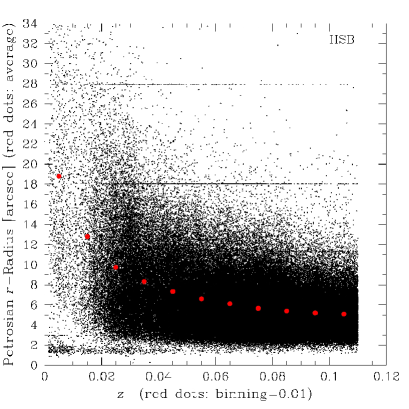
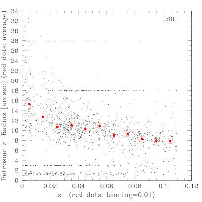
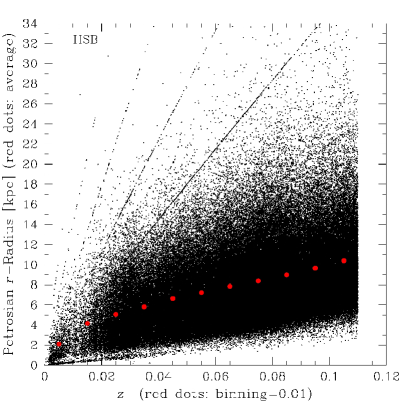
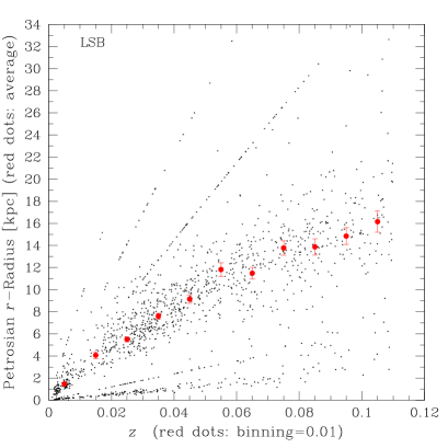
Figure 2: The left upper panel shows the distribution of the apparent Petrosian-$r$ radius (in arcsec) against redshift $z$ of HSB sample galaxies (black dots). Red dots are the average Petrosian radii (in arcsec) within redshift bins with a bin width of 0.01. The statistical error has a typical value of 0.07 arcsec and is therewith smaller than the size of the red points. Right upper panel shows the same as left upper panel, but for the LSB sample galaxies. Here, error bars indicate the statistical error of the indiviual average. Mind, that for a redshift of $z>0.01$ the LSB galaxies are larger in apparent radius than the HSBs. The statistical error is smaller than the size of the red points. At the lower left panel the distribution of the absolute Petrosian-$r$ radius (in kpc) versus the redshift $z$ is displayed for HSB galaxies. The average of the distribution within redshift bins of 0.01 is shown as red dots. The typical value for the statistical error of these averages is 0.03 kpc. Therewith it is smaller than the size of the points. The lower right panel shows the same diagram as the lower left panel, but for LSB galaxies. Error bars indicate the statistical error of the individual average values. Mind, that with increasing $z$ the averaged absolute Petrosian size of the galaxies also grows in both the HSB and LSB case.

It is conspicuous that for the redshift interval of $0.01<z<0.055$ the diagram shows a LSB galaxy population which is dominated by dwarf-like galaxies. The mean value of the absolute magnitude distribution in this redshift interval is $\overline{M}_{B}=-16.58\pm 0.08$ mag. The peak of the distribution lies at a value of $\sim-18.0$ mag. These value places the dominant LSB galaxy population of the redshift interval of $0.01<z<0.055$ into a region of dwarf-like, irregular galaxies and small spirals in the galaxy luminosity distribution. The average value is similar to the luminosity of the Small Magellanic Cloud ($M_{B}=-16.5$ mag, van den Bergh 2000), the peak value is similar to that of the Large Magellanic Cloud ($M_{B}=-18.0$ mag, van den Bergh 2000).

For the higher redshift interval with $0.055<z<0.1$ the situation changes. The peak of the distribution migrates towards the brighter region of the absolute magnitude diagram in comparison to the other redshift interval. This means that there the LSB population is dominated by larger, more massive galaxies. This is confirmed by the mean values of the distributions. A mean value of $\overline{M}_{B}=-18.13\pm 0.10$ mag was calculated. This value is similar to that of the Large Magellanic Cloud ($M_{B}=-18.0$ mag, van den Bergh 2000). The peak of the distribution is located at a value of $\sim$-19.3 mag (which is similar to that of M 33). This also places these galaxies in the total magnitude range of HSB spiral galaxies.

The lack of low-luminosity LSB galaxies at the higher redshift interval is not caused by dimming effects since the Petrosian magnitude is free from cosmological dimming effects (Section 2). It is obvious that this lack is caused by the apparent Petrosian $r$-magnitude limit of $r<17.77$ mag. It causes smaller galaxies with a low absolute magnitude to be excluded from spectroscopic targeting at the higher redshift interval. For example, a galaxy with a total absolute $r$-magnitude of $M_{r}=-17.50$ mag at a redshift of $z=0.055$ has an apparent magnitude of $m_{r}$=19.30 mag and therefore it would be excluded from spectroscopic targeting by the magnitude limit, unless the field is sparse populated so that there are still fibers left after the application of the strict criterias for spectroscopic targets.

More puzzling than the absence of dwarfish galaxies at the higher redshift interval of $0.055<z<0.1$ is the apparent lack of large LSBs at lower redshifts of $0.01<z<0.055$. Indeed, it is not the case that there are no large galaxies in the lower redshift interval of $0.01<z<0.055$, but they are overwhelmed by small galaxies. This effect is not only observed for LSBs but also for HSB galaxies of the SDSS sample. This is seen in Figure 2.

The upper left panel of the figure shows the angular Petrosian-$r$ radius in arcsec versus the redshift of the galaxy for all HSBs. At the upper right panel, the same is shown for LSBs. Red dots are the mean values of the apparent Petrosian-$r$ radius distribution within the corresponding redshift interval, in the upper left panel for HSBs and in the upper right panel for LSB galaxies. The binning of the redshift intervals is $\Delta z=0.01$.

The distribution of the average angular Petrosian-$r$ radius of both galaxy types (in both upper panels) is quite flat. For HSBs (left upper panel) the average apparent Petrosian-$r$ radius declines by $\sim 60\%$ between the redshift of $z=0.01$ and $z=0.1$, whereas the comoving distance (the distance obtained from redshift by assuming Hubble flow) is increased tenfold.

A similar situation is found in the LSB data. The averaged distribution of the angular Petrosian radius (red dots in the right upper panel) shows the same declining trend as for HSBs between a redshift of $z=0.01$ and $z=0.1$ but the average apparent radius is only decreased by $\sim 40\%$ within that redshift range. In both diagrams there are three horizontal line-like structures. These lines are artefacts due to a bug of the SDSS pipeline, since it was checked by eye that all objects forming a line in that diagram do definitively not have the same angular size. The problem is known by the SDSS pipeline programmers and it is caused by the “mismatches between the spectroscopic and imaging data”. On the DR4 homepage it is stated that for various reasons, a small fraction of the spectroscopic objects do not have a counterpart in the best object catalogs. In addition, the DR4 does not contain photometric information for some of the special plates, and the retrieval of photometric data from the CAS database requires special care for objects from the special plates (see also: www.sdss.org/dr4/start/aboutdr4.html).

The lower panels show the Petrosian radii in kpc calculated from the angular size and the comoving distance obtained from redshift (left panel for HSBs, right panel for LSBs). Since the data are not corrected for Virgocentric infall the comoving distances and therewith the calculated radii are accurate only for redshifts beyond $z=0.01$. For HSBs the average apparent Petrosian radius decreases by a factor of $\sim 2.5$ between redshift $z=0.01$ and $z=0.1$, but the redshift increases by a factor of ten, the average absolute Petrosian radius also increases. It does not grow linearly with a factor of four but with a factor of 2.5, since the comoving distance is not directly linear with $z$ due to relativistic corrections. The situation for LSBs (lower right panel) is similar, again. The averaged absolute Petrosian radius also rises between a redshift of $z=0.01$ and $z=0.1$ with a slope of $\sim 4$. This is caused by a decreasing angular radius with a slope of about 5/3 within a redshift range from $z=0.01$ to $z=0.1$ but a comoving distance increased by a factor of ten, minus relativistic corrections. Both the HSB and LSB lower diagram also show artefacts which are the same artefacts as in the upper panels but now producing diagonal lines due to the calculation of the absolute Petrosian radii by calculating the comoving distances from the redshifts.

This effect seen in the diagrams of Figure 2, that with increasing distance on average larger galaxies are sampled, is mainly caused by the apparent magnitude limit for spectroscopic follow up of Petrosian $m_{r}\leq 17.77$ mag. For reaching this magnitude limit galaxies at higher distances must of cause be larger and therewith more luminous in total absolute magnitude.

The fact that the sample LSBs must be larger than their HSB equivalents to reach this limit due to their low stellar surface densities is obvious. From this it is clear that at lower redshifts, both the LSB and the HSB sample are dominated by dwarfish galaxies, but at higher redshifts these galaxies do not get over the magnitude limit. The $m_{r}\leq 17.77$ mag limit is not a sharp criterion, because in case that not all fibers are used for bright galaxies free fibers are assigned to galaxies which are below that limit. However, this case is rare. Nevertheless, a sparse population of dwarfish galaxies is sampled at higher redshifts as well.

After understanding the SDSS selection function we were able to start examinating the environment of LSB galaxies. Furthermore, the selection function gives the possibility to switch the probed LSB galaxy population between a sample consisting of large LSBs and another sample dominated by smaller LSBs just by changing the redshift interval. Moreover, the HSB comparison sample can also be changed between a sample also containing smaller galaxies and a sample without small galaxies.

3 Results: The Environment of LSBs

The data for the environment studies were obtained from the main galaxy sample of the SDSS DR4. As described above, a redshift limit of $z\leq 0.11$ was applied. Thereby, a sufficient accuracy for the redshift of 30 km/s was achieved by demanding a $z$-confidence of more than 90%. Galaxies with a central, Tolman-dimming corrected surface brightness of $\mu_{B}\geq 22.5$ mag/arcsec² were flagged as LSB galaxies, otherwise they were flagged as HSBs. Thereby the central $B$-surface brightness was obtained by fitting exponential profiles (equation 1) to the azimuthally averaged surface brightness profiles measured by the SDSS pipelines and the central surface brightnesses in the SDSS modified Gunn bands $g$ and $r$ which were converted into a $B$-surface brightness using the transformation equations of Smith et al. (2002).

The uncertainty of the central surface brightness obtained from fitting surface brightness profiles to the surface-brightness distribution of each galaxy produces false classified galaxies in both the HSB and LSB bin. To estimate the number of false classified HSBs that contaminate the LBS bin Monte-Carlo simulations on the surface-brightness distribution were performed. Therefore the obtained distribution in central surface brightness of all galaxies was convolved with an Gaussian distribution representing the uncertainty in the central surface brightness. With a typical value of about $0.1$ mag/arcsec² for this uncertainty (standard deviation) in the central surface brightness the amount of intrinsically HSBs pushed into the LSB bin spuriously and vice versa was determined. We found the number of HSBs spuriously classified as LSBs to be 13% of the total amount of galaxies in the LSB bin. Therefore the LSB sample is contaminated with 13% of falsly classified HSBs. Coevally, the simulation shows that 5% of true LSBs are shifted into the HSB bin due to this uncertainty in central surface brightness. Therefore we conclude the LSB sample to contain an adequate number of true LSBs for performing environment studies on LSBs as described in the following.

In order to probe the environment of the LSB galaxies one has to count neighbor galaxies using a certain search volume. It is clear, that as a neighbor both LSB and HSB galaxies count. Additionally, the galaxy density in the vicinity of LSBs was compared to the galaxy density in the vicinity of HSBs. For these two reasons, the LSB and HSB galaxies were stored into one file, but with different flags indicating LSB or HSB property. Hence, and with an appropriate neighborhood analysis code, it was guaranteed that as neighbor of a scrutinized LSB galaxy (and of course a HSB) both LSB and HSB galaxies count for indicating the surrounding galaxy density.

3.1 The Pie Slice

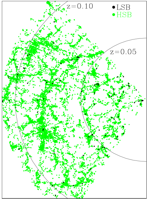
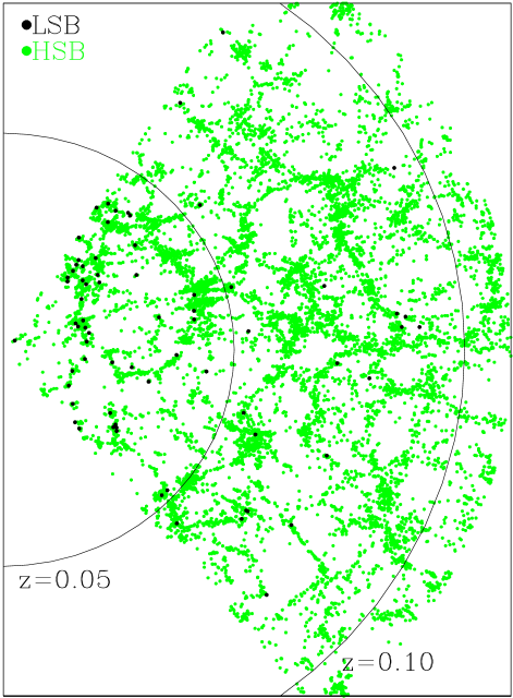
Figure 3: Two analyzed pie slices produced from SDSS DR4. Black dots are LSB galaxies and green dots represent HSBs. Left panel shows the distribution of LSBs and HSBs within a right ascension range of 120°$\leq\alpha_{2000}\leq 240$° and a redshift of $z\leq 0.11$ in a polar plot. The declination range of -1.25°$\leq\delta_{2000}\leq 1.25$° is projected onto the plane. Right panel shows the same, but for a right ascension range of 310°$\leq\alpha_{2000}\leq 360$°  and 0°$<\alpha_{2000}\leq 60$°. The declination range is again -1.25°$\leq\delta_{2000}\leq 1.25$°. Mind, that within a redshift interval of $0.05\leq z\leq 0.11$ the LSBs are mainly located at the outer parts of the filaments and walls of the LSS defined by HSBs. However, for a redshift of $z<0.05$ the situation is not so clear. There one can find LSB galaxies at the outer parts of the filaments as well as in the middle of walls and clusters. Thereby, one has to take into account that at the lower redshift interval the LSB population is dominated by dwarfish galaxies and at higher redshifts the LSB sample mainly consists of larger galaxies.

For a first glance at the distribution of the LSB galaxies within the large-scale structure (LSS), so called pie slices were plotted from the database obtained as described in the section before. Figure 3 shows such pie slice diagrams, where the distribution of right ascension and the redshift of LSB (black dots) and HSB galaxies (green dots) are displayed in polar plots. The left panel contains the right ascension range which was taken from an equatorial scan region of the DR4 with 120°$\leq\alpha_{2000}\leq 240$°  and the declination range of -1.25°$\leq\delta\leq 1.25$°  is projected onto the plane, whereas the redshift is limited to a value of $z\leq 0.11$. The right panel shows a pie slice of the same declination range, but with a right ascension of 310°$\leq\alpha_{2000}\leq 360$°  and 0°$<\alpha_{2000}\leq 60$°. The left panel contains 94 LSBs and 12768 HSBs, the numbers for the right panel are 72 LSBs and 11379 HSBs.

3.2 Neighbor Counting within Spheres

In order to quantify the differences in the surrounding galaxy densities of LSBs with respect to that of HSBs statistical neighbor counting was performed.

3.2.1 The Neighbor Counting Algorithm

For this analysis, an algorithm for counting neighbors was developed. This algorithm works as follows. For each galaxy, a sphere with a certain radius is defined with the probed galaxy in the center. Then the number of neighbor galaxies within this sphere is counted. This step is performed for all galaxies found in the program input file. Since the data of LSB and HSB galaxies are stored in one file which is used as the data input for the program, both galaxy types count as neighbors independent from if the scrutinized galaxy is a LSB or HSB. The radius of the sphere is an input parameter which the user is asked to define at the program start, as well as the names of the input and output files. After the interrogation of the input parameter and files, the program calculates for each galaxy of the input file the comoving distances by applying a Hubble constant of 71 kms^-1Mpc^-1 (Spergel et al., 2003) and the speed of light. Thereby, relativistic corrections for the redshifts were used. Since the environment studies were limited to a reshift range of $0.01\leq z\leq 0.1$, neither Virgocentric infall was corrected nor more complicated streaming motions than pure Hubble flow was taken into account. After that the right ascension, declination, and comoving distances are converted into Carthesian coordinates. Then the code starts neighbor counting within the 3-dimensional distribution of LSB and HSB galaxies by centering a sphere with a radius which was specified at program startup on each galaxy of the input file and then counting the neighboring galaxies within this sphere.

In order not to distort the statistical results at the borders of the catalogue volume, an edge correction was applied. The borders of the sample were avoided so that galaxies whose spheres were cutting the edges of the sample volume were rejected and not stored in the output file. Since all galaxies in the input file are HSB or LSB type flagged, one has the possibility to divide the result into statistics for the environment of LSBs and HSBs separately. For edge correction the covered volume of the input catalog was sampled with cubes of different sizes which did not cut the borders of the catalog.

Due to the fact that at lower redshifts ($0.01\leq z\leq 0.055$) the sample LSBs are dominated by dwarfish galaxies and at higher redshifts ($0.055\leq z\leq 0.1$) mostly large galaxies are contained in the LSB sample, the environment study had to be separated into these two redshift intervals. For each redshift interval, the environment studies were performed in different runs with several values for the sphere radius. It was varied from 0.8 Mpc to 8 Mpc in steps of 0.6 Mpc. The lower border of the scale range (0.8 Mpc) was chosen to avoid bias effects to the statistics caused by fiber placement constraints, since the minimum possible distance between two adjacent fibers is 55” in angular distance. This value corresponds to a minimum distance between two adjacent galaxies of 0.112 Mpc at a redshift of $z=0.1$ for getting spectra of both galaxies. Hence, with a sphere radius of $r=0.8$ Mpc, effects caused by fiber placement constraints are well sampled.

The upper border of the scale range (8 Mpc) of the neighbor counting was chosen, because with higher values the probed volume decreases due to boundary corrections and the statistics drops in significance. However, the chosen scale range is sufficient to probe the spatial distribution of LSBs on group radius scales (1-3 Mpc, Cox 2000; Krusch 2003) and filament sizes ($\sim 5$ Mpc, e.g. White et al. 1987; Doroshkevich et al. 1997).

3.2.2 The Galaxy Cluster Finding Algorithm

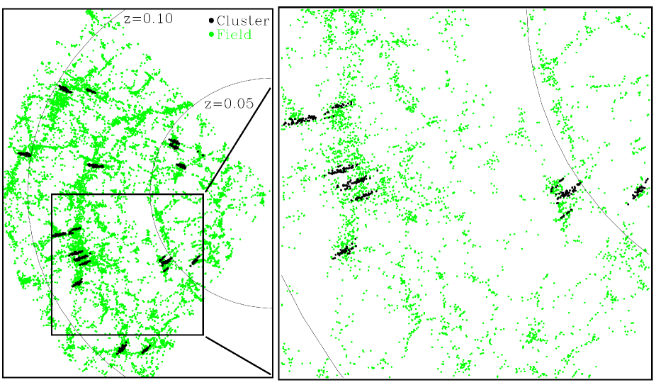
Figure 4: Pie slice to demonstrate the cluster finding algorithm. The left diagram shows the distribution of all HSB galaxies within a right ascension range of 120°$\leq\alpha_{2000}\leq 240$° and a redshift of $z\leq 0.11$ in a polar plot. The declination range of -1.25°$\leq\delta_{2000}\leq 1.25$° is projected onto the plane. The galaxies found to be arranged in clusters detected by the cluster finding algorithm are marked with black dots, whereas the field galaxies are displayed as green dots. It can be seen, that the cluster searching code finds the “finger of god”-like structures in the LSS. Additionally, these plots show that all clusters are embedded in wall-like structures of the LSS which indicates that the structure formation has not been completed, yet.

After the analysis using the code for neighbor counting, cluster galaxies had to be excluded from the sample in a second statistical analysis for a comparison of the clustering properties of field LSBs and HSBs. This was done due to the fact that, when calculating comoving distances from redshifts, the velocity dispersion (which can exceed values of $\sigma\geq 1000$ km/s) of galaxy clusters mocks an extension of the cluster in the line of sight direction. These structures bias the results in the LSS and had to be removed from the data. Therefore, an algorithm for finding clusters was developed.

This algorithm searches for clusters in the LSS by counting galaxies within a cylinder aligned radially in the line of sight direction with a configurable radius and height. The radius $r$ of the cylinder thereby complies with the radius of the cluster and the height of the cylinder corresponds to its velocity dispersion $\sigma$. These two values are parameters which can be chosen by the user of the program. The minimum number of cluster members ($N_{members}$) can also be set at program startup.

In a parameter study, the best parameters concerning $r$, $\sigma$, and $N_{members}$ for finding galaxy clusters were figured out. It turned out that, the best results of the hunt for galaxy clusters producing “fingers of god” were achieved with the parameters cylinder radius $r=2.5$ Mpc, velocity dispersion $\sigma=1000$ km/s and the minimum number of cluster galaxies $N_{members}=50$. Our cluster search code is based on a definition similar to the definition used by Abell (1958) and Abell et al. (1989), but it works in three dimensions. They defined the galaxy clusters mainly by a richness and a compactness criterion. The richness criterion requires that, a cluster must contain at least 50 members that are not more than 2 mag fainter than the third brightest member. In the compactness criterion it is demanded that a cluster must be sufficiently compact that its 50 or more members are within a given radial distance $r$ of its center.

The cluster finding algorithm was applied to the catalog containing the DR4 LSB and HSB sample after the neighbor counting within spheres. The program produced a file containing all (LSB and HSB) galaxies of the input files except the cluster galaxies of the clusters found by the program. This means that the cluster galaxies were removed from the galaxy sample file (containing neighborhood informations) retroactively, which means that only the distribution of field galaxies flows into the statistic. Otherwise, if one performs the cluster removal before environment analysis, one would produce holes into the large-scale structure which had to be masked out before the environment analysis. If not masked out, they would distort the statistics like boundary effects (which were also excluded).

3.2.3 The resulting LSB Environment

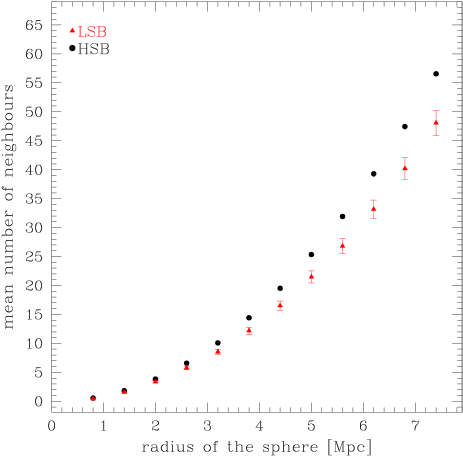
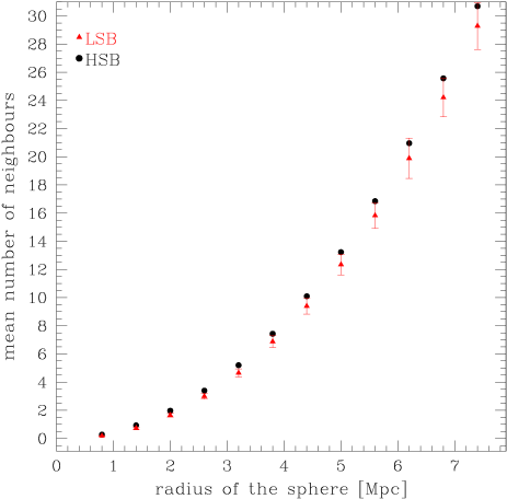
Figure 5: The diagrams show the average number of neighbors for LSBs (red triangles) and HSBs (black dots) versus the radius of the sphere within which the neighbors were counted. Both plots are not corrected for cluster galaxies. Left diagram displays the results of the redshift interval of $0.01\leq z\leq 0.055$, right panel shows the same but for the redshift range of $0.055\leq z\leq 0.1$. The average number of neighbors stays for LSBs systematically below the values of the HSB statistics both for the lower redshift interval (left) and the higher redshift interval (right).

During several runs of the neighbor counting algorithms as described above, the radius of the sphere was varied between 0.8 Mpc and 8.0 Mpc in steps of 0.6 Mpc. The number of neighbors of each individual run of the program (with a fixed sphere radius) were averaged for LSB and HSB galaxies. Because of the SDSS selection function the sample contains LSB galaxies of different size and total luminosity at different redshifts, namely the low redshift interval of $0.01\leq z\leq 0.055$ is dominated by dwarfish LSBs. The higher redshift range of $0.055\leq z\leq 0.1$ contains mainly large LSBs. Therefore the examinations on the environment were divided into two symmetric redshift bins corresponding to these redshift intervals.

Figure 5 shows the average number of neighbors for LSBs (red) and HSBs (black) versus the sphere radii within the redshift intervals $0.01\leq z\leq 0.055$ (left panel) and $0.055\leq z\leq 0.1$ (right panel). To produce this diagram neighbor counting was performed in several runs within spheres with radii between 0.8 Mpc and 8 Mpc in steps of 0.6 Mpc. For each sphere radius the number of neighbors was averaged for the LSB galaxies and for the HSB galaxies (as neighbor both galaxy types counted). In the lower redshift interval $\sim 400$ LSBs were probed in comparison to $\sim 31000$ HSBs. For the higher redshift interval the sample contains $\sim 200$ LSB and $\sim 69000$ HSB galaxies. In this case, cluster correction was not applied to the data. The data show that LSB galaxies have on average less neighbors than HSB galaxies on scales between 0.8 Mpc and 8.0 Mpc. This is the case for both redshift intervals (although the trend is less significant in the higher redshift interval). This means that dwarfish LSBs as well as large LSBs are preferably found in regions with lower galaxy density than in the vicinity of HSBs. The next step was to probe the location of LSBs in the LSS without clusters. For that, the cluster galaxies were removed from the statistics using the cluster finding algorithm (section 3.2.2). This means, that all galaxies, which are located in a LSS volume occupied by a cluster, were removed from the statistics that it was averaged over pure field galaxies. Figure 6 shows the results of that study. Again, two redshift bins (left panel: $0.01\leq z\leq 0.055$, right: $0.055\leq z\leq 0.1$) were examined. Galaxies which have more than 50 neighbors within a cylinder with a radius of 3 Mpc and a height of 1000 km/s aligned with its axis towards the line of sight were rejected. Again, the number of neighbors were averaged for LSBs and HSBs at different sphere radii. The diagrams show that on average LSB galaxies have less neighbors than HSB galaxies on all probed scales for both dwarfish and large LSB galaxies, since all triangles representing the average LSB number of neighbors are located systematically below the corresponding averaged values for HSBs. For the redshift bin with $0.01\leq z\leq 0.055$ (left panel) it becomes statistically significant at a sphere radius of 3.2 Mpc. For the higher redshift bin (with $0.055\leq z\leq 0.1$, right panel) it is statistically significant between 2 Mpc and 3.8 Mpc. As all LSB values are located below the HSB values, one can argue that the effect is also seen on scales with lower statistical significance, since the probability is small that all LSB points are located below the HSB values due to statistical noise.

The statistical significance of the statement that LSB galaxies have on average less neighbors than HSBs had to be probed. For that, Kolmogorov-Smirnov (KS, Chakravarti et al. 1967) two sample tests were performed on the LSB and HSB distribution of neighbors from which the average values were calculated. The KS test is intended to probe the null hypothesis that two data samples come from the same distribution. Since the KS statistic is used for unbinned data sets, it was applied to the unbinned number of neighbor distribution of LSBs forming the first data sample and the same distribution for HSBs producing the second test data sample.

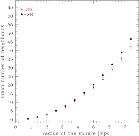
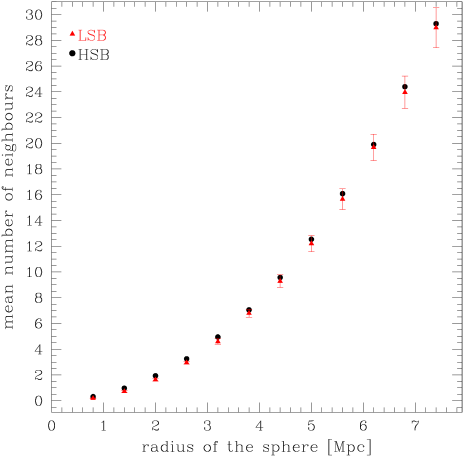
Figure 6: The panels show again the average number of neighbors for LSBs (red triangles) and HSBs (black dots) versus the sphere radius within the two redshift intervals (left: $0.01\leq z\leq 0.055$, right: $0.055\leq z\leq 0.1$), but at this time the cluster galaxies were removed from the statistics (as described in section 3.2.2). This means that the distribution of LSBs in comparison to HSBs was probed in the field. On average the LSB galaxies still have less neighbors than HSBs but the signal is not so strong (but still significant) as if we average over cluster and field galaxies (Figure 5).

The results are presented in Table 1 and 2. Thereby, Table 1 refers to the significance of the null hypothesis in Figure 5 with respect to the corresponding scale radii. This Figure contains statistics including both cluster and field galaxies. For the lower redshift range with $0.01\leq z<0.055$ (Figure 5, left diagram), our hypothesis that LSB galaxies have on average less neighbors than HSBs holds with more than $1\,\sigma$ probability for the scale range of 0.1 Mpc to 2.6 Mpc and with around $2\,\sigma$ probability for scales between 3.2 Mpc and 5.0 Mpc. For the scale interval of 5.6 Mpc to 8.0 Mpc, a significance of around 3 $\sigma$ is reached for this hypothesis.

In this context, one should take into account the selection function for LSBs (Figure 1), which shows that this scrutinized redshift range is dominated by dwarfish LSB galaxies. Then, this result shows that there exists a density contrast for small LSBs, which are on average located in a less dense environment than field and cluster HSBs. In diagram 5 (right panel) this hypothesis holds with explicitly more than $1\,\sigma$ significance for values of the sphere radii between 0.8 Mpc and 2.0 Mpc. For the scale values of 2.6 Mpc and 3.2 Mpc the probability of the hypothesis is still around $1\,\sigma$, but it drops below the value for higher scale radii. However, all LSB neighboring values in Figure 5 (right) at that scales are located systematically below the average number of neighbors for HSBs. This indicates that this effect is real with a higher probability and over a larger range of radii than the KS test indicates.

Table 1: Significance of neighbor counting statistics

Significance of Statistics
z-range / refers to Figure	radius [Mpc]	significance [%]
$0.01\leq z<0.055$	0.8	91.38
Figure 5 (left)	1.4	90.71
not cluster corrected	2.0	74.23
	2.6	69.11
	3.2	94.25
	3.8	91.16
	4.4	94.37
	5.0	97.88
	5.6	99.26
	6.2	99.01
	6.8	98.55
	7.4	99.93
	8.0	99.48
$0.055\leq z<0.1$	0.8	79.26
Figure 5 (right)	1.4	91.51
not cluster corrected	2.0	79.77
	2.6	64.48
	3.2	64.66
	3.8	52.17
	4.4	47.61
	5.0	55.95
	5.6	57.57
	6.2	34.50
	6.8	40.86
	7.4	44.38
	8.0	33.27

Table 2: Significance of neighbor counting statistics continued

Significance of Statistics
z-range / refers to Figure	radius [Mpc]	significance [%]
$0.01\leq z<0.055$	0.8	70.22
Figure 6 (left)	1.4	69.24
cluster corrected	2.0	49.12
	2.6	56.81
	3.2	84.08
	3.8	77.84
	4.4	87.88
	5.0	95.06
	5.6	98.18
	6.2	97.63
	6.8	96.73
	7.4	97.39
	8.0	98.67
$0.055\leq z<0.1$	0.8	68.80
Figure 6 (right)	1.4	86.59
cluster corrected	2.0	64.36
	2.6	41.88
	3.2	41.57
	3.8	27.71
	4.4	37.05
	5.0	35.56
	5.6	38.55
	6.2	16.07
	6.8	21.55
	7.4	23.97
	8.0	16.41

Table 2 refers to the Figure 6 and gives probabilities that the (inverted) null hypothesis that LSB galaxies have less neighbors than field HSBs is true on different scales for two redshift intervals. Figure 6 contains the comparison between field LSB galaxies and field HSBs, since all cluster galaxies were removed from statistics.

For the redshift range of $0.01\leq z<0.055$ the following situation turns out to be as follows. For the scale values of 0.8 Mpc and 1.4 Mpc this hypothesis holds with more than $1\,\sigma$ significance. The sphere radii of 2.0 Mpc and 2.6 Mpc have a probability of around 50% for the trueness of the hypothesis. On scales between 3.2 Mpc and 4.4 Mpc the statement possess clearly more than $1\,\sigma$ probability. And for the sphere range of 5.0 Mpc to 8.0 Mpc the significance is with values of $2\,\sigma$ up to $3\,\sigma$ quite high.

For the higher redshift interval with $0.055\leq z<0.1$ the situation is not clear. The first three scale values with 0.8 Mpc, 1.4 Mpc and 2.0 Mpc have a significance for the hypothesis of around and about $1\,\sigma$. However, the probability that the hypothesis holds at higher sphere radii is low, below 50%. Since the number of neighbors is on average still lower for LSBs than for HSBs, this might be a hint that a difference in the LSB and HSB environment might exist in this redshift bin as well. However, when considering each value in diagram 6 (right) individually, the density contrast is not significant on scales of 2.6 Mpc and above. This is an effect of small numbers, which will be improved with further data sets covering larger sky areas.

3.3 LSB-HSB Antibias

In order to find another independent method to quantify the clustering properties of LSBs in comparison to HSBs, the LSB-HSB biasing parameter was derived from the SDSS dataset. The galaxy bias is a term from cosmology and is normally used to describe the difference in the clustering properties between galaxies and Dark Matter on large scales. We use this stochastic bias measure for the first time to display differences in the clustering properties of LSBs in comparison to HSBs. The LSB-HSB Antibias parameter was derived from the Neighbor Counting Analysis as described before by using the galaxy number density $N$ at the location of each galaxy within spheres of the radius $R$. The second moment of the density contrast was then calculated for the density field at the location of all sample LSBs and HSBs using the equations

$$<\delta_{R,\rm LSB}^{2}>\,=\frac{1}{n}\sum_{i=1}^{n}\left(\frac{N_{i,R,\rm LSB}}{\overline{N}_{R,\rm LSB}}-1\right)^{2},$$ (2)

and

$$<\delta_{R,\rm HSB}^{2}>\,=\frac{1}{n}\sum_{i=1}^{n}\left(\frac{N_{i,R,\rm HSB}}{\overline{N}_{i,R,\rm HSB}}-1\right)^{2}.$$ (3)

Using these equations (2, 3) in combination with the results of the environment studies within spheres of the radius $R$, the average density contrast at the locations of LSBs and the same quantity at the locations of HSBs were calculated. Thereby, $N_{i,R,\rm LSB}$ is the number of (LSB and HSB) galaxies within a sphere of the radius $R$ centered on the LSB galaxy $i$ or expressed in a different way the galaxy number density within a radius $R$ at the location of the $i^{\rm th}$ LSB galaxy. The quantity $n$ is the total number of LSBs in eq. 2 (or HSBs in eq. 3) and $\overline{N}$ is the number of (LSB and HSB) galaxies within that radius $R$ averaged over all LSB galaxies.

From these results, the stochastic bias parameter $b(R)$ was obtained using the following equation

$$b(R)=\sqrt{\frac{<\delta_{R,\rm LSB}^{2}>}{<\delta_{R,\rm HSB}^{2}>}},$$ (4)

with $R$ the sphere radius, $<\delta_{R,\rm LSB}^{2}>$ the second moment of the LSB density contrast in dependence of the radius of the probing sphere and $<\delta_{R,\rm HSB}^{2}>$ the same but for the sample HSB galaxies.

With the definition of this parameter it is now possible to express the differences in the LSB and HSB environment in terms of the density contrast and galaxy bias.

3.3.1 Results on the LSB-HSB Antibias

The results obtained from probing the LSB-HSB galaxy bias are presented in Table 3. In that Table, the values for the second moment of the density contrast for LSBs calculated using 2, for HSBs (equation 3), and the resulting values for the LSB-HSB bias parameter calculated from equation 4 are given. These values are displayed in dependence on the sphere radius. The results are again divided into the two redshift bins as used several times before. Furthermore, a division of the results into the cases “not cluster corrected” and “cluster corrected” is done. The first case probes the LSB galaxy bias with respect to all (field and cluster) HSBs. The second case tests if the distribution of LSB galaxies is biased against field LSBs.

Table 3: LSB-HSB galaxy bias parameter

LSB-HSB Galaxy Bias
redshift: $0.01\leq z<0.055$ / not cluster corrected
$R$ [Mpc]	$<\delta_{R,\rm LSB}^{2}>$	$<\delta_{R,\rm HSB}^{2}>$	$b(R)$
8.0	0.798	1.039	0.876
5.6	0.912	1.256	0.852
3.2	1.081	1.460	0.861
redshift: $0.055\leq z<0.1$ / not cluster corrected
$R$ [Mpc]	$<\delta_{R,\rm LSB}^{2}>$	$<\delta_{R,\rm HSB}^{2}>$	$b(R)$
8.0	0.612	0.745	0.906
5.6	0.643	0.835	0.877
3.2	0.769	1.026	0.866
redshift: $0.01\leq z<0.055$ / cluster corrected
$R$ [Mpc]	$<\delta_{R,\rm LSB}^{2}>$	$<\delta_{R,\rm HSB}^{2}>$	$b(R)$
8.0	0.600	0.596	1.002
5.6	0.649	0.655	0.994
3.2	0.799	0.782	1.009
redshift: $0.055\leq z<0.1$ / cluster corrected
$R$ [Mpc]	$<\delta_{R,\rm LSB}^{2}>$	$<\delta_{R,\rm HSB}^{2}>$	$b(R)$
8.0	0.607	0.705	0.927
5.6	0.637	0.775	0.906
3.2	0.756	0.931	0.902

For these particular cases the variance of the density contrast and the LSB-HSB bias parameter were calculated from environment studies with spheres of the radius 8.0 Mpc, 5.6 Mpc and 3.2 Mpc. The first value of $R=8.0$ Mpc was chosen to compare the averaged squared density contrast directly with $\sigma_{8}$ from results obtained by other redshift surveys in the literature. $R=5.6$ Mpc probes the LSB-HSB bias on scales of the size of large scale structure filaments ($\sim 5$ Mpc, e.g. White et al. 1987; Doroshkevich et al. 1997). The value of $R=3.2$ Mpc was selected for testing the LSB-HSB clustering on scales of the diameter of clusters. Furthermore, this radius under-samples the averaged size of filaments only marginally. Therefore, it can be used to support the results obtained from the bias study of $R=5.6$ Mpc concerning the filaments, which of course also shows structure on scales of $R=3.2$ Mpc. It is not reasonable to calculate the bias using studies based on spheres with smaller radii, because using spheres of a radius $R$ means that the local galaxy density is averaged over a sphere of the radius $R$. If the radius is chosen too small, the fluctuations of the density from galaxy to galaxy get too high. Since the bias is a measure of fluctuations, the study is less meaningful when choosing lower values for $R$. This can also be explained in another way. The radius $R$ of the sphere is a kind of smoothing parameter for the density field. If one chooses this parameter to be low, the smoothing effect is too low, and the noise overwhelms the signal. This effect can directly be seen in Table 3. For all cases and redshift ranges as well as for both galaxy types the variance of the density contrast increases with decreasing sphere radii.

For the study containing field and cluster galaxies within the redshift range of $0.055\leq z<0.1$ the density contrast for LSBs (equation 2) stays clearly below the value obtained for HSBs (obtained from equation 2) for both the cluster corrected case containing only field galaxies as well as the case containing cluster and field galaxies. This holds for all tested scales ($r=8.0,5.6,3.2$ Mpc). Thereby the density contrast for LSBs is below that value of HSBs indicating that LSBs are less strongly clustered than HSBs. This is also seen in the bias parameter $b$. For this redshift range it contains values between $b=0.906$ and $b=0.866$ for the cluster and field galaxy case and values in the interval of $b=0.927$ and $b=0.902$ for the case containing only field galaxies. These two cases do not differ a lot. This shows that the galaxy environment of LSBs within the redshift interval of $0.055\leq z<0.1$ is clearly less dense than that of HSBs for both the cluster corrected and not corrected case.

The first case shows a slightly smaller bias parameter than the case containing pure field galaxies. This is caused by the fact that clusters of course rise the variance of the density contrast. The sample LSBs are not often located in clusters (only one LSB of that redshift range was found in a cluster). This would explain the increased bias parameter in the case of pure field galaxies with respect to the case containing field and cluster galaxies. Nevertheless, the bias parameter holds below one for the comparison of the density contrast between field LSBs and field HSBs within that higher redshift interval. Taking into account the fact that the LSB population of that redshift range is dominated by larger LSBs, this gives strong evidence for a scenario in which the larger type LSBs formed and evolved in a lower density region than HSBs. Since there is still a lower density contrast for LSBs against that of HSBs in the cluster corrected case containing pure field galaxies, this gives strong support for the initial impression from the pie slice (Section 3.1). This impression was, that for the higher redshift interval $0.05<z<0.1$ the (larger) LSB galaxies are located at the outer rims of the LSS, and some of them are even found in void regions.

The examinations on the density contrast and bias parameter of LSB and HSB galaxies within the redshift range of $0.01\leq z<0.055$ delivered similar results except for the cluster corrected case. There, a difference in the density contrast between these two galaxy populations is not found. This results in a bias parameter of $b\sim 1$. Taking into account that the LSB population in this redshift range is dominated by small, dwarfish LSB galaxies, one can conclude that these galaxies are found in an environment which is more similar to that of HSBs. However, the average neighbor diagram of that case shows the presence of a density contrast (Figure 6, left).

In the case of cluster and field galaxies (and the same redshift interval of $0.01\leq z<0.055$), a significant difference in the density contrast with differences of $\sim 0.2$ up to $\sim 0.4$ are found. This results in a bias parameter of $b\sim 0.86$ indicating that these mainly smaller LSB galaxies do not have the same clustering properties like cluster and field HSBs combined.

All in all the galaxy bias study confirms the impression from the pie slice as well as the results of the mean number of neighbor diagrams (Figures 5, 6). From these studies follows that the vicinity of LSB galaxies indeed shows a lower galaxy number density than that of HSBs. This holds for the sample containing preferably larger LSBs as well as the small LSBs. We call this effect the “LSB-HSB Antibias”.

4 Discussion & Conclusions

As shown above, LSB galaxies reside in a large scale environment with a lower galaxy density than in the vicinity of HSBs. This was proved several ways. A first impression to that fact comes from the pie slice diagram 3. There, the impression aroused that LSBs in a redshift interval of $0.05<z<0.1$ are located at the outer parts of the filaments and walls. Some LSBs are even found in void regions of the LSS. The statistical analyses confirm this impression. For both redshift intervals ($0.01<z<0.055$ and $0.055<z<0.1$) it holds that LSBs possess less neighbors than HSBs (Figs. 5, 5, sections 3.2.3, 3.3). This is actually true, if one excludes cluster galaxies and only compares the environment of field LSBs to that of field HSBs. Even then a stronger isolation of LSBs is found.

First hints to that result already existed in the literature. Early results on the studies presented above were published in Rosenbaum & Bomans (2004). There it was shown that the LSBs found in the Early Data Release (EDR, Stoughton et al. 2002 of the SDSS possess a lower surrounding galaxy density than HSBs on scales from 2 to 5 Mpc. Other authors probed the environment of LSBs on intermediate and small scales. It was found that on scales below 2 Mpc, the galaxy environment of LSBs is less dense than that of HSBs (Bothun et al. 1993; Mo et al. 1994). Furthermore, a lack of nearby ($r\leq 0.5$ Mpc) companions of LSB galaxies was detected by Zaritsky & Lorrimer (1993). However, a study on the distribution of LSBs in the large-scale structure on scales which correspond to the size of its substructures (galaxy cluster radii $r\sim$1-3 Mpc, size of the LSS filaments and walls $\sim 5$ Mpc) has not been performed before.

All these results fit well into a formation scenario for LSBs proposed in Rosenbaum & Bomans (2004) which is based on an idea of Bothun et al. (1997). Galaxy formation takes place due to an initial Gaussian spectrum of density perturbations with much more low-density fluctuations than high density ones. Many of these low-density perturbations are lost because of the assimilation or disruption during the evolutionary process of galaxy formation but a substantial percentage of the fluctuations survives and is expected to form LSB galaxies. Further on one can assume that the spatial distribution of the initial density contrast consists of small scale fluctuations superimposed on large-scale peaks and valleys. Small-scale peaks lead to galaxy formation, whereas the large-scale maxima induce cluster and wall formation of the LSS.

If now galaxies formed in the large-scale valleys would develop to LSB galaxies because of their isolated environments whereas HSB galaxies would form mainly on the large-scale peaks this would lead to an universe with LSBs being more isolated than HSBs.

The isolation of LSB galaxies on intermediate and small scales must have effected their evolution since tidal encounters acting as triggers of star formation would have been rarer in these LSB galaxies than for HSB galaxies. Our results give strong evidence for this scenario, since the observed isolation of LSB galaxies takes place on scales of $\sim 5$ Mpc, which is the typical size of LSS filaments (e.g. White et al. 1987, Doroshkevich et al. 1997). Hence, LSB galaxies must have formed in the void regions of the LSS. After that, most of them have migrated to the edges of the filaments because of gravitational infall, but some of them still remain in the voids where they have formed in.

Another possible explanation for the presence of LSBs might be found in the differences in the spin parameter $\lambda$ of the Dark Matter halos between LSB and HSB galaxies. Dalcanton et al. (1997a) studied the formation of disk galaxies and used a gravitationally self-consistent model for the disk collapse in order to calculate the observable properties of disk galaxies as a function of mass and angular momentum of the initial protogalaxy. The observational properties of both normal galaxies and LSBs were reproduced. Their model generated smooth, asymptotically flat rotation curves and exponential surface brightness profiles. They found the high angular momentum halos, which also tended to be low mass, to form naturally low baryonic surface density disks or in other words low surface brightness disks. Boissier et al. (2003) found in their models for the chemical and spectrophotometric evolution of mainly spiral galaxies and LSBs, that the models with a spin parameter of $\lambda\sim 0.04$ corresponded to spirals with Freeman values of surface brightness. Moreover, models with $\lambda>0.06$ belonged to LSB galaxies. From these simulations follows that the Dark Matter halos of LSBs possess a higher spin parameter, than that of HSBs. Since, the spin parameter $\lambda$ is linked to the structural properties of the disk, this would imply a larger scale length for the LSB disks with respect to HSB disks. Hence, the total gas mass in LSBs would be distributed over a larger scale length than in HSBs. This would explain the lower gas surface density in LSBs, too.

However, these models for LSB formation do not necessarily contradict our formation scenario proposed above. Moreover, with the latest results of Bailin et al. (2005) it is possible to build a causal connection between this scenario described above and the results of simulations, that the larger extents of LSB Dark Matter halos result in a higher spin parameter. For these simulations it is assumed that the specific angular momentum of the baryons is conserved during their dissipation into a rotating disk (which is a reasonable assumption). Hence, the scale length of the disk would be related to the angular momentum of the Dark Matter halo. Therefore, a link would exist between the increased scale length and the concentration of their Dark Matter halos. Bailin et al. (2005) now performed a cosmological N-body simulation with $N=512^{3}$ on a periodic 50$h^{-1}$ Mpc volume using the GADGET2 code (by Springel 2005). Thereby, $\Lambda$CDM cosmology was assumed. The halos of a mass range of $10^{11}\leq M_{vir}/h^{-1}\leq 2\cdot 10^{12}$ which are typical to be hosts of LSB and HSB galaxies were identified using a friends-of-friends algorithm and the spin parameter $\lambda^{\prime}=J/[\sqrt{2}MVR]$ (with M, the total mass, J the total angular momentum, V the circular velocity at radius R) in a definition from Bullock et al. (2001) was calculated. As expected, a trend for $\lambda^{\prime}$ to increase with decreasing concentration index $c_{200}$ was found. For a concentration index of $c_{200}=10$, a median of the spin parameter $\lambda^{\prime}_{med}\simeq 0.03$ and for $c_{200}=5$ a value of $\lambda^{\prime}_{med}\simeq 0.05$ was obtained by the authors. Then, assuming angular momentum conservation of the baryons during dissipation into the rotating disk, the disk angular momentum and its extent for a given mass was calculated. From that, the central surface densities were estimated and the central surface brightnesses were estimated by using the fitting equations of Mo et al. (1998). At the end they found a clear trend that halos with lower concentrations host disks with lower central surface densities. With these results, for the first time a correlation between the spin parameter $\lambda^{\prime}$ and the concentration of the Dark Matter halos was found. The obtained results are not only important for the theories which predict the existence of LSBs to be caused by the higher spin parameter of Dark Matter halos. They are also important for the results of section 3.2.3, since this could be the connection between these two scenarios. The type of diffuse, less concentrated Dark Matter halos, which preferably host LSB galaxies, one would expect to exist in lower density regions, whereas the more concentrated Dark Matter halos one would expect to be formed in high density regions of the initial universe. This is compatible to the results of Avila-Reese et al. (2005), who performed $\Lambda$CDM N-body simulations. They found the halos in clusters to have a lower median spin parameter, to be more spherical, and to possess less aligned internal angular momentum than the halos in void or field regions. Their simulations showed trends that disk galaxies which formed in halos with low spin parameters, but high concentration indices, are preferably of earlier morphological types. Furthermore, these galaxies have higher surface brightnesses, smaller scale lengths, and lower gas fractions than galaxies formed in halos which have higher spin parameters, but are low-concentrated.

Hence, the results of Bailin et al. (2005) in combination with the simulations of Avila-Reese et al. (2005) and the results presented in the present publication answer the following question: Are LSB galaxies caused by nature or nurture? They exist due to a mixture of both.