Multipole Nonlinearity of Metamaterials

Abstract

We report on the linear and nonlinear optical response of metamaterials evoked by first and second order multipoles. The analytical ground on which our approach bases permits for new insights into the functionality of metamaterials. For the sake of clarity we focus here on a key geometry, namely the split-ring resonator, although the introduced formalism can be applied to arbitrary structures. We derive the equations that describe linear and nonlinear light propagation where special emphasis is put on second harmonic generation. This contribution basically aims at stretching versatile and existing concepts to describe light propagation in nonlinear media towards the realm of metamaterials.

I Introduction

Metamaterials are attracting much scientific interest due to their unique optical properties in terms of their tailorable effective material response and the potential exciting applications Pollard et al. (2009); Valentine et al. (2008); Pendry (2008); Cai et al. (2007). Most notably, the effective magnetic response is an extraordinary property that distinguishes metamaterials from all naturally available media at optical frequencies. It has been shown that the effective material properties, such as the effective magnetic and electric response, are determined by the resonant excitation of plasmonic eigemodes, dependending on the specific metaatom geometry Rockstuhl et al. (2006, 2007). Frequently the structure and physics of these eigenmodes is investigated by calculating the electric fields or currents inside the metaatom by powerful numerical techniques.
Here we present a more physical approach to characterize these eigenmodes by a multipole expansion up to the second order. This model permits for an analytical treatment of the light propagation in metamaterials at the expense that it constitutes merely a simplification of the real plasmon dynamics. Nevertheless, exactly for this reason the model provides unprecedented physical insights into the functionality of metamaterials which were inaccessible before by a pure numerical treatment. In the quasi-static approach for spherical or elliptical metal nanoparticles the fundamental plasmonic eigenmode is sufficiently described by an electric dipole. Metamaterials, which in general exhibit more complex geometries with an involved carrier dynamics, require to account for higher order multipoles as e.g. the electric quadrupole and the magnetic dipole moment representing the natural extension towards a fully electrodynamic model Esteban et al. (2008); Han et al. (2008). Furthermore the excitation of multipoles is frequently applied in order to explain the origin of the magnetic or the electric effective parameter response, phenomenologically. Here we present a coherent description corresponding to the way metamaterials are currently understood, namely by their multipole excitations. In particular, the simultaneous consideration of the magnetic dipole and the electric quadrupole is required by nature, since both occur in the same order of the multipole expansion. Though this has been extensively discussed in the literature Sharma (2007); David J. Cho et al. (2008); D Shin (2000); Guzatov et al. (2008); Petschulat et al. (2008); Pustovit et al. (2002), the quadrupole moment is frequently dropped.
Besides the linear properties that can be covered by this expansion we present the extension of the multipole description towards the quadratic nonlinear optical regime. Since the multipole expansion will be truncated beyond second order terms, we focus on the study of quadratic nonlinear effects associated with these second order multipoles. We mention that this procedure of introducing nonlinearity is known from the early works in nonlinear optics Bloembergen (1965); Pershan (1963) and is supported by several papers that observed multipole induced nonlinear optical effects in various plasmonic nanostructures Kujala et al. (2007); Bethune (1981); Bachelier et al. (2008); Jayabalan et al. (2008); Kim et al. (2008); Maluckov et al. (2008); Shadrivov et al. (2008a, b); Zharov et al. (2003).
Hence, the subject of this paper is twofold. At first we derive the required wave equations for the complete metamaterial system and compare the results (the dispersion relation, and the effective material parameters) in the linear limit with numerical calculations for a representative metaatom, i.e. the split-ring resonator (SRR). However, the formalism we introduce is general and can be straightforwardly applied to other geometries. The SRR was only chosen because first experiments on the second harmonic generation were already reported in this structure; though in a configuration amenable for nano-fabrication where the induced magnetic dipole is non-radiating Klein et al. (2006, 2007). To become specific in the second part second harmonic generation (SHG) in a SRR is studied in detail. In order to predict the second harmonic generation by purely analytical means, we finally apply the undepleted pump approximation (UDPA) and derive the associated equations within the multipole model. We observe an excellent agreement with the numerically derived solutions which justifies the application of this approximation for further predictions.

II The nonlinear wave equation

Our investigation starts with the wave equation incorporating multipoles up to second order Petschulat et al. (2008)

$$\Delta\mathbf{E}(\mathbf{r},t) = \mu_{0}\epsilon_{0}\frac{\partial^{2}}{\partial t^{2}}\mathbf{E}(\mathbf{r},t)+\mu_{0}\frac{\partial^{2}}{\partial t^{2}}\mathbf{P}(\mathbf{r},t)$$

$$- \mu_{0}\nabla\cdot\frac{\partial^{2}}{\partial t^{2}}\mathbf{\hat{Q}}(\mathbf{r},t)+\mu_{0}\nabla\times\frac{\partial}{\partial t}\mathbf{M}(\mathbf{r},t).$$

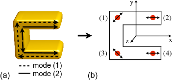
Figure 1: (a) SRR metaatom and the intrinsic currents for the fundamental electric (black solid line) and magnetic (black dashed line) mode. (b) The associated auxiliary charge distribution (red points) with predefined degrees of freedom (black arrows).

Now, in terms of the plasmonic eigenmodes of interest the respective metaatom has to be mapped onto the point multipoles: electric dipoles $\textbf{P}(\textbf{r},t)$, magnetic dipoles $\textbf{M}(\textbf{r},t)$ and electric quadrupoles $\mathbf{\hat{Q}}(\textbf{r},t)$. In order to observe both, an electric and a magnetic response, the SRR is uprightly oriented Rockstuhl et al. (2007), see FIG.(1). To cover the fundamental electric and magnetic modes Rockstuhl et al. (2006), sketched by the black solid and dashed lines in FIG.(1a), respectively, four auxiliary positive and negative charges with predefined spatial degrees of freedom are required as indicated in FIG.(1b). With the knowledge about these directional constraints for the carrier dynamics the microscopic definitions of the multipole moments can be applied as

$$\mathbf{P}(\mathbf{r},t) = \eta\sum_{l=1}^{N}q_{l}\mathbf{r}_{l}(\mathbf{r},t),$$ (2)

$$\mathbf{M}(\mathbf{r},t) = \frac{\eta}{2}\sum_{l=1}^{N}q_{l}\mathbf{r}_{l}(\mathbf{r},t)\times\frac{\partial}{\partial t}\mathbf{r}_{l}(\mathbf{r},t),$$

$$Q_{ij}(\mathbf{r},t) = \frac{\eta}{2}\sum_{l=1}^{N}q_{l}[\mathbf{r}_{l}(\mathbf{r},t)]_{i}[\mathbf{r}_{l}(\mathbf{r},t)]_{j},$$

where the equations of motion $\mathbf{r}_{l}(\mathbf{r},t)$ for each charge $q_{l}$ contain all information about the plasmonic eigenmodes. The parameter $\eta$ accounts for the dipole density. Even at this early stage it can be seen, that if $\mathbf{r}_{l}(\mathbf{r},t)\propto\mathbf{E}(\mathbf{r},t)$ second order multipoles will immediately evoke nonlinear contributions, since they involve terms $\propto\mathbf{r}_{l}^{2}(\mathbf{r},t)$. For the carrier configuration proposed here the associated terms $\mathbf{r}_{l}(\mathbf{r},t)$ are

$$\mathbf{r}^{+}_{1} = (-x_{0},y_{0},0),~{}\mathbf{r}^{-}_{1}=(-x_{0}-\xi_{1},y_{0}-\xi_{1},0),$$ (3)

$$\mathbf{r}^{+}_{2} = (x_{0},y_{0},0),~{}\mathbf{r}^{-}_{2}=(x_{0}-\xi_{1},y_{0},0),$$

$$\mathbf{r}^{+}_{3} = (-x_{0},-y_{0},0),~{}\mathbf{r}^{-}_{3}=(-x_{0}-\xi_{2},-y_{0}+\xi_{2},0),$$

$$\mathbf{r}^{+}_{4} = (x_{0},-y_{0},0),~{}\mathbf{r}^{-}_{4}=(x_{0}-\xi_{2},-y_{0},0).$$

In Eq.(3) the superscripts $\pm$ denote whether the position vector is associated with a positive or a negative charge, while the argument $(\mathbf{r},t)$ is suppressed for all $\mathbf{r}_{l}^{\pm}$. Furthermore, all positive carriers are fixed at the positions $\pm x_{0},\pm y_{0}$, while negative carriers are allowed to oscillate around these sites, described by $\xi_{1,2}=\xi_{1,2}(\mathbf{r},t)$. The distinction between the carrier oscillations in both SRR wires is vital for realizing the two plasmonic eigenmodes [FIG.(1a)]. These carrier oscillations evoked by an external electromagnetic field and intrinsic Coulomb interactions may be described by a set of coupled oscillator equations as

$$\frac{\partial^{2}}{\partial t^{2}}\xi_{1}+\gamma\frac{\partial}{\partial t}\xi_{1}+\omega_{0}^{2}\xi_{1}+\sigma\xi_{2} = \frac{q}{m}E_{x}(y+y_{0},t),$$ (4)

$$\frac{\partial^{2}}{\partial t^{2}}\xi_{2}+\gamma\frac{\partial}{\partial t}\xi_{2}+\omega_{0}^{2}\xi_{2}+\sigma\xi_{1} = \frac{q}{m}E_{x}(y-y_{0},t).$$

In Eqs.(4) $\gamma$ represents the damping, $\omega_{0}$ the eigenfrequency while $\sigma$ describes the coupling strength between the carriers in the SRR arms. The physical origin of this coupling is the Coulomb interaction of carriers in the horizontal SRR arms excited by an electric field parallel to the arms and the carriers in the vertical arm that are excited by the local fields of the horizontally oscillating charges, producing a current inside the entire SRR. Moreover this coupling between two identical oscillators results in a splitting into symmetric and anti-symmetric oscillation modes. Substituting Eqs.(3) into Eqs.(2) the remaining multipole moments are obtained as

$$\mathbf{P}(\mathbf{r},t) = \mathbf{e}_{x}2\eta q(\xi_{1}+\xi_{2})+\mathbf{e}_{y}\eta q(\xi_{1}-\xi_{2}),$$ (5)

$$\mathbf{M}(\mathbf{r},t) = -\mathbf{e}_{z}\frac{q\eta}{2}(x_{0}+2y_{0})\frac{\partial}{\partial t}(\xi_{1}-\xi_{2}),$$

$$Q_{xy}(\mathbf{r},t) = \frac{q\eta}{2}(\xi_{1}-\xi_{2})\left[(2y_{0}-x_{0})-(\xi_{1}+\xi_{2})\right].$$

From Eqs.(5) it can be deduced that all multipoles depend either on the sum or the difference of $\xi_{1}$ and $\xi_{2}$. Especially for the symmetric carrier oscillation in the SRR arms ($\xi_{1}=\xi_{2}$) all second-order moments vanish and only two identical electric dipoles parallel to the SRR arms remain (symmetric mode). In turn, an antisymmetric oscillation ($\xi_{1}=-\xi_{2}$) excites both second order multipoles and a longitudinal electric dipole only since the electric dipoles in the top and bottom SRR arms are canceling each other (antisymmetric mode). Thus, the charge alignment chosen meets all requirements to describe the desired plasmonic eigenmodes and their dynamics is determined. Decomposing the electric field into plane waves at the fundamental (FF) and the second harmonic frequency (SH) as $\mathbf{E}(\mathbf{r},t)=\mathbf{e}_{x}E_{x}(y,t)$ with

$$E_{x}(\mathbf{r},t)=E_{\omega}e^{i(k(\omega)y-\omega t)}+E_{2\omega}e^{i(k(2\omega)y-2\omega t)}+\text{c.c.}$$ (6)

the solutions to the oscillator equations [Eqs.(4)] read as

$$\xi_{1}\pm\xi_{2} = \xi^{\pm}_{\omega}E_{\omega}e^{i(k(\omega)y-\omega t)}$$

$$+ \xi^{\pm}_{2\omega}E_{2\omega}e^{i(k(2\omega)y-2\omega t)}+\text{c.c.}$$

where the amplitudes are given by

$$\xi^{+}_{\omega} = 2\chi^{+}_{\omega}\cos(k(\omega)y_{0}),$$ (8)

$$\xi^{-}_{\omega} = 2i\chi^{-}_{\omega}\sin(k(\omega)y_{0}),$$

with the introduced quasi-susceptibility

$$\chi^{\pm}_{\omega} = \frac{q}{m}\frac{1}{\omega_{0}^{2}-\omega^{2}-i\gamma\omega\pm\sigma}.$$ (9)

The respective equations for the SH field follow by substituting $\omega$ by $2\omega$ in Eqs.(8). In contrast to ordinary electric dipole interaction we observe a frequency splitting in the quasi-susceptibility $\chi^{\pm}$, evoked by the two frequency degenerated eigenmodes. Now, Eqs.(5 - 9) can be inserted into Eq.(II) yielding a nonlinear eigenvalue equation with second order nonlinear source terms

$$\left\{\frac{\partial^{2}}{\partial y^{2}}+\frac{\omega^{2}}{c^{2}}+\omega^{2}\mu_{0}p_{\omega}-\mu_{0}\left[\omega^{2}q_{\omega}-i\omega m_{\omega}\right]\frac{\partial}{\partial y}\right\}E_{\omega}e^{ik(\omega)y}=-\omega^{2}\mu_{0}q_{\omega;2\omega,-\omega}\frac{\partial}{\partial y}\left[E_{\omega}^{\dagger}E_{2\omega}e^{i(k(2\omega)-k(\omega)^{\dagger})y}\right],$$ (10)

$$\left\{\frac{\partial^{2}}{\partial y^{2}}+\frac{4\omega^{2}}{c^{2}}+4\omega^{2}\mu_{0}p_{2\omega}-\mu_{0}\left[4\omega^{2}q_{2\omega}-2i\omega m_{2\omega}\right]\frac{\partial}{\partial y}\right\}E_{2\omega}e^{ik(2\omega)y}=-4\omega^{2}\mu_{0}q_{2\omega;\omega,\omega}\frac{\partial}{\partial y}\left[E_{\omega}^{2}e^{i2k(\omega)y}\right].$$

where the following abbreviations have been used for the linear

$$p_{\omega}=2\eta q\xi^{+}_{\omega} m_{\omega}=i\omega\frac{\eta q(2y_{0}+x_{0})}{2}\xi^{-}_{\omega},$$ , (11)

$$q_{\omega} = \frac{q\eta(2y_{0}-x_{0})}{2}\xi^{-}_{\omega},$$

and the nonlinear multipole source terms

$$q_{\omega;2\omega,-\omega} = \frac{q\eta}{2}\left(\xi^{-}_{\omega}\xi^{+\dagger}_{2\omega}-\xi^{-}_{2\omega}\xi^{+\dagger}_{\omega}\right),$$ (12)

$$q_{2\omega;\omega,\omega} = \frac{q\eta}{2}\xi^{-}_{\omega}\xi^{+}_{\omega}.$$

The exact solution to this eigenvalue equation would result in a nonlinear dispersion relation with $k(2\omega,E_{\omega,2\omega}),k(\omega,E_{\omega,2\omega})$ and a fixed ratio $E_{\omega}/E_{2\omega}$. The left-hand side of Eqs.(10) contains a part well-known from dipole interaction ($p_{\omega}$) but in addition contributions which stem from the second-order multipole response ($q_{\omega},m_{\omega}$). Additionally the quadrupole moment causes a nonlinear term on the right-hand side. Interestingly, in this model the nonlinear response of the magnetic dipole produces no nonlinear contributions which is supported by rigorous simulations for a corresponding SRR configuration Feth et al. (2008). There the magnetic nonlinear contributions have been shown to be much smaller in comparison to a convective electric current Zeng et al. (2009) which is equivalent to the quadrupole contribution in our approach . Furthermore, it is mentioned that in contrast to usual second order nonlinear optics Butcher and Cotter (1990) here the nonlinear source term incorporates the first spatial derivative, induced by the quadrupole moment.

III Linear Optical Properties - Effective Material Parameters

In order to validate the predictions of the model we start with the investigation of the linear properties. To this end the nonlinear source terms [Eqs.(12)] have been dropped which yields two decoupled linear eigenvalue equations for the FF and the SH wave.

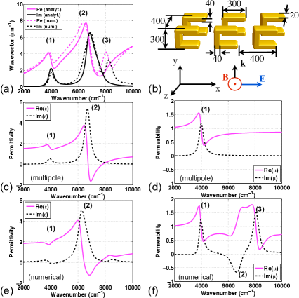
Figure 2: (a) Comparison of the dispersion relation - numerical model (dashed), analytical model (solid); (b) Single metamaterial layer (gold SRR) used for the numerical simulation (dimensions in nm); spectral dependence of effective permittivity (c) and effective permeability (d) from the multipole model; spectral dependence of effective permittivity (e) and effective permeability (f) from the numerical simulations.

The obtained linear wave equations describe the field propagation in an effective medium determined by its multipolar contributions. Thus the correlated wave vector $k(\omega)$, i.e. the dispersion relation, represents a self consistent solution and contains all physical information to describe light propagation in the respective metamaterial. This can be understood in complete analogy to the exact parameter retrieval which assumes also a homogeneous wave propagation inside a metamaterial slab. By neglecting the the nonlinear source terms $q_{\omega;2\omega,-\omega}$ and $q_{2\omega;\omega,\omega}$ in Eq.(10) we get the linear wave equation

$$\left[\frac{\partial^{2}}{\partial y^{2}}+\frac{\omega^{2}}{c^{2}}+\omega^{2}\mu_{0}p_{\omega}-\mu_{0}\left[\omega^{2}q_{\omega}-i\omega m_{\omega}\right]\frac{\partial}{\partial y}\right]$$

$$\times e^{ik(\omega)y}=0.$$ (13)

For plane waves their solution yields the linear dispersion relation

$$k^{2}(\omega) = \frac{\omega^{2}}{c^{2}}\left[1+\frac{p_{\omega}}{\epsilon_{0}}-ik(\omega)\left(\frac{q_{\omega}}{\epsilon_{0}}-i\frac{m_{\omega}}{\epsilon_{0}\omega}\right)\right].$$ (14)

Together with the multipole definitions [Eqs.(11)] this implicit equation becomes

$$k^{2}(\omega) = \frac{\omega^{2}}{c^{2}}[1+\frac{4\eta q\chi^{+}_{\omega}\cos(k(\omega)y_{0})}{\epsilon_{0}}$$ (15)

$$+ \frac{4y_{0}k(\omega)\eta q\chi^{-}_{\omega}\sin(k(\omega)y_{0})}{\epsilon_{0}}],$$

which has to be solved numerically. However in the subwavelength limit $y_{0}<\lambda$ the trigonometric functions can be expanded

$$\cos(k(\omega)y_{0}) \approx 1-\frac{k^{2}(\omega)y_{0}^{2}}{2},$$

$$\sin(k(\omega)y_{0}) \approx k(\omega)y_{0}.$$ (16)

Thus the linear dispersion relation and hence the effective refractive index may be explicitly written down as

$$k^{2}(\omega)=\frac{\omega^{2}}{c^{2}}n^{2}_{\text{eff}}(\omega)=\frac{\omega^{2}}{c^{2}}\frac{1+\frac{4\eta q}{\epsilon_{0}}\chi^{+}_{\omega}}{1+\frac{\omega^{2}}{c^{2}}\frac{2\eta q}{\epsilon_{0}}y_{0}^{2}\left[\chi^{+}_{\omega}-2\chi^{-}_{\omega}\right]}.$$ (17)

The remaining unknown parameters of the introduced formalism can be obtained by fitting this dispersion relation to the numerically calculated one for the present gold SRR geometry, shown in FIG.(2a) Rockstuhl et al. (2008). As a result the two first resonances [denoted by (1) and (2)], which are the fundamental magnetic (1) and the fundamental electric (2) mode, are nicely covered by our dispersion relation. It can be clearly seen that the next higher magnetic mode [resonance (3)] is not covered by the multipole description. This would require to consider a more complex carrier dynamic as it can be deduced from numerical simulations Rockstuhl et al. (2006). Moreover, the effective parameters ($\epsilon_{\mathrm{eff}},~{}\mu_{\mathrm{eff}}$) follow without any further fitting Petschulat et al. (2008) and show a good agreement in comparison with the corresponding numerically determined values FIG.(2c-f). In order to determine the effectice permittivity and permeability too we have to consider the constitutive relations Jackson (1975); Raab and Lange (2005), by which we introduce both quantities. We start with the electric permittivity

$$\textbf{D}(\textbf{r},t) = \epsilon_{0}\textbf{E}(\textbf{r},t)+\textbf{P}(\textbf{r},t)-\nabla\cdot\mathbf{\hat{Q}}(\textbf{r},t),$$

$$D_{x}(y,t) = \epsilon_{0}E_{x}(y,t)+P_{x}(y,t)-\frac{\partial}{\partial y}Q_{xy}(y,t),$$

$$D_{\omega} = \epsilon_{0}\left[1+\frac{p_{\omega}}{\epsilon_{0}}-ik(\omega)\frac{q_{\omega}}{\epsilon_{0}}\right]E_{\omega},$$

$$\epsilon_{\text{eff}}(\omega) \equiv 1+\frac{p_{\omega}}{\epsilon_{0}}-ik(\omega)\frac{q_{\omega}}{\epsilon_{0}}.$$ (18)

In complete analogy we derive the effective magnetic permeability and begin with

$$\textbf{H}(\textbf{r},t) = \frac{1}{\mu_{0}}\textbf{B}(\textbf{r},t)-\textbf{M},$$

$$H_{z}(y,t) = \frac{1}{\mu_{0}}B_{z}(y,t)-M_{z}(y,t),$$

$$H_{\omega} = \frac{1}{\mu_{0}}B_{\omega}-m_{\omega}E_{\omega}.$$ (19)

At this point it becomes evident that the effective magnetic response is merely evoked by the electric field Tretyakov (2003). This is a consequence of the underlying model, because the complete carrier dynamics is driven by the electric field only. Within the multipole expansion this carrier dynamics, i.e. the plasmonic eigemodes are transformed into multipole moments including the magnetic dipole moment. Thus, all moments, even the magnetic moment, are a mere consequence of the electric field interaction with microscopic carriers. We mention that this is occasionally erroneously interpreted, by an argumentation that the magnetic moment is induced by the magnetic field. Our approach shows that all effects, also magnetic ones, may be sufficiently well described by an electric field interaction only. Nevertheless, to define the magnetic permeability it is necessary to translate the electric field into a magnetic field which yields

$$E_{\omega} = -\frac{\omega}{k(\omega)}B_{\omega},$$

$$H_{\omega} = \frac{1}{\mu_{0}}\left[1+m_{\omega}\frac{\omega}{\mu_{0}k(\omega)}\right]B_{\omega},$$

$$\mu_{\text{eff}}(\omega) \equiv \frac{1}{1+m_{\omega}\frac{\omega}{\mu_{0}k(\omega)}}.$$ (20)

In contrast to the retrieval of the systems parameters we have fitted the disperison relation to the model, but in turn this can be performed equivalently for the effective material parameters $\epsilon_{\text{eff}}$ and $\mu_{\text{eff}}$, yielding the same physical information with respect to the required quantities.

IV Nonlinear optical Properties - Second Harmonic Generation

To study the nonlinear behavior induced by the fundamental modes of the present metaatom we resort to the linear dispersion relation and treat the nonlinearity as perturbation rather than solving Eqs.(10) exactly. As usual we rely on the slowly varying envelope approximation (SVEA) Butcher and Cotter (1990). Within this approximation the fast spatial oscillation $\exp[ik(\omega)y]$ is separated from a slowly varying amplitude $A(y)$, which contains all information about the generation and depletion of the fundamental ($E_{\omega}=A_{\omega}(y)\exp[ik(\omega)y]$) and the second harmonic ($E_{2\omega}=A_{2\omega}(y)\exp[ik(2\omega)y]$).

IV.1 Exact numerical solution

At first the solution to the wave equations incorporating the SVEA ansatz has been performed numerically. Therefore we simplify this system by introducing the following substitutions

$$\delta_{\omega} \equiv \frac{\omega^{2}}{c^{2}}+\omega^{2}\mu_{0}p_{\omega},$$

$$\beta_{\omega} \equiv \mu_{0}\left(\omega^{2}q_{\omega}-i\omega m_{\omega}\right),$$

$$\psi_{\omega;2\omega,-\omega} \equiv \omega^{2}\mu_{0}q_{\omega;2\omega,-\omega},$$

$$\psi_{2\omega;\omega,\omega} \equiv 4\omega^{2}\mu_{0}q_{2\omega;\omega,\omega}.$$ (21)

Now the eigenvalue equations take the following form

$$\left\{\frac{\partial^{2}}{\partial y^{2}}+\delta_{\omega}-\beta_{\omega}\frac{\partial}{\partial y}\right\}E_{\omega}e^{i(k(\omega)y} = -\psi_{\omega;2\omega,-\omega}\frac{\partial}{\partial y}\left[E_{\omega}^{\dagger}E_{2\omega}e^{i(k(2\omega)-k(\omega)^{\dagger})y}\right],$$

$$\left\{\frac{\partial^{2}}{\partial y^{2}}+\delta_{2\omega}-\beta_{2\omega}\frac{\partial}{\partial y}\right\}E_{2\omega}e^{i(k(2\omega)y} = -\psi_{2\omega;\omega,\omega}\frac{\partial}{\partial y}\left[E_{\omega}^{2}e^{i2k(\omega)y}\right].$$ (22)

The solution to these equations are two coupled nonlinear dispersion relations, one for the fundamental and one for the second harmonic wave, which depend on both fields. In order to avoid the solution of this involved system we treat the nonlinearity as a perturbation and resort to the linear dispersion relation. To study the effect of the nonlinear source terms we apply the slowly varying envelope approximation where the linear fields are weighted by a slowly varying amplitude functions $A(y)$. Replacing the constant amplitudes $E_{\omega,2\omega}$ by $A_{\omega,2\omega}(y)$ we obtain upon substitution and upon neglection of the second-order derivatives (SVEA)

$$\frac{\partial}{\partial y}A_{\omega}(y) = -\frac{\psi_{\omega;2\omega,-\omega}}{2ik(\omega)-\beta_{\omega}}\left(A_{2\omega}(y)\frac{\partial}{\partial y}A_{\omega}(y)^{\dagger}+A_{\omega}(y)^{\dagger}\frac{\partial}{\partial y}A_{2\omega}(y)+i(k(2\omega)-k^{\dagger}(\omega))A_{\omega}(y)^{\dagger}A_{2\omega}(y)\right)$$

$$\times e^{i(k(2\omega)-k(\omega)^{\dagger}-k(\omega))y},$$

$$\frac{\partial}{\partial y}A_{2\omega}(\omega) = -\frac{\psi_{2\omega;\omega,\omega}}{2ik(2\omega)-\beta_{2\omega}}\left(2A_{\omega}(y)\frac{\partial}{\partial y}A_{\omega}(y)+2ik(\omega)A_{\omega}^{2}(\omega)\right)e^{i(2k(\omega)-k(2\omega))y}.$$ (23)

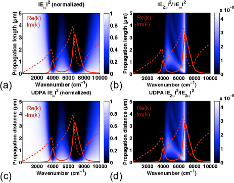
Figure 3: Evolution of normalized electric field intensity for the FF (a) and the SH (b) as a function of the wavenumber. The red lines indicate the real (dashed) and the imaginary part (solid) of the linear dispersion relation. (c), (d) The corresponding results for the un-depleted pump approximation (UDPA).

This final system has been solved numerically [FIG.(3)]. The FF wave evolution $E_{\omega}(y)$ is determined by the two eigenmode resonances (both indicated by the resonances in the red lined dispersion relation), where a strong damping is observed. For frequencies out of the spectral domain of these resonances the FF wave propagates without excessive losses, as expected. For the SH wave a strong contribution at the fundamental magnetic and electric resonance can be observed. In these calculations the SHG signal originating from the electric resonance around $\bar{\nu}=6400~{}\mathrm{cm}^{-1}$ seems to be much stronger than in the spectral vicinity of the magnetic resonance ($\bar{\nu}=4000~{}\mathrm{cm}^{-1}$). This originates from the strong damping of the SHG wave for the magnetic resonance (which propagates at $\bar{\nu}\approx 8000~{}\mathrm{cm}^{-1}$), because in this spectral domain an enhanced damping occurs due to the presence of the electric resonance. This changes dramatically for the SH wave induced by the electric mode, since at the SH frequency the imaginary part of $k(2\omega)$ is close to zero. Thus the second harmonic originating from the electric resonance propagates almost without damping.

IV.2 Un-depleted pump approximation

In order to double-check the results and to take the weak conversion efficiency into account the undepleted pump approximation (UDPA) has been applied Butcher and Cotter (1990). Within this approximation the fundamental wave (the pump) remains unaffected by the generated second harmonic wave. This can be expressed by setting $\psi_{\omega;2\omega,-\omega}$ in the first equation as well as the first derivative of $A_{\omega}(y)$ in the second equation to zero. This results in

$$\frac{\partial}{\partial y}A_{2\omega}(y) = \frac{-\psi_{2\omega;\omega,\omega}}{2ik(2\omega)-\beta_{2\omega}}2ik(\omega)A_{\omega}^{2}(y)e^{i(2k(\omega)-k(2\omega)y)},$$

$$A_{2\omega}(y) = \frac{\psi_{2\omega;\omega,\omega}}{2ik(2\omega)-\beta_{2\omega}}\frac{2k(\omega)}{2k(\omega)-k(2\omega)}A_{\omega}^{2}(y)$$ (24)

$$\times \left(1-e^{i(2k(\omega)-k(2\omega)y)}\right).$$

Comparing the numerically determined electric field for the fundamental and the second harmonic wave to those of the undepleted pump approximation [see FIG.(3)] one can clearly deduce that the UDPA describes the propagation for both waves almost exactly. Furthermore Eq.(IV.2) permits to calculate analytically the conversion efficiency from fundamental to second harmonic intensity, e.g. for a slab consisting of a single layer of SRR’s. It is important to note that for this purpose only parameters are required, that are fixed by comparison with the linear effective material response. In passing we comment that such a procedure; the determination of the nonlinear material properties based on the linear material parameters, is known as Miller’s delta a well established rule in nonlinear optics Miller (1964); Choy and Byer (1976).

V Summary

In summary, we have presented a self-consistent physical model that permits to describe the linear response of metaatom geometries by their intrinsic plasmonic eigenmodes. The occurring specific carrier dynamics have been mimicked by an auxiliary carrier alignment interacting with the incident radiation. The knowledge of these charge oscillations allows the application of the multipole expansion which provides the eigenvalue equation for electromagnetic waves propagating in such a composite metamaterial. Moreover we have shown that the specific convective carrier oscillations together with the quadrupole moment inherently introduce nonlinear material interactions. Considering the SHG process, our calculations show the expected enhanced signal both for the electric and the magnetic resonance and provide a microscopical and physical understanding of them. For further investigations it is important that the nonlinear response can be determined only from knowing the linear response, which is accessible by comparing the dispersion relation or any other effective material property to the introduced multipole model.
Financial support by the Federal Ministry of Education and Research as well as from the State of Thuringia within the Pro-Excellence program is acknowledged.

References

- Pollard et al. (2009) R. J. Pollard, A. Murphy, W. R. Hendren, P. R. Evans, R. Atkinson, G. A. Wurtz, A. V. Zayats, and V. A. Podolskiy, Phys. Rev. Lett. 102, 127405 (2009).
- Valentine et al. (2008) J. Valentine, S. Zhang, T. Zentgraf, E. Ulin-Avila, D. A. Genov, G. Bartal, and X. Zhang, Nature 455, 376 (2008).
- Pendry (2008) J. Pendry, Science 322, 71 (2008).
- Cai et al. (2007) W. Cai, U. K. Chettiar, A. V. Kildishev, and V. M. Shalaev, Nature Photon. 1, 224 (2007).
- Rockstuhl et al. (2006) C. Rockstuhl, F. Lederer, C. Etrich, T. Zentgraf, J. Kuhl, and H. Giessen, Opt. Express 14, 8827 (2006).
- Rockstuhl et al. (2007) C. Rockstuhl, T. Zentgraf, E. Pshenay-Severin, J. Petschulat, A. Chipouline, J. Kuhl, T. Pertsch, H. Giessen, and F. Lederer, Opt. Express 15, 8871 (2007).
- Esteban et al. (2008) R. Esteban, R. Vogelgesang, J. Dorfmüller, A. Dmitriev, C. Rockstuhl, and K. K. C Etrich, Nano Lett 8, 3155 (2008).
- Han et al. (2008) D. Han, Y. Lai, K. H. Fung, Z.-Q. Zhang, and C. T. Chan, Arxiv preprint arXiv:0812.2717v1 (2008).
- Sharma (2007) N. L. Sharma, Phys. Rev. Lett. 98, 217402 (2007).
- David J. Cho et al. (2008) F. W. David J. Cho, X. Zhang, and Y. R. Shen, Phys. Rev. B 78, 121101(R) (2008).
- D Shin (2000) Y. L. D Shin, A Chavez-Pirson, Opt. Lett. 15, 171 (2000).
- Guzatov et al. (2008) D. Guzatov, V. Klimov, and M. Pikhota, Arxiv preprint arXiv:0811.4070 (2008).
- Petschulat et al. (2008) J. Petschulat, C. Menzel, A. Chipouline, C. Rockstuhl, A. Tünnermann, F. Lederer, and T. Pertsch, Phys. Rev. A 78, 043811 (2008).
- Pustovit et al. (2002) V. Pustovit, J. Sotelo, and G. Niklasson, JOSA A 19, 513 (2002).
- Bloembergen (1965) N. Bloembergen, Nonlinear optics (Benjamin Press, New York, 1965).
- Pershan (1963) P. S. Pershan, Phys. Rev. 130, 919 (1963).
- Kujala et al. (2007) S. Kujala, B. K. Canfield, M. Kauranen, Y. Svirko, and J. Turunen, Phys. Rev. Lett. 98, 167403 (2007).
- Bethune (1981) D. Bethune, Opt. Lett. 6, 287 (1981).
- Bachelier et al. (2008) G. Bachelier, I. Russier-Antoine, E. Benichou, C. Jonin, and P.-F. Brevet, JOSA B 25, 955 (2008).
- Jayabalan et al. (2008) J. Jayabalan, Manoranjan, P. Singh, A. Banerjee, and K. C. Rustagi, Phys. Rev. B 77, 1 (2008).
- Kim et al. (2008) E. Kim, F. Wang, W. Wu, Z. Yu, and Y. R. Shen, Phys. Rev. B 78, 1 (2008).
- Maluckov et al. (2008) A. Maluckov, L. Hadzievski, N. Lazarides, and G. P. Tsironis, Phys. Rev. E 77, 1 (2008).
- Shadrivov et al. (2008a) I. V. Shadrivov, A. B. Kozyrev, D. W. V. D. Weide, and Y. S. Kivshar, Appl. Phys. Lett. 93, 161903 (2008a).
- Shadrivov et al. (2008b) I. Shadrivov, A. Kozyrev, D. van der Weide, and Y. Kivshar, Opt. Express 16, 20266 (2008b).
- Zharov et al. (2003) A. Zharov, I. Shadrivov, and Y. Kivshar, Phys. Rev. Lett. 91, 037401 (2003).
- Klein et al. (2006) M. W. Klein, C. Enkrich, M. Wegener, and S. Linden, Science 313, 502 (2006).
- Klein et al. (2007) M. W. Klein, M. Wegener, N. Feth, and S. Linden, Opt. Express 15, 5238 (2007).
- Feth et al. (2008) N. Feth, S. Linden, M. Klein, M. Decker, F. Niesler, Y. Zeng, W. Hoyer, J. Liu, S. Koch, J. Moloney, et al., Opt. Lett. 33, 1975 (2008).
- Zeng et al. (2009) Y. Zeng, W. Hoyer, J. Liu, S. W. Koch, and J. V. Moloney, Arxiv preprint arXiv:0807.3575v2 (2009).
- Butcher and Cotter (1990) P. Butcher and D. Cotter, The elements of nonlinear optics (Cambridge University Press, Cambridge, 1990).
- Rockstuhl et al. (2008) C. Rockstuhl, C. Menzel, T. Paul, T. Pertsch, and F. Lederer, Phys. Rev. B 78, 155102 (2008).
- Jackson (1975) J. D. Jackson, Classical Electrodynamics (Wiley, New York, 1975).
- Raab and Lange (2005) R. E. Raab and O. L. D. Lange, Multipole Theory in Electromagnetism (Clarendon, Oxford, 2005).
- Tretyakov (2003) S. Tretyakov, Analytical Modeling in Applied Electromagnetics (Artech House, Boston, 2003).
- Miller (1964) R. Miller, Appl. Phys. Lett. 5, 17 (1964).
- Choy and Byer (1976) M. Choy and R. Byer, Phys. Rev. B 14, 1693 (1976).