Drag reduction in pipe flow by optimal forcing

Abstract

In most settings, from international pipelines to home water supplies, the drag caused by turbulence raises pumping costs many times higher than if the flow were laminar. Drag reduction has therefore long been an aim of high priority. In order to achieve this end, any drag reduction method must modify the turbulent mean flow. Motivated by minimization of the input energy this requires, linearly optimal forcing functions are examined. It is shown that the forcing mode leading to the greatest response of the flow is always of $m=1$ azimuthal symmetry. Little evidence is seen of the second peak at large $m$ (wall modes) found in analogous optimal growth calculations, which may have implications for control strategies. The model’s prediction of large response of the large length-scale modes is verified in full direct numerical simulation of turbulence ($Re=5300$, $Re_{\tau}\approx 180$). Further, drag reduction of over 12% is found for finite amplitude forcing of the largest scale mode, $m=1$. Significantly, the forcing energy required is very small, being less than 2% of that by the through pressure, resulting in a net energy saving of over 10%.

Eddies in turbulent flow dramatically elevate the effective viscosity of the fluid, and thereby the friction drag at the wall. The ever increasing pressure for energy efficiency has heightened interest in turbulent drag reduction. Whilst strategies for drag reduction have been developed in principle, unfortunately few have yet been realised with a net energy saving.

In wall-bounded turbulent shear flows two distinct spatial scales become relevant at large Reynolds number: the outer scale $h$ (e.g the radius of the pipe, or the half-width of the channel) and the inner-scale $\nu/u_{\tau}$, which depends on the fluid kinematic viscosity $\nu$ and on the ‘wall’-velocity, $u_{\tau}=(\tau_{w}/\rho)^{1/2}$, based on the wall shear-stress $\tau_{w}$. One of many potential difficulties is that most of the proposed strategies are based on the control of near-wall structures, which both change with the Reynolds number and are extremely small at large Reynolds numbers. Turbulent skin friction is known to be closely associated with near-wall structures which scale on this inner scale Choi et al. (1994). Understandably, there have been many investigations to manipulate these near-wall vortical structures, for example, opposition controls Choi et al. (1994) and spanwise oscillation of entire wall Jung et al. (1999); Quadrio and Ricco (2004) for plane channel flow, and Choi and Graham (1997); Quadrio and Sibilla (2000) for pipe flow. These methods offer $\approx$7% net energy savings, although a large part of the energy budget may be required to modify the flow. Passive methods, requiring no external energetic input other than the driving pressure, are another promising route. Streamwise aligned riblets have been used to produce energy savings, also around 7%, much more cheaply than via active units Walsh (1990); Bechert and Bartenwerfer (1989). Unfortunately, each riblet must scale on the inner scale, and may require cleaning should the deposition of wax or dirt occur.

As an alternative route to the manipulation of individual near-wall structures, it has been suggested that many could be manipulated at once by means of large-scale control. The concept was proven in a nice study of the channel flow Schoppa and Hussain (1998) by imposing large streamwise vortices $\lambda^{+}\approx 400$. The spacing of near-wall structures is typically $\approx 100$ wall-units Kline et al. (1967). Drag reduction reaching $20$% was achieved, and while the effective work done to impose the vortices was not documented, their amplitude was only 6% of the centre-line speed. The feasibility of this strategy has been confirmed by an experimental investigation Iuso et al. (2002) in the flat plate boundary layer where large scale vortices were forced using vortex generators mounted on the wall. It was preliminarily shown that forcing at large spanwise scale ($\lambda^{+}\approx 1000$) is also effective in reducing the drag.

It is convenient that large-scale vortices can induce drag reduction, as it is known they can be efficiently forced efficiently in laminar flows Butler and Farrell (1992); Schmid and Henningson (2001). It has also been realised, via the study of optimal perturbations, that the emergence of large scale motions is important in turbulent flows del Álamo and Jiménez (2006); Pujals et al. (2009); Cossu et al. (2009); Hwang and Cossu (2009). Optimal perturbations consist of streamwise uniform vortices that optimally extract energy from the mean flow while inducing the growth of the streaks. As the large-scale optimal vortices scale on the outer scale, they are apt to implementation for control, as their shape is much more dependent on the domain geometry than on the Reynolds number. Further, the energy input necessary to obtain a desired amplitude of streak decreases when the Reynolds number is increased. In other words, the efficiency of the forcing of the large scale streaks increases with the Reynolds number.

The scope of the present investigation is twofold. First we compute the optimal coherent streamwise vortices and streaks for turbulent pipe flow, in particular to determine the associated optimal energy amplification. In doing so, large growth is demonstrated, and the optimal azimuthal and streamwise wavenumbers are identified. Second, we ascertain that forcing at finite amplitude can induce competitive drag reduction in the turbulent pipe. In our simulations the circumference corresponds to $\lambda^{+}_{m=1}\approx 1130$, and the forced rolls are significatly larger than the typical spacing of near-wall structures. As the structure of the forced large-scale motion does not depend strongly on the flow rate, there is promise that a method of forcing to produce drag reduction should be practical over large ranges of Reynolds numbers.

Consider the turbulent incompressible flow of a viscous fluid of kinematic viscosity $\nu$ in a circular pipe of radius $R$. The bulk velocity $U_{b}$ is assumed constant. Velocities are normalised by $2U_{b}$ and lengths by $R$. The Reynolds number is $Re=2\,U_{b}R/\nu$. Following the approach used in del Álamo and Jiménez (2006); Pujals et al. (2009); Cossu et al. (2009); Hwang and Cossu (2009), in order to compute optimal coherent perturbations, we consider small perturbations $p$ and $u$, to the pressure and turbulent mean flow $\mbox{\boldmath$U$}=U(y)\mbox{\boldmath$\hat{z}$}$, where $y=1-r$. The perturbations satisfy continuity and the linearised momentum equation:

$$\partial_{t}\mbox{\boldmath$u$}+u_{r}\,\partial_{r}U\mbox{\boldmath$\hat{z}$}+U\,\partial_{z}\mbox{\boldmath$u$}=-\mbox{\boldmath$\nabla$}p+\frac{1}{Re}\,\mbox{\boldmath$\nabla$}\cdot\left[\nu_{T}(y)\left(\nabla\mbox{\boldmath$u$}+\nabla\mbox{\boldmath$u$}^{T}\right)\right]+\mbox{\boldmath$f$},$$ (1)

where the total total normalised effective viscosity is $\nu_{T}(y)=1+E(y)$ with the $E(y)$ being the eddy viscosity. We use for $E(y)$ an expression originally suggested for pipe flow by Cess Cess (1958), later used for channel flows by Reynolds and Tiederman Reynolds and Tiederman (1967):

$$E(y) = \frac{1}{2}{\Big{\{}}1+\frac{\kappa^{2}\hat{R}^{2}\hat{B}}{9}[2y-y^{2}]^{2}(3-4y+2y^{2})^{2}\times\left[1-\exp\left(\frac{-y\hat{R}\sqrt{\hat{B}}}{A^{+}}\right)\right]{\Big{\}}}^{\frac{1}{2}}-\frac{1}{2}\,.$$ (2)

with $\hat{R}=Re\,/\,2$,  $\hat{B}=2\,B$ and the fitting parameters $A^{+}=27$ and $\kappa=0.42$ chosen to better match the observations, more recently studied in McKeon et al. (2005). The mean streamwise velocity $U(y)$ in equilibrium with this eddy viscosity is easily retrieved from the mean averaged momentum equation equation

$$0=-\partial_{z}P+\frac{1}{Re}\left(\frac{1}{r}+\partial_{r}\right)(\nu_{T}\partial_{r}U),\qquad B=-\partial_{z}P.$$ (3)

The symmetry of the base flow allows one to consider separately perturbations of the form $\mbox{\boldmath$u$}(r,\theta,z;t)=\hat{\mbox{\boldmath$u$}}(r,m,\alpha;t)\,{\rm e}^{{\rm i}(\alpha z+m\theta)}$, where $\alpha$ and $m$ are the streamwise and azimuthal wavenumbers respectively. The eigenvalues and eigenvectors are found directly from the linearised primitive variable system with explicit solenoidal condition . For all calculations considered $U(y)$ is found to be linearly stable, in accordance with similar results obtained in the plane channel and boundary layer flows Reynolds and Tiederman (1967); del Álamo and Jiménez (2006); Cossu et al. (2009); Pujals et al. (2009); Hwang and Cossu (2009).

The optimal response to forcing is calculated using methods described in Schmid (2007). For a harmonic forcing of the form $\mbox{\boldmath$\hat{f}$}(r,m,\alpha;t)=\mbox{\boldmath$\tilde{f}$}(r,m,\alpha)\,{\mathrm{e}}^{{\mathrm{i}}\,\Omega_{f}t}$ and response $\mbox{\boldmath$\hat{u}$}(r,m,\alpha;t)=\mbox{\boldmath$\tilde{u}$}(r,m,\alpha)\,{\mathrm{e}}^{{\mathrm{i}}\,\Omega_{f}t}$ the optimal response is given by

$$R(\alpha,m;\Omega_{f})=\max_{\mbox{\boldmath$\tilde{f}$}}\,\frac{||\mbox{\boldmath$\tilde{u}$}||}{||\mbox{\boldmath$\tilde{f}$}||}\,,\quad R_{\mathrm{max}}(\alpha,m)=\max_{\Omega_{f}}R(\Omega_{f}).$$ (4)

Figure 1 shows our calculations for the optimal response to forcing for several $Re$ . The optimal response $R_{\mathrm{max}}$ generally increases with increasing $Re$. As the spanwise length-scale is decreased ($m$ increased) the response rapidly decreases. The largest possible response occurs for the mode $m=1$.

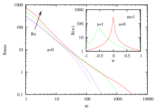
Figure 1: Response $R_{\mathrm{max}}(\alpha=0,m)$ to forcing, $Re=5300$, $10^{4}$, $10^{5}$, $10^{6}$, the arrow indicating increasing $Re$. Inset: $Re=5300$, $m=1$, response to forcing of frequency $\Omega_{f}$. The turbulent flow is most responsive to axially-independent steady forcing on the largest scale.

Huge response to forcing of large scale modes is possible. The relative difficulty of forcing motion on small scales, on the other hand, implies that considerable effort is required to locally manipulate structures in the neighbourhood of the wall.

The analysis above is linear and uses the eddy viscosity assumption. A first step towards application is to verify that large responses are obtained in fully nonlinear turbulent numerical simulation. The pipe flow code described in Willis and Kerswell (2009) has been used for full simulation of turbulence subject to the optimal forcing $\tilde{f}$. The numerical method uses a Fourier decomposition in $\theta$ and $z$ and finite differences in $r$ . For the following calculations the computational domain is of length $L=15R$, chosen to include the very large-scale motions reported in Kim and Adrian (1999) for $L$ up to $14$. We choose to perform the simulations enforcing a fixed flux, consistent with previous analyses Schoppa and Hussain (1998); Willis and Kerswell (2009).

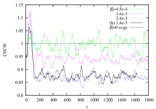
Figure 2: Relative drag for several $||\mbox{\boldmath$\tilde{f}$}||$ at $Re=5300$. The straight horizontal line is the unforced average. The solid line is a higher resolution check for the best case.

Figure 2 shows time series for the skin-friction coefficient, $C_{f}=2(u_{\tau}/U_{b})^{2}$, for three levels of forcing of the $m=1$ mode at $Re=5300$. The horizontal line is the time average $C_{f}$ for zero forcing. The solid line for a higher resolution calculation verifies no loss of the observed drag reduction for the case shown.

The response to forcing in simulations is measured by $R^{\prime}=||\mbox{\boldmath$\bar{u}$}||\,/\,||\mbox{\boldmath$\tilde{f}$}||$, where the averaged response field is $\bar{\mbox{\boldmath$u$}}(r,\theta)=\langle\mbox{\boldmath$u$}\rangle_{z,t}-U(r)\,\hat{\mbox{\boldmath$z$}}$ and $U(r)=\langle\mbox{\boldmath$u$}\rangle_{\theta,z,t}$ is the mean flow in the absence of forcing. The norm used here is $||\mbox{\boldmath$a$}||^{2}=\frac{1}{L}\int\mbox{\boldmath$a$}\cdot\mbox{\boldmath$a$}\,\mathrm{d}V$ and $\langle\,\cdot\,\rangle_{s}$ indicates averaging over the subscripted variables. Time averages are taken over $1400\,R/(2U_{b})$ time units. Measures of streak and roll components of the flow are $A_{z}=\frac{1}{2}(\max\bar{u}_{z}-\min\bar{u}_{z})$ and $A_{h}=\max|(\bar{u}_{r},\bar{u}_{\theta},0)|$.

In table 1 it is seen that the response to forcing may indeed be large, in agreement with the model. The prediction from the linear model is $R_{\mathrm{max}}=276$ for $m=1$, and there remains a factor $2$ difference, however, with the simulations for the two smallest $||\mbox{\boldmath$\tilde{f}$}||$. As the time-averaged mean flow for the unforced case, obtained from numerical simulation, is close to that given by (2) and (3), the difference must originate from the isotropic eddy viscosity assumption. While at first both $A_{z}$ and $A_{h}$ increase linearly with $||\mbox{\boldmath$\tilde{f}$}||$, streaks saturate near 19% of the centre-line speed. Streak saturation occurs when the roll amplitude is approximately 7% of the centre-line speed, and coincides with when the maximum drag reduction is achieved.

$||\mbox{\boldmath$f$}||$	$R^{\prime}$	$P$	$W$	$\mathrm{DR}$	$E_{\mathrm{net}}$	$A_{h}/U_{cl}$	$A_{z}/U_{cl}$
($m=1$)
1.4e-4	146.0	3.680e-3	1.03e-6	0.2	0.2	0.0091	0.0372
4.5e-4	138.0	3.675e-3	1.10e-5	0.4	0.1	0.0217	0.1088
7.7e-4	109.7	3.456e-3	3.29e-5	6.3	5.4	0.0444	0.1620
1.0e-3	90.3	3.230e-3	5.02e-5	12.4	11.1	0.0540	0.1847
1.2e-3	77.1	3.222e-3	6.53e-5	12.6	10.9	0.0618	0.1884
1.4e-3	63.3	3.218e-3	8.77e-5	12.8	10.4	0.0740	0.1890
2.0e-3	41.4	3.356e-3	1.57e-4	9.0	4.8	0.1049	0.1899
2.4e-3	33.1	3.470e-3	2.24e-4	5.9	-0.1	0.1308	0.1946
4.5e-3	16.3	3.990e-3	5.58e-4	-8.1	-23.3	0.1886	0.1953
($m=2$)
7.7e-4	118.0	3.358e-3	2.40e-5	9.0	8.3	0.0355	0.1605
1.4e-3	102.4	3.306e-3	7.81e-5	10.4	8.3	0.0699	0.2608
2.4e-3	62.7	3.660e-3	1.75e-4	0.8	-4.0	0.0910	0.2691
($m=4$)
4.5e-4	130.6	3.557e-3	9.66e-6	3.6	3.3	0.0224	0.1133
7.7e-4	137.9	3.540e-3	2.87e-5	4.0	3.2	0.0461	0.2208
1.4e-3	92.0	3.958e-3	6.79e-5	-7.3	-9.1	0.0653	0.2638
($m=12$)
7.7e-5	46.4	3.702e-3	8.64e-8	-0.3	-0.3	0.0012	0.0072
2.4e-4	46.3	3.714e-3	7.07e-7	-0.7	-0.7	0.0034	0.0183
7.7e-4	24.6	3.951e-3	6.35e-6	-7.1	-7.3	0.0099	0.0494

Table 1: Time averaged statistics for turbulent pipe flow subject to forcing. $P^{0}=$3.689e-3, $U_{cl}=U(r=0)=0.6556$. Largest drag reduction and net energy reduction in bold.

Also in table 1 is the percentage drag reduction $\mathrm{DR}=(100/C_{f}^{0})(C_{f}^{0}-C_{f})$, where superscripts $0$ indicate the unforced case. The power to drive the flow per unit length is $P=\frac{\pi}{8}C_{f}$ in units $\rho\,(2U_{b})^{3}\,R$. The relative change in $C_{f}$ for increased forcing is seen in figure 3. The drag reduction is up to $12.8$% and the greatest net energy saving up to $11.1$%, where $E_{\mathrm{net}}=(100/P^{0})[P^{0}-(P+W)]$. For the greatest $E_{\mathrm{net}}$, the power consumption by forcing, $W=\frac{1}{L}\int\mbox{\boldmath$u$}\cdot\mbox{\boldmath$\tilde{f}$}\,\mathrm{d}V$, is only $1.4$% of the power required to maintain the flux of the unforced flow, $P^{0}$, or $1.6$% of that to drive the resulting flow.

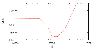
Figure 3: Effect of large-scale forcing, $m=1$, on the skin friction, $C_{f}$.

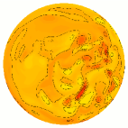
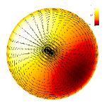
(a)	(b)	(c)
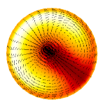
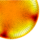
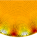
(d)	(e)	(f)

Figure 4: (a) Snapshot of axial vorticity with no forcing; (b) Snapshot on same scale as (a) for $||f||=$1.4e-3. (c) Arrows of the optimal forcing and contours of the optimal response; (d)-(f) Time averaged velocity for $||f||=$1.4e-3, 7.7e-4, 2.4e-4 for $m=1,4,12$ respectively, relative to $U(r)$ without forcing.

The effect of forcing on the flow is shown in figure 4. Small scale axial vortices are weakened throughout the domain, and are almost suppressed in one half. Being largely responsible for the turbulent skin friction Kravchenko et al. (1993), this indicates that near-wall turbulent production is suppressed by forcing large-scale outer motions, consistent with Schoppa and Hussain (1998). The large scale forcing structure is reproduced well in the roll structure of the time averaged flow. The broad slow streak, however, is clearly much narrower in the nonlinear response. This narrower slow streak means that several may be packed into the domain (e.g. $m=2,4$) before they affect each other ($m=12$). The case $m=12$ corresponds to the natural mean spacing of near wall structures $\lambda^{+}\approx 100$. For this case the response $R^{\prime}$ is significantly reduced, and drag only increases as the forcing is increased.

In summary, the model successfully predicts the large response to forcing observed in full simulation of turbulence. The largest response to forcing occurs for large-scale modes, which may have implications for control. Drag reduction of over 12% has been shown in full simulations when forcing the large-scale mode. Significantly, this was shown to be possible using very small input energy, being less than 2% of the energy used to drive the flow.

Several of the alternative methods described above predict much larger drag reduction, but at much greater energetic expense. This is possibly linked to the small response to forcing of near-wall vortices. The net energy saving is similar to that here, but relies on both the large drag reduction being realised at the same time as efficient actuation. For useful implementation of the method proposed in this study, the induction of rolls need not be efficient. For example, efficiency of 50%, still using only 4% of the driving energy, might be acceptable. Note also that the response is expected to increase with increasing $Re$, thereby reducing this cost. In practise, induction of large scale rolls is possible via passive actuators Fransson et al. (2004, 2006) or active jets Iuso et al. (2002). Although neither would reproduce the precise details of forcing used here, linear optimals are known to be robust to perturbations of the system, and responses close to those seen here can be expected. Slightly different responses, however, may also be beneficial — whilst the forcing in this numerical experiment is optimal for modifying the flow, it was not chosen to be optimal for drag reduction in the nonlinear régime. Thus there is scope for further enhancement.

References

- Choi et al. (1994) H. Choi, P. Moin, and J. Kim, J. Fluid Mech. 262, 75 (1994).
- Jung et al. (1999) W. J. Jung, N. Managiavacchi, and R. Akhavan, Phys. Fluids A 4, 1605 (1999).
- Quadrio and Ricco (2004) M. Quadrio and P. Ricco, J. Fluid Mech. 521, 251 (2004).
- Choi and Graham (1997) K.-S. Choi and M. Graham, Phys. Fluids 10, 7 (1997).
- Quadrio and Sibilla (2000) M. Quadrio and S. Sibilla, J. Fluid Mech. 424, 217 (2000).
- Walsh (1990) M. J. Walsh, Tech. Rep. (1990).
- Bechert and Bartenwerfer (1989) D. W. Bechert and M. Bartenwerfer, J. Fluid Mech. 205, 105 (1989).
- Schoppa and Hussain (1998) S. Schoppa and F. Hussain, Phys. Fluids 10, 1049 (1998).
- Kline et al. (1967) S. J. Kline, W. C. Reynolds, F. A. Schraub, and P. W. Runstadler, J. Fluid Mech. 30, 741 (1967).
- Iuso et al. (2002) G. Iuso, M. Onorato, P. G. Spazzini, and G. M. di Cicca, J. Fluid Mech. 473, 23 (2002).
- Butler and Farrell (1992) K. M. Butler and B. F. Farrell, Phys. Fluids A 4, 1637 (1992).
- Schmid and Henningson (2001) P. J. Schmid and D. S. Henningson, Stability and Transition in Shear Flows (Springer, New York, 2001).
- del Álamo and Jiménez (2006) J. C. del Álamo and J. Jiménez, J. Fluid Mech. 559, 205 (2006).
- Pujals et al. (2009) G. Pujals, M. García-Villalba, C. Cossu, and S. Depardon, Phys. Fluids (2009), in press.
- Cossu et al. (2009) C. Cossu, G. Pujals, and S. Depardon, J. Fluid Mech. 619, 79 (2009).
- Hwang and Cossu (2009) Y. Hwang and C. Cossu, in Sixth Symp. on Turbulence and Shear Flow Phenomena (Seoul Nat. University, Seoul Korea, 2009).
- Cess (1958) R. D. Cess, Westinghouse Research Rep. pp. no. 8–0529–R24 (1958).
- Reynolds and Tiederman (1967) W. C. Reynolds and W. G. Tiederman, J. Fluid Mech. 27, 253 (1967).
- McKeon et al. (2005) B. J. McKeon, M. V. Zagarola, and A. J. Smits, J. Fluid Mech. 538, 429 (2005).
- Schmid (2007) P. J. Schmid, Annu. Rev. Fluid Mech. 39, 129 (2007).
- Willis and Kerswell (2009) A. P. Willis and R. R. Kerswell, J. Fluid Mech. 619, 213 (2009).
- Kim and Adrian (1999) K. C. Kim and R. J. Adrian, Phys. Fluids 11, 417 (1999).
- Kravchenko et al. (1993) A. G. Kravchenko, H. Choi, and P. Moin, Phys. Fluids A 5, 3307 (1993).
- Fransson et al. (2004) J. Fransson, L. Brandt, A. Talamelli, and C. Cossu, Phys. Fluids 16, 3627 (2004).
- Fransson et al. (2006) J. Fransson, A. Talamelli, L. Brandt, and C. Cossu, Phys. Rev. Lett. 96, 064501 (2006).