Drifting instabilities of cavity solitons in vertical cavity surface-emitting lasers
with frequency selective feedback

Abstract

In this paper we study the formation and dynamics of self-propelled cavity solitons (CSs) in a model for vertical cavity surface-emitting lasers (VCSELs) subjected to external frequency selective feedback (FSF), and build their bifurcation diagram for the case where carrier dynamics is eliminated. For low pump currents, we find that they emerge from the modulational instability point of the trivial solution, where traveling waves with a critical wavenumber are formed. For large currents, the branch of self-propelled solitons merges with the branch of resting solitons via a pitchfork bifurcation. We also show that a feedback phase variation of $\pm 2\pi$ can transform a CS (whether resting or moving) into a different one associated to an adjacent longitudinal external cavity mode. Finally, we investigate the influence of the carrier dynamics, relevant for VCSELs. We find and analyze qualitative changes in the stability properties of resting CSs when increasing the carrier relaxation time. In addition to a drifting instability of resting CSs, a new kind of instability appears for certain ranges of carrier lifetime, leading to a swinging motion of the CS center position. Furthermore, for carrier relaxation times typical of VCSELs the system can display multistability of CSs.

Keywords: Moving soliton, resting soliton, swinging instability, localized traveling wave, feedback, VCSEL.

I Introduction

In recent years, there has been significant progress in the experimental Tanguy2006 ; TanguyPRL and theoretical Paulau2007 ; Paulau2008 study of self-localized states in vertical cavity surface-emitting lasers (VCSELs) subject to frequency selective external optical feedback (FSF). These systems are attractive from an experimental point of view because they can be implemented with basically off-the-shelf optical components, and they do not require an optical holding beam to support self-localized solutions, also known in this context as cavity solitons (CSs). These systems are known as Cavity Soliton Lasers, because for certain parameter regions laser emission takes place only in localized structures. An important property of this system is its invariance under phase transformations. Hence each CS is a member of a continuous family of phase-equivalent localized structures. Further, for the same parameters there may be several families of CSs with different frequencies. In contrast, localized structures in driven-cavity systems are phase- and frequency-locked to the holding beam.

There are many possible applications of CSs funfacs , but we will emphasize here only the most relevant one for the contents of this article, namely an optical delay line or shift register. This element is essential in communication systems for delaying pulses when routing several sequences of bits. This function was proposed to be implemented on the basis of spatially drifting CSs Pedaci2008 , where the drift of CSs was caused by a gradient of the system parameters. Thus, one can inject a sequence of pulses at one transverse position, and read out a copy of this sequence at another position at some later time (delay time of the shift register).

In contrast with gradient-induced CS motion, the possibility of self-motion was shown in a holding beam system Scroggie02 with thermal effects. Spontaneous motion of vortices in lasers and laser amplifiers with saturable absorption has been also studied in Rosanov . In a previous work Paulau2008 we have shown the existence of 2D self-propelled CSs in a VCSEL with FSF, even without thermal effects. This is an alternative mechanism to induce motion in delay lines. Since no parameter gradient has to be imposed and controlled, there is, in principle, no limit to the drift distance, and hence delay time of the shift register. Since CSs moving in the transverse direction can be reflected by the boundaries of the device PratiUnp the delay line can be folded, enabling longer paths for a given VCSEL aperture, and therefore improving the delay-bandwidth product.

In this article we analyze in detail the bifurcation diagram of self-moving solitons elucidating the conditions for the appearance of motion in the 1D case. In comparison with Paulau2008 here we address the role of the feedback phase, which plays an important role in determining the longitudinal-mode frequency of the CS. For a given feedback phase several CS solutions with different frequencies (associated to adjacent external cavity modes) are found to coexist. For each solution, sweeping the feedback phase allows to change continously the frequency of the CS. Applying a $2\pi$ sweep in the feedback phase shows a smooth transition from one CS solution branch to the adjacent one. The number of coexisting solutions increases with the delay time. We also investigate the role of the carrier dynamics, which was neglected in Paulau2008 , and analyze its influence on the stability of CSs. In particular we show the existence of a swinging instability in which the position of the CS maximum starts to perform growing oscillations near the initial position.

The paper is organized as follows: In Section II we discuss the system and the models considered. In Section III we describe the properties of self-propelled CSs and formulate the equations for their semianalytical calculation using a Newton method. In this section we present also the bifurcation diagrams of moving and resting solitons explaining their connection with the stability properties of the nonlasing background solution and discussing the relation between the 1D and the 2D problems. In section IV we study the possibilities of controlling the solitonic states by varying the feedback phase and show the co-existence of multiple states, both moving and resting. In Section V we study the influence of the carrier dynamics, leading to the swinging instability and to the stabilization of resting solitons. Finally, in Section VI we give some concluding remarks.

II System and Model

Following Tanguy2006 ; TanguyPRL ; Paulau2007 ; Paulau2008 , we consider the set-up sketched in Fig. 1), where light is fed back to the VCSEL after being filtered in frequency. The polarizer allows feedback only for the linearly polarized field component that is dominant in the solitary laser, so that the field can be treated as a scalar.

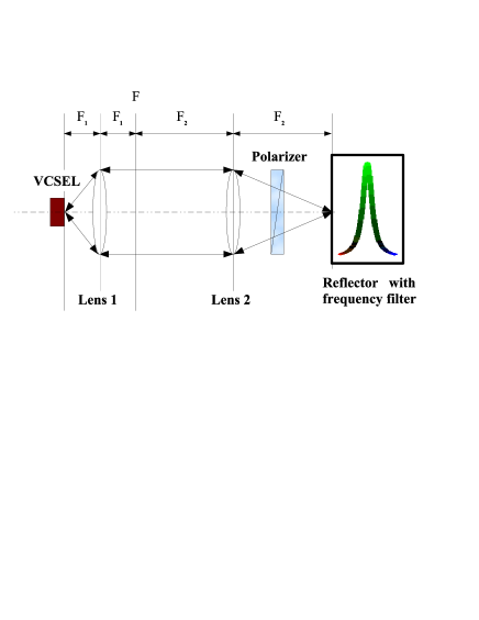
Figure 1: (Color online). Scheme of the system. $F_{1}$ and $F_{2}$ are the focal lengths of the first and second lenses respectively.

The dynamics of the complex envelope of the electrical field $E(x,t)$, the filtered feedback field $F(x,t)$ and the carrier number $N(x,t)$ can be described by

$$\left\{\begin{array}[]{l}\frac{\partial E}{\partial t}=\kappa(1+i\alpha)(N-1)E-i\Delta_{\perp}E+F+i\omega_{s}E,\\ \\ \frac{dF}{dt}=-\lambda F+\sigma e^{i\phi}\lambda E(t-\tau),\\ \\ \frac{dN}{dt}=\gamma\mu-\gamma N(1+|E|^{2}),\\ \end{array}\right.$$ (1)

where $\kappa$ is the decay rate of the field in the cavity; $\alpha$ is the linewidth enhancement factor describing phase-amplitude coupling; $\mu$ is the pump current normalized to be $1$ at the threshold of the solitary laser; $\Delta_{\perp}=\frac{\partial^{2}}{\partial x^{2}}$ describes diffraction and $\gamma=\frac{1}{T_{1}}$ is the carrier relaxation rate. The filter is considered to have a Lorentzian frequency response Jorge ; Yousefi99 ; Fisher2000 , and its central frequency is taken as referenceHence $\omega_{s}$ the frequency of the axial mode of the solitary laser at threshold ($N=1$). The other filter parameters are $\sigma$, the feedback strength, $\phi$ the feedback phase, $\tau$ the delay time in the feedback loop, and $\lambda$ the filter bandwidth.

Eliminating the carriers adiabatically model (1) reduces to

$$\left\{\begin{array}[]{l}\frac{\partial E}{\partial t}=-\kappa(1+i\alpha)E+\kappa(1+i\alpha)\frac{\mu E}{1+|E|^{2}}\\ \qquad\qquad\qquad\qquad-i\Delta_{\perp}E+F+i\omega_{s}E,\\ \\ \frac{dF}{dt}=-\lambda F+\sigma e^{i\phi}\lambda E(t-\tau),\\ \end{array}\right.$$ (2)

For a fixed feedback phase $\phi=0$ this was the model considered in Paulau2008 . We will use this simplified model in Sect. III to determine the bifurcation diagrams of moving and resting solitons as well as in Sect. IV to discuss the role of the feedback phase. While the simplified model allows for easier calculation, the typical relaxation times of the system are in fact $\kappa^{-1}\approx 0.01$ ns, $\lambda^{-1}\approx 0.2$ ns and $T_{1}\approx 1ns$ (throughout this paper time is measured in nanoseconds). Since the carrier density is the slowest variable, adiabatic elimination of the carriers is not fully justified. Nevertheless, as discussed in Sect. V where we address the influence of the carrier dynamics by considering the full model (1), the reduced model correctly predicts the existence of moving and resting stable CSs, albeit with slight changes in the parameter regions where they are observed.

III Resting and moving cavity solitons

We consider in this section the simplified model (2) for feedback phase $\phi=0$, as in Paulau2008 . Fig. 2 shows the marginal stability curves for the trivial solution $E=0$. This solution is stable for small pump values (below line D in the figure). At $\mu=\mu_{D}=1-\sigma/\kappa=0.4$ it becomes unstable to perturbations with the frequency of the filter maximum and with a finite transverse wavenumber. For values of the pump between lines D and B the formation of a complex spatiotemporal regime is observed. For pump values in between line B and the thick line at $\mu\approx 1$ the trivial solution is stable again. In this region, which we will call gap-region, we observe the spontaneous formation of self-localized states, both resting CSs and self-propelled CSs Paulau2008 . In the 1D case, we observe the formation of self-propelled CSs for almost all the values of the pump in the gap-region whereas in the 2D case this region splits in 3 subregions: a) close to B, where moving 2D CSs are excited, b) intermediate values, where resting 2D CSs are observed, and, c) values closer to 1, where no solitons can be excited Paulau2008 .

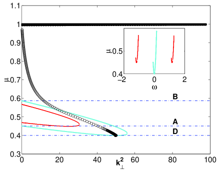
Figure 2: (Color online). Marginal stability curves of the nonlasing state in the VCSEL with external feedback. The inset shows the frequencies of the modes that become unstable between lines D and B in the main figure. The gray (cyan) curve corresponds to the boundary of excitation of external cavity modes with frequencies close to $\omega=0$ (the filter maximum). The line A corresponds to value of the pump at which the marginal instability curve gray (cyan) intersects the axis $k^{2}_{\perp}=0$. The thin dark (red) curve corresponds to the boundary of excitation of the two modes at either side of the dominant mode with frequencies $\omega\approx\pm\frac{2\pi}{\tau}\approx\pm 1.25$ (the boundary is practically the same for both modes for the parameters considered here). The thick black line corresponds to the excitation of modes with frequencies close to those of the solitary laser. The circles represent the square of the wavenumber of the far-field maximum for self-propelled 1D CSs. Stable localized solutions can exist in the region between the line B and the thick black line, in which the trivial solution is stable. Parameters: $\phi=0$, $\sigma=60$, $\alpha=5$, $\lambda=2.71$, $\tau=5$, $\omega_{s}=250$, $\kappa=100$.

The system is invariant under translational and global phase transformations, and thus the operations $E(x)\rightarrow E(x+x_{0})$ and $E(x)\rightarrow E(x)e^{i\psi_{0}}$ transform solutions in solutions. So there is a whole family of CSs which have the same distribution of the far field absolute value $|E(k)|$. The members of the family are identified by two continuous parameters, their location and global phase. Moving solutions break the left-right symmetry of the system so that two equivalent families of self-propelled CSs exist, one with a positive $k_{max}$ moving to the left and its specular image with negative $k_{max}$ and moving to the right.

The spatial distribution of a self-propelled 1D CS for $\mu=0.65$ is shown in Fig. 3. The near field is characterized by an exponential spatial localization. The far field shows a typical cascade of energy from small to large wavenumbers due to nonlinearity. The far field is centered off-axis (at $k_{max}=-2.54$ in Fig. 3) and is asymmetric: we note that the part of the far field to the right of the maximum is smoother than the left part. Self-propelled CSs move at a constant velocity, which is proportional to $-k_{max}$.

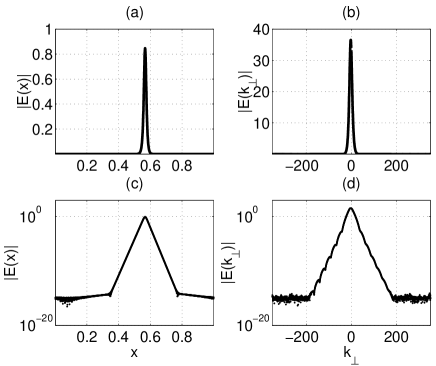
Figure 3: Shape of moving 1D CSs: (a) Near field, (b) far field, (c) near field in semilogarithmic scale, and (d) far field in semilogarithmic scale. Parameters are the same as in Fig. 2 and $\mu=0.65$.

The residual level at $\thicksim 10^{-16}$, both in the near and far fields, is indicative of the numerical precision. The spatial profile of the soliton shown in Fig. 3 has been obtained from numerical integration of Eq. (2) where the initial condition breaks the left-right degeneracy. As for the numerical integration, we should note that accurate results are difficult to obtain using usual finite difference methods, because large $k_{\perp}$ transverse wave vectors lead to the presence of very high frequencies, and hence they require very small temporal steps. For the numerical integration we have used the two-step pseudo-spectral method described in the appendix of Montagne2007 , where in Fourier space the linear part of the equations is handled analytically, thus avoiding the problem with the high frequencies associated to high wavenumbers due to diffraction. Nonlinear terms are evaluated in real space. The pseudo-spectral method can be easily adapted to equations with delay such as the ones considered here. We have taken the temporal stepsize much smaller than all the characteristic times of the system and we have verified that the selected stepsize allows to reproduce correctly the threshold of the background instability predicted by the linear stability analysis, and the threshold of the drifting instability obtained by the Newton method described below.

One of the main objectives of this work is, however, to compute the whole branch of self-propelled states, including the region where they are unstable, hence we need to implement a Newton method, similar to what was done for resting 2D solitons in Paulau2008 , for moving solutions. We will seek solutions of the form:

$$\left\{\begin{array}[]{l}E(x,t)=E_{o}(x+vt)e^{i\omega t},\\ \\ F(x,t)=F_{o}(x+vt)e^{i\omega t},\\ \end{array}\right.$$ (3)

Substituting (3) into (2) we have the following equations:

$$\left\{\begin{array}[]{l}-\frac{\partial E_{0}}{\partial x^{\prime}}v+(-\kappa(1+i\alpha)+i\omega_{s}-i\omega)E_{0}+\\ \qquad\qquad\qquad+\kappa(1+i\alpha)\mu\frac{E_{0}}{1+|E_{0}|^{2}}+i\frac{\partial^{2}E_{0}}{\partial x^{\prime 2}}+F_{0}=0,\\ \\ -\frac{\partial F_{0}}{\partial x^{\prime}}v-i\omega F_{0}-\lambda F_{0}+\sigma e^{i\phi}\lambda E_{0}(x^{\prime}-v\tau)e^{-i\omega\tau}=0,\\ \end{array}\right.$$ (4)

where $x^{\prime}=x+vt$ is the spatial coordinate in the moving reference frame. In Fourier space

$$F_{0}(k^{\prime})=\mathcal{F}(F_{0}(x^{\prime})),$$ (5)

$$E_{0}(k^{\prime})=\mathcal{F}(E_{0}(x^{\prime})),$$ (6)

$$\mathcal{F}(E_{0}(x^{\prime}-v\tau))=e^{ik^{\prime}v\tau}E_{0}(k^{\prime}),$$ (7)

the set of differential equations (4) is transformed into a set of algebraic equations. The second equation is linear and can be solved directly

$$F_{0}(k^{\prime})=\frac{\sigma e^{i\phi}\lambda e^{i(k^{\prime}v-\omega)\tau}}{\lambda+i(\omega+k^{\prime}v)}E_{0}(k^{\prime}),$$ (8)

leading to a single equation for the field $E_{0}$:

$$AE_{0}(k^{\prime})+B\mathcal{F}\left(\frac{\mathcal{F}^{-1}(E_{0}(k^{\prime}))}{1+|\mathcal{F}^{-1}(E_{0}(k^{\prime}))|^{2}}\right)=0,$$ (9)

where

$$A = -\kappa(1+i\alpha)+i(\omega_{s}-\omega-k^{\prime}v-k^{\prime 2})$$ (11)

$$+\frac{\sigma e^{i\phi}\lambda e^{i(k^{\prime}v-\omega)\tau}}{\lambda+i(\omega+k^{\prime}v)},$$

$$B = \kappa(1+i\alpha)\mu.$$ (12)

Equation (9) is analogous to the Eq. (3) of Paulau2008 for stationary solutions, while it also supports more complex solutions, like self-propelled CSs. In practice Eq. (9) is solved numerically by discretizing $k^{\prime}$ in $n$ values which leads to a set of $2n$ coupled equations. There are $2n+2$ unknowns [$E_{0}(k^{\prime}_{i})$ ($i=1,...n$), $v$ and $\omega$] and two constraints associated to the translational and global phase invariance. This set can be solved using a Newton method starting from an initial guess prepared by direct integration of (2). At each Newton iteration, imposing that in the moving frame the location of the CS does not change allows for the determination of $v$. Similarly imposing that the global phase does not change allows for the determination of $\omega$. Equivalent solutions can be obtained by applying a translation or a global phase change. The specular family of self-propelled CSs can be obtained just by reflection. Furthermore, once a precise solution for a given set of parameters is obtained, it is possible to build the full branch of 1D self-propelled CSs for different parameter values using continuation methods.

The branch of 1D self-propelled CSs is displayed in Fig. 2 as circles indicating the square of the wavenumber of the far-field maximum $k_{max}$. A bifurcation diagram showing the maximum amplitude of resting and self-propelled CSs is shown in Fig. 4. The dependence of the frequency $\omega$, square of the velocity $v^{2}$ and spatial width of 1D self-propelled CSs on the pump current is shown in Fig. 5.

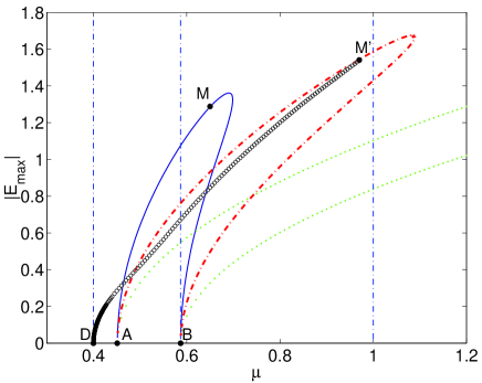
Figure 4: (Color online). Bifurcation diagram of the homogeneous solutions (dotted green curve), 1D-resting CSs (dash-dotted red curve), 2D-resting CSs (solid blue curve), and 1D self-propelled CSs (circles). $|E_{max}|$ corresponds to the maximum field amplitude for localized structures and to the field amplitude for the homogeneous solution. The vertical dash-dotted (blue) lines are the boundaries of the stable and unstable regions of the trivial solution corresponding to B and D and $\mu=1$ in Fig. 2. Parameters are the same as in Fig. 2.

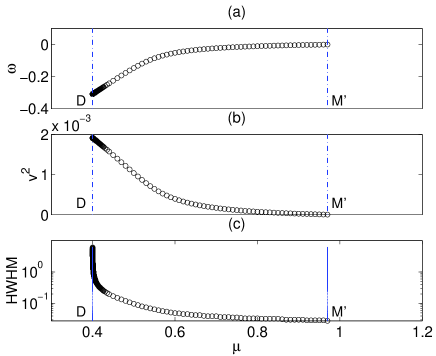
Figure 5: (Color online). Dependencies of the frequency (a), the square of the velocity (b) and the half width at half maximum (HWHM) (c) of the 1D self-propelled CS on the pump current. The vertical lines D and M’ mark the starting point and the end of the branch respectively.

On one side the branch starts from pump current $\mu=\mu_{D}$, where self-propelled CSs appear with zero amplitude (Fig. 4) and with a $k_{max}$ which coincides with the critical transverse wavenumber of the zero solution (intersection of line D and gray (cyan) curve in Fig. 2). Furthermore, self-propelled CSs originate with a negative detuning with respect to the filter central frequency (See Fig. 5(a)), with a finite velocity (Fig. 5(b)) and with an infinite width (Fig. 5(c)). This last characteristic is similar to the appearance of resting CSs in points A and B of Fig. 4 (see also Paulau2008 ). The shape of self-propelled CSs close to point D is displayed in Fig. 6 for $\mu=0.405$. The real part of the field performs many oscillations within a HWHM of a sech-like envelope. The fact that the width diverges while the oscillation wavevector remains finite (corresponding to the critical wavenumber of the zero solution) does not allow to follow the branch close to bifurcation point just by rescaling the spatial length scale. It requires increasing of number of discretization points (2048 points were used in our 1D calculations). As might be expected, it can be proved analytically that in this limit the moving CS is an envelope soliton of the critical traveling-wave solution, and moves with its group velocity.

The moving-CS branch in Fig. 2) defines only existence, and says nothing about stability. It is clear that the entire section of the branch below line B must correspond to unstable CS, because of instability of the zero-amplitude background state. Above line B, we find numerically that the moving cavity solitons are usually stable, though those associated with sidebands may show instability (see section IV).

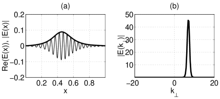
Figure 6: Shape of a moving 1D CS close to the bifurcation point D of Fig. 4. (a) Near field amplitude (solid thick line) and its real part (solid thin line); (b) far field amplitude. $\mu=0.405$.

It is worthwhile to emphasize that the motion of localized states is connected with the modulational instability of the background leading to travelling waves with a finite critical transverse wavevector. This suggests a way of eliminating the drifting instability of resting solitons by removing the finite wavelength instability. This can be done by varying the detuning $\omega_{s}$, which shifts the critical transverse wavevector along the $k_{\perp}$ axis (see Paulau2007 ). If instead we want to enhance the self-propelled solitons (increase the velocity) we need, then, to increase the critical wavenumber.

Increasing the pump, the value of $|k_{max}^{2}|$ and the associated value of $|v|$, decrease (see Fig. 2 and Fig. 5(b)). Simultaneously, the self-propelled CS becomes narrower (Fig. 5 (c)), taller (Fig. 4) and its frequency approaches the one of the filter (Fig. 5 (a)).

The branch of self-propelled CSs ends at point $M^{\prime}$, where the moving solution merges with the resting one (Fig. 4). In fact, at $M^{\prime}$ a drift pitchfork bifurcation takes place. Decreasing $\mu$, two stable self-propelled CSs with velocities $v$ and $-v$ originate from the resting CS that becomes unstable. The squared variables, $v^{2}$ and $k_{max}^{2}$, scale linearly from zero with the distance to the bifurcation point (see Figs. 5(b) and 2), as expected for a supercritical pitchfork.

Finally, some remarks on the 2D case are in order. In 2D, self-propelled CSs can move in any arbitrary direction. The drift is associated to an asymetric cross-section along the the direction of motion while the section in the orthogonal (transverse) direction is symmetric. Due to the lack of rotational symmetry, finding the branch of self-propelled 2D CSs using a Newton method as above requires solving a full 2D problem. This is too demanding computationally for us to obtain a bifurcation diagram to compare with the 1D case. Some 2D results may be inferred, however. Beyond the resting and self-propelled 1D CSs, figure Fig. 4 also shows the resting 2D CS branch (solid (blue) curve) and the homogeneous solutions (dotted (green) curves) from Paulau2008 . Comparing the curves for the 1D and 2D cases one may expect that the 2D self-propelled CS branch will start at the same point $D$, with zero amplitude, infinite width, finite velocity and wavelength equal to the critical transverse wavenumber of the zero solution. Increasing the pump, self-propelled 2D CSs will become narrower and their speed will decrease. The branch of self-propelled 2D CS ends at point $M$ in Fig. 4, where it merges with the resting CS branch. The point M has been obtained from numerical simulations of eqs. (2) for the 2D case Paulau2008 . The natural extension of the drift pitchfork bifurcation observed in 1D to 2D is a drift circle pitchfork bifurcation footnote1 in which a CS moving in an arbitrary direction originates while the resting CS becomes unstable.

IV CS control via feedback phase

In the previous sections we have discussed the properties of model (2) with a fixed feedback phase. However, in delayed systems, the variation of this parameter leads to transitions between adjacent external cavity modes Wolfrum2002 ; Tromborg1984 . Therefore we consider here the influence of feedback phase $\phi$ on the solitonic branches in model (2). In Fig. 7 the solid lines show the branches of resting 1D CSs as a function of $\phi$. The branches have an elliptical shape. The part of the branch with larger amplitude, and lower frequency, is associated to external cavity modes, while the opposite part is associated to anti-modes, saddle points Strogatz that act as separatrices in phase-space. Consider, for instance, the branch shown as a thick line. At $\phi=0$ the higher amplitude CS $Z_{1}$ is stable while the lower amplitude CS $Z_{2}$ is a saddle. As the feedback phase is varied, the amplitude and the frequency of the CS changes continuously. The branch covers a feedback phase interval larger than $4\pi$. Since the feedback phase is $2\pi$ periodic, for some values of the feedback phase six solutions exist, while for others there are only four, as is clear from Fig. 7b.

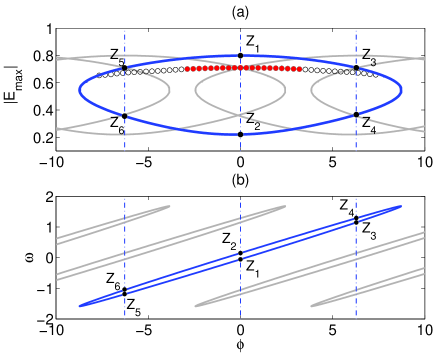
Figure 7: (Color online). Bifurcation diagram of 1D CSs as a function of the feedback phase $\phi$: (a) Maximum amplitude; (b) frequency. The solid thick curve (blue online) corresponds to resting CSs; the open (filled) circles correspond to the unstable (stable) self-propelled CSs. The vertical dashed lines correspond to $\phi=0$, $\phi=\pm 2\pi$. From the $2\pi$ periodicity, translating the thick curves gives the set of equivalent gray curves. Here $\mu=0.6$ and the other parameters as in Fig. 2.

For example, for $\phi=0$, resting CSs $Z_{3}$, $Z_{4}$, $Z_{5}$, $Z_{6}$ exist in addition to $Z_{1}$ and $Z_{2}$. The coexisting “mode” states ($Z_{1}$, $Z_{3}$, $Z_{5}$) have significantly different frequencies, with a separation approximately of $2\pi/\tau\approx 1.25$, similar to the frequency separation of the marginal instability curves in Fig. 2. The coexisting antimodes for a given phase are also associated to neighbor external cavity antimodes ($Z_{2}$ to the central, $Z_{4}$ to the high frequency and $Z_{6}$ to the low frequency one).

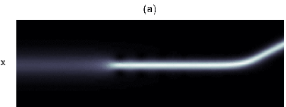
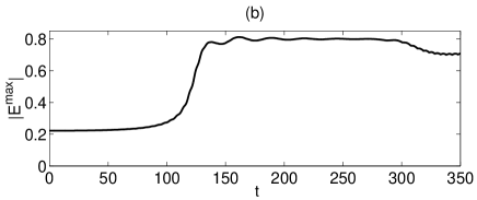
Figure 8: Dynamics of the system (2) for an initial condition just above the point $Z_{2}$ of Fig. 7(a). (a) Time-space plot, where the vertical direction is $x$ and the horizontal direction is time, on the same scale as in panel (b). White corresponds to large amplitude, black to zero. (b) Time evolution of the CS maximum amplitude

.

Changing continuously the feedback phase by $\pm 2\pi$ transforms a CS solution into a different one, associated to an adjacent longitudinal external cavity mode. For example, increasing $\phi$ from $0$ to $2\pi$ transforms $Z_{1}$ into $Z_{3}$. We cannot speak here of multistability because most of these resting solitonic states are unstable for the parameters we have considered. We will show below, however, that these unstable states can be stabilized by the effect of the carrier dynamics in model (1), leading to bistability and apparently to multistability.

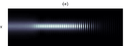
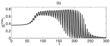
Figure 9: Dynamics of the system, plotted as in Fig. 8, for an initial condition just above the point $Z_{6}$ of Fig. 7(a).

Fig. 7 also shows the branch of self-propelled CSs. Open (filled) circles indicate unstable (stable) solutions. For simplicity we have not plotted here the equivalent solutions obtained for a $2\pi$ shift in the feedback phase. As in the case of resting solitons, there can be multiple moving states and, moreover, they can be bistable because the interval of feedback phases where they are stable is slightly broader than $2\pi$.

Finally Figs. 8 and 9, show two examples of the dynamics of the system starting from an initial condition just above the lower unstable CS branch in Fig. 7(a).

In the first case (Fig. 8) we start the simulation with an initial condition just above point $Z_{2}$ in Fig. 7(a). We observe first a slow evolution away from the lower unstable CS to form a transient approximation to the unstable state $Z_{1}$. We note that $Z_{1}$ differs from initial state in both amplitude and frequency. Then the amplitude and frequency switch to those of the stable self-propelled CS corresponding to the filled (red) circle intersecting the vertical dashed line $\phi=0$ in Fig. 7(a). Such evolution is typical for feedback phase values for which the only stable CS state is the self-propelled CS, and for initial conditions above the lower branch solitonic states.

There is a second scenario, typical for values of the feedback phase for which both the resting and moving upper-branch CSs are unstable. An example is shown in Fig. 9. Starting just above the point $Z_{6}$ the system approaches $Z_{5}$, and then starts oscillating with a large amplitude before switching off completely. This long transient excursion, for a perturbation just above the CS lower branch is an indication of excitable behavior, since perturbations just below this threshold decay directly to the zero solution. The period of the oscillations is close to $\tau$, as might be expected, which indicates that more than one longitudinal mode is excited. Initially, it seems that there is a beating of the two CS modes $Z_{5}$ and $Z_{1}$, but in the later stages the sharpness of the spikes (both dark and, latterly, bright) indicates transient locking of at least three CS modes.

V Influence of carrier dynamics

In this section we address the influence of the carrier lifetime on the dynamics of the system, which is typically very important in semiconductor laser media. For this, we use Eqs. (1) instead of the simplified version (2), studied in previous sections. The resting solitons are actually solutions of both models (2) and (1), because the adiabatic elimination of the carriers does not influence these steady states. As a prototypical example to study the effects of the carrier dynamics on the CS, we will analyze how the stability of state $Z_{1}$ of Fig. 7 changes with the carrier relaxation time $T_{1}$.

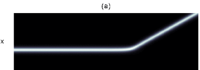
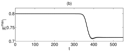
Figure 10: Dynamics of system (1), plotted as in Fig. 8, starting from an initial condition corresponding to the point $Z_{1}$ of Fig. 7. Here $T_{1}=0.05$.

For small enough values $T_{1}<T_{1}^{a}=0.085\pm 0.001$, the behavior of Eqs. (1), starting from the solitonic state $Z_{1}$, differs from the behavior of Eqs. (2) only quantitatively, i.e. we observe in both cases the transition from a resting to a self-propelled CS. Fig. 10 shows this dynamics for $T_{1}=0.05$, which can be compared with the middle and final part of Fig. 8 where a soliton started from $Z_{2}$ first evolves towards $Z_{1}$ and then starts to move.

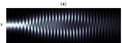
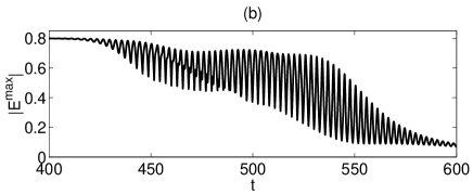
Figure 11: The same as in Fig. 10 for $T_{1}=0.5$.

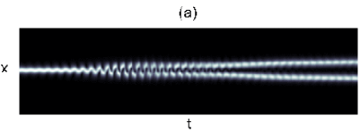
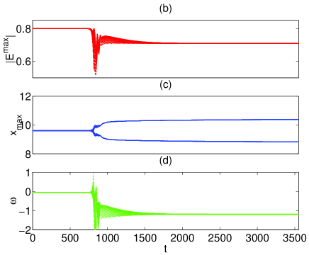
Figure 12: (Color online). Dynamics of the system with the same parameters as in figures 10 and 11, except $T_{1}=1$. (a) Space-time plot of the field amplitude for time interval [750;1000]. (b) Evolution of the CS maximum amplitude; (c) Location of the CS maximum, the split signals the birth of two states; (d) Evolution of the instantaneous CS frequency $\omega=Arg(E_{max}(t)/E_{max}(t-\Delta t))/\Delta t$, all for time interval [0;3500].

For $T_{1}>T_{1}^{a}$, the drifting instability is transformed into a swinging instability, where the CS starts to perform spatial oscillations around its initial position (see Fig. 11a). There are several physical mechanisms that may contribute to this behavior. One is delay, that in combination with the motion of the structure gives a positive feedback at the rear part of the CS, slowing down the motion, and possibly causing the oscillations. Another one is the slow relaxation of the carriers, which also opposes the unidirectional movement of the CS. The oscillations in space are also accompanied by intensity oscillations of the maximum (Fig. 11b). The amplitude of the oscillations grows initially, then evolves in a complex manner before the CS finally switches off. The full quasi-period of the oscillations is again close to $\tau$, indicating multi-mode behavior, though there are two ”maximum maxima” per period, and hence two oscillations in Fig. 11(b) per feedback time. Swinging, followed by switch off, is observed for an interval of carrier relaxation times between $T_{1}^{a}$ and $T_{1}^{b}=0.791\pm 0.001$.

For carrier relaxation times larger than $T_{1}^{b}$ the state $Z_{5}$ becomes stable, and the swinging instability of the state $Z_{1}$ leads to the birth of a pair of solitonic states $Z_{5}$, as shown in Fig. 12. Finally, for $T_{1}>T_{1}^{c}=1.885\pm 0.005$ the state $Z_{1}$ is stable. Moreover, state $Z_{5}$ remains stable, so therefore in this region there is bistability between two resting CSs with different amplitude, which is not found in (2).

For the chosen value of the detuning $\omega_{s}$, and typical values of $T_{1}$, self-propelled self-localized states disappear. However increasing the detuning, which reinforces the drifting instabilities as discussed in Sec. III, we observe stable self-propelled 1D CSs for Eqs. (1) for $T_{1}=1$, $\omega_{s}=200$, $\mu=0.8$, with the other parameters as in Fig. 2. We note that this value of $T_{1}$ is typical Semicond1998 ; Saleh1991 for carrier relaxation in VCSELs.

Summarizing this Section, carrier dynamics plays a really important role in the evolution of the system. For relatively long carrier lifetimes it allows bistability of resting CSs in parameter regimes where it is not present in (2). In an intermediate range of lifetimes it can lead to a new “swinging” CS instability, which in turn may lead to “CS fission”.

VI Final remarks

We have studied in detail the formation of self-propelled localized solutions in a Cavity Soliton Laser composed of a VCSEL subject to filtered external optical feedback. These states are potentially useful for applications such as all-optical delay lines Pedaci2008 . Our results have been obtained for systems with one spatial dimension, but evidence of a qualitative agreement with the more realistic 2D case is given.

The self-propelled soliton branch has been constructed by solving with a Newton method the stationary equations in the reference frame moving with the soliton. The branch originates from the modulational instability bifurcation point of the trivial solution where tilted waves appear with the critical wavenumber. Apparently, amplitude modulation of the tilted wave leads to the existence of self-propelled CSs in such systems.

We have also shown that the characteristics of CSs can be controlled via the feedback phase, and the existence of multiple localized solutions associated to different external cavity modes.

We have analyzed the influence of the carrier relaxation time on the properties of the solitonic states. It has been shown that increasing $T_{1}$ leads to the stabilization of resting solitonic states. This opens the possibility of observing multistability of CSs. For intermediate values of the carrier relaxation time we have observed a new kind of instability leading to the oscillation of the position of the CS and, for larger $T_{1}$, to the formation of two identical solitons at different positions.

Finally, we should mention, that the models used here still represent only a rather rough approximation to experiment. The complexity of real devices is much higher, involving different spatial mechanisms such as carrier diffusion Paulau2004 , gain and loss dispersion Loiko2001 , thermal frequency shift Naumenko2006 , and multiple round-trips in the external cavity Besnard1994 ; Etrich1991 ; Scroggie2009 . Simple models such as ours are, nonetheless, useful for understanding fundamental features of basic phenomena such as self-propelled solitons, and for the prediction of some new phenomena, like the swinging instabilities.

We acknowledge financial support from MICINN (Spain) and FEDER (EU) through Grants No. FIS2007-60327 FISICOS and No. TEC2006-10009 PhoDeCC. We are grateful to T. Ackemann and N.N. Rosanov for useful discussions.

References

- (1) Y. Tanguy, T. Ackemann and R. Jäger, Phys. Rev. A 74, 053824 (2006).
- (2) Y. Tanguy, T. Ackemann, W.J. Firth and R. Jäger, Phys. Rev. Lett. 100, 013907 (2008).
- (3) P.V. Paulau, A.J. Scroggie, A. Naumenko, T. Ackemann, N.A. Loiko, and W. J. Firth, Phys. Rev. E 75, 056208 (2007).
- (4) P.V. Paulau, D. Gomila, T. Ackemann, N.A. Loiko, and W. J. Firth, Phys. Rev. E 78, 016212 (2008).
- (5) www.funfacs.org
- (6) F. Pedaci, S. Barland, E. Caboche, P. Genevet, M. Giudici, J.R. Tredicce, T. Ackemann, A.J. Scroggie, W.J. Firth, G.-L. Oppo, G. Tissoni, R. Jager, Appl. Phys. Lett., 92 011101 (2008).
- (7) A.J. Scroggie, J.M. McSloy, W.J. Firth, Phys. Rev. E, 66,036607 (2002).
- (8) N.N. Rosanov, S.V. Fedorov, A.N. Shatsev, Appl. Phys. B, 81, 937 (2005).
- (9) F. Prati, K. Mahmoud Aghdami, G. Tissoni, M. Brambilla and L. A . Lugiato, ”Moving cavity solitons in a cavity soliton laser based on a VCSEL with saturable absorber”, unpublished.
- (10) M. Giudici, L. Giuggioli, C. Green, and J.R. Tredicce, Chaos, Solitons Fractals 10, 811 (1999).
- (11) M. Yousefi, D. Lenstra, IEEE Journal of Quantum Electronics, 35, 970 (1999).
- (12) A.P.A. Fisher, O.K. Andersen, M. Yousefi, S. Stolte, D. Lenstra, IEEE Journal of Quantum Electronics 36, 375 (2000).
- (13) R. Montagne, E. Hernández-García, A. Amengual, M. San Miguel, Phys. Rev. E, 56, 151 (1997).
- (14) The circle pitchfork bifurcation has been described, for example, in the context of a two species reaction diffusion model Kness .
- (15) M. Kness, L.S. Tuckerman, D. Barkley, Phys. Rev. A 46, 5054 (1992).
- (16) M. Wolfrum, D. Turaev, Opt. Comm. 212, 127 (2002).
- (17) B. Tromborg, J.H. Osmundsen, H. Olesen, IEEE J. Quantum. Electron. 20, P. 1023 (1984).
- (18) S.H. Strogatz, Nonlinear dynamics and chaos with applications to physics, biology, chemistry, and engineering, (Persues books, Reading, Massachusetts, 1994).
- (19) Semiconductor Quantum Optoelectronics. From quantum physics to smart devices, Proceedings of the Fiftieth Scottish Universities Summer School in Physics, St. Andrews, June 1998. Edited by A. Miller, M. Ebrahimzadeh, D.M. Finlayson, (Scottish Universities Summer School in Physics & Institute of Physics, 1999).
- (20) B.E.A. Saleh, M.C. Teich, Fundamentals of Photonics (John Wiley and Sohns, New York, 1991).
- (21) P.V. Paulau, I.V. Babushkin, N.A. Loiko, Phys. Rev. E 70, 046222 (2004).
- (22) N.A. Loiko, I.V. Babushkin, J.Opt.B: Quantum Semiclass. Opt. 3, S234 (2001).
- (23) A. Naumenko, N. Loiko, M. Sondermann, K. Jentsch, T. Ackemann, Opt. Communications, 259, 823 (2006).
- (24) P. Besnard, B. Meziane, K. Ait-Ameur, G. Stephan, IEEE Journal of Quantum electronics, 30, 1713 (1994).
- (25) C. Etrich, A.W. McCord, P. Mandel, IEEE Journal of Quantum electronics, 27, 937 (1991).
- (26) A.J. Scroggie, W.J. Firth, G-L Oppo, Phys. Rev. A 80, 013829 (2009).