Open system effects on slow light and electromagnetically induced transparency

Abstract

The coherence properties of a three-level $\Lambda$-system influenced by a Markovian environment are analyzed. A coherence vector formalism is used and a vector form of the Lindblad equation is derived. Together with decay channels from the upper state, open system channels acting on the subspace of the two lower states are investigated, i.e., depolarization, dephasing, and amplitude damping channels. We derive an analytic expression for the coherence vector and the concomitant optical susceptibility, and analyze how the different channels influence the optical response. This response depends non-trivially on the type of open system interaction present, and even gain can be obtained. We also present a geometrical visualization of the coherence vector as an aid to understand the system response.

I Introduction

A medium that is opaque to radiation on one of the transitions of a $\Lambda$-system can be made transparent by addressing a laser field on the second transition, a phenomenon known as electromagnetically induced transparency (EIT) Fleischhauer et al. (2005); Marangos (1998). Associated with this transparency is an extremely small and dynamically controllable group velocity Hau et al. (1999). The pulse can be brought to a complete stop and stored as an atomic coherence. Most impressive with respect to storage time, is perhaps the storage of a light pulse in a solid for a period greater than one second Longdell et al. (2005). The process can be reversed, and the light pulse released with the original pulse information intact Fleischhauer et al. (2000), making the EIT mechanism a strong candidate to build a quantum memory Fleischhauer and Lukin (2002). Beside applications in quantum information processing, the narrow spectral feature of EIT is an important tool in spectroscopy Krishna et al. (2005), high precision magnetic sensors Katsoprinakis et al. (2006), and atomic clocks Knappe et al. (2004); Vanier (2005). Furthermore, the slow light phenomena can be used for optical delay lines and light storage, but there is a trade-off between the delay of a pulse and the bandwidth Tidström et al. (2007). In order to increase the bandwidth, spatially dispersed light beams in non-isotropic media can be used Dutton et al. (2006).

The above effects depend crucially on the coherence properties of the $\Lambda$-system Arimondo (1996). The dark state superposition, central to the EIT mechanism, is fragile to external influences. This motivates to study open system effects in the dynamics of this system. Open system effects suppress the dark state of the system and thus set the ultimate limit on the storage time of light, the absorption, and the spectral resolution of the transparency. There are tricks that one can play in order to increase the efficiency of this coherence effect. In, for example, Ref. Longdell et al. (2005) the effective decoherence rate was decreased by a method called quantum bang-bang dynamic control, inspired by refocusing techniques in nuclear magnetic resonance Viola and Lloyd (1998).

In this paper, we investigate various types of interactions between the $\Lambda$-system and a Markovian environment modeled by the Lindblad-Kossakowski equation Lindblad (1976); Gorini et al. (1976). Using the coherence vector formalism Lendi (1987); Byrd et al. (2011) we find the asymptotic states ($t\rightarrow\infty$) for the $\Lambda$-system and derive an analytical expression for the corresponding optical response, i.e., the susceptibility of the medium, due to the dephasing, depolarization, and three different amplitude damping channels acting on the two lower states. Effects due to open system interactions are relevant in many experimental instances and depends on the detailed structure of the system, the environment, and the interaction; for possible configurations see, e.g., Fleischhauer et al. (1992); Møller et al. (2008). The approach used here for treating open system effects is general and provides an option for visualization of the system response.

The outline of the paper is as follows. Section II contains a general theory for a Markovian dynamics in a three-level system using coherence vector formalism. In Section III, we apply this framework to a $\Lambda$-system undergoing open system dynamics corresponding to dephasing, depolarization, and amplitude damping channels. The results are presented in Section IV. We give a geometrical visualization of different projections of the steady state solution to the coherence vector when different open systems effects are applied. We derive an analytical expression for the susceptibility in the presence of the open system effects. The paper ends with the conclusions.

II Open three-level system

Let us begin by studying a general three-level quantum system and the effects due to the interaction with a Markovian environment. In this case, the density operator $\hat{\rho}$ satisfies the master equation

$$\partial_{t}\hat{\rho}=\frac{1}{i\hbar}[\hat{H},\hat{\rho}]+\mathcal{\hat{L}}(\hat{\rho}),$$ (1)

where $\hat{H}$ is the Hamiltonian operator. The Liouville superoperator $\hat{\mathcal{L}}$ is linear, describes the coupling with the environment, and can be written on Lindblad form Lindblad (1976)

$$\mathcal{\hat{L}}(\hat{\rho})=\sum_{\mathrm{k}}(\hat{\gamma}_{\mathrm{k}}\hat{\rho}\hat{\gamma}_{\mathrm{k}}^{\dagger}-\tfrac{1}{2}\hat{\gamma}_{\mathrm{k}}^{\dagger}\hat{\gamma}_{\mathrm{k}}\hat{\rho}-\tfrac{1}{2}\hat{\rho}\hat{\gamma}_{\mathrm{k}}^{\dagger}\hat{\gamma}_{\mathrm{k}}),$$ (2)

where $\hat{\gamma}_{\mathrm{k}}$ are Lindblad operators, and the subscript k denotes the open system channels.

For a two-level system it is customary to use a coherence vector representation, called a Bloch-vector representation. Similarly, for a three level system we can write the density matrix $\rho$ and Hamiltonian matrix $H$ in a vector form as Lendi (2007)

$$\rho = \frac{1}{3}\mathds{1}+\,\boldsymbol{x}\cdot\boldsymbol{\lambda},$$

$$H = \hbar\omega_{0}\mathds{1}+\hbar\boldsymbol{\omega}\cdot\boldsymbol{\lambda}.$$ (3)

Here, we have introduced the coherence vector $\boldsymbol{x}=x_{i}{\bf e}_{i}$ (repeated indices summed from now on), the torque vector $\boldsymbol{\omega}=\omega_{i}\boldsymbol{e}_{i}$ associated with the Hamiltonian and the SU(3) matrix generators $\boldsymbol{\lambda}=\lambda_{i}\boldsymbol{e}_{i}$. The basis $\{{\bf e}_{i}\}_{i=1}^{8}$ is real and orthonormal. We have used the standard scalar product ‘ $\cdot$ ’, and $\mathds{1}$ is the $3\times 3$ identity matrix. We use the traceless Gell-Mann matrices $\{\lambda_{i}\}_{i=1}^{8}$ as defined in Ref. Arvind et al. (1997). The length of the coherence vector is $0\leq|\boldsymbol{x}|^{2}\leq 1/3$, with $|\boldsymbol{x}|^{2}=1/3$ for pure states and $|\boldsymbol{x}|^{2}=0$ for maximally mixed states.

By inserting Eq. (II) into Eq. (1) we obtain

$$\dot{\boldsymbol{x}}\cdot\boldsymbol{\lambda} = \frac{1}{i}[\boldsymbol{\omega}\cdot\boldsymbol{\lambda},\boldsymbol{x}\cdot\boldsymbol{\lambda}]+\frac{1}{3}\mathcal{L}(\mathds{1})+\mathcal{L}(\mathbf{\boldsymbol{x}\cdot\boldsymbol{\lambda}}),$$ (4)

i.e., the dynamics reformulated in terms of Gell-Mann matrices. The non-zero form of the Lindblad operators $\hat{\gamma}_{\mathrm{k}}$ is written as $\hat{\gamma}_{\mathrm{k}}\doteq g_{0}\mathds{1}+\boldsymbol{g}_{\mathrm{k}}\cdot\boldsymbol{\lambda}$, where the symbol ‘$\doteq$’ stands for ‘represented by’. In this paper we will not consider the contribution from $g_{0}$ as this term always can be interpreted as an extra contribution to the Hamiltonian foo . Thus, we focus on the ‘Lindblad vectors’ $\boldsymbol{g}_{\mathrm{k}}$.

In Appendix A, we obtain a $\boldsymbol{\lambda}$-independent form of Eq. (4). As a result we obtain the complete dynamics of the system, including open system effects, as an inhomogeneous differential equation Lidar and Schneider (2005)

$$\dot{\boldsymbol{x}}=M\boldsymbol{x}+\boldsymbol{b}$$ (5)

with the evolution matrix $M$ and vector ${\boldsymbol{b}}$ explicitly give in Appendix A. For time-independent and invertible $M$, the general solution of Eq. (5) takes the form Lendi (1987, 2007)

$$\boldsymbol{x}=e^{Mt}\boldsymbol{x}_{0}-M^{-1}\boldsymbol{b},$$ (6)

where $\boldsymbol{x}_{0}=\boldsymbol{x}(0)+M^{-1}\boldsymbol{b}$, $\boldsymbol{x}(0)$ being the initial coherence vector.

The evaluation of the exponential of $M$ is non-trivial, since $M$ is not diagonalizable in general. To deal with this fact one may resort to the Jordan normal form of $M$, i.e., $M=SJS^{-1}$, where $J$ has non-zero entries only on the diagonal and the super-diagonal, and $S$ is an invertible matrix. Expanding the exponent in Eq. (6), we can write the general solution as

$$\boldsymbol{x}=Se^{Jt}S^{-1}\boldsymbol{x}_{0}-M^{-1}\boldsymbol{b}.$$ (7)

The real part of the eigenvalues $\{s_{j}\}_{j=1}^{8}$, $s_{j}\in C$, of $M$ originates from $\hat{\mathcal{L}}$ and must be zero or negative in order to preserve non-negativity of the density operator.

We now look at the eigenvectors of $M$. Higher-dimensional Jordan Blocks occur provided $M$ has linearly dependent eigenvectors corresponding to degenerate eigenvalues. However, in all the cases we investigate in this paper we only identify one-dimensional Jordan blocks.

We now ask what happens for different open system effects corresponding to one-dimensional Jordan blocks. We focus on the case where we have $s_{i\in I}=0$, $I$ being an index set, and $\mathrm{Re}(s_{i\notin I})<0$. In the $t\rightarrow\infty$ limit, the matrix $e^{Jt}$ tends to the matrix $P^{\prime}$, which projects onto the subspace corresponding to $I$. Thus, in this limit, $e^{Mt}=Se^{Jt}S^{-1}$ tends to the projector $SP^{\prime}S^{-1}$ and the asymptotic coherence vector ${\boldsymbol{x}}^{(\infty)}$ depends on the initial coherence vector ${\boldsymbol{x}}_{0}$ according to

$${\boldsymbol{x}}^{(\infty)}=P{\boldsymbol{x}}_{0}-M^{-1}{\boldsymbol{b}}.$$ (8)

For the cases studied in this paper, $I$ is the empty set, i.e., $\mathrm{Re}(s_{i})<0\ \forall i$, we have $e^{Mt}=Se^{Jt}S^{-1}\rightarrow 0$ when $t\rightarrow\infty$. In this case, the asymptotic state is determined by

$${\boldsymbol{x}}^{(\infty)}=-M^{-1}{\boldsymbol{b}},$$ (9)

thus being independent of ${\boldsymbol{x}}_{0}$. Further discussions on the existence and properties of asymptotic states in Markovian open quantum systems can be found in Refs. Ticozzi and Viola (2007, 2009); Schirmer and Wang (2010).

III Open $\Lambda$-system

Figure 1: The $\Lambda$-system. The field on the $a$-$b$ transition is the weak probe field $\Omega_{b}$, and the field on the $a$-$c$ transition is the control field $\Omega_{c}$. The upper level is broadened by the finite lifetime $1/\gamma$.

An electromagnetic field interacting with matter gives rise to a matter polarization. The linear part of the polarization field $P=P(E)$ can be written in terms of the electrical susceptibility $\chi=P/(E\epsilon_{0})$, with $\epsilon_{0}$ the electrical permittivity in free space. The real and imaginary parts of the susceptibility describe the phase velocity of the electrical field and the absorption or gain of the field, respectively. The macroscopic polarization field of an isotropic medium consisting of $N$ atoms per unit volume is $\mathbf{P}\equiv\langle\hat{\mathbf{P}}\rangle=N\langle\hat{\mathbf{p}}\rangle=N\mathrm{Tr}[\hat{\rho}\hat{\boldsymbol{\mu}}],$ where $\hat{\rho}$ is the density operator and $\hat{\boldsymbol{\mu}}=e\,\hat{\mathbf{r}}$ is the dipole operator with electric charge $e$ and position operator $\hat{\mathbf{r}}$. Therefore, if $\hat{\rho}$ is known as a function of the optical field, the optical response is too, as it is given by the coherences of $\hat{\rho}$. In this section we develop the tools to compute $\hat{\rho}$ for an open $\Lambda$-system and in the next section we find the resulting optical response $\chi$.

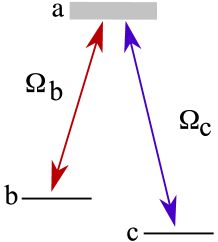
The $\Lambda$-system consists of two ground state levels coupled to an excited state via electromagnetic fields, as shown in Fig. 1. The corresponding Hamiltonian is given by $\hat{H}(t)=\hat{H}_{0}-\hat{\boldsymbol{\mu}}\cdot\mathbf{E}(t)$, where $\hat{H}_{0}$ is the Hamiltonian of the bare atom, $\hat{\boldsymbol{\mu}}$ is the electric dipole operator, and $\mathbf{E}(t)$ is an oscillating electric field. Furthermore, let $\mathcal{E}_{i}$ be the energy eigenvalues of $\hat{H}_{0}$ corresponding to the bare eigenstates $|i\rangle$, $i=a,b,c$. In a frame rotating with the external field, the Hamiltonian operator reads

$$\hat{H}=\hbar\,\delta_{b}|b\rangle\langle b|+\hbar\,\delta_{c}|c\rangle\langle c|-\hbar\,\Omega_{b}|a\rangle\langle b|-\hbar\,\Omega_{c}|a\rangle\langle c|+h.c.,$$ (10)

where we have used the rotating wave approximation and we have defined the complex Rabi frequencies in terms of the electric field $\mathbf{E}$ in the rotating frame as $\Omega_{i}=\langle a|{\hat{\boldsymbol{\mu}}}|i\rangle\cdot\mathbf{E}/(2\hbar)$ and detunings $\delta_{i}=\omega_{i}-(\mathcal{E}_{a}-\mathcal{E}_{i})/\hbar$, where $\omega_{i}$ are the frequencies of the field. Note the factor 1/2 in the definition of $|\Omega_{i}|$, introduced for notational convenience. Defining the Gell-Mann matrices in terms of the basis ordered as $\{|b\rangle,|c\rangle,|a\rangle\}$, the parameters of the Hamiltonian matrix in Eq. (3) are given by

$$\omega_{0} =\frac{1}{3\hbar}\mathrm{Tr}[H]=\frac{2}{3}\Delta,$$

$$\boldsymbol{\omega} =\frac{1}{2\hbar}\mathrm{Tr}[H\lambda_{i}]\boldsymbol{e}_{i}=\delta{\boldsymbol{e}}_{3}-|\Omega_{b}|\cos\phi_{b}{\boldsymbol{e}}_{4}-|\Omega_{b}|\sin\phi_{b}{\boldsymbol{e}}_{5}-|\Omega_{c}|\cos\phi_{c}{\boldsymbol{e}}_{6}-|\Omega_{c}|\sin\phi_{c}{\boldsymbol{e}}_{7}-\frac{1}{\sqrt{3}}\Delta{\boldsymbol{e}}_{8},$$ (11)

where $\Omega_{i}=|\Omega_{i}|\exp(i\phi_{i})$ and we have defined the two-photon detuning $\delta=(\delta_{b}-\delta_{c})/2$ as well as the mean detuning $\Delta=(\delta_{b}+\delta_{c})/2$.

We now specify the Lindblad operators that describe the different forms of open system dynamics. Spontaneous emission corresponding to the amplitude damping of the excited energy state $|a\rangle$ to either of the two ground states $|b\rangle$ or $|c\rangle$ with rates $\gamma_{b}$ and $\gamma_{c}$ is assumed to be always present. The corresponding Lindblad operators and their matrix representation read

$$\hat{\gamma}_{b} = \sqrt{\gamma_{b}}|b\rangle\langle a|\doteq\frac{1}{2}\sqrt{\gamma_{b}}(\lambda_{4}+i\lambda_{5}),$$

$$\hat{\gamma}_{c} = \sqrt{\gamma_{c}}|c\rangle\langle a|\doteq\frac{1}{2}\sqrt{\gamma_{c}}(\lambda_{6}+i\lambda_{7}),$$ (12)

and they define the natural line width $\gamma\equiv\gamma_{b}+\gamma_{c}$ indicated in Fig. 1. The subscripts $b$ and $c$ indicate the final quantum state of the atom after interaction with the environment through the decay channel. The corresponding Lindblad vectors are

$$\boldsymbol{g}_{b} = \frac{1}{2}\sqrt{\gamma_{b}}(\boldsymbol{e}_{4}+i\boldsymbol{e}_{5}),$$

$$\boldsymbol{g}_{c} = \frac{1}{2}\sqrt{\gamma_{c}}(\boldsymbol{e}_{6}+i\boldsymbol{e}_{7}).$$ (13)

These vectors are complex-valued and therefore $C^{(-)}$ in Eq. (43) is non-vanishing and, accordingly, the decay channel contributes to the dynamics, Eq. (5), with a non-zero ${\boldsymbol{b}}$.

The dark state of the $\Lambda$-system is

$$|d\rangle=\frac{1}{\sqrt{|\Omega_{b}|^{2}+|\Omega_{c}|^{2}}}(\Omega_{c}^{*}|b\rangle-\Omega_{b}^{*}|c\rangle).$$ (14)

This is an eigenstate of the Hamiltonian, which is unaffected by the decay channels defined by Eq. (III). The additional open system effects that we are primarily interested in are the ones that act on the two-dimensional subspace $V_{bc}=\{|b\rangle,|c\rangle\}$, since these could potentially destroy the dark state and the associated phenomena. We consider the limit of a weak probe field and a strong control field, i.e., $|\Omega_{b}|\ll|\Omega_{c}|$, hence the dark state will be close to $|b\rangle$.

Although a continuum set of channels is necessary to fully cover all possible cases Bacon et al. (2001); Lloyd and Viola (2001), it is known Nielsen and Chuang (2000) that depolarization, dephasing, and amplitude damping constitute a set of channels that captures essential features of open system effects for two-level systems. Here, we examine these channels acting on $V_{bc}$. Depolarization and dephasing are particular combinations of the Hermitian Lindblad operators

$$\hat{\gamma}_{x} = \sqrt{\eta_{x}}(|b\rangle\langle c|+|c\rangle\langle b|)\doteq\sqrt{\eta_{x}}\lambda_{1},$$

$$\hat{\gamma}_{y} = \sqrt{\eta_{y}}(-i|b\rangle\langle c|+i|c\rangle\langle b|)\doteq\sqrt{\eta_{y}}\lambda_{2},$$

$$\hat{\gamma}_{z} = \sqrt{\eta_{z}}(|b\rangle\langle b|-|c\rangle\langle c|)\doteq\sqrt{\eta_{z}}\lambda_{3},$$ (15)

where the symbols $\eta_{k}$ are used to denote rates of the various channels acting on $V_{bc}$. The corresponding Lindblad vectors are real and given by

$$\boldsymbol{g}_{x} =\sqrt{\eta_{x}}\boldsymbol{e}_{1},$$

$$\boldsymbol{g}_{y} =\sqrt{\eta_{y}}\boldsymbol{e}_{2},$$

$$\boldsymbol{g}_{z} =\sqrt{\eta_{z}}\boldsymbol{e}_{3}.$$ (16)

The depolarization channel is isotropic, i.e., corresponds to $\eta_{x}=\eta_{y}=\eta_{z}\equiv\eta/3$. The dephasing channel, on the other hand, is anisotropic and corresponds to $\eta_{x}=\eta_{y}=0,\eta_{z}\neq 0$. Neither depolarization nor dephasing contribute to ${\boldsymbol{b}}$ since $C^{(-)}$ vanishes.

As already stated, the dark state is close to $|b\rangle$ when the intensity of the probe field is much smaller than the intensity of the control field. Because of this we expect a non-vanishing amplitude damping $b\leftarrow c$ to influence the $\Lambda$-system in a different manner as compared to the channel $c\leftarrow b$. To examine this quantitatively, we study the following channels

$$\hat{\gamma}_{bc}=\sqrt{\eta_{bc}}|b\rangle\langle c|\doteq\frac{1}{2}\sqrt{\eta_{bc}}(\lambda_{1}+i\lambda_{2}),$$

$$\hat{\gamma}_{cb}=\sqrt{\eta_{cb}}|c\rangle\langle b|\doteq\frac{1}{2}\sqrt{\eta_{cb}}(\lambda_{1}-i\lambda_{2}),$$ (17)

where $\hat{\gamma}_{bc}$ flips $|c\rangle$ to $|b\rangle$ at a rate $\eta_{cb}$ and vice versa for $\hat{\gamma}_{cb}$. The corresponding Lindblad vectors read

$$\boldsymbol{g}_{bc} =\frac{1}{2}\sqrt{\eta_{bc}}(\boldsymbol{e}_{1}+i\boldsymbol{e}_{2}),$$

$$\boldsymbol{g}_{cb} =\frac{1}{2}\sqrt{\eta_{cb}}(\boldsymbol{e}_{1}-i\boldsymbol{e}_{2}),$$ (18)

which are complex-valued and may therefore contribute to ${\boldsymbol{b}}$.

The evolution matrix $M$ and the vector $\boldsymbol{b}$ are obtained by summing the contributions from the above described open system channels. We may write the resulting $M$ in a simple form by applying the following similarity transformation

$$M=R^{-1}M^{\prime}R,$$ (19)

where

$$R=\boldsymbol{e}_{1}^{\phantom{\mathrm{T}}}\!\boldsymbol{e}_{1}^{\mathrm{T}}+\boldsymbol{e}_{2}^{\phantom{\mathrm{T}}}\!\boldsymbol{e}_{2}^{\mathrm{T}}+\boldsymbol{e}_{3}^{\phantom{\mathrm{T}}}\!\boldsymbol{e}_{3}^{\mathrm{T}}+\boldsymbol{e}_{5}^{\phantom{\mathrm{T}}}\!\boldsymbol{e}_{4}^{\mathrm{T}}+\boldsymbol{e}_{6}^{\phantom{\mathrm{T}}}\!\boldsymbol{e}_{5}^{\mathrm{T}}+\boldsymbol{e}_{7}^{\phantom{\mathrm{T}}}\!\boldsymbol{e}_{6}^{\mathrm{T}}+\boldsymbol{e}_{8}^{\phantom{\mathrm{T}}}\!\boldsymbol{e}_{7}^{\mathrm{T}}+\boldsymbol{e}_{4}^{\phantom{\mathrm{T}}}\!\boldsymbol{e}_{8}^{\mathrm{T}}.$$ (20)

The transformed evolution matrix $M^{\prime}$ takes the block structure form

$$M^{\prime}=\begin{pmatrix}A&C\\ -C^{\mathrm{T}}&B\end{pmatrix}$$ (21)

with the submatrices

$$A = \begin{pmatrix}-\mathrm{Re}(\Gamma)&-\mathrm{Im}(\Gamma)&0&0\\ \mathrm{Im}(\Gamma)&-\mathrm{Re}(\Gamma)&0&0\\ 0&0&-\eta_{{}_{+}}&\tfrac{\eta_{{}_{-}}\!-\gamma_{\mathrm{m}}}{\sqrt{3}}\\ 0&0&0&-2\gamma\\ \end{pmatrix},$$

$$B = \begin{pmatrix}-\mathrm{Re}(\Gamma_{-})&-\mathrm{Im}(\Gamma_{-})&0&0\\ \mathrm{Im}(\Gamma_{-})&-\mathrm{Re}(\Gamma_{-})&0&0\\ 0&0&-\mathrm{Re}(\Gamma_{+})&-\mathrm{Im}(\Gamma_{+})\\ 0&0&\mathrm{Im}(\Gamma_{+})&-\mathrm{Re}(\Gamma_{+})\\ \end{pmatrix},$$

$$C = \begin{pmatrix}|\Omega_{c}|\sin\phi_{c}&-|\Omega_{c}|\cos\phi_{c}&|\Omega_{b}|\sin\phi_{b}&-|\Omega_{b}|\cos\phi_{b}\\ |\Omega_{c}|\cos\phi_{c}&|\Omega_{c}|\sin\phi_{c}&-|\Omega_{b}|\cos\phi_{b}&-|\Omega_{b}|\sin\phi_{b}\\ |\Omega_{b}|\sin\phi_{b}&-|\Omega_{b}|\cos\phi_{b}&-|\Omega_{c}|\sin\phi_{c}&|\Omega_{c}|\cos\phi_{c}\\ \sqrt{3}|\Omega_{b}|\sin\phi_{b}&-\sqrt{3}|\Omega_{b}|\cos\phi_{b}&\sqrt{3}|\Omega_{c}|\sin\phi_{c}&-\sqrt{3}|\Omega_{c}|\cos\phi_{c}\end{pmatrix}.$$ (22)

Here, we have introduced the parameters

$$\gamma_{\mathrm{m}} = \gamma_{b}-\gamma_{c},$$

$$\eta_{{}_{\pm}} = \eta_{bc}\pm\eta_{cb},$$

$$\Gamma = 2i\delta+(\eta_{{}_{+}}+8\eta+4\eta_{z})/2,,$$

$$\Gamma_{\pm} = i(\delta\mp\Delta)+\gamma_{\pm},$$

$$\gamma_{\pm} = \gamma+(6\eta+2\eta_{z}+\eta_{{}_{+}}\pm\eta_{{}_{-}})/4.$$ (23)

The diagonal elements of $M^{\prime}$ are real and negative, and contain the open system rates. The only off-diagonal element containing open system effects is $(\eta_{{}_{-}}-\gamma_{\mathrm{m}})/\sqrt{3}$ in $A$. They are non-vanishing if the amplitude damping rates in $V_{bc}$, and also if the decay rate from the exited state to the ground states, are unbalanced. This fact also influences $\boldsymbol{b}$, which is explicitly given by

$$\boldsymbol{b}=\frac{2\eta_{{}_{-}}+\gamma_{\mathrm{m}}}{6}\boldsymbol{e}_{3}+\frac{\gamma}{2\sqrt{3}}\boldsymbol{e}_{8}.$$ (24)

Thus, $\boldsymbol{b}$ is non-vanishing if damping processes are present in the open system dynamics.

IV Results

We begin by analyzing the asymptotic state of the quantum system as represented by the coherence vector ${\boldsymbol{x}}^{(\infty)}$. The use of the asymptotic coherence vector is justified by its relation to measurable quantities. For instance, two of its components determine the real and imaginary parts of the induced electric polarization according to $P_{ab}=N\mu_{ab}\rho_{ab}^{(\infty)}=N\mu_{ab}(x_{4}^{(\infty)}+ix_{5}^{(\infty)})$, from which the susceptibility of the probe field can be found.

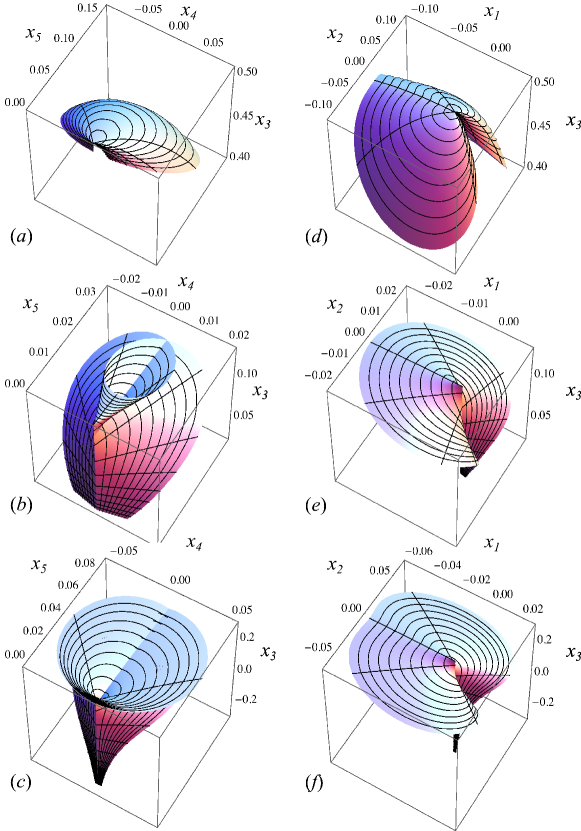
In Fig. 2, we show the projection of the eight-dimensional coherence vector space onto three-dimensional cuts for the cases of depolarization and amplitude damping $c\leftarrow b$ channels, and compare with the ideal case where decay of the excited state $|a\rangle$ to the two ground states $|b\rangle$ and $|c\rangle$ are the only open system effects present. The two parameters spanning the surface are the probe field strength $\Omega_{b}$ and the two photon detuning $\delta$; the control field strength $\Omega_{c}$ is held constant.

The components $x_{1},x_{2}$, and $x_{3}$ shown in Fig. 2(d-f), concern the coherence of the asymptotic state in the $V_{bc}$ subspace. Components 1 and 2 are the real and imaginary part of the coherence $\rho_{bc}$, i.e., they describe the phase relation between the $|b\rangle$ and $|c\rangle$ amplitudes of the asymptotic state. The third component $x_{3}$ is the corresponding population balance. Fig. 2(d) shows the ideal case at zero detuning. Here, $x_{1}$ is negative, $x_{2}$ is zero, and $x_{3}$ is close to 0.5. This is precisely the dark state with a real and negative coherence between the $|b\rangle$ and $|c\rangle$ amplitudes, and most of the population in $|b\rangle$. For non-zero detuning, we can visualize how the dark state deteriorates, by inspecting the entire surface. Depolarization is added in Fig. 2(e). In this case, we see how the $x_{3}$ component radically changes towards a more balanced population and the magnitudes of the coherences $x_{1}$ and $x_{2}$ decrease, as compared to the ideal case. This can be understood physically as the depolarization channel drives the system towards a balanced mixture in the $V_{bc}$ subspace. Similar effects occur for the case of the $c\leftarrow b$ channel, shown in Fig. 2(f).

The components $x_{3},x_{4}$, and $x_{5}$ shown in Fig. 2(a-c) are directly related to the optical response of the atom to the probe field. A zero detuned ideal case is characterized by vanishing $x_{4}$ and $x_{5}$. This implies that the electric polarization vanishes, clearly demonstrating the EIT effect. By adding depolarization, the $x_{5}$ component becomes positive at zero detuning and therefore absorption is present, as shown in Fig. 2(b). The $c\leftarrow b$ amplitude damping channel, shown in Fig. 2(c), gives rise to a negative $x_{5}$ component, corresponding to probe field gain.

Figure 2: Plots of the asymptotic state for two different cuts through the eight dimensional coherence vector space is shown: $x_{4}$, $x_{5}$, $x_{3}$ coordinates of the asymptotic state in (a-c) and $x_{1}$, $x_{2}$, $x_{3}$ coordinates of the asymptotic state in (d-f). Different open system channels are shown: ideal case in (a,d), depolarization $\eta=0.2$ in (b,e), and amplitude damping $c\leftarrow b$ channel $\eta_{cb}=0.2$ in (c,f). Radial mesh corresponds to changing $\Omega_{b}$ from 0 to 0.1 in steps of 0.02, tangential mesh corresponds to the two-photon detuning $-5$ to 5 in steps of 0.5; the exception is (a) where the interval is given between $-$5 to 0. Other parameter values are $\Omega_{c}=1$, $\gamma=1$ and $\Delta=0$.

Let us now examine the susceptibility for a small probe field that interacts with a medium consisting of a collection of $\Lambda$-systems that in turn are affected by the open system channels considered in Sec. III. The susceptibility Boyd (2003), of a medium is related to the asymptotic state of the atomic coherence $\rho_{ab}^{(\infty)}=x_{4}^{(\infty)}+ix_{5}^{(\infty)}$, which can be calculated by Eq. (9) using Eqs. (21) and (24). Explicitly,

$$\chi=\lim_{\Omega_{b}\rightarrow 0}\kappa\frac{\partial}{\partial\Omega_{b}}\rho_{ab}^{(\infty)}$$ (25)

with $\kappa=N|\langle a|{\hat{\boldsymbol{\mu}}}|b\rangle|^{2}/(2\epsilon_{0}\hbar)$, and we recall that the Rabi frequency is defined in a non-standard way with an extra factor of $2$ for notational convenience. The expression of the susceptibility in Eq. (25) holds in the limit of a small probe field. Furthermore, we recall that the real part of the susceptibility is related to the phase evolution of the optical field, while the imaginary part describes the absorption or gain.

The open system channels defined by the Lindblad vectors in Eqs. (III), (III), and (III), change the properties of the $\Lambda$-system in a nontrivial way. The susceptibility in the general case can be calculated from Eq. (9) and we find

$$\chi=i\kappa\frac{\gamma/2\,\left(\eta_{{}_{-}}+\eta_{{}_{+}}\right)|\Gamma_{+}|^{2}\Gamma^{*}+\Big{[}\left(\gamma+\gamma_{\mathrm{m}}+2\eta_{{}_{-}}\right)\mathrm{Re}(\Gamma_{+})\Gamma^{*}+\gamma(\eta_{{}_{-}}-\eta_{{}_{+}})\Gamma_{+}^{*}\Big{]}|\Omega_{c}|^{2}}{\left(\Gamma_{-}^{*}\Gamma^{*}+|\Omega_{c}|^{2}\right)\Big{[}\gamma\eta_{{}_{+}}|\Gamma_{+}|^{2}+\left(\gamma+\gamma_{\mathrm{m}}-\eta_{{}_{-}}+3\eta_{{}_{+}}\right)\mathrm{Re}(\Gamma_{+})|\Omega_{c}|^{2}\Big{]}},$$ (26)

where the parameters are defined in Eq. (III). It should be noted that this expression contains all information of the detunings and phases of the optical fields, as well as the effects due to any combination of depolarization, dephasing, and $b\leftrightarrow c$ channels. Hence, the linear susceptibility of the probe field is obtained for any point in parameter space spanned by all of the above mentioned parameters, assuming only the validity of the Lindblad equation and the rotating wave approximation.

In the following we use Eq. (26) to study the susceptibility due to the different open system effects. The analytical expressions below are retrieved from Eq. (26) as special cases by setting all channel rates except one to zero. We assume the non-zero channel rate $\eta_{k}$ to be much smaller than the decay rate, i.e., $\eta_{k}\ll\gamma$, and a Rabi frequency strong enough to establish EIT, i.e., $\eta_{k}\gamma\ll|\Omega_{c}|^{2}$. Furthermore, we assume zero mean detuning $\Delta=0$, a balanced decay $\gamma_{\mathrm{m}}=0$, and that the two-photon detuning is not much larger than $|\Omega_{c}|$.

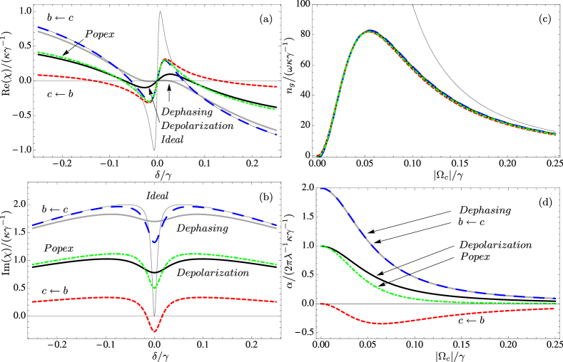
In Figs. 3(a) and 3(b) we show the susceptibility for different open system channels, using the same rate for all open system channels. Since the susceptibility is a complex function, the real and imaginary parts are plotted separately. Note that in the figures we use the exact expression in Eq. (26).

If we put all channel rates to zero except $\eta_{z}$ we obtain the susceptibility

$$\chi_{\mathrm{dephase}}=\kappa\frac{2\delta+2i\eta_{z}}{|\Omega_{c}|^{2}-\delta(2\delta+i\gamma)}.$$ (27)

This expression for the susceptibility is frequently encountered in the literature, see, e.g., Ref. Scully and Zubairy (1997).

If we put $\eta_{{}_{-}}=\eta_{{}_{+}}=\eta_{bc}\neq 0$ we find the susceptibility of a medium that effectively takes population from $|c\rangle$ to $|b\rangle$. We have,

$$\chi_{b\leftarrow c}=\kappa\frac{2\delta+i\eta_{bc}/2}{|\Omega_{c}|^{2}-\delta(2\delta+i\gamma)}.$$ (28)

This expression for the susceptibility is also frequently encountered in the literature, see, e.g., Ref. Gea-Banacloche et al. (1995). It is interesting to note the similarity of this expression with Eq. (27), although the open system channels are quite different. Nevertheless, in Figs. 3(a) and 3(b) it can be seen that the phase response of $\chi_{b\leftarrow c}$ is larger than for $\chi_{\mathrm{dephase}}$. This means that a medium affected by pure dephasing cannot slow down light as efficiently as compared to a medium affected by the $b\leftarrow c$ channel, assuming that the channel rates are equal.

We now consider the amplitude damping channel in the $c\leftarrow b$ direction. The expression of the susceptibility in this case reads

$$\chi_{c\leftarrow b}=\kappa\frac{2\delta-i\eta_{cb}/2}{|\Omega_{c}|^{2}-\delta(2\delta+i\gamma)}.$$ (29)

This channel shows a different behavior compared to all other considered channels, it shows gain where the other channels show absorption. That is, a slowly propagating light pulse will be amplified due to the interaction with the environment described by the $c\leftarrow b$ channel.

Let us now consider amplitude damping channels with equal rates in both directions in the subspace $V_{bc}$, corresponding to the non-zero parameters $\eta_{bc}=\eta_{cb}\equiv\eta_{pe}$. This open system channel may be important in experimental situations where, e.g., atoms collide and the populations of the states undergo sudden incoherent exchange. We denote this as the population exchange channel ‘popex’. We obtain,

$$\chi_{\mathrm{popex}}=\kappa\frac{2\delta+i\gamma\eta_{pe}^{2}/(8|\Omega_{c}|^{2})}{|\Omega_{c}|^{2}-\delta(2\delta+i\gamma)}.$$ (30)

As expected, the absorption profile is located in between the profiles of $\chi_{b\leftarrow c}$ and $\chi_{c\leftarrow b}$, as can be seen in Fig. 3(b). To first order, the absorption profiles of the different amplitude damping channels is shifted by the parameter $\eta_{{}_{-}}$. However, the phase response, i.e., $\mathrm{Re}\left(\chi_{b\leftarrow c}\right)$ is not affected by this shift, and it is approximately the same for all considered amplitude damping channels.

The susceptibility associated with the isotropic depolarization channel ($\eta\neq 0$) is given by

$$\chi_{\mathrm{depol}}=\kappa\frac{2\delta+2i\eta/3}{|\Omega_{c}|^{2}-\delta(2\delta+i\gamma)}.$$ (31)

In experiments, e.g., where one uses laser beams and hot atomic gases, this open system interaction is relevant as it corresponds to coherently prepared atoms leaving the laser beam, replaced with atoms in a completely mixed quantum state. The susceptibility is plotted in Fig. (3) and it can be seen that the phase response $\mathrm{Re}\left(\chi_{\mathrm{depol}}\right)$ is located between the corresponding curves for the dephasing and the amplitude damping channels. Furthermore, the absorption curve $\mathrm{Im}\left(\chi_{\mathrm{depol}}\right)$ is close to the absorption profile of the depolarization channel, but significantly smaller than the corresponding curves for the dephasing and $b\leftarrow c$ channels. With respect to absorption and phase response, the depolarization channel is therefore not as harmful as the dephasing channel.

Figure 3: (Color online) In (a) and (b) we show the real and imaginary part of the susceptibility. In (c) and (d) the slow-down factor (group index) $n_{g}$ and absorption $\alpha$ at two-photon resonance, are shown as a function of the control field $|\Omega_{c}|$. The thin black line shows the case of no open system interaction on $V_{bc}$. The thick gray line shows the dephasing channel and the thick black line shows the depolarization channel. The remaining lines describe three versions of the amplitude damping channel: the wide-dashed (blue) line shows the $b\leftarrow c$ damping channel, the dashed (red) line shows the $c\leftarrow b$ damping channel, and the dash-dotted (green) line shows the population exchange channel (popex), i.e., the incoherent sum of the two damping channels with equal rate. In all plots the proportionality factor $\kappa$ defined below Eq. (25) is scaled to 1. In (a) and (b) the parameter values are $|\Omega_{c}|=0.16$, $\gamma=1$, $\Delta=0$, and all non-zero channel rates are set equal to $0.1$. In (c) and (d) the channel rates are normalized so that the slow-down factors are matched.

When there is no open system interaction on $V_{bc}$ we retrieve the ideal susceptibility,

$$\chi_{\mathrm{ideal}}=\kappa\frac{2\delta}{|\Omega_{c}|^{2}-\delta(2\delta+i\gamma)},$$ (32)

included in Fig. (3) as a reference.

Often one is interested in achieving the slowest possible group velocity in a medium consisting of $\Lambda$-systems. The slow-down factor, or group index, is proportional to the derivative of the real part of the susceptibility $n_{g}\equiv\omega\partial_{\delta}\mathrm{Re}\left(\chi\right)/2$ at angular frequency $\omega$. To compare the absorption for a given slow-down factor at $\delta=\Delta=0$ we normalize the channel rates to give the same slow-down factor. Approximating $\partial_{\delta}\chi$ for small channel rates in $V_{bc}$ gives

$$\partial_{\delta}\mathrm{Re}\left(\chi\right)\big{|}_{\delta=\Delta=0} \approx\kappa\frac{2|\Omega_{c}|^{2}-\gamma\left(\frac{8\eta}{3}+\eta_{bc}+\eta_{cb}+2\eta_{pe}+4\eta_{z}\right)}{|\Omega_{c}|^{4}}$$ (33)

thus, the normalized rates are $\eta_{z}=\eta_{bc}/4=\eta_{cb}/4=\eta_{pe}/2=2\eta/3$. Using these normalized rates, we plot the slow-down factor as a function of the control field in Fig. 3(c) to verify that they are equal. The absorption coefficient is defined as $\alpha=(2\pi/\lambda)\mathrm{Im}\left(\chi\right)$. In Fig. 3(d) we show the absorption on two-photon resonance as a function of the control field. We see that the different open system channels give different absorption profiles, even though the slow-down factors are equal in this regime. Furthermore, it is interesting to note that the dephasing and the $b\leftarrow c$ amplitude damping channels, with normalized channel rates, have identical absorption characteristics. We see that the isotropic depolarization and population exchange channels are quite similar in Fig. 3(d), but more essentially, they have a lower absorption than the dephasing and the $b\leftarrow c$ amplitude damping channels. As already mentioned, the $c\leftarrow b$ damping is special in that it yields a gain where the other channels yield absorption of the probe field.

V Conclusions

We analyze a three-level $\Lambda$-system interacting with a Markovian environment. The Lindblad master equation is reformulated using the Gell-Mann matrices as a basis. We rewrite this in a convenient vector formalism that is independent of the specific matrix representation of the SU(3) generators. An evolution matrix corresponding to this vector form is worked out in detail and the dynamics is written as an affine-linear matrix differential equation. The general solution of this equation can be given in terms of the Jordan normal form. The Jordan blocks of the evolution matrix are generically one-dimensional and the real part of the spectrum is negative. From this follows that the asymptotic solution in all cases we are interested in are independent of the initial states and given by the inverse of the evolution matrix multiplied by a vector that is given by the open system interaction.

The linear optical response of a quantum system is given by the asymptotic steady state solution of the evolution equation. We find an explicit and closed analytical form of the susceptibility for general open system dynamics, including pure dephasing, depolarization, and three different forms of amplitude damping channels.

The open system effects introduce a non-trivial behavior of the linear optical response of the $\Lambda$-system. For example, we show that the isotropic depolarization channel is less detrimental to the induced transparency and the corresponding slow-down effect, than is pure dephasing. Furthermore, an amplitude damping channel can lead to reduced absorption and even gain for the probe field.

Appendix A

In this Appendix, we provide a detailed derivation of the evolution matrix $M$ and the vector $\boldsymbol{b}$ for Lindblad-type master equations of a three-level system. Define the vector products

$$\boldsymbol{\alpha}\wedge\boldsymbol{\beta} = f_{rst}\mathbf{e}_{r}\alpha_{s}\beta_{t},$$

$$\boldsymbol{\alpha}\star\boldsymbol{\beta} = d_{rst}\mathbf{e}_{r}\alpha_{s}\beta_{t},$$ (34)

where $\boldsymbol{\alpha}=\alpha_{q}\boldsymbol{e}_{q}$ and $\boldsymbol{\beta}=\beta_{q}\boldsymbol{e}_{q}$ are arbitrary complex-valued vectors, $\{{\bf e}_{i}\}_{i=1}^{8}$ is a real orthonormal basis of $\mathds{R}^{8}$, $f_{rst}$ and $d_{rst}$ are the antisymmetric and symmetric structure constants of the SU(3) algebra Arvind et al. (1997), and we have used Einstein’s summation convention (repeated indices are summed). The wedge product ‘$\wedge$’ is a higher-dimensional vector product analog to the cross-product in three-dimensional space. The star product ‘$\star\,$’ is a vector product that has no counterpart in three dimensions.

Equipped with these tools we may now rewrite each term in the right-hand side of Eq. (4). First, the Hamiltonian contribution reads

$$\frac{1}{i}[\boldsymbol{\omega}\cdot\boldsymbol{\lambda},\boldsymbol{x}\cdot\boldsymbol{\lambda}]=2\left(\boldsymbol{\omega}\wedge\boldsymbol{x}\right)\cdot\boldsymbol{\lambda}.$$ (35)

Secondly, the middle term of Eq. (4) is readily evaluated as

$$\mathcal{L}(\mathds{1})=\sum_{\mathrm{k}}2i\left(\boldsymbol{g}_{\mathrm{k}}\wedge\boldsymbol{g}_{\mathrm{k}}^{\ast}\right)\cdot\boldsymbol{\lambda},$$ (36)

where each term $\boldsymbol{g}_{\mathrm{k}}\wedge\boldsymbol{g}_{\mathrm{k}}^{\ast}$ is purely imaginary, and hence $\mathcal{L}(\mathds{1})$ is real as required. Note that, for Hermitian $\hat{\gamma}_{\mathrm{k}}$ the corresponding vector $\boldsymbol{g}_{\mathrm{k}}$ is real and thus $\boldsymbol{g}_{\mathrm{k}}\wedge\boldsymbol{g}_{\mathrm{k}}^{*}=0$. By using the symmetries of the structure constants the last term of Eq. (4) takes the form

$$\mathcal{L}(\boldsymbol{x}\cdot\boldsymbol{\lambda}) = \sum_{\mathrm{k}}\Big{\{}\Big{[}\boldsymbol{g}_{\mathrm{k}}^{*}\wedge(\boldsymbol{g}_{\mathrm{k}}\wedge\boldsymbol{x})+\boldsymbol{g}_{\mathrm{k}}\wedge(\boldsymbol{g}_{\mathrm{k}}^{*}\wedge\boldsymbol{x})\Big{]}$$ (37)

$$+\frac{i}{4}\Big{[}(\boldsymbol{g}_{\mathrm{k}}\wedge\boldsymbol{x})\star\boldsymbol{g}_{\mathrm{k}}^{*}+\boldsymbol{g}_{\mathrm{k}}\star(\boldsymbol{x}\wedge\boldsymbol{g}_{\mathrm{k}}^{*})-2(\boldsymbol{g}_{\mathrm{k}}^{*}\wedge\boldsymbol{g}_{\mathrm{k}})\star\boldsymbol{x}+3(\boldsymbol{g}_{\mathrm{k}}\star\boldsymbol{x})\wedge\boldsymbol{g}_{\mathrm{k}}^{*}+3\boldsymbol{g}_{\mathrm{k}}\wedge(\boldsymbol{x}\star\boldsymbol{g}_{\mathrm{k}}^{*})\Big{]}\Big{\}}\cdot\boldsymbol{\lambda}.$$

By identifying terms, we arrive at the full Lindblad master equation in coherence vector form

$$\dot{\boldsymbol{x}} = 2\boldsymbol{\omega}\wedge\boldsymbol{x}+\sum_{\mathrm{k}}\Big{\{}\frac{2i}{3}\boldsymbol{g}_{\mathrm{k}}\wedge\boldsymbol{g}_{\mathrm{k}}^{*}+\Big{[}\boldsymbol{g}_{\mathrm{k}}^{*}\wedge(\boldsymbol{g}_{\mathrm{k}}\wedge\boldsymbol{x})+\boldsymbol{g}_{\mathrm{k}}\wedge(\boldsymbol{g}_{\mathrm{k}}^{*}\wedge\boldsymbol{x})\Big{]}$$ (38)

$$+\frac{i}{4}\Big{[}(\boldsymbol{g}_{\mathrm{k}}\wedge\boldsymbol{x})\star\boldsymbol{g}_{\mathrm{k}}^{*}+\boldsymbol{g}_{\mathrm{k}}\star(\boldsymbol{x}\wedge\boldsymbol{g}_{\mathrm{k}}^{*})-2(\boldsymbol{g}_{\mathrm{k}}^{*}\wedge\boldsymbol{g}_{\mathrm{k}})\star\boldsymbol{x}+3(\boldsymbol{g}_{\mathrm{k}}\star\boldsymbol{x})\wedge\boldsymbol{g}_{\mathrm{k}}^{*}+3\boldsymbol{g}_{\mathrm{k}}\wedge(\boldsymbol{x}\star\boldsymbol{g}_{\mathrm{k}}^{*})\Big{]}\Big{\}}.$$

It should be emphasized that this expression is valid for any $N$-dimensional quantum system provided the SU($N$) structure constants are being used in the definition of the vector products $\wedge$ and $\star$. Next, define

$$M^{(0)}\boldsymbol{x} \equiv 2\boldsymbol{\omega}\wedge\boldsymbol{x},$$

$$G_{\mathrm{k}}^{(+)}\boldsymbol{x} \equiv \boldsymbol{g}_{\mathrm{k}}^{*}\wedge(\boldsymbol{g}_{\mathrm{k}}\wedge\boldsymbol{x})+\boldsymbol{g}_{\mathrm{k}}\wedge(\boldsymbol{g}_{\mathrm{k}}^{*}\wedge\boldsymbol{x}),$$

$$G_{\mathrm{k}}^{(-)}\boldsymbol{x} \equiv \frac{i}{4}\Big{[}(\boldsymbol{g}_{\mathrm{k}}\wedge\boldsymbol{x})\star\boldsymbol{g}_{\mathrm{k}}^{*}+\boldsymbol{g}_{\mathrm{k}}\star(\boldsymbol{x}\wedge\boldsymbol{g}_{\mathrm{k}}^{*})-2(\boldsymbol{g}_{\mathrm{k}}^{*}\wedge\boldsymbol{g}_{\mathrm{k}})\star\boldsymbol{x}+$$

$$+3(\boldsymbol{g}_{\mathrm{k}}\star\boldsymbol{x})\wedge\boldsymbol{g}_{\mathrm{k}}^{*}+3\boldsymbol{g}_{\mathrm{k}}\wedge(\boldsymbol{x}\star\boldsymbol{g}_{\mathrm{k}}^{*})\Big{]},$$

$$\boldsymbol{b}_{\mathrm{k}} \equiv \frac{2i}{3}\boldsymbol{g}_{\mathrm{k}}\wedge\boldsymbol{g}_{\mathrm{k}}^{*}.$$ (39)

We can put the equations of motion on the affine-linear matrix differential equation form in Eq. (5) by combining Eqs. (A) and (A). This yields

$$M=M^{(0)}+\sum_{\mathrm{k}}M_{\mathrm{k}}=M^{(0)}+\sum_{\mathrm{k}}\Big{(}G^{(+)}_{\mathrm{k}}+G^{(-)}_{\mathrm{k}}\Big{)}$$ (40)

and vector

$$\boldsymbol{b}=\sum_{\mathrm{k}}\boldsymbol{b}_{\mathrm{k}},$$ (41)

where $k$ represents different open system channels. Here,

$$M^{(0)}_{rt} = 2f_{rst}\omega_{s},$$

$$G^{(+)}_{\mathrm{k},rt} = f_{rsm}f_{mvt}C_{\mathrm{k},sv}^{(+)},$$

$$G^{(-)}_{\mathrm{k},rt} = \frac{i}{4}(d_{rms}f_{mvt}-d_{rmt}f_{msv}+3f_{rms}d_{mvt})C_{\mathrm{k},sv}^{(-)},$$

$$b_{\mathrm{k},r} = f_{rvs}C_{\mathrm{k},sv}^{(-)}$$ (42)

with

$$C_{\mathrm{k},sv}^{(\pm)}=(g_{\mathrm{k},s}^{\ast}g_{\mathrm{k},v}\pm g_{\mathrm{k},s}g_{\mathrm{k},v}^{\ast}),$$ (43)

being symmetric $(+)$ and antisymmetric $(-)$ in the indices $s$ and $v$. Furthermore, while $C_{\mathrm{k},sv}^{(+)}$ is real-valued, $C_{\mathrm{k},sv}^{(-)}$ is purely imaginary and thus vanishes for real-valued ${\boldsymbol{g}}_{\mathrm{k}}$. The antisymmetric matrix $M^{(0)}$ corresponds to the Hamiltonian of the system. The matrix $G_{\mathrm{k}}^{(+)}$ is real-valued and symmetric. The matrix $G_{\mathrm{k}}^{(-)}$ and the vector $\boldsymbol{b}_{\mathrm{k}}$ vanish for real-valued ${\boldsymbol{g}}_{\mathrm{k}}$, as they both are proportional to $C_{\mathrm{k}}^{(-)}$. $G_{\mathrm{k},rt}^{(-)}$ is real-valued but has no obvious symmetry in the indices $r$ and $t$.

References

- Fleischhauer et al. (2005) M. Fleischhauer, A. Imamoglu, and J. P. Marangos, Rev. Mod. Phys. 77, 633 (2005).
- Marangos (1998) J. P. Marangos, J. Mod. Opt. 45, 471 (1998).
- Hau et al. (1999) L. V. Hau, S. E. Harris, Z. Dutton, and C. H. Behroozi, Nature. 397, 594 (1999).
- Longdell et al. (2005) J. J. Longdell, E. Fraval, M. J. Sellars, and N. B. Manson, Phys. Rev. Lett. 95, 063601 (2005).
- Fleischhauer et al. (2000) M. Fleischhauer, S. F. Yelin, and M. D. Lukin, Opt. Commun. 179, 395 (2000).
- Fleischhauer and Lukin (2002) M. Fleischhauer and M. D. Lukin, Phys. Rev. A 65, 022314 (2002).
- Krishna et al. (2005) A. Krishna, K. Pandey, A. Wasan, and V. Natarajan, Europhys. Lett. 72, 221 (2005).
- Katsoprinakis et al. (2006) G. Katsoprinakis, D. Petrosyan, and I. K. Kominis, Phys. Rev. Lett. 97, 230801 (2006).
- Knappe et al. (2004) S. Knappe, V. Shah, P. D. D. Schwindt, L. Hollberg, J. Kitching, L. A. Liew, and J. Moreland, Appl. Phys. Lett. 85, 1460 (2004).
- Vanier (2005) J. Vanier, Appl. Phys. B 81, 421 (2005).
- Tidström et al. (2007) J. Tidström, P. Jänes, and L. M. Andersson, Phys. Rev. A 75, 053803 (2007).
- Dutton et al. (2006) Z. Dutton, M. Bashkansky, M. Steiner, and J. Reintjes, Opt. Express. 14, 4978 (2006).
- Arimondo (1996) E. Arimondo, Progr. Optic. 35, 257 (1996).
- Viola and Lloyd (1998) L. Viola and S. Lloyd, Phys. Rev. A 58, 2733 (1998).
- Lindblad (1976) G. Lindblad, Commun. Math. Phys. 48, 119 (1976).
- Gorini et al. (1976) V. Gorini, A. Kossakowski, and E. C. G. Sudarshan, J. Math. Phys. 17, 821 (1976).
- Lendi (1987) K. Lendi, J. Phys. A 20, 15 (1987).
- Byrd et al. (2011) M. S. Byrd, C. A. Bishop, and Y.-C. Ou, Phys. Rev. A 83, 012301 (2011).
- Fleischhauer et al. (1992) M. Fleischhauer, C. H. Keitel, M. O. Scully, C. Su, B. T. Ulrich, and S. Zhu, Phys. Rev. A 46, 1468 (1992).
- Møller et al. (2008) D. Møller, L. B. Madsen, and K. Mølmer, Phys. Rev. A 77, 022306 (2008).
- Lendi (2007) K. Lendi, Lecture Notes in Physics, vol. 717 (Springer Berlin / Heidelberg, 2007).
- Arvind et al. (1997) Arvind, K. S. Mallesh, and N. Mukunda, J. Phys. A 30, 2417 (1997).
- (23) Adding a term to yields the change , which corresponds to the effective change in the Hamiltonian.
- Lidar and Schneider (2005) D. A. Lidar and S. Schneider, Quant. Info. and. Communcation. 5, 350 (2005).
- Ticozzi and Viola (2007) F. Ticozzi and L. Viola, IEEE Trans. Autom. Control 53, 2048 (2007).
- Ticozzi and Viola (2009) F. Ticozzi and L. Viola, Automatica 45, 2002 (2009).
- Schirmer and Wang (2010) S. G. Schirmer and X. Wang, Phys. Rev. A 81, 062306 (2010).
- Bacon et al. (2001) D. Bacon, A. Childs, I. Chuang, J. Kempe, D. Leung, and X. Zhou, Phys. Rev. A 64, 062302 (2001).
- Lloyd and Viola (2001) S. Lloyd and L. Viola, Phys. Rev. A 65, 010101(R) (2001).
- Nielsen and Chuang (2000) M. A. Nielsen and I. L. Chuang, Quantum computation and quantum information (Cambridge University Press, 2000).
- Boyd (2003) R. W. Boyd, Nonlinear optics (Academic Press, 2003).
- Scully and Zubairy (1997) M. O. Scully and M. S. Zubairy, Quantum optics (Cambridge University Press, 1997).
- Gea-Banacloche et al. (1995) J. Gea-Banacloche, Y. Q. Li, S. Z. Jin, and M. Xiao, Phys. Rev. A 51, 576 (1995).