Long-term evolution of the spin of Mercury
I. Effect of the obliquity and core-mantle friction

Abstract

The present obliquity of Mercury is very low (less than $0.1^{\circ}$), which led previous studies to always adopt a nearly zero obliquity during the planet’s past evolution. However, the initial orientation of Mercury’s rotation axis is unknown and probably much different than today. As a consequence, we believe that the obliquity could have been significant when the rotation rate of the planet first encountered spin-orbit resonances. In order to compute the capture probabilities in resonance for any evolutionary scenario, we present in full detail the dynamical equations governing the long term evolution of the spin, including the obliquity contribution.

The secular spin evolution of Mercury results from tidal interactions with the Sun, but also from viscous friction at the core-mantle boundary. Here, this effect is also regarded with particular attention. Previous studies show that a liquid core enhances drastically the chances of capture in spin-orbit resonances. We confirm these results for null obliquity, but we find that the capture probability generally decreases as the obliquity increases. We finally show that, when core-mantle friction is combined with obliquity evolution, the spin can evolve into some unexpected configurations as the synchronous or the 1/2 spin-orbit resonance.

1 Introduction

The present rotation rate of Mercury was discovered by Pettengill and Dyce (1965), when using the new planetary radar at Arecibo Observatory in Puerto Rico. Subsequent observations confirmed that contrary to previous expectations (Schiaparelli, 1890; Defrancesco, 1988), the rotation of this planet was not synchronous with the orbital mean motion, but presented a peculiar 3/2 resonant equilibrium (McGovern et al., 1965; Colombo, 1965). Within a year of the discovery the stability of this equilibrium became understood, as the result of the solar torque on Mercury’s quadrupolar moment of inertia combined with an eccentric orbit (Colombo and Shapiro, 1966; Goldreich and Peale, 1966; Counselman and Shapiro, 1970). However, the reason why this state initially arose remained unsatisfactory for a long time.

Mercury like all the other planets in our Solar System is supposed to have had an initially rapid spin, that was slowed down by the continuous action of the intense solar tides (Darwin, 1880; Peale, 1974, 1976; Burns, 1976). As the spin rate approaches the orbital mean motion, it will cross a series of resonances. In their work, Goldreich and Peale (1966) have shown that, since the tidal strength depends on the planet’s rotation rate, it creates an asymmetry in the tidal potential that allows the capture into these spin-orbit resonances. They also computed the capture probability into these resonances for a single crossing, and found that for the present eccentricity value of Mercury ($e=0.206$), and unless one uses an unrealistic tidal model with constant torques, the probability of capture into the present 3/2 spin-orbit resonance is on the low side, at most about 7%, which remained somewhat unsatisfactory.

Later, Correia and Laskar (2004) have shown that, as the orbital eccentricity of Mercury is chaotically varying, with some excursions to high values, the rotation rate of the planet can be accelerated again, and the 3/2 resonance could have been crossed many times in the past. Performing a statistical study of the past evolution of Mercury’s orbit, over 1000 cases, it was demonstrated that capture into the 3/2 spin-orbit resonant state is in fact, and without the need of a specific core-mantle effect, the most probable final outcome of the planet’s evolution, occurring about 55.4% of the time.

Goldreich and Peale (1967) had nevertheless pointed out that the probability of capture could be greatly enhanced if a planet has a molten core. In 1974, the discovery of an intrinsic magnetic field by the Mariner 10 spacecraft seemed to imply the existence of a conducting molten core (Ness et al., 1974, 1975), and more recently Margot et al. (2007) confirmed its existence by using radar observations. Core-mantle friction is then an effect to take into account and we expect an increment in the capture probabilities for the 3/2 resonance. However, according to Goldreich and Peale (1967), this also increases the capture probability in all the previous resonances. Peale and Boss (1977) indeed remarked that only very specific values of the core viscosity allow to avoid the 2/1 resonance and permit capture in the 3/2.

More recently (Correia and Laskar, 2009), it was shown that, as the chaotic evolution of Mercury’s orbit can also drive its eccentricity to very low values during the planet’s history, any previous capture can be destabilized whenever the eccentricity becomes lower than a critical value, except for the 1/1 resonance. Including the core-mantle friction effect combined with the chaotic evolution of the eccentricity, it was found that the spin ends 99.8% of the time captured in a spin-orbit resonance, mainly distributed by the following three configurations: 5/2 (22%), 2/1 (32%) and 3/2 (26%). Although in this case the present 3/2 spin-orbit resonance is not the most probable outcome, it was also shown that the probability of ending up in this resonance can be increased up to 55% or 73%, if the eccentricity of Mercury in the past has descended below the critical values 0.025 or 0.005, respectively.

The present paper is the continuation of the previous works (Correia and Laskar, 2004, 2009). Here, we revisit in full detail the theory of dissipative effects (tides and core-mantle friction) and mechanisms for capture in resonance, in order to compare with the results from previous studies, in particular those from Goldreich and Peale (1966, 1967). We are particularly interested in considering the effect of a non-zero obliquity, since all previous studies assumed that the obliquity was close to zero, because this corresponds to the final evolution from dissipative effects. However, at the time of the first resonance crossing, the obliquity may still be significant, which can lead to important modifications in capture probabilities. In a forthcoming paper we will present the full dynamics of the spin with planetary perturbations, which are not included in the present work.

In the next section, we give the averaged conservative equations in a suitable form for simulations of the long-term variations of Mercury’s spin, including the resonant terms and the precession motion. In Section 3 we define a model for taking into account the tidal effects including the obliquity contribution. Section 4 is devoted to the analysis of the core-mantle friction. This effect can be divided in two parts, one resulting from the libration around the resonance (included by Goldreich and Peale (1967)), and a non-resonant term which depends on the obliquity. While the first term tends to increase the chances of capture, the other has the opposite effect. In Section 5 we revisit the theory of spin-orbit resonances and Section 6 is devoted to dynamical equation analysis and its implications. In Section 7 we perform some numerical integrations, tracking the spin evolution from its origin to the present and computing the chances of capture in different resonances.

2 Conservative motion

We will first omit the dissipative effects, and describe the spin motion of the planet in a conservative framework, including the obliquity contributions. The motion equations will be easily obtained from the Hamiltonian function of the total rotational energy of the planet.

Mercury is considered here as an homogeneous rigid body with mass $m$ and moments of inertia $A\leq B<C$, supported by the reference frame $(\boldsymbol{\mathrm{i}},\boldsymbol{\mathrm{j}},\boldsymbol{\mathrm{k}})$, fixed with respect to the planet’s figure. We do the gyroscopic approximation, i.e., we merge the axis of principal inertia and the axis of rotation, since for a long-term study we are not interested in nutations. Let $\boldsymbol{L}$ be the total rotational angular momentum and $(\boldsymbol{\mathrm{I}},\boldsymbol{\mathrm{J}},\boldsymbol{\mathrm{K}})$ a reference frame linked to the orbital plane (where $\boldsymbol{\mathrm{K}}$ is the normal to this plane). The angle between $\boldsymbol{\mathrm{k}}$ and $\boldsymbol{\mathrm{K}}$ is the obliquity, $\varepsilon$, and thus, $\cos\varepsilon=\boldsymbol{\mathrm{k}}\cdot\boldsymbol{\mathrm{K}}$. The Hamiltonian of the motion can be written using canonical Andoyer’s action variables ($L,X$) and their conjugate angles ($\theta,-\psi$) (Andoyer, 1923; Kinoshita, 1977). $L=\boldsymbol{L}\cdot\boldsymbol{\mathrm{k}}=C\omega$ is the projection of the angular momentum on the $C$ axis, with rotation rate $\omega=\dot{\theta}-\dot{\psi}\cos\varepsilon$ and $X=\boldsymbol{L}\cdot\boldsymbol{\mathrm{K}}$ its projection on the normal to the ecliptic; $\theta$ is the hour angle between the equinox of date and a fixed point of the equator, and $\psi$ is the general precession angle (Fig.1).

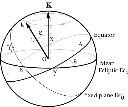
Figure 1: Andoyer’s canonical variables. $L$ is the projection of the total rotational angular momentum vector $\boldsymbol{L}$ on the principal axis of inertia $\boldsymbol{\mathrm{k}}$ and $X$ its projection on the normal to the ecliptic $\boldsymbol{\mathrm{K}}$. The angle between the equinox of date $\gamma$ and a fixed point of the equator $A$ is the hour angle $\theta$, and $\psi=\gamma$ N + N $\gamma_{0}$ is the general precession angle. The direction of $\gamma_{0}$ is on a fixed plane ${E_{c}}_{0}$, while $\gamma$ is on the mean orbital (or ecliptic) ${E_{c}}_{t}$ of date $t$.

2.1 Gravitational potential

The gravitational potential ${\cal V}$ generated by the planet at a generic point of the space $\boldsymbol{r}$ is given by (e.g. Tisserand, 1891; Smart, 1953):

$${\cal V}(\boldsymbol{r})=-{{\displaystyle Gm}\over{\displaystyle r}} + {{\displaystyle G(B-A)}\over{\displaystyle r^{3}}}P_{2}(\boldsymbol{\hat{r}}\cdot\boldsymbol{\mathrm{j}})$$ (1)

$$+ {{\displaystyle G(C-A)}\over{\displaystyle r^{3}}}P_{2}(\boldsymbol{\hat{r}}\cdot\boldsymbol{\mathrm{k}})\ ,$$ (2)

where $G$ is the gravitational constant, $\boldsymbol{\hat{r}}=\boldsymbol{r}/r$ and $P_{2}(x)=(3x^{2}-1)/2$ are the Legendre polynomials of degree two. The potential energy ${\cal U}$ when orbiting a central star of mass $m_{\odot}$ is then:

$${\cal U}=m_{\odot}{\cal V}(\boldsymbol{r})\ .$$ (3)

For a planet evolving in a non-perturbed keplerian orbit, we write:

$$\boldsymbol{\hat{r}}=\cos(\varpi+v)\boldsymbol{\mathrm{I}}+\sin(\varpi+v)\boldsymbol{\mathrm{J}}\ ,$$ (4)

where $\varpi$ is the longitude of the perihelion and $v$ the true anomaly. Thus, transforming the body equatorial frame $(\boldsymbol{\mathrm{i}},\boldsymbol{\mathrm{j}},\boldsymbol{\mathrm{k}})$ in the ecliptic one $(\boldsymbol{\mathrm{I}},\boldsymbol{\mathrm{J}},\boldsymbol{\mathrm{K}})$, we obtain (e.g. Correia, 2006):

$$\left\{\begin{array}[]{l l}\boldsymbol{\hat{r}}\cdot\boldsymbol{\mathrm{j}}=-\cos w\sin\theta+\sin w\cos\theta\cos\varepsilon\ ,\cr\vskip 6.0pt plus 2.0pt minus 2.0pt\cr\boldsymbol{\hat{r}}\cdot\boldsymbol{\mathrm{k}}=-\sin w\sin\varepsilon\ ,\end{array}\right.$$ (5)

where $w=\varpi+\psi+v$ is the true longitude of date. The expression for the potential energy (3) becomes:

$${\cal U} = -{{\displaystyle Gmm_{\odot}}\over{\displaystyle r}}+{{\displaystyle GCm_{\odot}}\over{\displaystyle r^{3}}}E_{d}P_{2}(\sin w\sin\varepsilon)$$ (7)

$$-{{\displaystyle 3Gm_{\odot}}\over{\displaystyle 8r^{3}}}(B-A)\,F(\theta,w,\varepsilon)\ ,$$

where

$$F(\theta,w,\varepsilon)=2\cos(2\theta-2w)\cos^{4}\left({{\displaystyle\varepsilon}\over{\displaystyle 2}}\right)\quad\quad\quad\quad\quad$$ (8)

$$+2\cos(2\theta+2w)\sin^{4}\left({{\displaystyle\varepsilon}\over{\displaystyle 2}}\right)+\cos(2\theta)\sin^{2}\varepsilon$$ (9)

and

$$E_{d}=\frac{C-\frac{1}{2}(A+B)}{C}=\frac{k_{f}R^{5}}{3GC}\omega^{2}+\delta E_{d}\ .$$ (10)

$R$ is the planet’s radius and $k_{f}$ the fluid Love number (pertaining to a perfectly fluid body with the same mass distribution as the actual planet). $E_{d}$ is the dynamical ellipticity, the first part of this expression corresponding to the flattening in hydrostatic equilibrium (Lambeck, 1980), and $\delta E_{d}$ to the departure from this equilibrium.

2.2 Averaged potential

Since we are only interested in the study of the long-term motion, we will average the potential energy ${\cal U}$ over the rotation angle $\theta$ and the mean anomaly $M$, after expanding the true anomaly $v$ in series of the eccentricity $e$ and mean anomaly. However, when the rotation frequency $\omega\simeq\dot{\theta}$ and the mean motion $n=\dot{M}$ are close to resonance ($\omega\simeq pn$, for a semi-integer value $p$), we must retain the terms with argument $2(\theta-pM)$ in the expansions

$$\frac{\cos(2\theta)}{r^{3}}=\frac{1}{a^{3}}\sum^{+\infty}_{p=-\infty}G(p,e)\cos(2\theta-2pM)$$ (11)

and

$$\frac{\cos(2\theta-2v)}{r^{3}}=\frac{1}{a^{3}}\sum^{+\infty}_{p=-\infty}H(p,e)\cos(2\theta-2pM)\ ,$$ (12)

where $a$ is the semi-major axis of the planet’s orbit and the functions $G(p,e)$ and $H(p,e)$ are power series in $e$ (Tab. 1).

$\quad p\quad$			$G(p,e)$					$H(p,e)$
$\hbox to0.0pt{\hss$-$}1$			${{\displaystyle 9}\over{\displaystyle 4}}e^{2}$	$+$	${{\displaystyle 7}\over{\displaystyle 4}}e^{4}$					${{\displaystyle 1}\over{\displaystyle 24}}e^{4}$
$\hbox to0.0pt{\hss$-$}1/2$		${{\displaystyle 3}\over{\displaystyle 2}}e$	$+$	${{\displaystyle 27}\over{\displaystyle 16}}e^{3}$					${{\displaystyle 1}\over{\displaystyle 48}}e^{3}$
$0$	$1$	$+$	${{\displaystyle 3}\over{\displaystyle 2}}e^{2}$	$+$	${{\displaystyle 15}\over{\displaystyle 8}}e^{4}$	$0$
$1/2$		${{\displaystyle 3}\over{\displaystyle 2}}e$	$+$	${{\displaystyle 27}\over{\displaystyle 16}}e^{3}$		$-$	${{\displaystyle 1}\over{\displaystyle 2}}e$	$+$	${{\displaystyle 1}\over{\displaystyle 16}}e^{3}$
$1$			${{\displaystyle 9}\over{\displaystyle 4}}e^{2}$	$+$	${{\displaystyle 7}\over{\displaystyle 4}}e^{4}$	$1$	$-$	${{\displaystyle 5}\over{\displaystyle 2}}e^{2}$	$+$	${{\displaystyle 13}\over{\displaystyle 16}}e^{4}$
$3/2$				${{\displaystyle 53}\over{\displaystyle 16}}e^{3}$			${{\displaystyle 7}\over{\displaystyle 2}}e$	$-$	${{\displaystyle 123}\over{\displaystyle 16}}e^{3}$
$2$					${{\displaystyle 77}\over{\displaystyle 16}}e^{4}$			${{\displaystyle 17}\over{\displaystyle 2}}e^{2}$	$-$	${{\displaystyle 115}\over{\displaystyle 6}}e^{4}$
$5/2$									${{\displaystyle 845}\over{\displaystyle 48}}e^{3}$
$3$										${{\displaystyle 533}\over{\displaystyle 16}}e^{4}$

Table 1: Coefficients of $G(p,e)$ and $H(p,e)$ to $e^{4}$. The exact expression of these coefficients is given by $G(p,e)=\frac{1}{\pi}\int_{0}^{\pi}\left(\frac{a}{r}\right)^{3}\exp(\mathrm{i}\,2pM)\,dM$ and $H(p,e)=\frac{1}{\pi}\int_{0}^{\pi}\left(\frac{a}{r}\right)^{3}\exp(\mathrm{i}\,2\nu)\exp(\mathrm{i}\,2pM)\,dM$.

The averaged potential $\overline{\cal U}$ becomes:

$${{\displaystyle\overline{\cal U}}\over{\displaystyle C}} = -\alpha{{\displaystyle\omega\,x^{2}}\over{\displaystyle 2}}-{{\displaystyle\beta}\over{\displaystyle 4}}\left[(1-x^{2})\,G(p,e)\cos 2(\theta-pM)\phantom{{{\displaystyle.}\over{\displaystyle.}}}\right.$$ (15)

$$+{{\displaystyle(1+x)^{2}}\over{\displaystyle 2}}\,H(p,e)\cos 2(\theta-pM-\phi)$$

$$+\left.{{\displaystyle(1-x)^{2}}\over{\displaystyle 2}}\,H(-p,e)\cos 2(\theta-pM+\phi)\right]\ ,$$

where $x=X/L=\cos\varepsilon$, $\phi=\varpi+\psi$,

$$\alpha={{\displaystyle 3Gm_{\odot}}\over{\displaystyle 2a^{3}(1-e^{2})^{3/2}}}{{\displaystyle E_{d}}\over{\displaystyle\omega}}\simeq{{\displaystyle 3}\over{\displaystyle 2}}{{\displaystyle n^{2}}\over{\displaystyle\omega}}(1-e^{2})^{-3/2}E_{d}$$ (16)

is the ‘precession constant’ and

$$\beta={{\displaystyle 3Gm_{\odot}}\over{\displaystyle 2a^{3}}}{{\displaystyle B-A}\over{\displaystyle C}}\simeq{{\displaystyle 3}\over{\displaystyle 2}}n^{2}{{\displaystyle B-A}\over{\displaystyle C}}\ .$$ (17)

We can rewrite expression (15) simplified as:

$${{\displaystyle\overline{\cal U}}\over{\displaystyle C}}=-\alpha{{\displaystyle\omega\,x^{2}}\over{\displaystyle 2}}-{{\displaystyle\beta_{x}}\over{\displaystyle 2}}\cos 2(\theta-pM-\phi_{x})\ ,$$ (18)

where the amplitude $\beta_{x}$ and the phase angle $\phi_{x}$ are functions depending on both $x$ and $\psi$, whose expressions are given in appendix A.

2.3 Equations of motion

The Andoyer variables ($L$, $\theta$) and ($X$, $-\psi$) are canonically conjugated and thus

$$\frac{dL}{dt}=-\frac{\partial\overline{\cal U}}{\partial\theta}\ ;\quad\frac{dX}{dt}=\frac{\partial\overline{\cal U}}{\partial\psi}\ ;\quad\frac{d\psi}{dt}=-\frac{\partial\overline{\cal U}}{\partial X}\ .$$ (19)

Despite their practical use, Andoyer’s variables do not give a clear view of the obliquity variations. Since $\cos\varepsilon=X/L$ they can be obtained as:

$$\sin\varepsilon\,\frac{d\varepsilon}{dt}=\frac{1}{L}\left(\frac{X}{L}\frac{dL}{dt}-\frac{dX}{dt}\right)=-\frac{1}{L}\left[x\frac{\partial\overline{\cal U}}{\partial\theta}+\frac{\partial\overline{\cal U}}{\partial\psi}\right]\ .$$ (20)

Then, from equation (15) we get:

$$\frac{dL}{dt}=-C\beta_{x}\sin 2(\theta-pM-\phi_{x})\ ,$$ (21)

$$\frac{d\varepsilon}{dt}=-\alpha_{r}\sin\varepsilon\cos 2(\theta-pM-\phi_{r})\ ,$$ (22)

and

$$\frac{d\psi}{dt}=\alpha\,x+\alpha_{r}\sin 2(\theta-pM-\phi_{r})\ ,$$ (23)

where $\alpha_{r}$ and $\phi_{r}$ are functions depending on both $x$ and $\psi$, whose expressions are given in appendix A. For non-resonant motion the previous equations simplify as:

$$\frac{dL}{dt}=\frac{d\varepsilon}{dt}=0\quad\mathrm{and}\quad\frac{d\psi}{dt}=\alpha\cos\varepsilon\ .$$ (24)

The planet spin motion reduces to the precession of the spin vector about the normal to the orbital plane with rate $\alpha\cos\varepsilon$. In general we have $\alpha\gg\alpha_{r}$ and the precession rate including the resonant motion (Eq.23) is nearly the same as the non-resonant case (Eq.24).

3 Tidal effects

Tidal effects arise from differential and inelastic deformations of the planet due to the gravitational effect of a perturbing body. Their contributions to the spin variations are based on a very general formulation of the tidal potential, initiated by George H. Darwin (1880). The attraction of a body with mass $m_{\odot}$ at a distance $r$ from the center of mass of the planet can be expressed as the gradient of a scalar potential ${\cal V}^{\prime}$, which is a sum of Legendre polynomials:

$${\cal V}^{\prime}=\sum_{l=2}^{\infty}{\cal V}_{l}^{\prime}=-\frac{Gm_{\odot}}{r}\sum_{l=2}^{\infty}\left(\frac{r^{\prime}}{r}\right)^{l}P_{l}(\cos S)\ ,$$ (25)

where $r^{\prime}$ is the radial distance from the planet’s center, and $S$ the angle between $\boldsymbol{r}$ and $\boldsymbol{r}^{\prime}$. The distortion of the planet by this potential gives rise to a tidal potential,

$${\cal V}^{g}=\sum_{l=2}^{\infty}{\cal V}_{l}^{g}\ ,$$ (26)

where ${\cal V}_{l}^{g}=k_{l}{\cal V}_{l}^{\prime}$ at the planet’s surface and $k_{l}$ is the Love number for potential. Since the tidal potential ${\cal V}_{l}^{g}$ is an $l$th degree harmonic, exterior to the planet it must be proportional to $r^{-l-1}$ (solution of a Dirichlet problem). Furthermore, as upon the surface $r^{\prime}=R\ll r$, we can retain in the expansion only its first term, $l=2$:

$${\cal V}^{g}=-k_{2}\frac{Gm_{\odot}}{R}\left(\frac{R}{r}\right)^{3}\left(\frac{R}{r^{\prime}}\right)^{3}P_{2}(\cos S)\ .$$ (27)

In general, imperfect elasticity will cause the phase angle of ${\cal V}^{g}$ to lag behind that of ${\cal V}^{\prime}$ (Kaula, 1964) by an angle $\delta(\sigma)$ such that:

$$\delta(\sigma)=\frac{\sigma\Delta t(\sigma)}{2}\ ,$$ (28)

$\Delta t(\sigma)$ being the time lag associated to the tidal frequency $\sigma$ (a linear combination of the inertial rotation rate $\omega$ and the mean orbital motion $n$).

3.1 Equations of motion

Expressing the tidal potential given by expression (27) in terms of Andoyer angles $(\theta,\psi)$, we then easily obtain its contribution to the spin evolution as:

$$\frac{dL}{dt}=-m^{\prime}\frac{\partial{\cal V}^{g}}{\partial\theta}\ ;\quad\frac{dX}{dt}=m^{\prime}\frac{\partial{\cal V}^{g}}{\partial\psi}\ ;$$ (29)

where $m^{\prime}$ is the mass of the interacting body. As we are interested here in the study of the secular evolution of the spin, we will average (29) over the periods of mean anomaly, longitude of node and perihelion of the perturbing body. When the interacting body is the same as the perturbing one $(m^{\prime}=m_{\odot})$, we obtain:

$${{\displaystyle dL}\over{\displaystyle dt}}=-{{\displaystyle Gm_{\odot}^{2}R^{5}}\over{\displaystyle a^{6}}}\sum_{\sigma}b(\sigma)\Theta^{L}_{\sigma}(x,e)\ ,$$ (30)

$${{\displaystyle d\varepsilon}\over{\displaystyle dt}}=-{{\displaystyle Gm_{\odot}^{2}R^{5}}\over{\displaystyle a^{6}}}{{\displaystyle\sin\varepsilon}\over{\displaystyle L}}\sum_{\sigma}b(\sigma)\Theta^{\varepsilon}_{\sigma}(x,e)\ ,$$ (31)

where the coefficients $\Theta_{\sigma}(x,e)$ are polynomials in the eccentricity (Kaula, 1964). The factors $b(\sigma)$ are related to the dissipation of the mechanical energy of tides in the planet’s interior responsible for the time delay $\Delta t(\sigma)$ between the position of “maximal tide” and the sub-solar point. They are related to the phase lag $\delta(\sigma)$ as:

$$b(\sigma)=k_{2}\sin 2\delta(\sigma)=k_{2}\sin\left(\sigma\Delta t(\sigma)\right)\ .$$ (32)

Dissipation equations (30) and (31) must be invariant under the change $(\omega,\varepsilon)$ by $(-\omega,\pi-\varepsilon)$ which imposes that $b(\sigma)=-b(-\sigma)$, that is, $b(\sigma)$ is an odd function of $\sigma$. Although mathematically equivalent, the couples $(\omega,\varepsilon)$ and $(-\omega,\pi-\varepsilon)$ correspond to two different physical situations (Correia and Laskar, 2001).

3.2 Dissipation models

The dissipation of the mechanical energy of tides in the planet’s interior is responsible for the phase lags $\delta(\sigma)$. A commonly used dimensionless measure of tidal damping is the quality factor $Q$ (Munk and MacDonald, 1960), defined as the inverse of the “specific” dissipation and related to the phase lags by

$$Q(\sigma)=\frac{2\pi E}{\Delta E}=\cot 2\delta(\sigma)\ ,$$ (33)

where $E$ is the total tidal energy stored in the planet, and $\Delta E$ the energy dissipated per cycle. We can rewrite (32) as:

$$b(\sigma)=\frac{k_{2}\,\mathrm{sign}(\sigma)}{\sqrt{Q^{2}(\sigma)+1}}\simeq\mathrm{sign}(\sigma)\frac{k_{2}}{Q(\sigma)}\ .$$ (34)

The present $Q$ value of the planets in the Solar system can be estimated from orbital measurements, but as rheology of the planets is badly known, the dependence of $b(\sigma)$ on the tidal frequency $\sigma$ is subject to various approximations.

3.2.1 The visco-elastic model

Darwin (1908) assumed that the planet behaves like a Maxwell solid of constant density $\rho$, and found:

$$b(\sigma)=k_{f}\frac{\tau_{b}-\tau_{a}}{1+(\tau_{b}\,\sigma)^{2}}\sigma\ ,$$ (35)

where $\tau_{a}=\upsilon_{e}/\mu_{e}$ and $\tau_{b}$ are the time constants for damping of the body tides,

$$\tau_{b}=\tau_{a}(1+19\mu_{e}R/2Gm\rho)\ .$$ (36)

The visco-elastic model is a very realistic approximation of the planet’s deformation with the tidal frequency. However, when replacing expression (35) into the dynamical equations (30) and (31) we get an infinite sum of terms. This problem can be solved by using simplified versions of the visco-elastic model for specific values of the tidal frequency $\sigma$. For instance, when $\sigma$ is small, $(\tau_{b}\,\sigma)^{2}$ can be neglected in (35) and $b(\sigma)$ becomes proportional to $\sigma$.

3.2.2 The viscous or linear model

In this model, it is assumed that the response time delay to the perturbation is independent of the tidal frequency, i.e., the position of the “maximal tide” is shifted from the sub-solar point by a constant time lag $\Delta t$ (Mignard, 1979, 1980). As usually we have $\sigma\Delta t\ll 1$, this model becomes linear:

$$b^{g}(\sigma)=k_{2}\sin(\sigma\Delta t)\simeq k_{2}\,\sigma\Delta t\ .$$ (37)

Substituting the above formula into expressions (30) and (31), we simplify the motion equations as (appendix B):

$$\left\{\begin{array}[]{l l}{{\displaystyle dL}\over{\displaystyle dt}}=-CK\left[{{\displaystyle 1+x^{2}}\over{\displaystyle 2}}\,\Omega(e){{\displaystyle\omega}\over{\displaystyle n}}-xN(e)\right]\ ,\cr\vskip 6.0pt plus 2.0pt minus 2.0pt\cr{{\displaystyle d\varepsilon}\over{\displaystyle dt}}=K{{\displaystyle\sin\varepsilon}\over{\displaystyle\omega}}\left[x\,\Omega(e){{\displaystyle\omega}\over{\displaystyle 2n}}-N(e)\right]\ ,\end{array}\right.$$ (38)

where

$$\Omega(e)={{\displaystyle 1+3e^{2}+3e^{4}/8}\over{\displaystyle(1-e^{2})^{9/2}}}\ ,$$ (39)

$$N(e)={{\displaystyle 1+15e^{2}/2+45e^{4}/8+5e^{6}/16}\over{\displaystyle(1-e^{2})^{6}}}\ ,$$ (40)

$$K=n^{2}\,\frac{3\,k_{2}}{\xi\,Q}\left(\frac{m_{\odot}}{m}\right)\left(\frac{R}{a}\right)^{3}\ ,$$ (41)

$Q^{-1}=n\Delta t$ and $\xi=C/(mR^{2})$. The viscous model is a particular case of the visco-elastic model and is specially adapted to describe the behavior of planets in slow rotating regimes ($\omega\sim n$).

3.2.3 The constant-$Q$ model

Since for the Earth, $Q$ changes by less than an order of magnitude between the Chandler wobble period (about 440 days) and seismic periods of a few seconds, it is also common to treat the specific dissipation as independent of frequency. Thus,

$$b^{g}(\sigma)\simeq\mathrm{sign}(\sigma)k_{2}/Q\ .$$ (42)

For long-term evolutions and slow rotating planets, this model is not appropriate as it gives rise to discontinuities for $\sigma=0$. However, it can be used for periods of time where the tidal frequency does not change much, as is the case for fast rotating planets. Substituting Eq.(42) into expressions (30) and (31), we can simplify the motion equations as:

$$\left\{\begin{array}[]{l l}{{\displaystyle dL}\over{\displaystyle dt}}=-s_{g}{{\displaystyle CK}\over{\displaystyle 16}}\left(5+6x^{2}-3x^{4}\right)\Omega(e)\ ,\cr\vskip 6.0pt plus 2.0pt minus 2.0pt\cr{{\displaystyle d\varepsilon}\over{\displaystyle dt}}={{\displaystyle K}\over{\displaystyle 16}}\,{{\displaystyle\sin\varepsilon}\over{\displaystyle\omega}}\left(3-7s_{g}\,x-3x^{2}+3s_{g}\,x^{3}\right)\Omega(e)\ ,\end{array}\right.$$ (43)

where $s_{g}=\mathrm{sign}(L)=\mathrm{sign}(\omega)$.

4 Core-mantle friction effect

The Mariner 10 flyby of Mercury revealed the presence of an intrinsic magnetic field, which is most likely due to motions in a conducting fluid inner core (for a review see Ness, 1978; Spohn et al., 2001). Subsequent observations made with Earth-based radar provided strong evidence that the mantle of Mercury is decoupled from a core that is at least partially molten (Margot et al., 2007). If there is slippage between the liquid core and the mantle, a second source of dissipation of rotational energy results from friction occurring at the core-mantle boundary. Indeed, because of their different shapes and densities, the core and the mantle do not have the same dynamical ellipticity and the two parts tend to precess at different rates (Poincaré, 1910). This tendency is more or less counteracted by different interactions produced at their interface: the torque $\boldsymbol{N}$ of non-radial inertial pressure forces of the mantle over the core provoked by the non-spherical shape of the interface; the torque of the viscous (or turbulent) friction between the core and the mantle; the torque of the electromagnetic friction, caused by the interaction between electrical currents of the core and the bottom of the magnetized mantle.

4.1 Equations of motion

We will adopt henceforward a model for the planet which is an extension of the model from Poincaré (1910) of a perfect incompressible and homogeneous liquid core with moments of inertia $A_{c}=B_{c}<C_{c}$ inside an homogeneous rigid body with moments of inertia $A_{m}\leq B_{m}<C_{m}$, supported by the same reference frame $(\boldsymbol{\mathrm{i}},\boldsymbol{\mathrm{j}},\boldsymbol{\mathrm{k}})$, fixed with respect to the planet’s figure (Fig.1). The combined effects of inertial and frictional coupling across the ellipsoidal core-mantle boundary are taken into account, assuming laminar flow.

Denoting $\boldsymbol{\delta}=\boldsymbol{\omega}-\boldsymbol{\omega}_{c}$ the differential rotation between the core and the mantle, we can write the non-radial inertial pressure torque of the mantle on the core in a general formulation to first order in the core dynamical ellipticity, $E_{c}$, as (Rochester, 1976; Sasao et al., 1980; Pais et al., 1999):

$$\boldsymbol{N}=\boldsymbol{\omega}_{c}\times\boldsymbol{L}_{c}=C_{c}E_{c}\,\omega\,\boldsymbol{\mathrm{k}}\times\boldsymbol{\delta}\ ,$$ (44)

where $\boldsymbol{L}_{c}=\tilde{\cal I}_{c}\cdot\boldsymbol{\omega}_{c}$ is the core angular momentum with $\tilde{\cal I}_{c}=\mathrm{diag}(A_{c},A_{c},C_{c})$ its tensor of inertia.

The two types of friction torques (viscous and electromagnetic) depend on the differential rotation between the core and the mantle and can be expressed by a single effective friction torque, $\boldsymbol{\Gamma}$. As a general expression for this torque we adopt (Rochester, 1976; Sasao et al., 1980; Mathews and Guo, 2005)

$$\boldsymbol{\Gamma}=C_{c}\,(\kappa+\kappa^{\prime}\,\boldsymbol{\mathrm{k}}\times)\,\boldsymbol{\delta}\ ,$$ (45)

where $\kappa$ and $\kappa^{\prime}$ are effective coupling parameters. They result either from viscous and electromagnetic stresses at the core-mantle interface and can be written as a sum of these two effects: $\kappa=\kappa_{\mathrm{vis}}+\kappa_{\mathrm{em}}$ and $\kappa^{\prime}=\kappa_{\mathrm{vis}}^{\prime}+\kappa_{\mathrm{em}}^{\prime}$. Recent estimations of these coefficients can be found in the works of Mathews and Guo (2005) and Deleplace and Cardin (2006). In the simplified case of no magnetic field, the coupling parameters are only given by the viscous friction contributions, which can be simplified as (Noir et al., 2003; Mathews and Guo, 2005):

$$\kappa_{\mathrm{vis}}=2.62\sqrt{\nu\arrowvert\omega\arrowvert}/R_{c}\quad\mathrm{and}\quad\kappa_{\mathrm{vis}}^{\prime}=0.259\sqrt{\nu\arrowvert\omega\arrowvert}/R_{c}\ ,$$ (46)

where $R_{c}$ is the core radius and $\nu$ the kinematic viscosity, which is poorly known. Even in the case of the Earth, the uncertainty in $\nu$ covers about 13 orders of magnitude (Lumb and Aldridge, 1991), the best estimate so far being $\nu\simeq 10^{-6}\,\mathrm{m}^{2}\mathrm{s}^{-1}$ (Gans, 1972; Poirier, 1988; Wijs et al., 1998).

Since the derivative of the angular momentum is given by the sum of external torques, the contribution of the core-mantle friction is the solution of the system:

$$\left\{\begin{array}[]{l l}{{\displaystyle d\boldsymbol{L}_{m}}\over{\displaystyle dt}}=\boldsymbol{P}+\boldsymbol{T}-\boldsymbol{N}-\boldsymbol{\Gamma}\ ,\cr\vskip 6.0pt plus 2.0pt minus 2.0pt\cr{{\displaystyle d\boldsymbol{L}_{c}}\over{\displaystyle dt}}=\boldsymbol{N}+\boldsymbol{\Gamma}\ ,\end{array}\right.$$ (47)

where $\boldsymbol{P}=\boldsymbol{r}\times\nabla{\cal U}$ is the precession torque and $\boldsymbol{T}=\boldsymbol{r}\times m^{\prime}\nabla{\cal V}^{g}$ the tidal torque. $\boldsymbol{L}_{m}$ denotes the mantle’s angular momentum,

$$\boldsymbol{L}_{m}=C_{m}\,\boldsymbol{\omega}=C_{m}\,\omega\,\boldsymbol{\mathrm{k}}$$ (48)

and the total angular momentum variations are given by:

$${{\displaystyle d\boldsymbol{L}}\over{\displaystyle dt}}={{\displaystyle d\boldsymbol{L}_{m}}\over{\displaystyle dt}}+{{\displaystyle d\boldsymbol{L}_{c}}\over{\displaystyle dt}}=\boldsymbol{P}+\boldsymbol{T}\ .$$ (49)

$\boldsymbol{L}$ precesses around $\boldsymbol{\mathrm{K}}$, a normal vector to the orbital plane, with angular velocity $\boldsymbol{\Omega}$ given by:

$$\boldsymbol{\Omega}=-\dot{\psi}\boldsymbol{\mathrm{K}}+\dot{\varepsilon}\,\boldsymbol{p}\ ,$$ (50)

where $\dot{\varepsilon}$ accounts for the secular effects resulting from tides and core-mantle friction and $\boldsymbol{p}\equiv\boldsymbol{\mathrm{K}}\times\boldsymbol{\mathrm{k}}\,/\sin\varepsilon$ is the unit vector along the direction of the averaged precession. Thus,

$${{\displaystyle d\boldsymbol{L}}\over{\displaystyle dt}}=\boldsymbol{\Omega}\times\boldsymbol{L}=\boldsymbol{\Omega}\times\left(C\omega\boldsymbol{\mathrm{k}}-\tilde{\cal I}_{c}\cdot\boldsymbol{\delta}\right)\ .$$ (51)

Projecting it over

$$\boldsymbol{q}\equiv\boldsymbol{\mathrm{k}}\times\boldsymbol{p}=\frac{\boldsymbol{\mathrm{K}}-\boldsymbol{\mathrm{k}}\cos\varepsilon}{\sin\varepsilon}\ ,$$ (52)

we get

$$(\boldsymbol{\Omega}\times\boldsymbol{L})\!\!\! \cdot \!\!\!(\boldsymbol{\mathrm{k}}\times\boldsymbol{p})\ \ =\ \ (\boldsymbol{\Omega}\cdot\boldsymbol{\mathrm{k}})(\boldsymbol{L}\cdot\boldsymbol{p})-(\boldsymbol{\Omega}\cdot\boldsymbol{p})(\boldsymbol{L}\cdot\boldsymbol{\mathrm{k}})$$ (53)

$$= -\dot{\psi}\cos\varepsilon\,(-\boldsymbol{p}\cdot\tilde{\cal I}_{c}\cdot\boldsymbol{\delta})-\dot{\varepsilon}\,(C\omega-\boldsymbol{\mathrm{k}}\cdot\tilde{\cal I}_{c}\cdot\boldsymbol{\delta})$$ (54)

$$= \dot{\psi}\cos\varepsilon A_{c}\delta_{p}-\dot{\varepsilon}(C\omega-C_{c}\delta_{k})\ ,$$ (55)

with $\delta_{\mathrm{k}}=\boldsymbol{\delta}\cdot\boldsymbol{\mathrm{k}}$ and $\delta_{p}=\boldsymbol{\delta}\cdot\boldsymbol{p}$. Then, assuming $\delta_{k}\ll\omega$ we have from expression (49)

$$\dot{\varepsilon}=-{{\displaystyle P_{q}}\over{\displaystyle C\omega}}-{{\displaystyle T_{q}}\over{\displaystyle C\omega}}+{{\displaystyle\dot{\psi}\cos\varepsilon A_{c}\delta_{p}}\over{\displaystyle C\omega}}\ ,$$ (56)

where $-P_{q}/C\omega$ and $-T_{q}/C\omega$ are respectively given by expressions (22) and (31). The value of $\delta_{p}$ in the case of uniform precession is (Rochester, 1976; Pais et al., 1999; Correia, 2006):

$$\delta_{p}={{\displaystyle-\kappa\,\omega\,\dot{\psi}\sin\varepsilon}\over{\displaystyle\kappa^{2}+(\kappa^{\prime}+E_{c}\omega)^{2}}}\ .$$ (57)

In the case of a non-uniform precession, as it can be the case of Mercury close to a spin-orbit resonance, Correia (2006) shows that the asymmetric terms in $(B-A)$ are periodic and average to zero, and we can still use the previous expression for $\delta_{p}$. Using $c_{c}=C_{c}/C$, $A_{c}\simeq C_{c}$ and $\dot{\psi}\simeq\alpha\cos\varepsilon$, we finally have for the obliquity variations with core-mantle friction:

$$\dot{\varepsilon}=-{{\displaystyle P_{q}}\over{\displaystyle C\omega}}-{{\displaystyle T_{q}}\over{\displaystyle C\omega}}-K_{f}\cos^{3}\varepsilon\sin\varepsilon\ ,$$ (58)

with

$$K_{f}={{\displaystyle c_{c}\kappa\,\alpha^{2}}\over{\displaystyle\kappa^{2}+(\kappa^{\prime}+E_{c}\omega)^{2}}}\ ,$$ (59)

which is always a positive quantity.

The rotation rate variations of the mantle and the core can be obtained by projecting both equations (47) onto $\boldsymbol{\mathrm{k}}$:

$${{\displaystyle d}\over{\displaystyle dt}}(\boldsymbol{L}_{i}\cdot\boldsymbol{\mathrm{k}})={{\displaystyle d\boldsymbol{L}_{i}}\over{\displaystyle dt}}\cdot\boldsymbol{\mathrm{k}}+\boldsymbol{L}_{i}\cdot{{\displaystyle d\boldsymbol{\mathrm{k}}}\over{\displaystyle dt}}={{\displaystyle d\boldsymbol{L}_{i}}\over{\displaystyle dt}}\cdot\boldsymbol{\mathrm{k}}+\boldsymbol{L}_{i}\cdot(\boldsymbol{\Omega}\times\boldsymbol{\mathrm{k}})\ .$$ (60)

For the mantle, $\boldsymbol{L}_{i}$ is given by expression (48) and then

$$C_{m}{{\displaystyle d\omega}\over{\displaystyle dt}}=P_{\mathrm{k}}+T_{\mathrm{k}}-C_{c}\kappa\,\delta_{\mathrm{k}}\ ,$$ (61)

where $P_{\mathrm{k}}$ and $T_{\mathrm{k}}$ are respectively given by expressions (21) and (30). For the core $\boldsymbol{L}_{i}=\boldsymbol{L}_{c}=\tilde{\cal I}_{c}\cdot\boldsymbol{\omega}_{c}$ and we have

$$C_{c}{{\displaystyle d\omega_{c}^{\mathrm{k}}}\over{\displaystyle dt}} = C_{c}\kappa\,\delta_{\mathrm{k}}+\boldsymbol{L}_{c}\cdot(-\dot{\psi}\sin\varepsilon\,\boldsymbol{p}-\dot{\varepsilon}\,\boldsymbol{q})$$ (62)

$$= C_{c}\kappa\,\delta_{\mathrm{k}}+A_{c}\dot{\psi}\sin\varepsilon\,\delta_{p}+A_{c}\dot{\varepsilon}\,\delta_{q}\ ,$$ (63)

where $\omega_{c}^{\mathrm{k}}=\boldsymbol{\omega}_{c}\cdot\boldsymbol{\mathrm{k}}=\omega-\delta_{\mathrm{k}}$ and $\delta_{p}$ is given by expression (57). We can also neglect the term in $A_{c}\,\dot{\varepsilon}\,\delta_{q}$ because according to expression (56) its average is a second order term in $\delta$. Thus, using $A_{c}\simeq C_{c}$ we have

$${{\displaystyle d\omega_{c}^{\mathrm{k}}}\over{\displaystyle dt}}=\kappa\,\delta_{\mathrm{k}}-{{\displaystyle\omega K_{f}}\over{\displaystyle c_{c}}}\cos^{2}\varepsilon\sin^{2}\varepsilon\ .$$ (64)

4.2 Differential rotation

Combining equations (61) and (63) we find a differential equation for $\delta_{\mathrm{k}}$,

$${{\displaystyle d\delta_{\mathrm{k}}}\over{\displaystyle dt}}=-\kappa_{m}\,\delta_{\mathrm{k}}+{{\displaystyle P_{\mathrm{k}}}\over{\displaystyle C_{m}}}+{{\displaystyle T_{\mathrm{k}}}\over{\displaystyle C_{m}}}-{{\displaystyle A_{c}}\over{\displaystyle C_{c}}}\dot{\psi}\sin\varepsilon\,\delta_{p}\ ,$$ (65)

where $\kappa_{m}=\kappa\,C/C_{m}$. Its solution allows us completely to determine the spin of the mantle (Eq.61) without needing the core variations (Eq.63):

$$\delta_{\mathrm{k}}(t)=\mathrm{e}^{-\kappa_{m}t}\int\left({{\displaystyle P_{\mathrm{k}}}\over{\displaystyle C_{m}}}+{{\displaystyle T_{\mathrm{k}}}\over{\displaystyle C_{m}}}-{{\displaystyle A_{c}}\over{\displaystyle C_{c}}}\dot{\psi}\sin\varepsilon\,\delta_{p}\right)\mathrm{e}^{\kappa_{m}t}dt\ .$$ (66)

The secular variations to the spin can be seen as constant for short-periods of time. Thus, since among all the contributions inside the integral of previous expression only $P_{\mathrm{k}}$ is not secular, we have

$$\delta_{\mathrm{k}}(t)={{\displaystyle 1}\over{\displaystyle\kappa}}\left({{\displaystyle T_{\mathrm{k}}}\over{\displaystyle C}}-{{\displaystyle C_{m}}\over{\displaystyle C}}\dot{\psi}\sin\varepsilon\,\delta_{p}\right)+P(t)\ ,$$ (67)

with

$$P(t)=\mathrm{e}^{-\kappa_{m}t}\int{{\displaystyle P_{\mathrm{k}}}\over{\displaystyle C_{m}}}\,\mathrm{e}^{\kappa_{m}t}dt\ .$$ (68)

4.2.1 Strong coupling

We consider a strong coupling between the core and the mantle whenever $\kappa^{2}\gg\beta$, where $\beta$ is given by expression (17). In this case, we can simplify expression (68) by performing an integration by parts:

$$P(t)={{\displaystyle 1}\over{\displaystyle\kappa}}{{\displaystyle P_{\mathrm{k}}}\over{\displaystyle C}}-{{\displaystyle 1}\over{\displaystyle\kappa^{2}}}{{\displaystyle C_{m}}\over{\displaystyle C^{2}}}{{\displaystyle\partial P_{\mathrm{k}}}\over{\displaystyle\partial t}}\ ,$$ (69)

where we neglected terms higher than $\beta/\kappa^{2}$. Substituting the above equation (69) into expression (61) we find for the rotation rate variations:

$${{\displaystyle d\omega}\over{\displaystyle dt}}={{\displaystyle P_{\mathrm{k}}}\over{\displaystyle C}}+{{\displaystyle T_{\mathrm{k}}}\over{\displaystyle C}}-\omega K_{f}\cos^{2}\varepsilon\sin^{2}\varepsilon+{{\displaystyle c_{c}}\over{\displaystyle\kappa}}{{\displaystyle\partial}\over{\displaystyle\partial t}}{{\displaystyle P_{\mathrm{k}}}\over{\displaystyle C}}\ .$$ (70)

4.2.2 Weak coupling

For weak coupling we assume $\kappa^{2}\ll\beta$, we will thus neglect second order terms in $\kappa^{2}/\beta$. Performing again an integration by parts in expression (68), but changing the roles of $P_{\mathrm{k}}/C_{m}$ and $\mathrm{e}^{\kappa_{m}t}$ we have:

$$P(t)=\int{{\displaystyle P_{\mathrm{k}}}\over{\displaystyle C_{m}}}\ dt\ ,$$ (71)

which gives for the rotation rate variations when substituted into expression (61):

$${{\displaystyle d\omega}\over{\displaystyle dt}}={{\displaystyle P_{\mathrm{k}}}\over{\displaystyle C_{m}}}+{{\displaystyle T_{\mathrm{k}}}\over{\displaystyle C}}-\omega K_{f}\cos^{2}\varepsilon\sin^{2}\varepsilon-c_{c}\kappa_{m}\int{{\displaystyle P_{\mathrm{k}}}\over{\displaystyle C_{m}}}\ dt\ .$$ (72)

5 Spin-orbit resonances

The resonant equilibrium was first observed in the Moon, that is locked in a 1/1 spin-orbit resonance (e.g. Goldreich, 1966). That other spin-orbit resonances were possible was not realized before the discovery of the 3/2 spin-orbit resonance of Mercury (Pettengill and Dyce, 1965), giving rise to several detailed studies (Colombo, 1965; Colombo and Shapiro, 1966; Goldreich and Peale, 1966; Counselman and Shapiro, 1970). Such non-synchronous spin-orbit resonances require a large orbital eccentricity, but also, as we will see, low obliquity.

5.1 Effect on the rotation rate

Neglecting by now the dissipative effects resulting from tides and core-mantle friction, when combining expressions (21) and (48), we can write near a generic spin-orbit resonance $(\omega\simeq pn)$:

$$\frac{d\omega}{dt}=-\beta_{m}\sin 2(\theta-pM-\phi_{x})\ ,$$ (73)

with $\beta_{m}=\beta_{x}/c_{m}$, where $\beta_{x}$ and $\phi_{x}$ are given in appendix A, and $c_{m}=C_{m}/C$. Let us denote $\gamma=\theta-pM-\phi_{x}$. Since $\omega=\dot{\theta}-\dot{\psi}\cos\varepsilon$ we have $\dot{\gamma}=\omega-pn-\dot{\psi}_{x}$, with $\dot{\psi}_{x}=\dot{\phi}_{x}+\dot{\psi}\cos\varepsilon$. Because we assume $\dot{\psi}\simeq\alpha\cos\varepsilon$ (Eq.24), for small variations of $\omega$ and $\varepsilon$, we can consider $\beta_{x}$, $\dot{\phi}_{x}$ and $\dot{\psi}_{x}$ as constants. Thus, we have $\ddot{\gamma}=\dot{\omega}$ and expression (73) can then be rewritten as

$$\ddot{\gamma}+\beta_{m}\sin 2\gamma=0\ ,$$ (74)

which is the same as the equation of a free pendulum (Fig.2). The first integral of this equation is given by

$$h=\dot{\gamma}^{2}-\beta_{m}\cos 2\gamma\ ,$$ (75)

where $h$ is a constant of the motion related to the energy. The separatrix equation is given by $h=\beta_{m}$, where $h>\beta_{m}$ gives the trajectories in the circulation zone (outside the resonance) and $h<\beta_{m}$ the trajectories in the libration zone (captured in resonance). The maximal and minimal libration width, $\omega_{-}\leq\omega\leq\omega_{+}$, are obtained from the separatrix equation ($h=\beta_{m}$):

$$\omega_{\pm}=pn\pm\Delta\omega\quad\mathrm{with}\quad\Delta\omega=\sqrt{2\beta_{m}}\ ,$$ (76)

Since $\beta_{m}\leq\beta/c_{m}$ (Eq.139), from expression (17) we have:

$$\frac{\Delta\omega}{n}\leq\sqrt{3\frac{B-A}{C_{m}}}\approx 0.02\ ,$$ (77)

using $(B-A)/C_{m}\simeq 1.2\times 10^{-4}$ (Anderson et al., 1987).

5.2 Dissipative torques

Spin-orbit resonant configurations result from an evolutionary process. It is believed that the terrestrial planets’ rotation was faster at the time of their formation, but due to dissipative torques it has decreased (section 6.1) and may have been captured inside a resonance when crossing it.

The secular variations of the rotation rate are easily computed from the mantle’s angular momentum variations (Eqs.61,67) as:

$${{\displaystyle d\omega}\over{\displaystyle dt}}={{\displaystyle P_{\mathrm{k}}}\over{\displaystyle C_{m}}}+\overline{D}\ ,$$ (78)

where

$$\overline{D}={{\displaystyle T_{\mathrm{k}}}\over{\displaystyle C}}-\omega K_{f}(1-x^{2})x^{2}-c_{c}\kappa_{m}P(t)\$$ (79)

denotes the mean dissipative torque ($x=\cos\varepsilon$), which is composed of three terms: the first arising from tidal effects, the second from non-resonant core-mantle friction and the last one is a dissipative term resulting from the presence of spin-orbit resonances and core-mantle friction together.

For the tidal torque we can use the viscous model approximation (section 3.2.2), since significant spin-orbit resonances only occur in the slow rotation regime ($\omega\sim n$). This torque is then given by expression (38), which can be rewritten using $\omega=pn+\dot{\gamma}$ and $E(e)=N(e)/\Omega(e)$ as

$${{\displaystyle T_{\mathrm{k}}}\over{\displaystyle C}}=-K{{\displaystyle 1+x^{2}}\over{\displaystyle 2}}\,\Omega(e)\left[\left(p-{{\displaystyle 2xE(e)}\over{\displaystyle 1+x^{2}}}\right)+{{\displaystyle\dot{\gamma}}\over{\displaystyle n}}\right]\ .$$ (80)

According to expression (77) we have $\dot{\gamma}/n\ll 1$. Thus, the non-resonant core-mantle friction torque can also be made linear:

$$\omega K_{f}(\omega)\simeq pnK_{f}(pn)\left(1+\Omega_{f}{{\displaystyle\dot{\gamma}}\over{\displaystyle n}}\right)\ ,$$ (81)

where

$$\Omega_{f}=n\left[\phantom{\frac{}{}}\!\!\ln(\omega K_{f})\right]^{\prime}_{\omega=pn}=-\frac{q}{p}\ ,$$ (82)

and $q$ is a semi-integer like $p$. Indeed, since $\alpha^{2}\propto\omega^{-2}$ (Eq.16) and $\kappa\propto\omega^{1/2}$ (Eq.46), from expression (59) we have for weak friction ($\kappa\ll E_{c}\omega$) that

$$\omega K_{f}\propto\frac{1}{\omega^{q}}\ ,$$ (83)

with $q=5/2$ and for strong friction ($\kappa\gg E_{c}\omega$) the same previous expression, but $q=3/2$. This result also works for turbulent friction, for which $\kappa\propto 1/\omega$ and thus $q=4$ (Yoder, 1995; Correia et al., 2003).

Finally, for the resonant core-mantle friction contribution we will split our analysis for strong and weak coupling as in section 4.2. In the first situation ($\kappa^{2}\gg\beta$) this calculus is trivial when using expression (73) for the precession torque. Indeed, from expression (69) we have

$$-c_{c}\kappa_{m}P(t) = -c_{c}{{\displaystyle P_{\mathrm{k}}}\over{\displaystyle C_{m}}}+{{\displaystyle c_{c}}\over{\displaystyle\kappa}}{{\displaystyle\partial}\over{\displaystyle\partial t}}\left({{\displaystyle P_{\mathrm{k}}}\over{\displaystyle C}}\right)$$ (84)

$$= c_{c}\beta_{m}\sin 2\gamma-\frac{2\beta_{x}}{\kappa}\dot{\gamma}\cos 2\gamma\ .$$ (85)

The term $c_{c}\beta_{m}\sin 2\gamma$ can be summed with the initial precession torque (Eq.73) providing a single term with amplitude $\beta_{x}=\beta_{m}-c_{c}\beta_{m}$. Thus, in the case of strong coupling the spin behaves as if there was almost no differentiated internal structure, with only a small perturbation resulting from the term in $\cos 2\gamma$.

In the case of weak coupling ($\kappa^{2}\ll\beta$), if we neglect the secular effects (which is possible for short term variations), we can write using equation (74)

$$P(t)=\int\frac{P_{\mathrm{k}}}{C_{m}}\,dt\simeq\int\ddot{\gamma}\,dt=\dot{\gamma}-\dot{\gamma}_{0}\ ,$$ (86)

where $\dot{\gamma}_{0}$ is an integration constant. This approximation is valid as long as the time interval $\Delta t$ for which we perform the above integration verifies $\Delta t\ll 1/\kappa_{m}$ (Correia and Laskar, 2009).

5.3 Capture probabilities

The total variation of the rotation rate when dissipative torques are included is then

$$\ddot{\gamma}+\beta_{m}\sin 2\gamma=\overline{D}(\dot{\gamma})\ .$$ (87)

The spin-orbit term $\beta_{m}\sin 2\gamma$ is commonly known as the restoration torque as it will counterbalance the dissipative torque $\overline{D}$ preventing the planet from escaping the resonant configuration.

Goldreich and Peale (1966) computed a first estimation of the capture probability $P_{\mathrm{cap}}$, and subsequent more detailed studies proved their expression to be essentially correct (for a review, see Henrard, 1993). We consider here the planet’s orbit as a fixed ellipse at the moment it approaches the resonance, since the perturbations of the orbital parameters during this short period of time do not change the behavior of the planet (Goldreich and Peale, 1966).

Differentiating equation (75) and replacing it in expression (87), we obtain

$$\frac{dh}{dt}=2\,\overline{D}(\dot{\gamma})\,\frac{d\gamma}{dt}\ .$$ (88)

The “energy” variation of the planet after a cycle around the resonance is then given by the function:

$$\Delta h(\gamma_{1}) = \int_{t_{1}}^{t_{2}}\frac{dh}{dt}\,dt+\int_{t_{2}}^{t_{3}}\frac{dh}{dt}\,dt$$

$$= 2\int_{\gamma_{1}}^{\gamma_{2}}\overline{D}(\dot{\gamma})\,d\gamma+2\int_{\gamma_{2}}^{\gamma_{3}}\overline{D}(\dot{\gamma})\,d\gamma\ ,$$

where $\gamma_{1}$ is the $\gamma$ value when the planet crosses the separatrix between the circulation and the libration zones, i.e., the $\gamma$ value for $h=\beta_{m}$. $\gamma_{2}$ and $\gamma_{3}$ are the first two following $\gamma$ values corresponding to $\dot{\gamma}=0$. $t_{1}$, $t_{2}$ and $t_{3}$ are the instants of time where the previous events occurred, respectively.

In order to be captured, after a cycle inside the resonance, the planet must remain within the libration zone. When de-spinning from faster rotation rates, this means that the total “energy” of the planet after a cycle, $h(\gamma_{3})$, must be smaller than the separatrix “energy”, $h=\beta_{m}$ (Fig.2). Thus,

$$h(\gamma_{3})=h(\gamma_{1})+\Delta h(\gamma_{1})=\beta_{m}+\Delta h(\gamma_{1})<\beta_{m}$$ (90)

and the capture condition becomes:

$$\Delta h(\gamma_{1})<0\ .$$ (91)

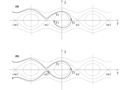
Figure 2: Capture in the $\gamma=\theta-pM-\phi_{x}$ resonance in the phase space ($\gamma$,$\dot{\gamma}$). In the first situation (a) the planet is captured, while in the second one (b) it manages to cross the resonance without being trapped.

Assuming that the $\gamma_{1}$ values comprised between $-\pi/2$ and $\pi/2$ are distributed uniformly, capture inside the resonance will occur for “energy” variations within

$$\left\{{\cal E}:\Delta h(-\pi/2)<\Delta h(\gamma_{1})<0\right\}$$ (92)

from a total of possibilities:

$$\left\{{\cal E}_{T}:\Delta h(-\pi/2)<\Delta h(\gamma_{1})<\Delta h(\pi/2)\right\}\ ,$$ (93)

that is,

$$P_{\mathrm{cap}}^{+}={{\displaystyle\int_{\cal E}d\gamma_{1}}\over{\displaystyle\int_{{\cal E}_{T}}d\gamma_{1}}}=\frac{\Delta h(-\frac{\pi}{2})}{\Delta h(-\frac{\pi}{2})-\Delta h(\frac{\pi}{2})}\ .$$ (94)

Usually tidal torques are very weak, i.e., $\arrowvert\overline{D}(\dot{\gamma})\arrowvert\ll\arrowvert\beta_{m}\arrowvert$, which gives $\gamma_{3}\simeq-\pi/2$, $\gamma_{2}\simeq\pi/2$ and $h\simeq\beta_{m}$. From expression (75) we then write

$$\dot{\gamma}=\mathrm{sign}(\dot{\gamma})\sqrt{2\beta_{m}}\cos\gamma\ .$$ (95)

Replacing it in expression (94) we compute for the capture probability:

$$P_{\mathrm{cap}}^{+}=1+{{\displaystyle\int_{\frac{\pi}{2}}^{-\frac{\pi}{2}}\overline{D}\left(\dot{\gamma}=-\sqrt{2\beta_{m}}\cos\gamma\right)d\gamma}\over{\displaystyle\int_{-\frac{\pi}{2}}^{\frac{\pi}{2}}\overline{D}\left(\dot{\gamma}=+\sqrt{2\beta_{m}}\cos\gamma\right)d\gamma}}\ .$$ (96)

Following an identical reasoning, we can obtain the expression for the capture probability when the spin is increasing from lower rotation rates:

$$P_{\mathrm{cap}}^{-}=1+{{\displaystyle\int_{\frac{\pi}{2}}^{-\frac{\pi}{2}}\overline{D}\left(\dot{\gamma}=+\sqrt{2\beta_{m}}\cos\gamma\right)d\gamma}\over{\displaystyle\int_{-\frac{\pi}{2}}^{\frac{\pi}{2}}\overline{D}\left(\dot{\gamma}=-\sqrt{2\beta_{m}}\cos\gamma\right)d\gamma}}\ .$$ (97)

Let us notice that for even torques in $\dot{\gamma}$, the capture never occurs, while for odd torques it is unavoidable. The capture probability must lie between 0 and 1, but often the results given by expressions (96) and (97) are outside this interval. In those cases, if $P_{\mathrm{cap}}<0$ then $P_{\mathrm{cap}}=0$, and if $P_{\mathrm{cap}}>1$ then $P_{\mathrm{cap}}=1$. For a general dissipation torque in the form

$$\overline{D}(\dot{\gamma})=-K\left[V+\left(\mu_{1}+\mu_{2}\cos 2\gamma\right)\frac{\dot{\gamma}}{n}\right]\ ,$$ (98)

where $K$, $V$, $\mu_{1}$ and $\mu_{2}$ are constants, we compute from expressions (96) and (97):

$$P_{\mathrm{cap}}^{\pm}=2\left[1\pm{{\displaystyle\pi}\over{\displaystyle 2}}{{\displaystyle n}\over{\displaystyle\Delta\omega}}{{\displaystyle V}\over{\displaystyle\mu}}\right]^{-1}\quad\mathrm{with}\quad\mu=\mu_{1}+\frac{\mu_{2}}{3}\ .$$ (99)

6 Dynamical evolution

In this section we analyze the dynamical equations obtained in previous sections. The main goal is to describe both evolution and final stages for the spin under the effect of dissipative effects.

6.1 Rotation rate evolution

The secular variations of the rotation rate are given by expression (79). For a fast rotating planet, the spin is far from any spin-orbit resonance and we can retain only the secular dissipative terms, because $\overline{P_{\mathrm{k}}}=\overline{P(t)}=0$. In this regime we can use a constant-$Q$ model as good approximation for tidal effects (Eq.43). Since all secular terms involved are negative (with $\omega>0$), they can only decrease the rotation rate for any value of the obliquity and eccentricity. This is valid until the slow rotation regime is attained ($\omega\sim n$), where tidal effects can counterbalance the braking effect from core-mantle friction. Once in this regime, two different behaviors are possible: the rotation rate stabilizes around an equilibrium point given by the solution of $T_{\mathrm{k}}=0$ (section 6.3) or the rotation rate is captured in a spin-orbit resonance (section 5).

6.2 Obliquity evolution

6.2.1 Effect of core-mantle friction

According to expression (58), the secular effect of core-mantle friction on the obliquity is given by:

$${{\displaystyle d\varepsilon}\over{\displaystyle dt}}=-K_{f}\cos^{3}\varepsilon\sin\varepsilon\ .$$ (100)

Since $K_{f}>0$ (Eq.59), for any rotation rate the core-mantle friction always brings the equatorial plane of the planet to the same plane as the orbit. We have that $\dot{\varepsilon}$ vanishes for $\varepsilon=0^{\circ}$ and $\varepsilon=180^{\circ}$ (which correspond to stable equilibrium positions) and for $\varepsilon=90^{\circ}$ (unstable equilibrium). Moreover, since $K_{f}$ is proportional to $\alpha^{2}$ (Eq.59) and $\alpha\propto\omega^{-1}$ (Eq.16), the magnitude of both $\dot{\omega}$ and $\dot{\varepsilon}$ will grow as the planet slows down. Thus, for fast rotating planets the core-mantle friction effect can be neglected, but as the planet arrives in the slow rotating regime ($\omega\sim n$), this effect grows so much that it may control the entire evolution of the obliquity (Correia and Laskar, 2003; Correia et al., 2003). The decrease of the rotation rate and the obliquity variations are intimately coupled. Indeed, combining the secular core-mantle friction contributions from expressions (81) and (100), we have that $\dot{\omega}\cos\varepsilon=\omega\dot{\varepsilon}\sin\varepsilon$ (the spin normal component is conserved). As a consequence, for an initial rotation rate $\omega_{i}$ and obliquity $\varepsilon_{i}\neq 90^{\circ}$:

$$\frac{\omega}{\omega_{i}}=\frac{\cos\varepsilon_{i}}{\cos\varepsilon}\ .$$ (101)

Since the obliquity evolves towards $0^{\circ}$ or $180^{\circ}$, i.e., $\arrowvert\cos\varepsilon\arrowvert\rightarrow 1$, the equilibrium rotation rate is attained for $\omega_{e}=\omega_{i}\,\arrowvert\cos\varepsilon_{i}\arrowvert$.

6.2.2 Effect of tides

For a fast rotating planet, using again a constant-$Q$ model, the tidal effects on the obliquity are given by the second equation in system (43). This equation has a single stable point for $\varepsilon=67.11^{\circ}$ (or $x=0.388953$). Thus, since the core-mantle friction effect can be neglected in the fast rotating regime (Eq.100), whatever is the initial obliquity, it will evolve by tidal effect toward this balance point.

Once the planet arrives in the slow rotation regime ($\omega\sim n$), the constant-$Q$ model is no longer suitable and expression (43) no longer valid. Using the viscous model instead (Eq.38), we find that the obliquity still has only one stable point, obtained as the solution of $d\varepsilon/dt=0$:

$$\left\{\begin{array}[]{l l}\varepsilon=\arccos\left(2nE(e)/\omega\right)&\mathrm{if}\quad\omega>2nE(e)\ ,\cr\vskip 6.0pt plus 2.0pt minus 2.0pt\cr\varepsilon=0&\mathrm{if}\quad 2nE(e)\geq\omega>0\ ,\end{array}\right.$$ (102)

where $E(e)=N(e)/\Omega(e)\geq 1$ (Fig.3). Contrary to the fast rotating regime, here the stable point depends on the eccentricity and on the rotation rate of the planet. The stable value for the obliquity decreases as the rotation slows down, stabilizing for circular orbits at zero degrees for rotation rates of $2n$ or smaller, i.e., twice the orbital mean motion. It results that tides, like core-mantle friction, always finish by bringing the planet’s equator to the orbital plane. However, while core-mantle friction allows retrograde final rotations, tides alone only admit direct rotations.

6.3 Equilibrium positions

True equilibrium positions for the spin result from simultaneous balance points for the rotation rate and obliquity, that is

$$\dot{\omega}=0\quad\mathrm{and}\quad\dot{\varepsilon}=0\ .$$ (103)

In section 6.1 we saw that core-mantle friction and tidal effects both decrease the rotation rate for a fast-rotating planet. It is thus impossible to stabilize the spin before the planet arrives in the slow rotation regime. Once in this regime, core-mantle friction becomes dominant over tidal effects (Correia et al., 2003) and drives the obliquity into $0^{\circ}$ or $180^{\circ}$ (Eq.100). It follows then that we must look for stable values of the rotation rate ($\dot{\omega}=0$) when $x=\pm 1$ in order to find the spin equilibrium positions. For these obliquity values, in absence of the spin-orbit resonant term $P_{\mathrm{k}}$, the contribution of the core-mantle friction to the rotation rate vanishes (Eq.81). The equilibrium rotation rate is then determined solely by the tidal effects (Eq.30), that is, when

$$T_{\mathrm{k}}=0\quad\Leftrightarrow\quad\sum_{\sigma}b(\sigma)\Theta^{L}_{\sigma}(\pm 1,e)=0\ ,$$ (104)

or, using the viscous model (Eq.38), simply

$$\omega_{e}=E(e)\,n\ ,$$ (105)

which means that the equilibrium rotation rate increases with the eccentricity of the planet (Goldreich and Peale, 1966; Hut, 1981). This behavior is illustrated in Fig.3.

Figure 3: Evolution of the equilibrium rotation rate $\omega_{e}/n=E(e)$ with the eccentricity when $\varepsilon=0^{\circ}$ using the viscous model. As the eccentricity increases, $\omega_{e}$ also increases. The tidal effects lead the planet to exact resonance when the eccentricity is respectively $e_{1/1}=0$, $e_{3/2}=0.284926803$ and $e_{2/1}=0.392363112$.

6.4 Capture in resonance with $\varepsilon=0^{\circ}$

In section 6.3 we saw that $\varepsilon=0^{\circ}$ or $\varepsilon=180^{\circ}$ correspond to the only two stable positions for the obliquity. For those obliquity values, the non-resonant core-mantle friction contribution to the rotation rate vanishes (Eq.81) and the rotation rate equation (78) can be greatly simplified. Indeed, for $\varepsilon=0^{\circ}$ ($x=1$), we can write

$$\ddot{\gamma}=-{{\displaystyle\beta}\over{\displaystyle c_{m}}}H(p,e)\sin 2\gamma+\overline{D}_{0}(\dot{\gamma})-c_{c}\kappa_{m}P(t)\ ,$$ (106)

where $\gamma=\theta-pM-\phi$ and

$$\overline{D}_{0}(\dot{\gamma})=-K\,\Omega(e)\left[p-E(e)+\frac{\dot{\gamma}}{n}\right]\ .$$ (107)

A similar expression is obtained for the case $\varepsilon=180^{\circ}$ ($x=-1$), we just have to replace $\omega$ by $-\omega$ (see section 3.1). For a circular orbit $(e=0)$, we have $H(p\neq 1,0)=0$ (Tab.1) and thus, the only spin-orbit resonance where capture can occur is the synchronous resonance $(p=1)$. Capture in this resonance always occurs, because according to expression (105) we have $\omega_{e}=n$, since $E(0)=1$.

When the orbital eccentricity increases, according to expression (105) the equilibrium rotation rate $\omega_{e}$ increases to a larger value than $n$ (Fig.3). Since the synchronous resonance width (Eq. 77) for $\varepsilon=0^{\circ}$ is

$$\Delta\omega\simeq n\sqrt{\frac{3(B-A)}{C_{m}}}\ ,$$ (108)

when $\omega_{e}>n+\Delta\omega$, capture in this resonance becomes impossible. The final rotation rate will then be given by $\omega_{e}$ unless capture in a resonance with $p>1$ occurred.

6.4.1 Absence of core-mantle friction

In order to simplify, we will first compute the capture probabilities when there is no contribution from the resonant core-mantle friction, i.e., we neglect the term $c_{c}\kappa_{m}P(t)$ in expression (106). Thus, replacing the expression of the tidal torque (Eq.107) in expression (99), we get for the capture probabilities in the $p$ resonance:

$$P_{\mathrm{cap}}^{\pm}\simeq 2\left[1-\frac{\varrho}{\mu}\pm\frac{1}{\mu}\left(\frac{p-E(e)}{2\Delta\omega/n\pi}\right)\right]^{-1}\ ,$$ (109)

with $\varrho=0$ and $\mu=1$. This expression was first obtained by Goldreich and Peale (1966). It is straightforward that if $(B-A)/C_{m}$ increases (or decreases), the capture in resonance also increases (or decreases). Using the present value for Mercury’s inertia moment $(B-A)/C_{m}\simeq 1.2\times 10^{-4}$ (Anderson et al., 1987) and $e=0.206$, we compute for the 3/2 spin-orbit resonance $P_{\mathrm{cap}}^{+}=7.73$% and $P_{\mathrm{cap}}^{-}=0$. In figure 4 we plotted several examples of capture in different resonances as a function of the eccentricity when the planet is de-spinning from faster rotation rates $(P_{\mathrm{cap}}^{+})$ and when its spin is increasing from slower values $(P_{\mathrm{cap}}^{-})$.

Figure 4: Probability of capture in some spin-orbit resonances for eccentric orbits with $\varepsilon=0^{\circ}$ and $(B-A)/C_{m}=1.2\times 10^{-4}$, when using the viscous model for tides and no core-mantle friction. The dashed line corresponds to a planet increasing its spin from slower rotation rates, while the solid line corresponds to a planet de-spinning from faster rotation rates. In this last situation, for all resonances but the 1/2, as the eccentricity increases, capture probability in higher-order resonances increases. However, it suddenly decays to zero when the equilibrium rotation rate falls outside the resonance width. For the 1/2 resonance, the planet can only be captured when increasing its spin from lower values and with low probability (the maximum being about 1.04% for $e=0.165$).

The most remarkable feature is that the probability grows very fast as the eccentricity increases (or decreases for $P_{\mathrm{cap}}^{-}$), but it suddenly decays to zero. This important behavior was also described by Goldreich and Peale (1966) and it corresponds to a zone where the equilibrium rotation rate does not reach the resonance circulation zone, that is, when

$$\arrowvert\omega_{e}-pn\arrowvert>\Delta\omega\simeq n\sqrt{3H(p,e)\frac{B-A}{C_{m}}}\ .$$ (110)

Thus, the resonance width, which depends mainly on $(B-A)/C_{m}$, not only contributes for the probability of capture, but also determines whenever this capture can occur or not.

6.4.2 Weak coupling

According to expression (86), in the case of a weak coupling ($\kappa^{2}\ll\beta$) we can rewrite expression (106) for $\varepsilon=0^{\circ}$ as

$$\ddot{\gamma}=-{{\displaystyle\beta}\over{\displaystyle c_{m}}}H(p,e)\sin 2\gamma+\overline{D}(\dot{\gamma})\ ,$$ (111)

where

$$\overline{D}(\dot{\gamma}) = \overline{D}_{0}(\dot{\gamma})-c_{c}\kappa_{m}(\dot{\gamma}-\dot{\gamma}_{0})$$ (112)

$$= -K\,\Omega(e)\left[p-E(e)-\varrho\frac{\dot{\gamma}_{0}}{n}+\mu\frac{\dot{\gamma}}{n}\right]\ ,$$ (113)

with

$$\varrho={{\displaystyle c_{c}\kappa_{m}\,n}\over{\displaystyle K\Omega(e)}}\quad\mathrm{and}\quad\mu=1+\varrho\ .$$ (114)

Just before the rotation rate enters the libration zone, its average value is given by $<\dot{\gamma}>=2\Delta\omega/\pi$ (Eq.95). In this regime, $\kappa\ll\sqrt{\beta}\sim\Delta\omega$, and therefore the core is unable to follow the periodic variations in the mantle’s rotation rate. Thus, if the planet is de-spinning from faster rotation rates, we can adopt $\dot{\gamma}_{0}\simeq 2\Delta\omega/\pi$ in expression (113), since capture probabilities are computed when the rotation rate crosses the separatrix between the libration and the circularization zones (Correia and Laskar, 2009). Likewise, if the planet is increasing its spin from slower rotation rates, we use $\dot{\gamma}_{0}\simeq-2\Delta\omega/\pi$ in expression (113).

In this case, the capture probabilities are also given by expression (109), with $\varrho>0$. Since $\mu=1+\varrho>1$, this expression simplifies to $P_{\mathrm{cap}}^{\pm}=2\mu/\left[1\pm\left(\frac{p-E(e)}{2\Delta\omega/n\pi}\right)\right]$, that is, the capture probability is always higher than in absence of the resonant contribution from core-mantle friction. In figure 5, we plotted several examples of capture in different resonances as a function of the eccentricity when the planet is de-spinning from faster rotation rates $(P_{\mathrm{cap}}^{+})$ and when its spin is increasing from slower values $(P_{\mathrm{cap}}^{-})$ using $\nu=10^{-6}\,\mathrm{m}^{2}\mathrm{s}^{-1}$. When comparing with figure 4 (absence of core-mantle friction), we observe that the capture probabilities largely increase, as predicted by Peale and Boss (1977). For instance, with the present eccentricity of Mercury ($e=0.206$) we get $P_{\mathrm{cap}}^{+}=100$% of capture in the 3/2 resonance, which contrasts with $P_{\mathrm{cap}}^{+}=7.73$% in the absence of core-mantle friction. If we used a stronger value of the viscosity, $\nu=10^{-2}\,\mathrm{m}^{2}\mathrm{s}^{-1}$, the capture probability in any of the four resonances plotted in figures 4 and 5 is always one if the eccentricity is higher than $0.002$ and smaller than $0.5$, including for the 1/2 resonance.

Figure 5: Probability of capture in some spin-orbit resonances for eccentric orbits with $\varepsilon=0^{\circ}$ and $(B-A)/C_{m}=1.2\times 10^{-4}$, when using the viscous model for tides and $\nu=10^{-6}\,\mathrm{m}^{2}\mathrm{s}^{-1}$. The dashed line corresponds to a planet increasing its spin from slower rotation rates, while the solid line corresponds to a planet de-spinning from faster rotation rates. When comparing with figure 4 (absence of core-mantle friction), we mainly notice that the eccentricity values that provide 100% of chances of being captured largely increase. For the 1/2 resonance, the planet can only still be captured when increasing its spin from lower values but now also with higher chances (the maximum being about 36% for $e=0.12$).

6.4.3 Strong coupling

Following expression (85), in the case of a strong coupling ($\kappa^{2}\gg\beta$) we can rewrite expression (106) for $\varepsilon=0^{\circ}$ as

$$\ddot{\gamma}=-\beta H(p,e)\sin 2\gamma+\overline{D}(\dot{\gamma})\ ,$$ (115)

where

$$\overline{D}(\dot{\gamma}) = \overline{D}_{0}(\dot{\gamma})-\frac{2\beta}{\kappa}H(p,e)\dot{\gamma}\cos 2\gamma$$ (116)

$$= -K\,\Omega(e)\left[p-E(e)+\left(1+\mu_{2}\cos 2\gamma\right)\frac{\dot{\gamma}}{n}\right]\ ,$$ (117)

and

$$\mu_{2}=\frac{2\beta}{\kappa}\frac{H(p,e)n}{K\Omega(e)}\ .$$ (118)

Thus, according to expression (98), the capture probabilities are still given by expression (109) with $\varrho=0$, $C_{m}=C$, and $\mu=1+\mu_{2}/3$. Since $\mu>1$, the consequences for the capture probability in resonance are the same as in the weak coupling situation (section 6.4.2).

6.5 Capture in resonance with $\varepsilon\neq 0$

The final possible evolutions for the obliquity resulting from dissipative effects are $\varepsilon=0^{\circ}$ or $\varepsilon=180^{\circ}$ (see section 6.3). However, it may happen that when a resonance is crossed, the obliquity is still evolving toward one of the final states. It is then useful to analyze the consequences of a non-zero obliquity. For simplicity, we will first look at the case of a planet without a core. The complete effect with core-mantle friction is discussed in section 6.5.4.

6.5.1 Absence of core-mantle friction

In absence of the core-mantle friction effect, for a non-zero obliquity value, the equilibrium rotation rate $\omega_{e}$ is obtained from expression (38) setting $dL/dt=0$:

$$\omega_{e}={{\displaystyle 2x}\over{\displaystyle 1+x^{2}}}\,E(e)\,n\leq E(e)\,n\ .$$ (119)

Thus, the main consequence of an increasing obliquity is to reduce the equilibrium rotation rate (Fig.6). For zero obliquity, the lowest equilibrium was the synchronous motion ($\omega_{e}=n$), so this configuration was the last possible evolutionary stage for a planet de-spinning from faster spins. Now, if the spin of the planet is not captured in the 1/1 resonance, the planet may evolve to slower final spin configurations, including the 1/2 spin-orbit resonance or below. Indeed, for $\varepsilon>90^{\circ}$ the equilibrium is fixed at a negative rotation rate, allowing the capture in negative resonances as well ($p<0$). Notice, however, that in this case the equilibrium spin always corresponds to prograde rotation, since $\varepsilon>90^{\circ}$.

Figure 6: Evolution of the equilibrium rotation rate $\omega_{e}$ with the obliquity for fixed eccentricities and using the viscous tidal model. The equilibrium rotation rate decreases as the obliquity increases. For $\varepsilon=90^{\circ}$ we have $\omega_{e}=0$ for all eccentricities. Although we have $\omega_{e}<0$ for $\varepsilon>90^{\circ}$, notice that the equilibrium spin still corresponds to a prograde rotation state.

The capture probabilities in all resonances will also vary for different obliquities: not only the tidal torque is different (Eq.38), but also the resonance width will change (Eq.137). From equation (99) we compute:

$$P_{\mathrm{cap}}^{\pm}=2\left[1-\frac{\varrho}{\mu}\pm\frac{1}{\mu}\left(p-{{\displaystyle 2xE(e)}\over{\displaystyle 1+x^{2}}}\right){{\displaystyle n\pi}\over{\displaystyle 2\Delta\omega}}\right]^{-1}\ ,$$ (120)

where $\varrho=0$, $\mu=1$, and $\Delta\omega=\sqrt{2\beta_{m}}=\sqrt{2\beta_{x}/c_{m}}$, with $\beta_{x}$ being given by expression (137). As the obliquity increases, the term in $x$ will decrease and the capture probability will then also decrease. In figure 7 we plot the evolution of the capture probability with the obliquity for the synchronous resonance and two different eccentricities when the planet is de-spinning from faster rotation rates.

Figure 7: Probability of capture in the 1/1 spin-orbit resonance when de-spinning from faster rotation rates for different obliquities and $e=0$ (solid line) or $e=0.2$ (dashed line). We used the viscous tidal model and $(B-A)/C_{m}=1.2\times 10^{-4}$. We see that the capture probability decreases as the obliquity increases. Therefore, unless $\varepsilon<30.66^{\circ}$, the synchronous resonance is no longer the last possible stage for the spin evolution.

For $e=0$ (circular orbit) and low obliquity the capture probability is 100%. As the obliquity increases, this probability decreases fast, and it is close to zero for obliquities higher than $90^{\circ}$. For eccentric orbits, we observe a sort of contrary effect: for some values of the eccentricity, the obliquity can be responsible for an augmentation in the capture probability. Indeed, for high eccentricity and low obliquity the equilibrium rotation rate is always faster than $n$ (Fig.3) and the capture in the synchronous resonance becomes impossible (Fig.4). As the obliquity increases, the equilibrium rotation rate decreases (Eq.119) allowing the planet to approach again the synchronous rotation rate. For $e=0.2$, this occurs when the obliquity is around $60^{\circ}$ (Fig.7).

6.5.2 Capture in the 1/2 resonance

An important consequence of a non-zero obliquity is that the spin can reach previously impossible configurations (section 6.5). Because the capture in the 1/1 synchronous resonance becomes avoidable, the equilibrium rotation rate can evolve to lower values than $n$. In particular, capture in the 1/2 resonance can occur. According to expression (119), for a planet de-spinning from faster rotation rates, unless $\varepsilon>74.5^{\circ}$ the equilibrium rotation rate is above the 1/2 resonance and the capture probability in this resonance is zero (Eq.120). Thus, there is only a chance of capturing the planet if the resonance is crossed with high obliquity (Fig.8).

However, when the initial obliquity of the planet is high, following expression (101) it can happen that the rotation rate becomes inferior to $n/2$ when the obliquity is brought to zero degrees by core-mantle friction. Then, the planet rotation rate will increase towards the equilibrium given by equation (105) and cross the 1/2 resonance from slower rotations. The capture probability is given by $P_{\mathrm{cap}}^{-}$ (Eq.109) with $p=1/2$. Notice also that, as for any resonance different from the 1/1, capture in the 1/2 resonance is only possible for a planet in an orbit with $e>0$ (Tab. 1).

Figure 8: Probability of capture in the 1/2 spin-orbit resonance for eccentric orbits when $\varepsilon=80^{\circ}$, using the viscous tidal model and $(B-A)/C_{m}=1.2\times 10^{-4}$. The solid line corresponds to a planet de-spinning from faster rotation rates, while the dashed line corresponds to a planet increasing its spin from slower rotation rates. According to expression (119), for $\varepsilon>74.5^{\circ}$ the equilibrium rotation rate $\omega_{e}$ is below the 1/2 resonance and for those obliquities $P_{\mathrm{cap}}\neq 0$ (Eq.120).

6.5.3 Capture in “negative” resonances

We now look at “negative” resonances, that is, resonances with $p<0$ (Tab.1). When $\varepsilon<90^{\circ}$, we saw that the equilibrium rotation rate is always positive (Eqs.101 and 119) and negative spin states could not be attained. However, for retrograde planets (whose obliquities are higher than $90^{\circ}$), the equilibrium rotation rate is negative (Eq.119). Since capture in a “positive” resonance can hardly occur for these values of the obliquity (Eq.120), the rotation rate will decrease until the planet starts to rotate in the opposite direction. Once in this situation, the evolution for negative rotation rates can be depicted from the positive rotations case. Due to the symmetry in the spin equations, the couple $(-\omega,\varepsilon)$ behaves identically to the couple $(\omega,\pi-\varepsilon)$. The capture probabilities can then be obtained directly from the positive case: we just have to take into account that the situation corresponding to capture from faster spin rates (slower in modulus) will now correspond to the capture from slower spin rates and vice versa. Contrary to the case with $\varepsilon=0^{\circ}$, the $1/2$ resonance will now be the first resonance to be encountered, followed by the $1/1$.

Capture in “negative” resonances is then a real possibility for planets whose evolution leads the spin to the final obliquity $\varepsilon=180^{\circ}$ (section 6.3). However, notice that, although $p<0$, in this case the resonces always correspond to prograde rotation, since $\varepsilon>90^{\circ}$. These spin-orbit resonances are thus not true negative resonances, and that is why we wrote “negative” with quotes. Indeed, an observer of the planet today is unable to determine if the 3/2 spin-orbit resonance corresponds to the spin state ($\omega/n=3/2$, $\varepsilon=0^{\circ}$) or ($\omega/n=-3/2$, $\varepsilon=180^{\circ}$). A similar result had already been described for the spin of Venus (Correia and Laskar, 2001), but for a different kind of equilibrium.

As a consequence, a true negative resonance will correspond to $p<0$ and $\varepsilon<90^{\circ}$ (or $p>0$ and $\varepsilon>90^{\circ}$). These resonant configurations are not impossible to achieve, but the capture probability is very low (Figs.7 and 9) and we did not register a single case during our numerical simulations.

6.5.4 Core-mantle friction

According to expression (72) the core-mantle friction effect on the spin has two different contributions, one permanent if the obliquity is different from zero (Eq.81) and another arising only near spin-orbit resonances (Eq.68). This last contribution was already present for the case $\varepsilon=0^{\circ}$ and therefore examined in detail in section 6.4.2. As before, its contribution to the capture probabilities for a non-zero obliquity is given by expression (120) with, for weak coupling,

$$\varrho=\frac{2c_{c}\kappa_{m}n}{K(1+x^{2})\Omega(e)}\quad\mathrm{and}\quad\mu=1+\varrho\ ,$$ (121)

or, for strong coupling, $\beta_{m}=\beta_{x}$,

$$\varrho=0\quad\mathrm{and}\quad\mu=1+\frac{4\beta_{x}n}{3\kappa K(1+x^{2})\Omega(e)}\ .$$ (122)

The contribution of the non-resonant core-mantle friction term to the capture probabilities is also easy to compute when we use the linear approximation given by expression (81). In absence of any other dissipative effect, according to expression (99) it is given by

$$P_{\mathrm{cap}}^{+}\simeq-\,4\,{{\displaystyle q}\over{\displaystyle p}}\,{{\displaystyle\sqrt{2\beta_{m}}}\over{\displaystyle n\pi}}<0\ .$$ (123)

This probability is always negative, which means that $P_{\mathrm{cap}}^{+}=0$ for any resonance. Because the spin can only decrease (Eq.101), we also have $P_{\mathrm{cap}}^{-}=0$.

In a more general case, tides are also present and must be taken into account. The total dissipative torque can then be rewritten as

$$\overline{D}(\dot{\gamma})=-K\frac{1+x^{2}}{2}\Omega(e)\left[\left(p-\frac{2xE(e)}{1+x^{2}}+\zeta\right)+\left(1-\zeta\frac{q}{p}\right)\frac{\dot{\gamma}}{n}\right]\ ,$$ (124)

where

$$\zeta=2pn\,{{\displaystyle K_{f}(pn)}\over{\displaystyle K\Omega(e)}}\,{{\displaystyle\left(1-x^{2}\right)x^{2}}\over{\displaystyle 1+x^{2}}}\geq 0$$ (125)

is the ratio between the magnitudes of the core-mantle friction and tidal effects. The total capture probability is now obtained straightforwardly from expression (99) as

$$P_{\mathrm{cap}}^{\pm}=2\left[1-\frac{\varrho}{\mu_{\zeta}}\pm\frac{1}{\mu_{\zeta}}\left(p-{{\displaystyle 2xE(e)}\over{\displaystyle 1+x^{2}}}+\zeta\right){{\displaystyle\pi n}\over{\displaystyle 2\Delta\omega}}\right]^{-1}\ ,$$ (126)

with

$$\mu_{\zeta}=\mu-\zeta{{\displaystyle q}\over{\displaystyle p}}\ ,$$ (127)

$\varrho=0$ and $\mu=1$. If we want to take into account the resonant contribution from core-mantle friction, we just need to modify $\varrho$ and $\mu$ according to expressions (121) and (122). For a dominating core-mantle friction ($\zeta\gg 1$) the previous expression simplifies to expression (123). On the other hand, when $\zeta\rightarrow 0$ (weak core-mantle friction effect) we find expression (120). This is always the case when the obliquity is close to $0^{\circ}$, $90^{\circ}$ or $180^{\circ}$, because $x=0$ or $x=\pm 1$.

Since $\zeta$ is always a positive quantity, expression (126) shows that the capture probability when de-spinning from faster spins is always smaller than it would be without the non-resonant core-mantle friction ($\zeta=0$). In figure 9 we plot the global effect for different spin-orbit resonances and we observe an important reduction in the capture probabilities as the obliquity increases.

Figure 9: Probability of capture in some spin-orbit resonances when de-spinning from faster rotation rates for different obliquities when $e=0.206$ and $(B-A)/C_{m}=1.2\times 10^{-4}$. We compute the probability when tidal effects are considered alone (solid line) and when core-mantle friction is also included, using two different effective viscosities: $\nu=10^{-6}\,\mathrm{m}^{2}\mathrm{s}^{-1}$ (dashed line) and $\nu=10^{-4}\,\mathrm{m}^{2}\mathrm{s}^{-1}$ (dotted line). Although the resonant core-mantle coupling greatly increases the chances of capture in resonance at zero obliquity ($P_{\mathrm{cap}}^{+}=100$% for the 2/1 and 3/2 resonances), for high values of the obliquity this probability considerably decreases, allowing the rotation of the planet to evolve into lower-order equilibrium configurations.

We then conclude that, contrary to the resonant contribution, the non-resonant core-mantle friction effect is responsible for a reduction in the probability of capture for any resonance. Although the resonant core-mantle coupling greatly increases the chances of capture in resonance at zero obliquity ($P_{\mathrm{cap}}^{+}=100$% for the 2/1 and 3/2 resonances), for high values of the obliquity this probability considerably decreases, allowing the rotation of the planet to evolve into lower-order equilibrium configurations such as the 1/1 or the 1/2 resonances.

7 Spin evolution

Using the dynamical equations derived in the former sections we will now simulate the evolution of Mercury’s spin. We start our integrations shortly after the formation of the Solar System and let the planet evolve until present days. This strategy is needed because the present spin configuration of Mercury corresponds to a stable equilibrium and it is impossible to remove it from this state by simply reversing the time.

In order to proceed with our study we need to choose a set of plausible coefficients for the dissipative models described in sections 3 and 4. Although the contribution of these effects to the dynamical equations is well understood, some of the geophysical parameters intervening are poorly known. We will use a set of parameters called the standard model ($k_{2}=0.4$, $Q=50$, $\nu=10^{-6}\,\mathrm{m}^{2}\mathrm{s}^{-1}$), whose choice is described in detail in Correia and Laskar (2009).

7.1 Early evolution

Before looking at the final stages of the spin evolution, where capture in spin-orbit resonances may occur, we will study the behavior of the spin in the early stages after planetary formation. At this epoch Mercury is supposed to rotate much faster than today and any orientation of its axis in space is allowed (Dones and Tremaine, 1993; Kokubo and Ida, 2007). Indeed, the Caloris Basin, a large multi-ringed impact structure is estimated to have been formed by the impact of a 150 km object about 3.85 Gyr ago, at the end of the period known as late heavy bombardment (Murdin, 2000; Strom et al., 2008).

Because Mercury is believed to spin rapidly at the beginning of its evolution ($\omega\gg n$), a constant $Q$ model (section 3.2) seems to be the best choice for tidal evolution. However, for the present slow rotation ($\omega\sim n$), a viscous tidal model is the most appropriate. In our simulations we then interpolate between the two models, adopting $Q=20$ for a fast rotating planet with a constant dissipation model, and $Q=50$ in the limit of slow rotations with a viscous dissipation model. The transition is done at $\omega\sim 10\,n$.

Figure 10: Obliquity evolution with the rotation rate for an initial rotation period of about 32 h ($\omega_{i}=65\,n$). We observe two distinct behaviors: for initial obliquities smaller than $175^{\circ}$ the obliquity is brought to zero. For higher initial obliquities the final obliquity is $180^{\circ}$ and the final rotation rate is negative.

We follow the spin evolution for an initial rotation period of about 32 h ($\omega=65\,n$) and different initial obliquities spanning from $0^{\circ}$ to $180^{\circ}$ (Fig.10). Two distinct behaviors are observed: for initial obliquities smaller than about $175^{\circ}$ the obliquity is brought to zero. For higher initial obliquities the final obliquity is $180^{\circ}$ and the final rotation rate is negative. As discussed in section 6.2, there are only two final possibilities for the obliquity. The bifurcation in these two distinct evolutions is provoked by core-mantle friction. In the fast rotating regime ($\omega\gg n$), this dissipative effect can be neglected (Eq.59) and tidal effects drive the obliquity to the equilibrium value $\varepsilon\simeq 67^{\circ}$ (Eq.43). This is why initial obliquities lower than $67^{\circ}$ increase while higher decrease. Once in the slow rotation regime ($\omega\sim n$), the tidal equilibrium obliquity will move toward zero (Eq.102). However, in this regime, core-mantle friction becomes stronger than tidal effects and drives the final obliquity evolution. When core-mantle friction becomes dominant, if the obliquity is still higher than $90^{\circ}$ it will then end at $180^{\circ}$ (Eq.100). In absence of core-mantle friction the obliquity would always end at zero degrees.

For a stronger core-mantle friction effect, the global picture in figure 10 would not change much, only the critical initial obliquity that triggers the two distinct final evolutions would be lower than $175^{\circ}$. For instance, using $\nu=10^{-4}\,\mathrm{m}^{2}\mathrm{s}^{-1}$ this threshold drops to $170^{\circ}$. It is also important to note that the critical obliquities increase for faster initial rotation rates and decrease for slower ones.

7.2 Final evolution

We now look in detail at the behavior of the spin at the final stages of its evolution. Here the planet will encounter several spin-orbit resonances where the rotation rate may be trapped. Since we are considering the effect of core-mantle friction, we need to take into account its resonant contribution to the rotation rate (Eq.68), as discussed in section 5.2. With the presently known geophysical parameters of Mercury, using the core viscosity $\nu=10^{-2}\,\mathrm{m}^{2}\mathrm{s}^{-1}$, we compute $\kappa^{2}/\beta\sim 10^{-2}\ll 1$, the $\kappa^{2}/\beta$ ratio being smaller for lower viscosity values. Thus, we conclude that we can use the weak coupling approximation (Eq.86) for Mercury, and the evolution of its rotation rate can be described by expression (111). Nevertheless, in our simulations we will integrate simultaneously the mantle (Eq.61) and the core (Eq.64) rotation rates.

As we just saw in previous section, the final evolution of the obliquity is either along $0^{\circ}$ or $180^{\circ}$. We will then first consider the simplified situation where the obliquity already achieved one of the final states ($\varepsilon=0^{\circ}$) when the rotation rate enters the zone of spin-orbit resonances. This will allow us better to compare our results with those from previous studies, for which the obliquity was always held fixed at zero degrees. Because there is no guarantee that at the time of the first resonance crossing the obliquity is already close to zero (Fig.10) and since the capture probabilities also change with the obliquity (section 6.5), we will then look at the evolution of the rotation rate when the obliquity is still varying.

7.2.1 Case $\varepsilon=0^{\circ}$

Once the obliquity reaches $0^{\circ}$ (or $180^{\circ}$), the non-resonant effect of core-mantle friction vanishes (Eqs.81,100). Tidal dissipation will then drive the rotation rate of the planet towards a limit equilibrium value $\omega_{e}$ depending on the eccentricity $e$ and on the mean motion $n$ (Eq.105). In a circular orbit ($e=0$) this equilibrium coincides with synchronization ($\omega_{e}/n=1$), while the equilibrium rotation rate $\omega_{e}/n=1.5$ is achieved for $e_{3/2}=0.284927$ (Fig.3). For the present value of Mercury’s eccentricity ($e=0.206$) we have $\omega_{e}/n=1.25685$. Thus, when Mercury is de-spinning from faster rotation rates it will encounter all spin-orbit resonances with $p\geq 3/2$, and when the spin is increasing from lower values it can be captured in resonances with $p\leq 1/1$. In absence of planetary perturbations, the eccentricity remains constant and each resonance is crossed only once. In order to estimate numerically the probability of capture $P^{+}_{\mathrm{cap}}$, we kept the initial rotation period of 32 h, and ran 2000 simulations for an initial obliquity of $0^{\circ}$ with only slightly different initial libration phase angles. Since the resonant part of the core-mantle friction contribution (Eq.68) modifies the probability of capture (section 6.4), we performed our experiments first in absence of core-mantle friction, and then including this effect with $\nu=10^{-6}\,\mathrm{m}^{2}\mathrm{s}^{-1}$. Results are shown in Table 2.

	no CMF		$\nu=10^{-6}\,\mathrm{m}^{2}/\mathrm{s}$
$\phantom{--}p\phantom{--}$	$\phantom{-}P^{-}_{\mathrm{cap}}\phantom{-}$	- num.–	$\phantom{-}P^{-}_{\mathrm{cap}}\phantom{-}$	- num. –
1/2	1.0	1.0	29.6	31.9
1/1	8.5	7.9	100.0	100.0
$\phantom{--}p\phantom{--}$	$\phantom{-}P^{+}_{\mathrm{cap}}\phantom{-}$	- num.–	$\phantom{-}P^{+}_{\mathrm{cap}}\phantom{-}$	- num. –
3/2	7.7	7.2	100.0	100.0
2/1	1.8	1.7	100.0	100.0
5/2	0.7	1.4	45.8	46.9
3/1	0.3	0.4	22.3	22.3
7/2	0.1	0.1	11.3	11.3
4/1	0.1	-	5.8	5.0
9/2	-	-	3.0	1.5

Table 2: Capture probabilities in several spin-orbit resonances (in percent). The first column ($P^{\pm}_{\mathrm{cap}}$) refers to the theoretical estimation given by expression (109), while the next column (num.) refers to the estimation obtained running a numerical simulation with 2000 different initial conditions. We used $(B-A)/C_{m}=1.2\times 10^{-4}$, and a constant eccentricity $e=0.206$.

In absence of core-mantle friction and using the present eccentricity of Mercury ($e=0.206$), the probability of capture in the 3/2 spin-orbit resonance was numerically estimated to be 7.2%. In their work, Goldreich and Peale (1966) estimated analytically the same probability to be $P_{3/2}=$ 6.7% (Eq.109). With the updated value of the moment of inertia $(B-A)/C_{m}\simeq 1.2\times 10^{-4}$ (Anderson et al., 1987), this probability is increased to 7.7%, which is in a satisfactory agreement with our numerical simulations. The same is also true for all the other resonances (Tab.2).

When we add the effect from core-mantle friction, the numerical simulations are still in a good agreement with the theoretical estimations given by expression (109), showing that they can be used to forecast the behavior of numerical simulations. In this situation the capture probabilities considerably increase for all spin-orbit resonances. In particular, capture probability in the 2/1 resonance also becomes 100%, preventing a subsequent evolution to the 3/2 resonance. This behavior was already expected from our analysis in section 6.4.2, and it is in conformity with the results from Goldreich and Peale (1967) and Peale and Boss (1977), that is, when the effect from core-mantle friction is considered, the probabilities of capture are greatly enhanced.

7.2.2 Case $\varepsilon\neq 0^{\circ}$

The initial obliquity of Mercury is unknown, since a small number of large impacts at the end of the formation process will not average away and may change the obliquity of the planet (Dones and Tremaine, 1993; Kokubo and Ida, 2007). In addition, even for initial low obliquities, during the first stages of the evolution, the strong tidal effects acting on Mercury tend to increase the obliquity (Fig.10). Thus, when the planet arrives in the slow rotation regime ($\omega\sim n$), for which resonance crossing occurs, it is almost certain that the obliquity is higher than zero.

According to expression (119) as the obliquity increases, the equilibrium rotation rate decreases (Fig.6) allowing the spin to evolve into spin-orbit resonances lower than the synchronous rotation ($p=1$). This possibility is also enhanced by the fact that the capture probability in positive resonances ($p>0$) is also reduced for high obliquities (Figs.7 and 9). Thus, when considering a non-zero obliquity we may expect the planet to evolve into resonant configurations with $p<3/2$.

To test these scenarios, we repeated the previous 2000 numerical experiences using several different initial obliquities with $\nu=10^{-6}\,\mathrm{m}^{2}\mathrm{s}^{-1}$. In Table 3 we report the distribution of the different final spins obtained. As expected, we observe a significant modification in the number of captures for all resonances, and for retrograde planets these captures can occur in lower-order resonances than the 3/2.

$\varepsilon_{0}$	–1/2	–1/1	–3/2	–2/1	–5/2	–3/1	–7/2	–4/1	–9/2
$0^{\circ}$	-	-	-	34.3	30.3	18.6	10.6	4.9	1.5
$5^{\circ}$	-	-	-	32.8	31.1	19.1	10.8	4.9	1.5
$10^{\circ}$	-	-	1.0	32.2	28.6	20.3	10.8	5.6	1.5
$15^{\circ}$	-	-	2.5	30.8	29.8	19.8	10.7	5.3	1.3
$30^{\circ}$	-	-	3.9	32.1	29.5	17.9	11.3	4.3	1.0
$45^{\circ}$	-	-	1.7	34.8	27.9	19.1	10.9	5.1	0.8
$60^{\circ}$	-	-	5.0	32.0	28.1	20.0	9.2	5.2	0.8
$75^{\circ}$	-	-	7.4	29.9	28.9	18.6	9.5	4.6	1.3
$90^{\circ}$	-	-	2.4	31.9	29.4	19.2	10.7	5.5	1.0
$105^{\circ}$	-	-	5.3	33.8	27.5	18.7	9.0	4.9	1.0
$120^{\circ}$	-	-	4.2	32.9	29.4	18.5	10.2	3.9	1.1
$135^{\circ}$	-	-	3.3	34.7	28.2	19.0	9.2	5.0	0.8
$150^{\circ}$	-	-	2.5	36.3	29.7	18.1	9.9	3.3	0.4
$165^{\circ}$	-	-	23.6	46.6	23.3	4.6	1.9	-	-
$170^{\circ}$	-	25.5	59.2	11.7	3.2	0.5	-	-	-
$175^{\circ}$	2.4	6.8	6.0	0.8	-	-	-	-	-
$175^{\circ}(*)$	28.2	55.9	-	-	-	-	-	-	-
$180^{\circ}(*)$	31.9	68.1	-	-	-	-	-	-	-

Table 3: Capture probabilities (in percent) in several spin-orbit resonances for different initial obliquities. Tidal effects and full core-mantle friction are included with $\nu=10^{-6}\,\mathrm{m}^{2}\mathrm{s}^{-1}$. We performed a numerical simulation with 2000 close initial conditions with $(B-A)/C_{m}=1.2\times 10^{-4}$ and $e=0.206$. We see that crossing a resonance with an obliquity different from zero substantially modifies the chances of being captured in a specific spin-orbit resonance. $(*)$: these final equilibria are achieved for a final obliquity of $180^{\circ}$ and a negative rotation rate.

For initial obliquities lower than the critical obliquity ($\varepsilon_{0}\approx 175^{\circ}$ for $\nu=10^{-6}\,\mathrm{m}^{2}\mathrm{s}^{-1}$) the capture probability in all resonances is reduced according to expression (126). Indeed, when the resonances are crossed with non-zero obliquity, not only the capture probability resulting from tides is smaller, but there is also a reducing contribution from the core-mantle friction effect (Fig.9). For instance, when the initial obliquity is $\varepsilon_{0}=90^{\circ}$, the 2/1 resonance is crossed with an obliquity around $\varepsilon\simeq 50^{\circ}$, and capture in the 3/2 resonance becomes possible, while it was not for $\varepsilon=0^{\circ}$ (Fig.9). The fraction of captures in this resonance presents some variations between 1% and 7%, because it depends on the probability of not being captured in higher-order resonances (Tab.3).

For initial obliquities higher than $170^{\circ}$ (but still lower than the critical obliquity $175^{\circ}$), we observe that capture in resonances lower than the 3/2 also occurred. The reason is that, as core-mantle friction decreases the obliquity, it also decreases the rotation rate following expression (101). When the obliquity reaches zero, the rotation rate may be lower than the equilibrium rotation rate determined by tides (Eq.105), i.e., $0<\omega<E(e)n$, with $E(0.206)=1.25685$. Then, tides alone will increase the spin toward the equilibrium position, and if $\omega$ is below the spin-orbit resonances 1/2 or 1/1, capture in these resonances can occur. Notice however, that in this case the capture probabilities are given by the expression of $P^{-}_{\mathrm{cap}}$, since the planet crosses the resonance when the spin is increasing from lower rotation rates. This is why capture in the 1/2 resonance is possible (Fig.5).

For initial obliquities higher than the critical value, the obliquity of the planet is always higher than $90^{\circ}$ when the resonances are crossed (Fig.10).Thus, the probability of capture in all “positive” resonances ($p>0$) is very small (Fig.9). In this situation the equilibrium rotation rate given by tides will be set at $\omega=-1.25685\,n$ (Eq.119). A planet with $\omega>0$ will continue to decelerate, skip all the “positive” resonances, reverse its rotation direction, and accelerate its spin rate again. It will then sequentially cross resonances $1/2$ and $1/1$ until it reaches $\omega=-1.25685\,n$, if not captured before in one of those two resonances. The capture probabilities in these two “negative” resonances are the same as for the positive resonances $1/2$ and $1/1$ for a planet with $\varepsilon=0^{\circ}$ when increasing its spin from lower values (section 6.5.3). In the case with $\nu=10^{-6}\,\mathrm{m}^{2}\mathrm{s}^{-1}$, we have a 31.9% chance of capture in the 1/2 resonance and 100% in the 1/1, that is, all the simulations that avoided the 1/2 resonance were then trapped in the 1/1 (Tab.2).

8 Conclusions

In the present work we derived a formalism to describe the complete evolution of the spin of a terrestrial planet like Mercury under the effect of strong solar tides and core-mantle friction. The inclusion of the obliquity in the equations of motion allowed us to compute the capture probabilities in resonance for any initial spin value. Even though zero obliquity is the final equilibrium resulting from dissipative effects, for many sets of initial conditions it is possible that Mercury encounters a resonance with a large obliquity. As we increase the obliquity of the planet, the probability of capture in resonance always decreases, allowing the spin to evolve to unexpected configurations.

The presence of a liquid core and the associated core-mantle friction effect also may lead to a peculiar evolution of the spin. Indeed, if the obliquity is higher than $90^{\circ}$ at the moment this effect becomes dominant over tides, the final obliquity will be set at $180^{\circ}$. In this case the rotation rate evolves into negative values, and the final spin is always prograde.

Another important consequence of core-mantle friction is to produce significant modifications of the capture probabilities in resonance. This effect can be decomposed in two, one resulting from the libration of the mantle near spin-orbit resonances (resonant contribution) and another resulting from different orientations of the core and the mantle spin vectors when the obliquity is not zero (non-resonant contribution). This last effect leads to a decrease in the capture probabilities in resonance, while the first one increases those chances.

Finally, we performed some numerical simulations for Mercury, starting with a fast rotating planet and different obliquity values. This allowed us to study the final distribution possibilities for the rotation rate. Higher-order resonances than the 3/2 were already expected, since Mercury had to cross them when de-spinning from faster rotation rates. However, we could also observe lower-order resonant configurations such as the synchronous or the 1/2 spin-orbit resonance. For retrograde planets, “negative” resonances ($p<0$) were also observed, but also corresponding to prograde final states, since $\varepsilon=180^{\circ}$. The present formalism and results should apply more generally to any extrasolar planet or satellite with a core and whose evolution led to cross spin-orbit resonances.

The synchronous resonance can also be achieved for zero obliquity if the chaotic evolution of the eccentricity is taken into account, when very low values of the eccentricity destabilize higher-order resonances and drive the planet’s rotation towards the 1/1 resonance (Correia and Laskar, 2004, 2009). This cannot occur for the present value of the eccentricity ($e=0.206$). In a forthcoming study we will include the contribution of planetary perturbations, which will require massive numerical simulations. This will add the contribution of the variation of eccentricity, already taken into account by Correia and Laskar (2009), but in addition, using the formalism that has been developed in the present work, we will be able also to take into account the large chaotic variations of the planet’s obliquity resulting from planetary perturbations (Laskar and Robutel, 1993).

Appendix A The mean potential energy

In section 2.2 we eliminate the fast angles $\theta$ and $v$ from the potential energy ${\cal U}$ by expanding the true anomaly $v$ in series of the mean anomaly $M$ and then by taking the average of ${\cal U}$ over $\theta$ and $M$. However, resonant terms with argument $(\theta-pM)$ appear in the expression of the potential energy (Eqs. 7, 9) that must be taken into account to the mean potential energy $\overline{\cal U}$ (Eq. 18). Here we give the derivation of the amplitudes $\beta_{x}$ and $\beta_{r}$ as well as the respective phase angles $\phi_{x}$ and $\phi_{r}$.

Let ${\cal U}_{r}$ be the resonant part of the potential energy (Eq. 7)

$$\frac{8\,{\cal U}_{r}}{C}=-2\,\beta\left(\frac{a}{r}\right)^{3}F(\theta,w,\varepsilon)\;,$$ (128)

where $\beta$ is given by expression (17). We can rewrite ${\cal U}_{r}$ as the real part of

$$\frac{8\,\hat{\cal U}_{r}}{C} = -\beta\left(\frac{a}{r}\right)^{3}\left[2(1-x^{2})\mathrm{e}^{\mathrm{i}2\theta}\phantom{\frac{1}{1}}\right.$$ (130)

$$\left.\phantom{\frac{1}{1}}+(x+1)^{2}\mathrm{e}^{\mathrm{i}(2\theta-2w)}+(x-1)^{2}\mathrm{e}^{\mathrm{i}(2\theta+2w)}\right]\ ,$$

and, averaging over $\theta$ and $w$ using expressions (11) and (12),

$$\frac{8\,\hat{\cal U}_{r}}{C} = -\beta\sum_{p=-\infty}^{\infty}\left\{2(1-x^{2})G(p,e)\mathrm{e}^{\mathrm{i}2(\theta-pM)}\right.$$ (133)

$$\quad+\quad H(p,e)\left[(x+1)^{2}\mathrm{e}^{-\mathrm{i}2\phi}\mathrm{e}^{\mathrm{i}2(\theta-pM)}\right.$$

$$\hskip 62.59596pt\left.\left.+(x-1)^{2}\mathrm{e}^{\mathrm{i}2\phi}\mathrm{e}^{\mathrm{i}2(\theta+pM)}\right]\right\}\ .$$

where $\phi=\varpi+\psi$. Let

$$g=\frac{1}{4}(1-x^{2})G(p,e)\quad\mathrm{and}\quad h^{\pm}=\frac{1}{8}(x\pm 1)^{2}H(\pm p,e)\ .$$ (134)

Retaining only the the resonant terms with argument $(\theta-pM)$ in expression (133), we rewrite expression (128) simply as:

$$\frac{\hat{\cal U}_{r}}{C}=-\underbrace{\beta\left[g+h^{+}\mathrm{e}^{-\mathrm{i}2\phi}+h^{-}\mathrm{e}^{\mathrm{i}2\phi}\right]}_{=\ \beta_{x}\,\mathrm{e}^{-\mathrm{i}2\phi_{x}}}\mathrm{e}^{\mathrm{i}2(\theta-pM)}\ ,$$ (135)

where

$$\left({{\displaystyle\beta_{x}}\over{\displaystyle\beta}}\right)^{2} = \left(g+h^{+}+h^{-}\right)^{2}-4g\left(h^{+}+h^{-}\right)\sin^{2}\phi$$ (137)

$$-4h^{+}h^{-}\sin^{2}2\phi$$

and

$$\tan 2\phi_{x}={{\displaystyle(h^{+}-h^{-})\sin 2\phi}\over{\displaystyle g+(h^{+}+h^{-})\cos 2\phi}}\ .$$ (138)

If $x=1$, we have $\beta_{x}=\beta H(p,e)$ and $\phi_{x}=\phi$. Notice that if $g,h^{\pm}\geq 0$ (which is often the case), we have

$$\beta_{x}\leq\beta\,(g+h^{+}+h^{-})\ ,$$ (139)

and also that the average value over $\phi$ is:

$$\left<\left(\frac{\beta_{x}}{\beta}\right)^{2}\right>_{\phi}=g^{2}+(h^{+})^{2}+(h^{-})^{2}\ .$$ (140)

The amplitude $\alpha_{r}$ and the phase angle $\phi_{r}$ can be similarly obtained from expression (135). Indeed, from expression (20) we have:

$$\frac{d\varepsilon}{dt} = -{{\displaystyle 1}\over{\displaystyle 8\omega\sin\varepsilon}}\left[x\frac{\partial}{\partial\theta}+\frac{\partial}{\partial\psi}\right]\left(\frac{8\,\hat{\cal U}_{r}}{C}\right)$$ (141)

$$= -\underbrace{{{\displaystyle\beta}\over{\displaystyle\omega}}\left[g_{r}+h^{+}_{r}\mathrm{e}^{-\mathrm{i}2\phi}+h^{-}_{r}\mathrm{e}^{\mathrm{i}2\phi}\right]}_{=\ \alpha_{r}\,\mathrm{e}^{-\mathrm{i}2\phi_{r}}}\mathrm{i}\sin\varepsilon\,\mathrm{e}^{\mathrm{i}2(\theta-pM)}\ ,$$ (142)

where

$$g_{r}=-\frac{x}{2}G(p,e)\quad\mathrm{and}\quad h^{\pm}_{r}=\frac{1}{4}(x\pm 1)H(\pm p,e)\ .$$ (143)

The expressions for $\omega\,\alpha_{r}$ and $\phi_{r}$ are respectively given by the expressions for $\beta_{x}$ and $\phi_{x}$ (Eqs. 137, 138), where the quantities $g$ and $h^{\pm}$ are respectively replaced by $g_{r}$ and $h^{\pm}_{r}$.

Appendix B Determination of the expressions for the functions $\Omega(e)$ and $N(e)$

In section 3.2.2 we wrote the spin equations of motion (Eqs. 38) under the effect of tides for a viscous dissipation model. For $\varepsilon=0$, these equations were already obtained by Goldreich and Peale (1966) and Hut (1981). Here we will derive those expressions for any value of the eccentricity and obliquity. We already used them in Levrard et al. (2007), without demonstration. Using the same notation as in sections 2.1 and 3.1, we rewrite the tidal potential (Eq. 27) as:

$${\cal V}^{g}=-k_{2}{{\displaystyle Gm_{\odot}R^{5}}\over{\displaystyle r^{3}r^{\prime 3}}}P_{2}(\cos S)\ ,$$ (144)

with $\cos S=\boldsymbol{\hat{r}}\cdot\boldsymbol{\hat{r}}^{\prime}$, the prime ^′ referring to the interacting body. Assuming that both interacting and perturbing body are in the same orbital plane, we can write

$$\cos S = {{\displaystyle(1+x)^{2}}\over{\displaystyle 4}}\cos(w-w^{\prime}-\theta+\theta^{\prime})$$ (145)

$$+ {{\displaystyle(1-x)^{2}}\over{\displaystyle 4}}\cos(w-w^{\prime}+\theta-\theta^{\prime})$$ (146)

$$+ {{\displaystyle 1-x^{2}}\over{\displaystyle 2}}\left[\cos(w-w^{\prime})\phantom{{{\displaystyle}\over{\displaystyle}}}\right.$$ (148)

$$\hskip 28.45274pt+\left.\cos(w+w^{\prime})\left(\cos(\theta-\theta^{\prime})-1\phantom{{{\displaystyle}\over{\displaystyle}}}\right)\right]\ ,$$

where $w^{\prime}=\varpi^{\prime}+\psi+v^{\prime}$ is the true longitude of date. It is now easy to evaluate the contributions to the spin variations using equations (29). For the variation of the rotation rate we obtain:

$$\frac{dL}{dt}=k_{2}{{\displaystyle 3Gm^{\prime}m_{\odot}R^{5}}\over{\displaystyle r^{3}r^{\prime 3}}}\,\cos S\,{{\displaystyle\partial\cos S}\over{\displaystyle\partial\theta}}\ .$$ (149)

Let $\Delta t$ be the time delay between the perturbation and the planet’s response. Then, assuming $\Delta t$ small and the interacting body the same as the perturbing one ($m^{\prime}=m_{\odot}$), we write (Mignard, 1979, 1980):

$$\theta^{\prime}=\theta(t-\Delta t)\simeq\theta(t)-\frac{d\theta}{dt}\Delta t\simeq\theta-\omega\Delta t$$ (150)

and

$$v^{\prime}=v(t-\Delta t)\simeq v(t)-\frac{dv}{dt}\Delta t=v-n\frac{a^{2}}{r^{2}}\sqrt{1-e^{2}}\Delta t\ .$$ (151)

Substituting the above expressions (150) and (151) into expression (149) for the rotation rate, we have to first order in $\Delta t$:

$$\frac{dL}{dt} \simeq -k_{2}{{\displaystyle 3Gm_{\odot}^{2}R^{5}}\over{\displaystyle r^{6}}}\,\left[\left({{\displaystyle 1+x^{2}}\over{\displaystyle 2}}+{{\displaystyle 1-x^{2}}\over{\displaystyle 2}}\cos(2w)\right)\omega\right.$$ (153)

$$\hskip 71.13188pt-\left.\left(x\,\frac{a^{2}}{r^{2}}\sqrt{1-e^{2}}\right)n\right]\Delta t\ .$$

Using $a/r=(1+e\cos v)/(1-e^{2})$ in the previous expression and averaging it over the mean anomaly $M$ and the longitude of the perihelion $\varpi$, we finally get:

$$\frac{dL}{dt}=-{{\displaystyle Gm_{\odot}^{2}R^{5}}\over{\displaystyle a^{6}}}\,{{\displaystyle 3k_{2}}\over{\displaystyle Q}}\,\left[\left({{\displaystyle 1+x^{2}}\over{\displaystyle 2}}\right)\Omega(e)\,\frac{\omega}{n}-x\,N(e)\right]\ ,$$ (154)

where $Q^{-1}=n\Delta t$,

$$\Omega(e)={{\displaystyle 1+3e^{2}+3e^{4}/8}\over{\displaystyle(1-e^{2})^{9/2}}}$$ (155)

and

$$N(e)={{\displaystyle 1+15e^{2}/2+45e^{4}/8+5e^{6}/16}\over{\displaystyle(1-e^{2})^{6}}}\ .$$ (156)

Appendix C Nomenclature

Symbol	Designation	Eq.
$a$	Mercury’s semi-major axis	11
$A$	minimal moment of inertia	2
$A_{c}$	core’s minimal moment of inertia	44
$b(\sigma)$	tidal dissipation factor	32
$B$	intermediate moment of inertia	2
$c_{c}$	core’s moment of inertia ($c_{c}=C_{c}/C$)	59
$c_{m}$	mantle’s moment of inertia ($c_{m}=C_{m}/C$)	73
$C$	maximal moment of inertia	2
$C_{c}$	core’s maximal moment of inertia	44
$C_{m}$	mantle’s maximal moment of inertia	48
$\overline{D}$	general mean dissipative torque	79
$e$	eccentricity of Mercury’s orbit	11
$E$	total tidal energy	33
$E(e)$	tidal eccentricity function	80
$E_{c}$	core dynamical ellipticity	44
$E_{d}$	dynamical ellipticity	10
$g$	function depending on $x$ and $G(e,p)$	134
$g_{r}$	function depending on $x$ and $G(e,p)$	143
$G$	gravitational constant	2
$G(p,e)$	power series in $e$	11
$h$	constant of motion related to the energy	75
$h^{\pm}$	function depending on $x$ and $H(e,p)$	134
$h_{r}^{\pm}$	function depending on $x$ and $H(e,p)$	143
$H(p,e)$	power series in $e$	12
$\boldsymbol{\mathrm{i}}$	minimal axis of inertia	2
$\boldsymbol{\mathrm{I}}$	reference axis of inertial frame	4
$\tilde{\cal I}_{c}$	core tensor of inertia	44
$\boldsymbol{\mathrm{j}}$	intermediate axis of inertia	2
$\boldsymbol{\mathrm{J}}$	reference axis of inertial frame	4
$\boldsymbol{\mathrm{k}}$	maximal axis of inertia	2
$\boldsymbol{\mathrm{K}}$	normal axis to the ecliptic plane	4
$k_{2}$	second Love number	27
$k_{f}$	fluid Love number	10
$K$	tidal dissipation amplitude	41
$K_{f}$	core-mantle friction amplitude	59
$\boldsymbol{L}$	total angular momentum	49
$\boldsymbol{L}_{c}$	core angular momentum	44
$\boldsymbol{L}_{m}$	mantle angular momentum	48
$m$	Mercury’s mass	2
$m_{\odot}$	solar mass	3
$M$	mean anomaly	11
$n$	mean motion	17
$\boldsymbol{N}$	non-radial inertial pressure torque	44
$N(e)$	tidal eccentricity function	39
$p$	semi-integer indicating the resonance	11
$\boldsymbol{p}$	unit vector for averaged precession	50
$\boldsymbol{P}$	precession torque	47
$P_{\mathrm{cap}}^{\pm}$	probability of capture into resonance	96
$P_{\mathrm{k}}$	projection of $\boldsymbol{P}$ over $\boldsymbol{\mathrm{k}}$	61
$P_{l}$	Legendre polynomials of degree $l$	2
$P_{q}$	projection of $\boldsymbol{P}$ over $\boldsymbol{q}$	56
$P(t)$	function of the precession torque $P_{\mathrm{k}}$	68
$p$	semi-integer for core-mantle friction	82
$\boldsymbol{q}$	unit vector normal to averaged precession	52

Symbol	Designation	Eq.
$Q$	quality factor	33
$\boldsymbol{r}$	radial distance from Mercury’s center	2
$\boldsymbol{r}^{\prime}$	radial distance from Mercury’s center	25
$\boldsymbol{\hat{r}}$	unit vector for $\boldsymbol{r}$	2
$R$	Mercury’s radius	10
$R_{c}$	Mercury’s core radius	46
$s_{g}$	signal function $s_{g}=\mathrm{\omega}$	43
$S$	angle between two directions	25
$\boldsymbol{T}$	tidal torque	47
$T_{\mathrm{k}}$	projection of $\boldsymbol{T}$ over $\boldsymbol{\mathrm{k}}$	61
$T_{q}$	projection of $\boldsymbol{T}$ over $\boldsymbol{q}$	56
${\cal U}$	potential energy	3
${\cal U}_{r}$	resonant part of the potential energy	128
$\overline{\cal U}$	averaged potential energy	15
$v$	true anomaly	4
${\cal V}$	gravitational potential	2
${\cal V}^{\prime}$	scalar potential raising tides	25
${\cal V}^{g}$	tidal potential	27
$w$	true longitude of date	5
$x$	cosine of the obliquity ($x=\cos\varepsilon$)	15
$X$	projection of $\boldsymbol{L}$ on the ecliptic’s normal	19
$\alpha$	precession constant	16
$\alpha_{r}$	libration amplitude	142
$\beta$	libration amplitude	17
$\beta_{m}$	libration amplitude ($\beta_{m}=\beta_{x}/c_{m}$)	73
$\beta_{x}$	libration amplitude	137
$\gamma$	relative rotation angle	74
$\boldsymbol{\Gamma}$	efective friction torque	45
$\boldsymbol{\delta}$	differential core rotation rate	44
$\delta_{\mathrm{k}}$	projection of $\boldsymbol{\delta}$ over $\boldsymbol{\mathrm{k}}$	55
$\delta_{p}$	projection of $\boldsymbol{\delta}$ over $\boldsymbol{p}$	55
$\delta(\sigma)$	tidal phase lag	28
$\delta E_{d}$	residual dynamical ellipticity	10
$\Delta E$	tidal energy dissipated per cycle	33
$\Delta t$	tidal time lag	28
$\Delta\omega$	width of the resonance	76
$\varepsilon$	obliquity	5
$\varepsilon_{i}$	initial obliquity	101
$\zeta$	dimensionless parameter	125
$\theta$	hour angle	5
$\Theta_{\sigma}^{L}$	tidal coefficient	30
$\Theta_{\sigma}^{\varepsilon}$	tidal coefficient	31
$\kappa$	effective coupling parameter	45
$\kappa_{\mathrm{vis}}$	viscous coupling parameter	46
$\kappa^{\prime}$	effective coupling parameter	45
$\kappa_{\mathrm{vis}}^{\prime}$	viscous coupling parameter	46
$\kappa_{m}$	effective coupling parameter ($\kappa_{m}=\kappa/c_{m}$)	65
$\mu$	dimensionless parameter	99
$\mu_{e}$	body rigidity	36
$\mu_{\zeta}$	dimensionless parameter	127
$\nu$	kinematic viscosity	46
$\nu_{e}$	body viscosity	36
$\xi$	internal structure factor	41
$\varpi$	longitude of the perihelion	4

Symbol	Designation	Eq.
$\rho$	Mercury’s mean density	36
$\varrho$	dimensionless parameter	109
$\sigma$	tidal frequency	28
$\tau_{a}$	time constant for damping body tides	35
$\tau_{b}$	time constant for damping body tides	35
$\phi$	libration phase $(\phi=\varpi+\psi)$	15
$\phi_{r}$	libration phase	142
$\phi_{x}$	libration phase	138
$\psi$	general precession angle	19
$\dot{\psi}_{x}$	general precession ($\dot{\psi}_{x}=\dot{\phi}_{x}+\dot{\psi}\cos\varepsilon$)	73
$\boldsymbol{\omega}$	mantle’s rotation rate	48
$\boldsymbol{\omega}_{c}$	core’s rotation rate	44
$\omega_{c}^{\mathrm{k}}$	projection of $\boldsymbol{\omega}_{c}$ over $\boldsymbol{\mathrm{k}}$	63
$\omega_{i}$	initial rotation rate	101
$\omega_{e}$	equilibrium rotation rate	105
$\boldsymbol{\Omega}$	precession angular velocity	48
$\Omega(e)$	tidal eccentricity function	40

References

- Anderson et al. (1987) Anderson, J. D., Colombo, G., Espsitio, P. B., Lau, E. L., Trager, G. B., Sep. 1987. The mass, gravity field, and ephemeris of Mercury. Icarus 71, 337–349.
- Andoyer (1923) Andoyer, H., Mar. 1923. Cours de Mécanique Céleste. Gauthier-Villars, Paris.
- Burns (1976) Burns, J. A., Aug. 1976. Consequences of the tidal slowing of Mercury. Icarus 28, 453–458.
- Colombo (1965) Colombo, G., 1965. Rotational Period of the Planet Mercury. \nat208, 575–578.
- Colombo and Shapiro (1966) Colombo, G., Shapiro, I. I., Jul. 1966. The Rotation of the Planet Mercury. \apj145, 296–307.
- Correia (2006) Correia, A. C. M., Dec. 2006. The core-mantle friction effect on the secular spin evolution of terrestrial planets. \epsl252, 398–412.
- Correia and Laskar (2001) Correia, A. C. M., Laskar, J., Jun. 2001. The four final rotation states of Venus. \nat411, 767–770.
- Correia and Laskar (2003) Correia, A. C. M., Laskar, J., May 2003. Long-term evolution of the spin of Venus II. Numerical simulations. Icarus 163, 24–45.
- Correia and Laskar (2004) Correia, A. C. M., Laskar, J., Jun. 2004. Mercury’s capture into the 3/2 spin-orbit resonance as a result of its chaotic dynamics. \nat429, 848–850.
- Correia and Laskar (2009) Correia, A. C. M., Laskar, J., May 2009. Mercury’s capture into the 3/2 spin-orbit resonance including the effect of core-mantle friction. Icarus 201, 1–11.
- Correia et al. (2003) Correia, A. C. M., Laskar, J., Néron de Surgy, O., May 2003. Long-term evolution of the spin of Venus I. Theory. Icarus 163, 1–23.
- Counselman and Shapiro (1970) Counselman, C. C., Shapiro, I. I., 1970. Spin-Orbit resonance of Mercury. Symposia Mathematica 3, 121–169.
- Darwin (1880) Darwin, G. H., 1880. On the secular change in the elements of a satellite revolving around a tidally distorted planet. Philos. Trans. R. Soc. London 171, 713–891.
- Darwin (1908) Darwin, G. H., 1908. Scientific Papers. Cambridge University Press.
- Defrancesco (1988) Defrancesco, S., Apr. 1988. Schiaparelli’s determination of the rotation period of Mercury: a re-examination. Journal of the British Astronomical Association 98, 146–150.
- Deleplace and Cardin (2006) Deleplace, B., Cardin, P., Nov. 2006. Viscomagnetic torque at the core mantle boundary. \gji167, 557–566.
- Dones and Tremaine (1993) Dones, L., Tremaine, S., May 1993. On the origin of planetary spins. Icarus 103, 67–92.
- Gans (1972) Gans, R. F., 1972. Viscosity of the Earth’s core. \jgr77, 360–366.
- Goldreich (1966) Goldreich, P., Feb. 1966. Final spin states of planets and satellites. \aj71, 1–7.