Binary Quasars at High Redshift II: Sub-Mpc Clustering at $z\sim 3-4$

Abstract

We present measurements of the small-scale ($0.1\lesssim r\lesssim 1\ h^{-1}$Mpc) quasar two-point correlation function at $z>2.9$, for a flux-limited ($i<21$) sample of 15 binary quasars compiled by Hennawi et al. (2009). The amplitude of the small-scale clustering increases from $z\sim 3$ to $z\sim 4$. The small-scale clustering amplitude is comparable to or lower than power-law extrapolations (with slope $\gamma=2$) from the large-scale correlation function of the $i<20.2$ quasar sample from the Sloan Digital Sky Survey. Using simple prescriptions relating quasars to dark matter halos, we model the observed small-scale clustering with halo occupation models. Reproducing the large-scale clustering amplitude requires that the active fraction of the black holes in the central galaxies of halos is near unity, but the level of small-scale clustering favors an active fraction of black holes in satellite galaxies $0.1\lesssim f_{s}\lesssim 0.5$ at $z\gtrsim 3$.

1. INTRODUCTION

With the rapid progress in observational and computational cosmology in the past two decades due to dedicated surveys and numerical simulations, it is now possible to study the quasar population within the hierarchical structure formation framework (e.g., Kauffmann & Haehnelt 2000; Volonteri, Haardt & Madau 2003; Wyithe & Loeb 2003; Hopkins et al. 2008; Shankar et al. 2008, 2009; Shen 2009). If luminous quasars are the progenitors of the most massive galaxies today, then they occupy the rare peaks in the initial density fluctuation field, i.e., they are biased tracers of the underlying matter distribution (e.g., Bardeen et al. 1986; Efstathiou & Rees 1988; Cole & Kaiser 1989; Djorgovski 1999; Djorgovski et al. 1999). The quasar two-point correlation function has now been measured for large survey samples to unprecedented precision (e.g., Porciani et al. 2004; Croom et al. 2005; Myers et al. 2006, 2007a; Shen et al. 2007, 2008, 2009; da Ângela et al. 2008; Ross et al. 2009). These studies suggest that quasars live in massive dark matter halos of $M_{\rm halo}\gtrsim\ {\rm a\ few}\times 10^{12}\,h^{-1}M_{\odot}$; their bias relative to the underlying matter increases rapidly with redshift. However, such studies are unable to probe the smallest scales ($r\lesssim 1\,h^{-1}$Mpc), where matter evolves nonlinearly and the distributions of quasars within dark matter halos start to play a role in determining their clustering properties. This is because fiber-fed multi-object spectroscopic surveys usually cannot observe two targets closer than the fiber collision scale $\sim 1^{\prime}$.

Hennawi et al. (2006) compiled a sample of close quasar binaries at $z<3$ by spectroscopic follow-up observations of candidates selected from the Sloan Digital Sky Survey (SDSS; York et al. 2000) imaging data. Using this binary sample, they measured the correlation function down to scales as small as $R_{\rm prop}\sim 15\,$kpc, where $R_{\rm prop}$ is the transverse separation in proper units; they confirmed and extended previous tentative claims (e.g., Djorgovski 1991) that quasars exhibit excess clustering on small scales (most notably at $R_{\rm prop}\lesssim 40\,{\rm kpc}$) compared with the naive power-law extrapolation of the large-scale correlation function. This small-scale excess clustering was confirmed by Myers et al. (2007b, 2008) in a more homogeneous sample, albeit at a lower level of “excess”.

The large-scale quasar correlation function has now been measured at high redshift ($z\gtrsim 3$, Shen et al. 2007), where quasars cluster much more strongly than their low redshift counterparts. It is natural to extend the work of Hennawi et al. (2006) to study the small-scale quasar clustering at $z>3$. However, such investigations are challenging for two reasons: first, the number density of the quasar population drops rapidly after the peak of quasar activity at $z\sim 2-3$ (e.g., Richards et al. 2006); second, quasar pairs on tens of kpc to $1\,$Mpc scales are rare occurrences – only $\lesssim 0.1\%$ of quasars have a close quasar companion with comparable luminosity. Hence a large search volume is needed to build up the statistics. Hennawi et al. (2009, hereafter Paper I) have, for the first time, compiled such a binary quasar sample at $z\gtrsim 3$, which we use here to study the clustering of quasars on small-scales.

The rareness of close quasar pairs is not in direct contradiction with the major merger scenario of quasar triggering, because the probability that two quasars are triggered and identified simultaneously during the early stage of a major merger (i.e., with separations on halo scales rather than on galactic scales) is low in theoretical models (e.g., Volonteri et et al. 2003; Hopkins et al. 2008). However, even a handful of close quasar pairs will contribute significantly to the small-scale clustering amplitude because the mean number density of quasars is so low that the expected number of random companions on such small scales is tiny. Also note that although quasar pairs with comparable luminosities are rare, there might be more fainter companions (i.e., low luminosity AGN or fainter quasars) around luminous quasars (e.g., Djorgovski et al. 2007), as expected from the hierarchical merger scenario.

In this paper we measure the small-scale quasar clustering at $z\gtrsim 3$ using a set of 15 quasar pairs in the sample of Paper I. We adopt the same cosmology as in Paper I, with $\Omega_{m}=0.26$, $\Omega_{\Lambda}=0.74$ and $h=0.7$. Comoving units will be used unless otherwise specified, and we use subscript _prop for proper units.

2. The Sample

Our parent sample is the high-redshift binary quasar catalog presented in Paper I. This sample includes 27 quasar pairs with relative velocity $|\Delta v|<2000\,{\rm km\,s^{-1}}$ at $2.9<z<4.5$, down to a limiting magnitude $i<21$ after correcting for Galactic extinction, selected over $8142$ ${\rm deg}^{2}$ of the SDSS imaging footprint prior to DR6 (Adelman-McCarthy et al. 2008). The detailed target selection criteria, completeness analysis, and follow-up spectroscopy can be found in Paper I. To construct our clustering subsample, we first exclude eight pairs that failed to pass the selection criteria (for which the completeness cannot been quantified) described in §2 of Paper I, leaving 19 pairs. Second, the follow-up spectroscopic observations are the most complete out to an angular separation $\theta\approx 60^{\prime\prime}$, because those targets were assigned higher priority for follow-up spectroscopy, and therefore we restrict ourselves to pairs with angular separation $\theta<60^{\prime\prime}$; this restriction excludes one pair at $z<3.5$ and three pairs at $z>3.5$. Our final clustering subsample thus includes 15 pairs with seven pairs at $z<3.5$ and eight pairs at $z>3.5$, with projected comoving separations $R\sim 0.1-1\,h^{-1}$Mpc and proper separations $R_{\rm prop}\sim$ a few tens to a few hundreds of kpc (see fig. 8 of Paper I).

The sparseness of the sample requires different techniques for measuring the clustering strength, from the traditional binned $w_{p}$ statistic (e.g., Davis & Peebles 1983). Here we adopt the Maximum-Likelihood (ML) approach used in Shen et al. (2009), as described below. We report our ML estimates and statistical uncertainties of the small-scale clustering in §2.1; the systematic uncertainties are discussed in §2.2. To reduce the impact of the selection incompleteness at $z\sim 3.5$ due to stellar contaminants (see Paper I), and to explore redshift evolution, we measure the small-scale clustering in two redshift bins: $2.9<z<3.5$ (low-$z$) and $3.5<z<4.5$ (high-$z$).

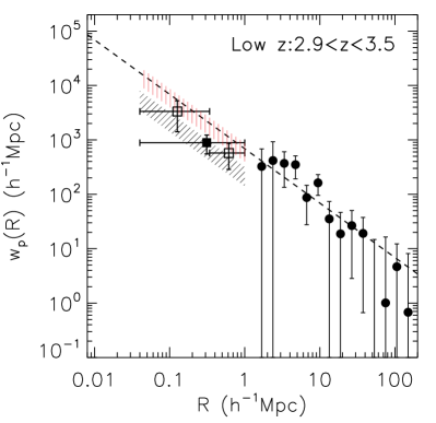
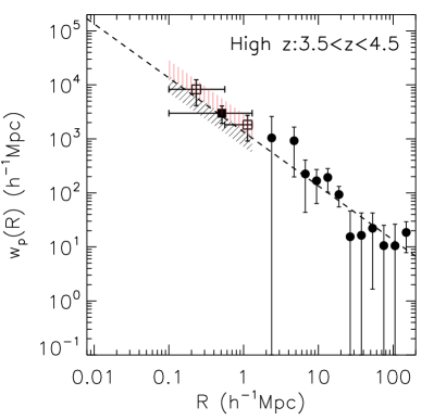
Figure 1.— Measurements of the small-scale clustering for the low-$z$ bin (left) and high-$z$ bin (right). Filled circles are the large-scale correlation function data from Shen et al. (2007, the all sample) and dashed lines are their power-law fits with fixed slope $\gamma=2$. Squares are our estimate of $w_{p}$ using Eqn. (4), estimated in a large radial bin (filled) and two smaller radial bins (open). Points are placed at the logarithmic mean of pair separations in the bin, horizontal error bars show the bin size, and vertical error bars show Poisson errors. The black hatched regions show our ML power-law fits to the small-scale pairs (§2.1; $f_{\rm spec}=1$), with the vertical extent enclosing the 1$\sigma$ statistical uncertainty from the ML fitting. If we assume minimal spectroscopic completeness, $f_{\rm spec}=0.38$ (0.52) for the low-$z$ (high-$z$) bin, the ML results are shown as red hatched regions (see §2.2). These estimates, however, should be considered as solid upper limits.

2.1. Clustering Measurements

Here we recast the ML approach of Shen et al. (2009). We choose a power-law model for the underlying correlation function: $\xi(r)\equiv(r/r_{\rm 0,ML})^{-\gamma_{\rm ML}}$. We then compute the expected number of quasar pairs within a comoving cylindrical volume with projected radius $R$ to $R+dR$ and half-height $\Delta H=20\ h^{-1}$Mpc. This half-height is chosen to reflect our velocity constraint in defining a quasar pair and to minimize the effects of redshift distortions and errors. Assuming Poisson statistics, the likelihood function can be written as:

$${\cal L}=\prod_{i}^{N}e^{-\mu_{i}}\mu_{i}\prod_{j\neq i}e^{-\mu_{j}}\ ,$$ (1)

where $\mu=2\pi Rh(R)\,dR$ is the expected number of pairs in the interval $dR$, the index $i$ runs over all pairs in the sample and the index $j$ runs over all the elements $dR$ in which there are no pairs. The expected pair surface density $h(R)$ is given by

$$h(R)=\displaystyle\frac{1}{2}\int_{z_{\rm min}}^{z_{\rm max}}f_{\rm comp}(z)n^{2}(z)\,dV_{c}\int_{-\Delta H}^{\Delta H}[1+\xi(\sqrt{R^{2}+H^{2}})]dH\ ,$$ (2)

where $n(z)$ is the cumulative quasar luminosity function down to a limiting magnitude (in this case $i=21$), $f_{\rm comp}(z)$ is the completeness in selecting binary candidates for follow-up spectroscopy as quantified in Paper I (see their fig. 7), and $V_{c}$ is the comoving volume between redshifts $z_{\rm min}$ and $z_{\rm max}$ covered by the binary survey. The factor of $1/2$ in eqn. (2) removes duplicate counts of pairs.

Note we only consider the completeness in target selection $f_{\rm comp}\equiv f_{\rm targ}$ (i.e., the fraction of quasar binaries that would have been selected by the algorithm in Paper I) throughout this section. We discuss the effects of the completeness of the spectroscopic follow-up of survey candidates (i.e., the fraction of targets that have been observed), $f_{\rm spec}$, in §2.2.

Defining the usual quantity $S\equiv-2\ln{\cal L}$ we have

$$S\equiv-2\ln{\cal L}=2\int_{R_{\rm min}}^{R_{\rm max}}2\pi Rh(R)\,dR-2\sum_{i}^{N}\ln[h(R_{i})]\ ,$$ (3)

with all the model-independent additive terms removed. Here $[R_{\rm min},R_{\rm max}]$ is the range of comoving scales over which we search for quasar pairs. To include all observed pairs with angular separation $\theta<60^{\prime\prime}$, we choose $[R_{\rm min},R_{\rm max}]=[0.04,1]\ h^{-1}$Mpc for the low-$z$ bin and $[R_{\rm min},R_{\rm max}]=[0.1,1.3]\ h^{-1}$Mpc for the high-$z$ bin. We verified that our results were not sensitive to the exact values of these limits. If we fit both $r_{\rm 0,ML}$ and $\gamma_{\rm ML}$ we found that the best-fit model favors $\gamma_{\rm ML}>2.3$ for both redshift bins, a value substantially steeper than the slope on large scales, $\gamma\sim 2$ (e.g., Shen et al. 2007). However, the spectroscopic completeness, $f_{\rm spec}$, probably depends on angular separation, because we tended to observe the closest candidates first; this may introduce an artificially steep slope in the correlation function. Therefore we fix the slope $\gamma_{\rm ML}=2$ (i.e., close to the measured slope of the large-scale correlation function, Shen et al. 2007) and minimize the merit function $S$ with respect to $r_{\rm 0,ML}$ only. A power-law slope $\gamma\sim 2$ is also found for the clustering of SDSS LRGs to $z\sim 0.4$ (e.g., Masjedi et al. 2006) and photometric SDSS quasars (e.g., Myers et al. 2006, 2007a) over a wide range of scales down to $r=0.01\,h^{-1}$Mpc .

Alternatively, we may estimate the projected correlation function, i.e., the $w_{p}$ statistic, for these pairs. Following the definition of $w_{p}$ (e.g., Davis & Peebles 1983), we have

$$w_{p}(R) = \displaystyle 2\int_{0}^{\infty}dH\xi_{2D}(R,H)=\displaystyle 2\int_{0}^{\infty}\bigg{(}\frac{DD}{RR}-1\bigg{)}dH$$ (4)

$$\approx \displaystyle 2dH\frac{\sum DD}{RR}\approx\displaystyle\frac{4N_{\rm pair}}{(\int_{z_{\rm min}}^{z_{\rm max}}f_{\rm comp}n^{2}dV_{c})\pi(R_{2}^{2}-R_{1}^{2})}\ ,$$

where $\pi(R_{2}^{2}-R_{1}^{2})$ is the projected comoving area of the cylindrical annulus over which we search for pairs, $R$ is the geometric mean pair separation in the bin, $n(z)$ is the cumulative quasar number density, $N_{\rm pair}\equiv\Sigma DD$ is the observed number of quasar pairs in the bin, and $RR$ is the expected number of random-random pairs in the cylindrical shell with radii $(R_{1},R_{2})$ and height $dH$. Note that there are some approximations and ambiguities involved in Eqn. (4), such as the position of the bin center, hence it can only be treated as a crude estimate for $w_{p}$.

For both the ML approach and the $w_{p}$ statistic we need to estimate the integral $\int_{z_{\rm min}}^{z_{\rm max}}f_{\rm comp}n^{2}dV_{c}$. This requires knowledge of the faint end of the luminosity function ($i<21$) of quasars at redshift $2.9<z<4.5$. We have searched the literature for usable LF within these redshift and luminosity ranges (e.g., Wolf et al. 2003; Jiang et al. 2006; Richards et al. 2006; Hopkins et al. 2007). The Jiang et al. (2006) LF data probe sufficiently faint but do not extend to $z>3.6$; the Richards et al. (2006) data have the desired redshift coverage but do not probe deep enough. By comparing the Richards et al. LF with the COMBO-17 LF (Wolf et al. 2003), we found that the COMBO-17 PDE fit gives better estimates of the LF at $z>3.5$, e.g., it agrees well with the Richards et al. LF at the high luminosity end, and produces the expected flattening at fainter luminosities. Motivated by these comparisons, we adopt a combination of the Jiang et al. fit (at $z<3.5$) and the COMBO-17 PDE fit (at $z>3.5$) for the model LF, scaled to our standard cosmology. We estimate an uncertainty in the cumulative number density ($i<21$) of $\sim 20\%$, based on the statistical uncertainties in these LF fits and comparison between these optical LFs and the bolometric LF compiled by Hopkins et al. (2007), where the faint end LF at these redshifts is further constrained by X-ray data. This estimate of uncertainty in the model LF is, however, conservative at $z>3.5$, since there are no direct optical LF measurements down to $i=21$ within this redshift range. We will discuss the contribution of the uncertainty in the LF to the systematic errors in our small-scale clustering measurements, in §2.2.

Our clustering measurements are summarized in Fig. 1, where we plot for comparison the large-scale ($R\gtrsim 2\ h^{-1}$Mpc) correlation function data from Shen et al. (2007, the all sample), for the low-$z$ (left) and high-$z$ (right) bins respectively. The ML approach yields $r_{\rm 0,ML}=8.31^{+1.77}_{-1.61}\ h^{-1}$Mpc for the low-$z$ bin, and $r_{\rm 0,ML}=18.22^{+3.47}_{-3.12}\ h^{-1}$Mpc for the high-$z$ bin, where errors are $1\sigma$ statistical only; these results are shown as black hatched regions whose horizontal and vertical extent encloses the fitting range and statistical errors. For the binned $w_{p}$ statistic, we take all the pairs and use Eqn. (4) to estimate $w_{p}$ for the two redshift bins with Poisson errors. We then plot the $w_{p}$ estimates at the (geometric) mean values of separations $\langle R\rangle$ as filled squares in Fig. 1. To indicate the uncertainties in the bin center, we draw horizontal error bars which enclose the fitting ranges in the ML approach. In both redshift bins we further divide the pairs into two radial bins (with more or less equal number of pairs each), with the dividing scale $R=0.34$ and $0.56\,h^{-1}$Mpc for the low-$z$ and high-$z$ cases (the dividing scale is set by the geometric mean of the maximum separation of observed pairs in the inner bin and the minimum separation of observed pairs in the outer bin). The $w_{p}$ estimates for the divided $R$ bins are shown in open squares in Fig. 1. The results of the $w_{p}$ statistic are consistent with the ML results within the errors. However, due to the ambiguity of placing bin centers when there are only a few pairs, the $w_{p}$ data points cannot be used in the power-law fit. Our ML approach is not subject to such ambiguities, and therefore provides reliable clustering measurements. We tabulate the ML results in Table 1.

Table 1Estimates of $r_{0}$ for fixed power-law ($\gamma=2$) correlation functions

	$r_{\rm 0,ML}$ ($f_{\rm spec}=1$)	$r_{\rm 0,ML}$ (lowest $f_{\rm spec}$)	$r_{0}$ (large-scale)
	$h^{-1}$Mpc	$h^{-1}$Mpc	$h^{-1}$Mpc
low-$z$	$8.31^{+1.77}_{-1.61}$	$13.81^{+2.82}_{-2.52}$	$14.79\pm 2.12$
high-$z$	$18.22^{+3.47}_{-3.12}$	$25.43^{+4.76}_{-4.28}$	$20.68\pm 2.52$

Note. — The second column lists our ML results assuming spectroscopic completeness $f_{\rm spec}=1$ (§2.1). The third column lists ML upper limits assuming the lowest $f_{\rm spec}$ (§2.2). The fourth column lists the large-scale correlation lengths from Shen et al. (2007, the all sample). Uncertainties are 1$\sigma$ statistical only.

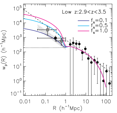
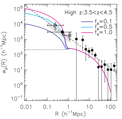
Figure 2.— HOD model predictions for a flux limit of $i<21$ compared with the clustering data (notations are the same as Fig. 1). The solid lines are the HOD predictions, where the dotted lines are the two-halo term contribution to $w_{p}$. Three HOD models with satellite halo duty cycle $f_{s}=0.1$ (blue), $0.5$ (cyan) and $1.0$ (magenta) are presented. For clarity, we have removed the upper limits on the small-scale clustering shown in Fig. 1 (the red hatched regions).

2.2. Systematic Uncertainties

Here we give some quantitative estimation of the systematic uncertainties in our ML results. The two major systematics come from the adopted luminosity function and the sample completeness. Our model luminosity function is quite uncertain down to $i=21$, especially at $z>3.5$ where no direct optical LF data are available. As we described above, the uncertainty in the LF is $\sim 20\%$. In addition, the relative uncertainty in our pair target selection completeness is $\lesssim 10\%$ (Paper I). These taken together, introduce a systematic uncertainty in the best-fit $r_{\rm 0,ML}$ of $\sigma_{r_{\rm 0}}=\pm 1.5\,h^{-1}$Mpc and $\pm 3.1\,h^{-1}$Mpc for the low-$z$ and high-$z$ bins, respectively; these values are comparable to the statistical uncertainties reported above.

In addition, our spectroscopy is incomplete even at $\theta<60^{\prime\prime}$ – only $\sim 38\%$ and $\sim 52\%$ of the high-priority low-$z$ and high-$z$ binary targets have been observed (see Table 3 of Paper I). Therefore we are undoubtedly missing some quasar pairs and our ML results are lower limits. Because targets further away from the stellar locus were assigned higher priority (Paper I), it is difficult to assess the effective spectroscopic completeness (because the most promising candidates were observed first); we expect that the effective spectroscopic completeness is larger than $50\%$. In the extreme case $f_{\rm spec}=0.38$ (low-$z$) and $0.52$ (high-$z$), we repeat our ML analysis in §2.1 with $f_{\rm comp}=f_{\rm targ}\times f_{\rm spec}$ and find $r_{\rm 0,ML}=13.81^{+2.82}_{-2.52}\,h^{-1}$Mpc and $r_{\rm 0,ML}=25.43^{+4.76}_{-4.28}\,h^{-1}$Mpc for the low-$z$ and high-$z$ case respectively, where errors are 1$\sigma$ statistical. These estimates are shown as red hatched regions in Fig. 1 and should be considered as solid upper limits.

The ML results in §2.1 have comparable or lower clustering amplitude at $0.1\lesssim R\lesssim 1\ h^{-1}$Mpc than the extrapolations from the fits for the large-scale correlation functions (Shen et al. 2007, 2009). This does not directly contradict the results in Hennawi et al. (2006) for $z<3$ quasars since: 1) our sample barely probes scales below $R\sim 0.1\,h^{-1}$Mpc where most of the excess clustering occurs for the $z<3$ sample (Hennawi et al. 2006), and 2) the quasar sample in Shen et al. (2007) has $i<20.2$, while our binary sample has $i<21$, thus luminosity-dependent clustering at such high redshift and luminosity ranges might play a role (e.g., Shen 2009). In the next section we show how these small-scale clustering measurements can be used to constrain halo occupation models.

3. Discussion

The small-scale clustering measurements presented above can be used to constrain the statistical occupation of quasars within dark matter halos at $z\gtrsim 3$. Given that we have a poor understanding of the physics of quasar formation, we use a simple phenomenological model relating quasars to halos to model the observed clustering results. The details of the model will be presented elsewhere (Shankar et al., in preparation); below we briefly describe the model assumptions.

We assume there is a monotonic relationship between quasar luminosity and the mass of the host dark matter halo (including subhalos), with a log-normal scatter $\Sigma$ (in dex). Therefore for a flux-limited quasar sample, the minimal halo mass $M_{\rm min}$ and the average duty cycle $f$, defined as the fraction of halos that host a quasar above the luminosity threshold at a given time, can be jointly constrained from abundance matching and the clustering strength (e.g., Martini & Weinberg 2001; Haiman & Hui 2001; Shen et al. 2007; White et al. 2008):

$$n_{{\rm QSO},i<21}(z) = \int_{M_{\rm min}}^{\infty}f(M,z)\Phi_{\rm halo}(M,z)$$ (5)

$$\times {\rm erfc}\bigg{[}\ln\bigg{(}\frac{M_{\rm min}}{M}\bigg{)}\frac{1}{\sqrt{2}\ln(10)\Sigma}\bigg{]}d\log M\ ,$$

where $n_{{\rm QSO},i<21}(z)$ is the cumulative quasar number density with flux limit $i<21$, $M$ is the halo mass, $\Phi_{\rm halo}(M,z)$ is the halo mass function per $\log M$ interval, and $0<f(M,z)<1$ is the average halo duty cycle, which may be a function of both redshift and halo mass.

In general the halo mass function $\Phi_{\rm halo}(M,z)$ includes contributions from both halos ($\Phi_{c}$) and their subhalos ($\Phi_{s}$), where we use the Sheth & Tormen (1999) halo mass function for the former and the unevolved subhalo mass function from Giocoli et al. (2008) for the latter. It is important to use the unevolved mass (i.e., mass defined at accretion before tidal stripping takes place) for subhalos, since subhalos will lose a substantial fraction of mass during the orbital evolution within the parent halo. We denote the average duty cycles for central and satellite halos as $f_{c}$ and $f_{s}$ respectively. Note that we assume halos and subhalos of the same mass host quasars of the same luminosity – of course, subhalos within a given halo will be less massive and thus host quasars fainter on average than the central quasar. The satellite duty cycle $f_{s}$ is the fraction of black holes in subhalos that are active at a given time. The fraction of luminous quasars that are satellites is always small, regardless of $f_{s}$, because the number of massive satellite halos is itself small.

An important consequence of the rareness of binary quasars is that the abundance matching, i.e., Eqn. (5), can be done using central halos only, and we have $f\approx f_{c}$, $\Phi_{\rm halo}\approx\Phi_{c}$ in Eqn. (5); the satellite duty cycle $f_{s}$ will only affect the small-scale clustering strength. In order to simultaneously match the large-scale clustering of $z\gtrsim 3$ quasars (Shen et al. 2007, 2009) and their abundance, Shankar et al. (2008, 2009) found large values of duty cycle $f_{c}\sim 0.5-1$ are needed, as well as small scatter for the quasar-halo correspondence, if the Sheth et al. (2001) bias formula is used (cf. Shen et al. 2007 for the usage of alternative bias formulae). For simplicity we fix $f_{c}=1$ and $\Sigma=0.03$ dex in what follows, which produces adequate fits for the large-scale clustering and abundance matching.

Using Eqn. (5), we determine the minimal halo mass to be $M_{\rm min}\sim 10^{13}\,h^{-1}M_{\odot}$ for both redshift bins. We then use standard halo occupation distribution (HOD) models (e.g., Tinker et al. 2005) to compute the one-halo term correlation function with different values of satellite duty cycle $0<f_{s}<1$.

Fig. 2 shows several examples of our HOD model at $z=3.1$ (left panel) and $z=4$ (right panel) with $f_{s}=0.1$ (blue), $0.5$ (cyan) and $1.0$ (magenta) for a flux limit of $i=21$. Solid lines are the total correlation while the dotted line denotes the two-halo term contribution. As expected, the value of $f_{s}$ has no effect on the large-scale clustering; it only changes the small-scale clustering amplitude. These are not actual fits to the data because the quality of our measurements does not allow a reliable HOD fit. Nevertheless, it seems that some active satellite halos are required, but only $\lesssim 50\%$ of satellite halos can be active at a given time in order not to overshoot the small-scale clustering. This constraint is less stringent if we consider instead the upper limits on the small-scale clustering discussed in §2.2. One potential concern regarding our model is that the adopted subhalo mass function has not yet been tested against simulations for the extreme high-mass end and redshift ranges considered here; nevertheless our model approach demonstrates how the small-scale clustering measurements can be used to constrain quasar occupations within halos. We defer a more detailed investigation on the uncertainties and caveats of our halo models to a future paper (Shankar et al., in preparation).

4. CONCLUSIONS

We have measured the small-scale ($0.1\,h^{-1}{\rm Mpc}\lesssim R\lesssim 1\,h^{-1}{\rm Mpc}$) clustering of quasars at high redshift ($z\gtrsim 3$), based on a sample of $15$ close binaries from Paper I. Strong clustering signals are detected, comparable to or lower than the extrapolations from the large-scale clustering based on SDSS quasar samples. The small-scale clustering increases in strength from $z\sim 3$ to $z\sim 4$, consistent with that of the large-scale clustering (Shen et al. 2007, 2009).

Using a simple prescription relating quasars to dark matter halos, we constrain the average duty cycles of satellite halos at $z\gtrsim 3$ from the small-scale clustering measurements. We found tentative evidence that only $\sim 10\%-50\%$ of satellite halos with mass $\gtrsim 10^{13}\,h^{-1}M_{\odot}$ can host an active quasar (with $i<21$). With the completion of our ongoing binary quasar survey, we will have better estimates of the spectroscopic completeness and therefore will confirm our results.

Future surveys of fainter binary quasars at $z>3$ will increase the sample size and hence the signal-to-noise ratio of the small-scale clustering measurements. These measurements, together with better understandings of the halo/subhalo abundance and clustering at $z>3$ from simulations, will provide important clues to the formation of quasars at high redshift.

References

- (1) Adelman-McCarthy, J. K., et al. 2008, ApJS, 175, 297 (DR6)
- (2) Bardeen, J., Bond, J. R., Kaiser, N., & Szalay, A. S. 1986, ApJ, 304, 15
- (3) Cole, S., & Kaiser, N. 1989, MNRAS, 237, 1127
- (4) Croom, S. M., et al. 2005, MNRAS, 356, 415
- (5) da Ângela, J., et al. 2008, MNRAS, 383, 565
- (6) Davis, M., & Peebles, P. J. E. 1983, ApJ, 267, 465
- (7) Djorgovski, S. 1991, in ASP Conf. Ser. 21, The Space Distribution of Quasars, ed. D. Crampton (San Francisco: ASP), 349
- (8) Djorgovski, S. G. 1999, in ASP Conf. Ser. 193, The Hy-Redshift Universe: Galaxy Formation and Evolution at High Redshift, ed. A. J. Bunker & W. J. M. van Breugel (San Francisco: ASP), 397
- (9) Djorgovski, S. G., Odewahn, S. C., Gal, R. R., Brunner, R. J., & de Carvalho, R. R. 1999, in ASP Conf. Ser. 191, Photometric Redshifts and High-Redshift Galaxies, ed. R. J. Weymann et al. (San Francisco: ASP), 179
- (10) Djorgovski, S. G., Courbin, F., Meylan, G. Sluse, D., Thompson, D., Mahabal, A., & Glikman, E. 2007, ApJ, 662, L1
- (11) Efstathiou, G., & Rees, M. 1988, MNRAS, 230, 5
- (12) Giocoli, C., Tormen, G., & van den Bosch, F. C. 2008, MNRAS, 386, 2135
- (13) Haiman, Z., & Hui, L. 2001, ApJ, 547, 27
- (14) Hennawi, J., et al. 2006, AJ, 131, 1
- (15) Hennawi, J., et al. 2009, submitted (Paper I)
- (16) Hopkins, P. F., Hernquist, L., Cox, T. J., & Kereš, D. 2008, ApJS, 175, 356
- (17) Hopkins, P. F., Richards, G. T., & Hernquist, L. 2007, ApJ, 654, 731
- (18) Jiang, L., et al. 2006, AJ, 131, 2788
- (19) Kauffmann, G., & Haehnelt, M. 2000, MNRAS, 311, 576
- (20) Martini, P., & Weinberg, D. H. 2001, ApJ, 547, 12
- (21) Masjedi, M., et al. 2006, ApJ, 644, 54
- (22) Myers, A. D., et al. 2006, ApJ, 638, 622
- (23) Myers, A. D., et al. 2007a, ApJ, 658, 85
- (24) Myers, A. D., et al. 2007b, ApJ, 658, 99
- (25) Myers, A. D., et al. 2008, ApJ, 678, 635
- (26) Porciani, C., Magliocchetti, M., & Norberg, P. 2004, MNRAS, 355, 1010
- (27) Richards, G. T., et al. 2006, AJ, 131, 2766
- (28) Ross, N. P., et al. 2009, ApJ, 697, 1634
- (29) Shankar, F., Crocce, M., Miralda-Escudé, J., Fosalba, P., & Weinberg, D. H. 2008, arXiv:0810.4919
- (30) Shankar, F., Weinberg, D. H., & Miralda-Escudé, J. 2009, ApJ, 690, 20
- (31) Shen, Y. 2009, ApJ, in press, arXiv:0903.4492
- (32) Shen, Y., et al. 2007, AJ, 133, 2222
- (33) Shen, Y., et al. 2009, ApJ, 697, 1656
- (34) Shen, Y., Strauss, M. A., Hall, P. B., Schneider, D. P., York, D. G., & Bahcall, N. A. 2008, ApJ, 677, 858
- (35) Sheth, R. K., Mo, H. J., & Tormen, G. 2001, MNRAS, 323, 1
- (36) Sheth, R. K., & Tormen, G. 1999, MNRAS, 308, 119
- (37) Tinker, J. L., Weinberg, D. H., Zheng, Z., & Zehavi, I. 2005, ApJ, 631, 41
- (38) Volonteri, M., Haardt, F. & Madau, P. 2003, ApJ, 582, 559
- (39) Wolf, C., Wisotzki, L., Borch, A., Dye, S., Kleinheinrich, M., & Meisenheimer, K. 2003, A&A, 408, 499
- (40) White, M., Martini, P., & Cohn, J. D. 2008, MNRAS, 390, 1179
- (41) Wyithe, J. S. B., & Loeb, A. 2003, ApJ, 595, 614
- (42) York, D. G., et al. 2000, AJ, 120, 1579