M31 Globular Cluster Abundances from High-Resolution, Integrated-Light Spectroscopy

Abstract

We report the first detailed chemical abundances for 5 globular clusters (GCs) in M31 from high-resolution ($R\sim$ 25,000) spectroscopy of their integrated light. These GCs are the first in a larger set of clusters observed as part of an ongoing project to study the formation history of M31 and its globular cluster population. The data presented here were obtained with the HIRES echelle spectrograph on the Keck I telescope, and are analyzed using a new integrated light spectra analysis method that we have developed. In these clusters, we measure abundances for Mg, Al, Si, Ca, Sc, Ti, V, Cr, Mn, Fe, Co, Ni, Y, and Ba, ages $\geq$10 Gyrs, and a range in [Fe/H] of $-0.9$ to $-2.2$. As is typical of Milky Way GCs, we find these M31 GCs to be enhanced in the $\alpha$-elements Ca, Si, and Ti relative to Fe. We also find [Mg/Fe] to be low relative to other [$\alpha$/Fe], and [Al/Fe] to be enhanced in the integrated light abundances. These results imply that abundances of Mg, Al (and likely O, Na) recovered from integrated light do display the inter- and intra-cluster abundance variations seen in individual Milky Way GC stars, and that special care should be taken in the future in interpreting low or high resolution integrated light abundances of globular clusters that are based on Mg-dominated absorption features. Fe-peak and the neutron-capture elements Ba and Y also follow Milky Way abundance trends. We also present high-precision velocity dispersion measurements for all 5 M31 GCs, as well as independent constraints on the reddening toward the clusters from our analysis.

1. Introduction

Stellar atmospheres largely retain the chemical composition of the gas from which they formed, and thus contain a record of the gas chemistry of a galaxy throughout its star formation history. The abundances relative to Fe of some key elements, $\alpha$-elements in particular, can be used to identify the timescales and rates of star formation over the lifetime of a galaxy. $\alpha-$elements (C, O, Ne, Mg, Si, S, Ar, Ca, and Ti) are produced primarily in type II supernovae (SNII) (e.g. Woosley & Weaver, 1995) from massive stars and so build up quickly during active star formation epochs, while Fe-peak elements are produced in all supernovae. [$\alpha$/Fe] abundance patterns are therefore particularly useful and have been central to developing our current picture of the assembly and star formation history of the Milky Way and spiral galaxies in general (see Pritzl et al., 2005, and references therein).

Bright, young stars record the current gas phase abundance in a galaxy; to probe the earliest formation times, one must target older, lower mass, fainter stars. It is only recently that individual red giant branch (RGB) stars in our nearest neighbor galaxies in the Local Group have been within reach of the high resolution spectroscopy needed for detailed chemical abundance analysis. These stars in Local Group dwarf galaxies show a much greater range of abundance ratios at all metallicities compared to stars in the Milky Way halo (Venn et al., 2004; Shetrone et al., 2001, 2003; Geisler et al., 2005; Tolstoy et al., 2009), suggesting that they have had a much more complicated star formation history than the halo’s progenitor(s). Detailed abundances beyond the Milky Way and its nearest remaining neighbors are needed to establish the broader patterns of star formation in galaxies of all masses.

Table 1M31 Clusters

Cluster	RA	Dec	V	E(B$-$V)	$M_{Vtot}$	Rgc	[Fe/H]	[$\alpha$/Fe]	HBR
	(2000)	(2000)				(kpc)
G108-B045	00 41 43.26	41 34 21.8	15.83	0.10	$-$8.95	4.87	$-$0.94$\pm$0.27	0.22 $\pm$ 0.19	0.14
G219-B358	00 43 18.01	39 49 13.5	15.12	0.06	$-$9.53	19.78	$-$1.83$\pm$0.22	0.00 $\pm$ 0.27	0.78
G315-B381	00 46 06.47	41 21 00.2	15.76	0.17$b$	$-$9.24	8.8	$-$1.22$\pm$0.43	$\cdots$	$\cdots$
G322-B386	00 46 26.94	42 01 52.9	15.64	0.13	$-$9.24	14.02	$-$1.21$\pm$0.38	0.25 $\pm$ 0.22	0.41
G351-B405	00 49 39.81	41 35 29.4	15.20	0.08	$-$9.52	18.2	$-$1.80$\pm$0.31	$\cdots$	0.71

References. — a. Rich et al. (2005), b. Fan et al. (2008), c. Reddening corrected and using a distance modulus for M31 of ($m-M$)$=24.47$ (Holland, 1998), d. Perrett et al. (2002) e. Low resolution spectroscopic metallicities of Huchra et al. (1991), f. Low resolution [$\alpha$/Fe] of Puzia et al. (2005), g. Horizontal branch morphology ratios (HBR), defined as the ”Mironov Index” = $B/B+R$, where $B$ and $R$ correspond to the number of horizontal branch stars bluer or redder than $V-I=0.5$ in the observed CMD of Rich et al. (2005) Other data: Barmby et al. (2000)

Unfortunately, at $\sim$780 kpc from the Milky Way (Holland, 1998), even M31 is distant enough that older RGB stars are too faint (V$\sim$23) to obtain the required high signal-to-noise ratio (SNR$\sim 60$) and high spectral resolution ($\lambda/\Delta\lambda\sim 20,000$) to measure detailed abundances in individual stars. Fortunately, globular clusters (GCs) can also be targeted. Unlike single stars, high resolution spectra can be obtained of unresolved GCs out to $\sim$ 4 Mpc with current telescopes. GCs are bright enough ($-10<M_{V}<-6$ mag) and have low enough velocity dispersions ($2-20$ km s^-1) that even weak lines ($\sim$15 mÅ) can be detected in spectra of their integrated light. Detailed abundances have never been obtained from unresolved GCs because techniques have not existed to analyze them. We have developed a new method for analyzing high resolution integrated light (IL) spectra of single age, chemically homogeneous stellar populations to obtain detailed element abundances as described in Bernstein & McWilliam (2002, 2005) and McWilliam & Bernstein (2008), hereafter “MB08.”

Our method has been developed and tested on a “training set” of Milky Way and LMC GCs with well determined properties from studies of individual stars. IL spectra of the training set GCs were obtained by scanning a 32$\times$32 arcsec² region of the cluster cores in the Milky Way clusters, and a $12\times 12$ arcsec² region in the LMC. Note that slit scanning is only necessary for the resolved GCs we target in our training set, not for unresolved, extragalactic GCs. The training set GCs were chosen to cover the range of metallicity, horizontal branch morphology, mass, velocity dispersion, and age available in the Milky Way and LMC systems. Using this training set, we have compared abundances determined with our IL method and abundances from the literature determined for individual RGB stars. Based on the Milky Way training set, we estimate empirically that our [Fe/H] abundances are accurate to within $<$ 0.1 dex, and all other element ratios ([X/Fe]) accurate to within $<$ 0.1 dex (see MB08 and S. Cameron et al. 2009, in preparation). We also derive approximate ages ($>$10 Gyr) for our entire Milky Way training set. Using the larger age range of the LMC clusters, which includes clusters as young as $\sim$10 Myr, we have found that our method can clearly distinguish clusters over a large range in age. Our accuracies at the youngest ages are described in a forthcoming paper (J. Colucci et. al 2009, in preparation).

In addition to the fact that GCs are among the oldest stellar populations in galaxies, there is ample evidence that GCs are a good tool for tracing both the early formation of galaxies themselves and star formation throughout their histories. The fact that the number of GCs in a galaxy scales with the total luminosity of the galaxy (e.g. Harris, 1991) suggests that the GCs trace total star formation. Additionally, young massive clusters are seen forming in regions with high star formation rates, such as mergers of gas rich galaxies (e.g. Schweizer & Seitzer, 1998; Whitmore & Schweizer, 1995), indicating that GCs form in major episodes of star formation, throughout the lifetimes of galaxies. While the old age of GCs alone suggest that they record the earliest star formation episodes in galaxies, there is additionally strong evidence that both blue (metal-poor) and red (metal-rich) sub-populations of GCs in normal galaxies correlate with the host galaxy’s luminosity and overall metallicity(e.g. Brodie & Strader, 2006). This suggests that both sub-populations are a record of the formation history of the galaxy, with blue clusters possibly tracing the earliest star formation in dark matter halos and red clusters tracing the later formation after the gas is more enriched. Finally, GCs are also relatively easy spectroscopic targets to analyze because, to first order, they are simple stellar populations (SSPs), and can be approximated with a single age and single metallicity. For all of these reasons, detailed abundance analysis of GC systems is a powerful tool for understanding the formation of galaxies beyond the Milky Way.

M31 is the closest large galaxy to the Milky Way and an ideal target for galaxy formation studies using GCs. Like the Milky Way, M31 has a large system of GCs, most of which are old ($\geq 10$ Gyrs), and has a bimodal metallicity distribution with peaks at [Fe/H]$\sim-1.4$ and [Fe/H]$\sim-0.5$ and a mean of [Fe/H]$\sim-1.2$ (Barmby et al., 2000; Perrett et al., 2002). Barmby et al. (2007) find that M31 and Milky Way GCs are structurally similar, with similar mass-to-light (M/L) ratios, and fall on a single GC fundamental plane. However, there are notable differences that have been observed between the two galaxies. To begin with, M31’s GC system is more than a factor of 2 larger than the Milky Way’s (Galleti et al., 2004), has massive but diffuse GCs (Huxor et al., 2005; Mackey et al., 2006), and metal-poor and compact GCs at very large projected galactocentric radii (Martin et al., 2006; Mackey et al., 2007). There is evidence for young and/or intermediate age GCs in M31 unlike in the Milky Way (Beasley et al., 2004; Puzia et al., 2005), and a significant population of GCs of all metallicities kinematically associated with the thin disk (Morrison et al., 2004). There is also evidence for some chemical differences in M31 GCs; compared to the Milky Way, M31 GCs show enhanced CN molecular lines (e.g. Burstein et al., 1984), and the first estimates of [$\alpha$/Fe] ratios in M31 GCs have indicated it may on average be $\sim$0.1$-$0.2 dex lower than in the Milky Way (Puzia et al., 2005; Beasley et al., 2005). More detailed studies are required to understand what these similiarities and differences imply for the formation history of M31.

Much of what is known about M31 comes from low resolution spectroscopic methods like the “Lick” system (e.g. Faber et al., 1985), which have been used to target spatially unresolved GCs (e.g. Huchra et al., 1991) to obtain the constraints to date on [Fe/H] and [$\alpha$/Fe] ratios (e.g. Puzia et al., 2005; Beasley et al., 2005). These line index systems were originally developed for studying the integrated light of galaxies, which have velocity dispersions of 100$-$300 km s^-1(Faber & Jackson, 1976). With the low velocity dispersions of GCs, individual spectral lines can be resolved with only slightly greater line blending than one finds in individual RGB stars. The accuracy of the line index systems depends on calibrations that are sensitive to abundance ratios and overall metallicity. These limitations make detailed abundance analysis from individual lines, as in our method, an important next step.

In this paper we present the analysis of 5 GCs in M31 using high resolution spectroscopy of their integrated light. These represent the first set of clusters which we have observed as part of an ongoing project to study the GC population in M31 with the goal of constraining the stellar populations and formation history of M31. From these clusters, we derive detailed stellar abundances of old populations in M31 for the first time. We obtain results for 14 elements: Mg, Al, Si, Ca, Sc, Ti, V, Cr, Mn, Fe, Co, Ni, Y, and Ba. We also present ages, velocity dispersions, and reddening constraints for this sample. In § 2, we describe our observations and data reduction. In § 3 we present analysis of the velocity dispersions and implications for our equivalent width abundance analysis. In § 4 we describe our abundance analysis method and present abundance results in § 5. In § 6 we discuss the M31 GC chemical abundances in the contexts of galaxy formation, low resolution spectra line index abundances, and overall consistency with broadband photometric colors and existing Hubble Space Telescope (HST) CMDs.

Table 2Observation Log and Estimated SNR

Cluster	Exposure (s)	SNR (pixel-1)
		4400 Å	6050 Å	7550 Å
G108-B045	16,200	40	60	80
G219-B358	10,500	40	60	70
G315-B381	14,300	30	50	60
G322-B386	12,600	30	50	60
G351-B405	10,800	40	60	80

2. Observations and Reductions

In selecting GC targets in M31, we have focused initially on clusters which are spectroscopically confirmed, and are estimated from low resolution indexes to have abundances in the range -1.8 $<$ [Fe/H] $<$ -0.5 dex. At the time of selection, this was the range in which we were most confident of the accuracy of our analysis based on our previous work with the Milky Way training set clusters described above (MB08 and S. Cameron et al. 2009). The targets were further selected to be relatively well studied, reasonably isolated and well outside of M31’s disk to reduce confusion and the chance of confusion from interloping sources. We also avoided the brightest, most massive GCs while still targeting GCs bright enough to get sufficient SNR in a few hours of observations, as they will have the highest velocity dispersions and thus broader, less pronounced spectral lines,. With this in mind, we have selected these GCs from the Barmby catalog (Barmby et al., 2000). This initial set of GCs has magnitudes between 15 and 16. Magnitudes and spatial information are listed for all of the GCs in Table 1, along with low resolution abundance estimates from the literature and horizontal branch morphologies from HST imaging when available.

Figure 1.— A single frame taken with the Keck I guide camera is shown here to illustrate the relative size of a GC in M31 (half-light radius $\sim$1 arcsec) relative to the $1.7\times 7$ arcsec² slit. The guider images a reflection of the sky off the polished slit plate, so that the slit itself is clearly visible where no image of the sky is reflected.

Figure 2.— Example M31 GC spectra in Lick Mgb region shown decreasing in [Fe/H] from our analysis (top to bottom). Note that this region is dominated by saturated lines and is shown for illustration as a region familiar in low resolution spectra analyses.

For this work we obtained high resolution IL spectra of the M31 globular clusters using the HIRES spectrograph (Vogt et al., 1994) on the Keck I telescope over the dates 2006 September 10$-$14. We used the D3 decker, which provides a slit size of $1".7\times 7.0"$ and spectral resolution of $R=24,000$. The GCs in this sample have half light radii (r_h) between $\sim$0.6”$-$1.1” (Barmby et al., 2007). We calculate from surface brightness profiles in Barmby et al. (2002, 2007) that $\sim$70$-$90$\%$ of the light fell in the $1".7\times 7.0"$ slit for each cluster. An illustration of the observing setup is shown in Figure 1. The wavelength coverage of the HIRES spectra is approximately 3800$-$8300 Å. Exposure times were between 3$-$4 hours for each GC and are listed in Table 2 along with SNR estimates at three wavelengths, one in each HIRES CCD. Data was reduced with the MAKEE software package available from T. Barlow. In analysis of more recent observing runs, we have compared data analyzed with MAKEE and with the HiRes Redux pipeline produced by J. X. Prochaska, which has many routines and strategies in common with the MIKE Redux pipeline. While HiRes Redux produces lower noise spectra overall, and often traces weak orders more accurately, the MAKEE results are accurate and sufficient for our analysis, particularly since we explicitly avoid regions with sky emission or absorption features entirely. Example spectra for the five M31 GCs are shown in Figure 2, where it can be seen that many individual Fe I, Fe II, Mg I and Ti II lines are easily identified.

Table 3Velocity Dispersion Measurements

Cluster	$\sigma_{obs}$	RMS	$N_{ord}$	Error	$\sigma_{best}$	RMS	$N_{best}$	Error	$\sigma_{lit}$
	(km s-1)				(km s-1)				(km s-1)
G108-B045	10.24	0.44	26	0.09	10.14	0.37	9	0.12	9.82 $\pm$ 0.18
G219-B358	10.99	1.00	13	0.28	10.36	0.84	5	0.38	8.11 $\pm$ 0.36
G315-B381	9.87	0.43	28	0.08	9.65	0.41	10	0.13	$<$ 10
G322-B386	11.42	0.58	19	0.13	11.35	0.37	6	0.15	11.49 $\pm$ 0.24
G351-B405	12.29	1.06	16	0.27	12.01	0.41	7	0.15	8.57 $\pm$ 0.45

References. — (a) Djorgovski et al. (1997), (b) Peterson (1989)

Note. — All measured velocity dispersions are given without application of aperture corrections (see § 3). $\sigma_{obs}$ is the mean measured from all usable orders. $\sigma_{best}$ is the mean measured for higher SNR orders between 4800$-$5800 Å.

3. Velocity Dispersions

One of the strengths of our ILS analysis is the amount of information and the number of constraints available in the high resolution spectra. In addition to checks related to the abundance measurements themselves (see § 4.3), we also have overall photometric colors, magnitudes, and internal kinematics (velocity dispersions). Mass estimates from velocity dispersions can also help to constrain the basic initial mass function, contributing to the overall consistency of our understanding of the stellar population. Measurements of the velocity dispersions also tell us the spectral line resolutions we can expect for our abundance analysis. We compare these results to measurements in the literature when available.

We measure velocity dispersions from the high resolution IL spectra of the M31 GCs following the method described in Tonry & Davis (1979), which is implemented in the IRAF task $fxcor$. The GC spectrum is cross correlated on an order by order basis with a suitable template star. The full width at half-maximum of the cross correlation peaks (FWHM_cp) measured by $fxcor$ is then converted to a line-of-sight velocity dispersion ( $\sigma_{obs}$) using an empirical relation between the two. This relation is established by cross correlating the original template star spectrum with artificially broadened versions of itself that are made by convolving it with Gaussian profiles corresponding to $\sigma_{obs}$ of 2$-$25 km s^-1. RGB stars are suitable template stars for old stellar populations; in this analysis, we use a spectrum of HR 8831 (type G8 III) taken during the 2006 September run as the template.

In Table 2 we report $\sigma_{obs}$ and the associated 1-$\sigma$ errors measured for orders between 4000$-$6800 Å. Only orders with high SNR and weak atmospheric absorption are used in the cross correlation. We also avoid orders that include the saturated Balmer lines. Recently, Strader et al. (2009) have found a weak trend of $\sigma_{obs}$ with wavelength in a fraction of the GCs they observed. We do not find any correlations between $\sigma_{obs}$ and wavelength for G108, G315, or G322. However a small correlation exists for G219 and G351. Like Strader et al. (2009), we find $\sigma_{obs}$ decreasing from blue to red orders by $\sim$1 km s^-1. It is unclear if this is due to a color/metallicity mismatch of the GCs and the template star (these two GCs are the more metal-poor ones in our sample) or other systematic effect (see Strader et al., 2009, for a larger discussion). Because of this issue, in Table 2 we have reported $\sigma_{best}$, which is the dispersion obtained for a subset of the highest SNR orders between 4800$-$5800 Å that do not show correlations with velocity dispersion and also give the smallest RMS errors. The number of orders used in each measurement are recorded in columns 4 and 7 of Table  2.

Four of the GCs observed here have $\sigma_{obs}$ measurements in the literature from previous observations by Djorgovski et al. (1997). The spectra used by Djorgovski et al. (1997) were taken with a slightly narrower slit ($1".15\times 7.0"$), which will lead to a velocity dispersion roughly 0.5 km s^-1  larger, which is comparable to the measurement errors. We find that our measurements for G108 and G322 agree with those in Djorgovski et al. (1997) within the quoted errors, but our observed velocity dispersions for G219 and G351 are $2-4$ km s^-1  larger. It is possible that the difference between our results and those of Djorgovski et al. (1997) are due to a difference in $v$sin$i$ of the template star used in the cross correlation. The template used by Djorgovski et al. (1997) has $v$sin$i$= 7 km s^-1. We measure a mean FWHM of 8 km s^-1  from line widths in our template star. Note that this is a combination of the intrinsic stellar line width (including $v$sin$i$) and the instrumental resolution, which is FWHM = 7.7 km s^-1based on an analysis of arc lines taken through the appropriate slit. This suggests that the rotational velocity of the star is quite small (less than or equal to roughly 1 km s^-1  when added in quadrature). The lower $v$sin$i$ of our template could therefore cause the higher inferred $\sigma_{obs}$ found here. Both our measurements and those of Djorgovski et al. (1997) require an additional correction of approximately $+14\%$ to convert $\sigma_{obs}$ to a projected central $\sigma_{v}$ as described in Djorgovski et al. (1997). This is the geometrical correction appropriate to obtain a systemic line of sight velocity dispersion from a velocity dispersion measured within a radius of $2-3\times r_{h}$.

For completeness, we note that Barmby et al. (2007) have predicted aperture velocity dispersions for these same GCs by modeling surface brightness profiles. They have compared their predictions to observations of velocity dispersions in the literature to derive an empirical correction between the two. We note that our velocity dispersion measurements for G219 and G351 are more consistent with the trend derived by Barmby et al. (2007) than the measurements by Djorgovski et al. (1997). A velocity dispersion of $12.1\pm 1.3$ km s^-1  has also been measured by Strader et al. (2009), which is more consistent with the value we measure.

Finally, we report the first velocity dispersion measurement from high SNR, high spectral resolution, IL spectra for G315-B381. Our measurement of $9.65\pm 0.13$ km s^-1  is consistent with the upper limit of 10 km s^-1  found by Peterson (1989).

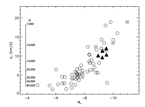
Figure 3.— M_V-$\sigma$ relation for Milky Way GCs (open circles), with data from Pryor & Meylan (1993) and Harris (1996). Training set Milky Way GCs are highlighted in gray squares and the five M31 GCs are shown as filled triangles. Training set and M31 GCs are plotted with reddening corrected V magnitudes and velocity dispersions from Pryor & Meylan (1993). The line width parameter $R$ calculated for a range of velocity dispersions is shown on the inset axis.

Our velocity dispersions, when combined with GC r_h measurements in the literature, allow us to make order of magnitude estimates of the cluster M/L ratios. r_h for all of the GCs in this sample, with the exception of G315, can be found in Barmby et al. (2007). A simple calculation, following Spitzer (1987), assuming the virial theorem and an isotropic velocity distribution for the GCs results in dynamical M/L$\sim$1.5$-$2.5 for these four GCs. Here we have assumed $M=2.5v^{2}r/G$, where $r$, the half-mass radius, is 1.3$\times$r_h, and $v$, the three-dimensional velocity dispersion is $\sqrt{3}\times\sigma$. We can also compare the dynamical M/L to those predicted with population synthesis models. In Percival et al. (2009), the Teramo group provides M/L ratios based on their isochrones and an appropriate IMF from Kroupa (2001). As we use the Teramo isochrones for our abundance analysis (see § 4.2), we can use isochrones which are self-consistent with our later analysis and well-matched to each cluster. Using our own abundance and age constraints, the most appropriate isochrones (ages and metallicities) for our clusters have a M/L$\sim$1.9$-$2.9 based on the Teramo group’s population synthesis work. It is typical to obtain systematically different M/L from dynamical and population synthesis techniques; this difference is probably due to the inclusion of low mass stars in the population synthesis estimate, which are actually ejected in GCs due to dynamical evolution. We find a ratio between dynamical and population synthesis M/L ratios of $0.84\pm 0.27$, which is consistent with the value of $0.73\pm 0.25$ found by Barmby et al. (2007) for a larger sample of M31 GCs. McLaughlin & van der Marel (2005) find a similar ratio of $0.82\pm 0.07$ for a sample of Milky Way and old LMC GCs. These M/L values further identify these four M31 GCs as consistent with the familiar Milky Way GC population.

The relationship described above between light and velocity dispersion is shown in Figure 3. The $\sigma_{obs}$ for Milky Way GCs from Pryor & Meylan (1993), along with absolute magnitudes ($M_{V}$) listed by Harris (1996) are plotted as open circles. For comparison, we also plot the reddening-corrected magnitudes and velocity dispersions from Pryor & Meylan (1993) for our training set GCs as gray squares and those measured for the M31 GC sample as black triangles. From Figure 3 we see that the $\sigma_{obs}$ measured here are consistent with what we would expect given the absolute magnitudes of this set of GCs.

The velocity dispersion that we measure above quantifies another important point about the clusters, which is the limiting resolution that we can obtain for individual spectral lines due to velocity broadening. The velocity dispersions we measure for this set of M31 GCs of 9$-$12 km s^-1  give a line width parameter ($R=\lambda$/FWHM) $R=$14,000$-$10,000, from which it is clear that we are fully sampling the line profiles with the $R=24,000$ spectral resolution provided by the slit configuration used here (the HIRES D3 decker). However, with dispersions this large we expect to have difficulty measuring equivalent widths for elements with weak lines ($\lesssim$30 mÅ), as we discuss in § 5.

Table 4Line Parameters and Integrated-Light Equivalent Widths for M31 GCs

Species	$\lambda$	E.P.	log gf	EW(mÅ)	EW(mÅ)	EW(mÅ)	EW(mÅ)	EW(mÅ)
	(Å)	(eV)		G108	G322	G315	G351	G219
Mg I	4571.102	0.000	$-$5.691	$\cdots$	120.0	$\cdots$	86.7	34.5
Mg I	4703.003	4.346	$-$0.666	$\cdots$	139.2	$\cdots$	99.8	$\cdots$
Mg I	5528.418	4.346	$-$0.341	$\cdots$	$\cdots$	$\cdots$	147.3	58.2
Mg I	5528.418	4.346	$-$0.341	$\cdots$	$\cdots$	$\cdots$	143.6	$\cdots$
Al I	3944.016	0.000	$-$0.638	$\cdots$	$\cdots$	$\cdots$	$\cdots$	134.9
Al I	3944.016	0.000	$-$0.638	$\cdots$	$\cdots$	$\cdots$	$\cdots$	140.1
Si I	7405.790	5.610	$-$0.660	58.4	$\cdots$	$\cdots$	$\cdots$	$\cdots$
Si I	7415.958	5.610	$-$0.730	66.4	$\cdots$	50.1	$\cdots$	$\cdots$
Si I	7423.509	5.620	$-$0.580	84.3	66.5	82.4	$\cdots$	$\cdots$

Note. — Table 4 is presented in its entirety at the end of the text.   Lines listed twice correspond to those measured in adjacent orders with overlapping wavelength coverage.

4. Abundance Analysis

Our new method for obtaining detailed abundances of from their integrated light was developed and tested using a training set of Milky Way and LMC globular clusters. The basic method was described in detail in Bernstein & McWilliam (2002), Bernstein & McWilliam (2005), MB08, and the full training set is presented in S. Cameron et al. (2009) and J. Colucci et al. (2009). The method is briefly summarized below.

4.1. Equivalent Widths and Line Lists

We measure absorption line equivalent widths (EWs) for individual lines in the IL spectra using the semi-automated program GETJOB (McWilliam et al., 1995b), with which we fit low order polynomials to continuum regions and single Gaussian profiles to individual lines and double or triple Gaussians to line blends when necessary. Line lists and oscillator strengths were taken from McWilliam & Rich (1994), McWilliam et al. (1995a), McWilliam (1998), MB08 and Johnson et al. (2006). We measure fewer lines than in standard individual RGB star analyses, as lines in IL spectra are broader and weaker than in individual RGB stars due to the velocity dispersions of the GCs and the presence of continuum flux from warm stars. The lines and EWs included in our final analysis are listed in Table  4. As expected, we find fewer clean lines for the GCs with higher velocity dispersions.

4.2. CMDs and EW Synthesis

In order to synthesize IL EWs to compare to our observed IL EWs, we next need to model the population using theoretical single age, single metallicity isochrones. During analyses of our training set GCs, we performed extensive testing of a variety of isochrones from the Padova (Girardi et al., 2000) and Teramo (Pietrinferni et al., 2004, 2006; Cordier et al., 2007) groups (see MB08, ). Because we require a large, self-consistent parameter space of both scaled-solar and $\alpha-$enhanced isochrones, we have chosen to use the isochrones from the Teramo group for our abundance analyses. The isochrones available cover abundances from Z=0.0001$-$0.04 for both scaled solar and $\alpha-$enhanced ratios. We choose to use the recommended canonical evolutionary tracks including an extended asymptotic giant branch (AGB) and $\alpha-$enhanced low$-$temperature opacities calculated according to Ferguson et al. (2005). We also choose isochrones with mass$-$loss parameter of $\eta$=0.2 because comparison with our training set GCs (particularly those of intermediate metallicity) show that they more accurately match the CMD of GCs; isochrones with $\eta$=0.4 over-predict the fraction of extreme blue horizontal branch (HB) stars at intermediate metallicities. Given that we find blue HB stars are less critical to accurate abundance analysis than red HB stars (see § 6.4), it is more important to our analysis that the isochrones accurately reproduce the red horizontal branch than that they populate the blue region of the horizontal branch when it may be present.

We apply an IMF according to the multiple$-$part power$-$law form described in Kroupa (2002), which changes index at 0.5$M_{\odot}$ and 0.08$M_{\odot}$. Because we only observed the core ($\sim$0.1-0.2$\times$r_h) regions in our training set GCs, we removed stars less massive than $\sim$0.7$M_{\odot}$ from the IMF to match the present day core mass functions (MB08) that have experienced dynamical mass segregation and evaporation of low mass stars (e.g. Baumgardt & Makino, 2003). In this set of M31 GCs we have observed regions corresponding to $\sim$1.5-3r_h, well beyond the core region where significant mass segregation is expected. Although we do expect present day GCs to be stripped of stars less massive than $\sim$0.3$M_{\odot}$ due to dynamical evaporation, the Teramo isochrones stop at 0.5$M_{\odot}$. We do not believe that neglecting stars in the 0.3-0.5$M_{\odot}$ range is a problem for our analysis, as stars less massive than 0.5$M_{\odot}$ contribute only $\sim$1-2$\%$ to the total flux of the population and $<$1$\%$ in absorption features. By combining the model isochrones with cluster-specific IMFs, we can create synthetic CMDs for the range of possible ages and metallicities for which we have isochrones. Each synthetic CMD is divided into $\sim$25 boxes of stars with similar properties, with every box containing $\sim$4% of the total $V$-band flux. The properties of a flux-weighted “average” star in each box are used for the atmospheric parameters needed in synthesizing IL flux-weighted EWs.

Flux-weighted synthesized EWs of lines are calculated using our routine ILABUNDS (see MB08, ) which produces an integrated light EW composed of the $\sim$25 representative stars in each CMD using spectral synthesis routines from MOOG (Sneden, 1973) and model stellar atmospheres from Kurucz (e.g. Castelli & Kurucz, 2004). The synthesized EWs of each of the $\sim$25 representative stars are averaged together, weighted by their respective contribution to the total flux of the cluster. The assumed abundance in the line synthesis is adjusted iteratively until the synthetic flux-weighted EW matches the observed IL EW to 1%. Initial abundance calculations are performed using scaled$-$solar Teramo isochrones and Kurucz ODFNEW stellar atmospheres, and then recalculated with $\alpha$-enhanced Teramo isochrones and AODFNEW atmospheres when abundance results imply enriched $\alpha-$element ratios are present. All five M31 GCs analyzed here were determined to be $\alpha$-enhanced, and thus the abundances we report use $\alpha$-enhanced isochrones and AODFNEW atmospheres in all cases.

All abundances were calculated under the assumption of local thermodynamic equilibrium (LTE). In the case of aluminum we also discuss the non-LTE correction suggested by Baumueller & Gehren (1997) in § 5.3.

Our IL method as implemented here employs a fixed microturbulence law, as described in MB08. Since we do not adjust microturbulence values for individual stars in the synthetic CMDs we must be careful of line saturation. For this reason we only report abundances from lines with EW strengths less than $\sim$150 mÅ for all elements except Fe II. Our analysis indicates that abundances from Fe II lines with EWs over $\sim$100 mÅ start to deviate significantly from the linear portion of the curve of growth. To remain in the linear regime we avoid Fe II lines with EWs $>$100 mÅ wherever possible. In some GCs, like G351-B405, the only clean Fe II lines we measure have EWs $>$100 mÅ. Using these lines in those cases will result in Fe II abundances that may be slightly high. In this work we will refer to lines we do not analyze because of large EWs as “saturated” ($>$150 mÅ  in general, or $>$100 mÅ for Fe II). We note that, in principle, abundance upper limits could be obtained for elements for which all lines are “saturated.” However, due to the flux-weighting of EWs from stars of different types, this analysis requires special care and is not investigated further here.

We have also calculated hyperfine splitting (hfs) abundances for Al, Sc, V, Mn, Co, and Ba. For lines with EWs $>$20$-$30 mÅ, desaturation by hfs can significantly reduce the derived abundances. We use the hfs line lists given in MB08, Johnson et al. (2006), and references therein. Typical hfs abundances corrections here for Al, Sc, V, Mn, Co and Ba were $-$0.1, $-$0.01, $-$0.1, $-$0.4, $-$0.2, and $-$0.15, respectively.

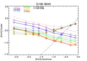
Figure 4.— Fe I (circles) and Fe II (crosses) abundance solutions. The input [Fe/H] value of the isochrone (plotted on the x-axis) equals the output [Fe/H] value of our solution where circles lie on the dashed line.

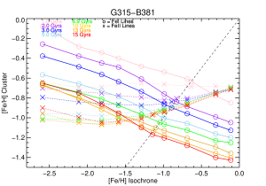
Figure 5.— Same as Figure 4 for G315.

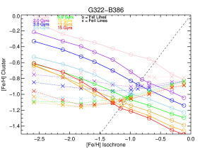
Figure 6.— Same as Figure 4 for G322.

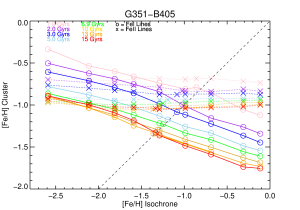
Figure 7.— Same as Figure 4 for G351.

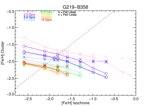
Figure 8.— Same as Figure 4 for G219.

4.3. Finding the Best-Fitting CMD

In the course of our work with the Milky Way and LMC training set GCs, we have explored a variety of strategies for identifying the best-fitting CMD — the CMD which provides abundances that are most consistent with those obtained from the spectral analysis of individual RGB stars in those clusters. Our first efforts to identify the best-fitting CMD focused on obtaining a consistent [Fe/H] solution from the Fe I and Fe II lines. This strategy was discussed with regard to the analysis of 47 Tuc in Bernstein & McWilliam (2002, 2005), and MB08. However analysis of the full training set showed that the Fe I and Fe II lines typically give a self-consistent solution at [Fe/H] values that are frequently more metal-rich than those obtained from analysis of individual stars. There are several possible explanations for a difference in [Fe/H] from Fe I and Fe II lines, although a detailed study of this problem is beyond the scope of this paper. We simply note here that a difference between Fe I and Fe II abundances in individual stars due to non-LTE overionization was noted by (Kraft & Ivans, 2003), and that inaccuracies in Fe II oscillator strengths can lead to large uncertainties in abundances (see recent discussion in Melendez & Barbuy, 2009). These results have led us to focus on a different strategy. Using the training set spectra, we have found that the best-fitting CMD can be consistently identified by taking advantage of the fact that the metallicity dependence of RGB morphology is reasonably well understood (Gallart et al., 2005). After extensive testing, we have found that we obtain consistent, accurate abundances by requiring that the abundance used in calculating the isochrones themselves be consistent with the abundance recovered by our analysis for the Fe I lines. This is consistent with the fact that we find the RGB to have the dominant influence on the strength of the Fe I spectral lines, more so than on the Fe II lines, as discussed in MB08. To clarify our analysis methods, we describe below the procedure we follow for each GC.

For each CMD we calculate a mean [Fe/H] abundance from all available Fe I and Fe II lines. In this data set we measure 30$-$80 Fe I lines and 2$-$10 Fe II lines per GC. Fe abundance results for all CMDs for each GC are plotted in Figures  4 through 8. Circles and crosses correspond to Fe I and Fe II mean solutions. The horizontal axis shows the [Fe/H] of the $\alpha-$enhanced Teramo isochrones. CMDs of the same age are connected by colored lines. Note that $\alpha-$enrichment affects the [M/H] value of the isochrone; for clarity, the value plotted on the x-axis is the true [Fe/H] value rather than the overall metallicity [M/H] (see Pietrinferni et al., 2006).

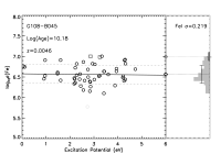
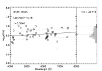
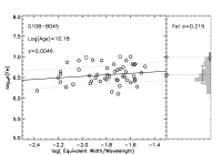
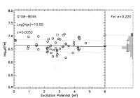
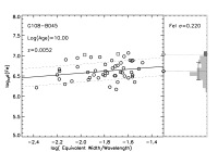
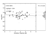
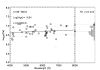
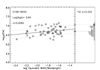
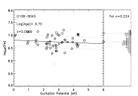
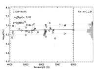
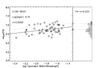
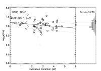
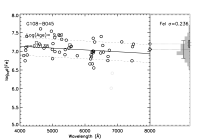
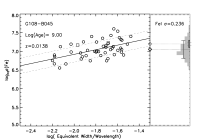
Figure 9.— Diagnostic plots for G108-B045, for ages of 15, 10, 7, 5, and 1 Gyr (top to bottom). Oldest solutions have smallest Fe I standard deviation and smallest dependence on EP, wavelength, or or reduced equivalent width ( log(EW/wavelength)) for this cluster. Fe I and Fe II lines are marked by dark circles and light squares, respectively. Gray points mark lines rejected by a sigma clipping routine when calculating the mean abundances. The solid line shows the linear fit to the Fe I lines and dashed lines show the 1 $\sigma$ deviation of points around the fit. Dark and light diamonds mark the final average Fe I and Fe II abundances.

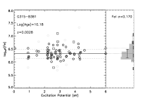
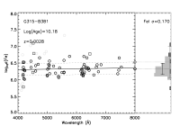
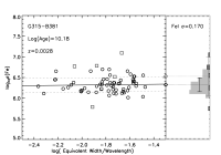
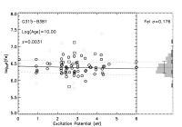
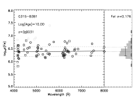
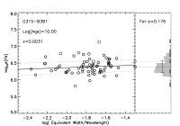
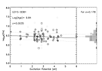
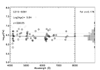
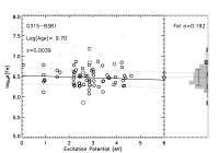
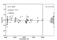
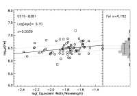
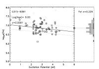
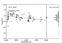
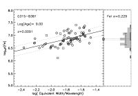
Figure 10.— Diagnostics for G315-B381. The smallest Fe I standard deviation and smallest dependence on EP, wavelength, and observed equivalent width at ages of 10-15 Gyr. Symbols are the same as in Figure 9.

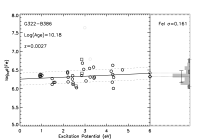
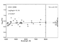
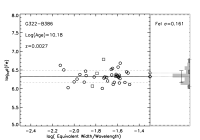
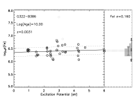
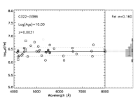
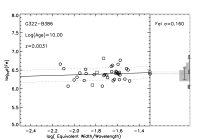
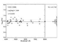
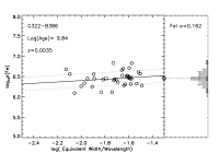
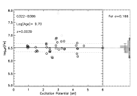
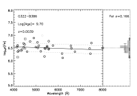
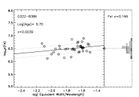
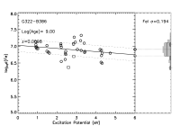
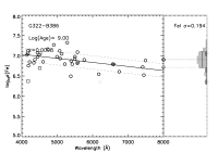
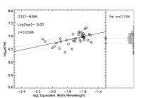
Figure 11.— Diagnostics for G322-B386. The smallest Fe I standard deviation and smallest dependence on EP, wavelength, and observed equivalent width at ages of 7-13 Gyr. Symbols are the same as in Figure 9.

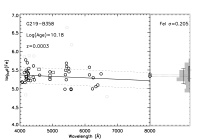
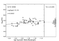
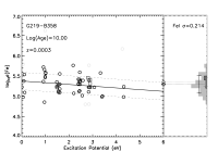
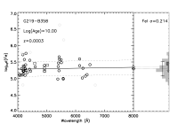
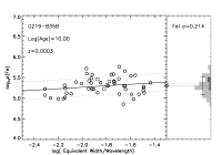
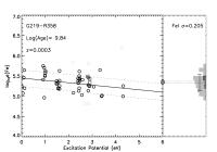
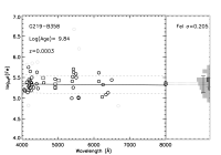
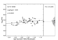
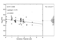
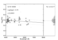
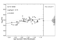
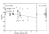
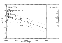
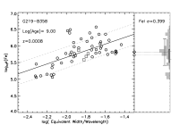
Figure 12.— Diagnostics for G219-B358. The smallest Fe I standard deviation and smallest dependence on EP, wavelength, and observed equivalent width at ages of 7-13 Gyr. Symbols are the same as in Figure 9.

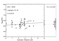
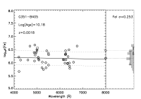
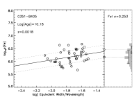
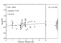
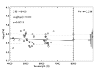
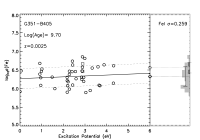
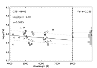
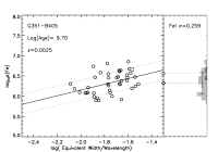
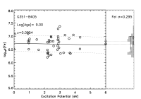
Figure 13.— Diagnostics for G351-B405. The smallest Fe I standard deviation and smallest dependence on EP, wavelength, and observed equivalent width at ages of 10-15 Gyr. Symbols are the same as in Figure 9.

As mentioned above, our criteria for selecting a best-fitting CMD is that the Fe abundance calculated from the Fe I lines is consistent with [Fe/H] used to produce the isochrone. This criteria is met where the solutions cross the dotted black lines in Figures 4 through 8. When the Fe I solution that crosses the dotted line for a given age (color) lies between two isochrones, we interpolate an appropriate isochrone according to the prescription recommended in Pietrinferni et al. (2006). We then have 7 possible solutions where isochrones intercept the dotted black line in Figure 4 — one abundance solution for each age.

We next isolate the best-fitting CMD out of these 7 using diagnostics commonly used in standard stellar abundance analyses. These diagnostics concern the stability of the [Fe/H] solutions, which should not depend on the parameters of the individual line (excitation potentials, wavelengths, or reduced EWs). In principle, as in individual RGB stars, these diagnostics reflect the accuracies in the physical properties of the atmospheres used in the synthesis. The abundance versus excitation potential (EP) diagnostic is sensitive to the temperature of stars, while the abundance versus reduced EW diagnostic is sensitive to the microturbulent velocities of stars. The abundance versus wavelength diagnostic is potentially sensitive to the age of the CMD, because stars of different temperatures dominate the IL flux at different wavelengths. Unlike in RGB stars, in an IL spectrum, correlations with EP and wavelength can be caused by an inaccurate temperature distribution of stars in the CMD, which, for example, could be the result inaccurate modeling of HB morphology in the isochrones. Likewise, correlations with reduced EW can be the result of inaccurate proportions of stars of different gravities as well as a symptom of an inaccurate microturbulent velocity law. These effects are difficult to unravel without additional constraints on the CMD, and identifying these is not the primary goal of this work. We therefore take the existence of any correlations merely as an indication that a given isochrone is less representative of the true CMD then one with weaker correlations. We attempt to identify a best-fitting CMD solution by selecting an isochrone that minimizes these correlations. We use linear least squares fits between [Fe/H] and these parameters to identify and quantify the strength of any existing correlations. Plots illustrating the behavior of the Fe abundances with EP, wavelength, and reduced EW are shown in Figures 9 through 13. From these plots, we obtain 5 diagnostics: the slope of [Fe/H] with EP, wavelength and reduced EW, and the standard deviation of the [Fe/H] solution for Fe I lines and Fe II lines.

For any one of these diagnostics, there is not a statistically significant difference between the quality of the solution from CMDs within a range of $\pm$5 Gyrs. For example, the slope of the [Fe/H] vs. EP relationship in Figure 10 for G315 looks essentially the same for CMDS between ages 5 and 15 Gyrs. However, while the difference in these diagnostics may be small over a wide range in CMD age, we do find that they change monotonically, and are strongly correlated with each other. This suggests that there is clearly a preferred age and [Fe/H] range of CMD for each GC.

To see this more clearly, we plot these diagnostics for the M31 sample in Figures 14 through  18. These plots show all five diagnostics as a function CMD age for the 7 CMDs that satisfy the original selection criteria (see Figures 4 through 8). From Figures 14 through  18, it is clear that for all of the GCs in our sample, all five diagnostics simultaneously imply that better solutions are obtained for CMDs with ages $>$7 Gyr. For these GCs, as for old Milky Way GCs analyzed as part of our training set (S. Cameron et al. 2009), we find the acceptable CMD ages typically cover a range of 5 Gyrs (e.g. 10$-$15 Gyrs or 7$-$13 Gyrs). This is not surprising because the CMDs themselves change very little over those ranges in age. We discuss these age constraints in detail in the next section.

From this range of acceptable ages, we select one CMD to use for a final analysis run of all elements for which we measure lines. For old GCs, such as the present sample, our abundance results are quite insensitive to which CMD in this age range is used. Again, this is not surprising as the CMDs in this age range are very similar. This weak dependence is quantified in Figure 19, in which the upper plot shows the small difference in abundance between the oldest and youngest CMDs in the acceptable age range for each GC (discussed in § 5.1). Nearly all elements change by $\leq$0.1 dex, and older CMD ages always give smaller abundances. The lower plot of Figure 19 demonstrates that the derived abundance ratios are even more robust. Since the change in the abundances of most elements tracks the change in Fe, the net difference in the abundance ratios is $<$0.05 dex in almost all cases.

Figure 14.— Fe line abundance diagnostics for G108. All diagnostics are normalized to their maximum values so that they can be shown on the same scale. The thick black line is Fe I $\sigma$, thick dashed orange line is Fe II $\sigma$, dotted blue line is the slope in [Fe/H] vs. $\lambda$, thin dashed green line is the slope in [Fe/H] vs. reduced EW, and the thin red solid line is the slope in [Fe/H] vs. EP.

Figure 15.— Same as Figure 14 for G315.

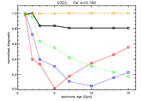
Figure 16.— Same as Figure 14 for G322.

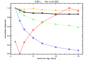
Figure 17.— Same as Figure 14 for G351.

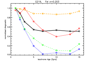
Figure 18.— Same as Figure 14 for G219.

5. Results: Chemical Abundances

We have measured abundances from the available clean lines of $\alpha-$elements, Fe and Fe$-$peak elements, and neutron capture elements for each GC. Final abundances, the number of analyzed spectral lines, line-to-line scatter, and the age of the best-fitting isochrone are reported in Tables 5 through 9. All abundance ratios relative to Fe use the solar abundance distribution of Asplund et al. (2005), with a solar log$\epsilon$(Fe)$=7.50$. Abundance ratios of Sc II, Ti II, Y II, and Ba II are reported with respect to [Fe/H]_II. Figures 20 through 24 show the M31 abundance ratios (green circles) compared to our Milky Way training set IL abundances (red squares). Error bars for IL abundances in Figures 20 through 24 correspond to the statistical error of the deviation in abundances from the N_lines available for each species, as reported in Tables 5 through 9. Note that these errors are often larger for the Milky Way training set abundances, which is a result of the smaller luminosity sampling of these GCs (5-30 % of the total flux) and, in some cases, lower SNR spectra.

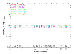
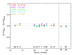
Figure 19.— Robustness of the abundances over the $\sim$5 Gyr range of acceptable isochrone ages. Top plot shows the difference in the log$\epsilon$(X) of older and younger solutions. Bottom plot shows the corresponding difference in abundance ratios. Dotted lines around zero mark a change of $\pm$ 0.1 dex.

5.1. Iron and Ages

As in abundance analyses of individual stars, the first element we analyze is Fe because the large number of available transitions provide a wide variety of very useful diagnostics and consistency checks. As outlined in § 4.3, we first use the Fe lines to constrain our best CMDs. We find this sample of M31 GCs is old, with preferred ages $>$7 Gyrs, which is consistent with age estimates from previous photometric and low resolution spectroscopic work (Rich et al., 2005; Huchra et al., 1991). We also find this sample of GCs spans a metallicity range of [Fe/H]$\sim-0.9$ to $-2.2$, which is within the range of [Fe/H] of Milky Way GCs system. Below, we briefly discuss the best age and [Fe/H] for the individual GCs in this sample.

We find the preferred range of CMD ages for G108 to be 10-15 Gyrs. We pick a best CMD age of 15 Gyrs for our final abundance determinations. For the best solutions we find negligible trends of Fe I abundance with EP and a slight correlation remaining with wavelength and reduced EW, as shown in Figure 9. We note that the remaining correlation between Fe abundance and reduced EW suggests that the microturbulent velocity law we have applied is not perfect for every star in the synthetic CMD. However, while the correlation may still be present in the best solution, the overall trend in correlations over all CMDs is still very clear, and it is easy to select the most appropriate CMD. It is important to note that the scatter in microturbulence values around the relation we have adopted is at least $\pm 0.2$ km s^-1  for studies of both dwarf and RGB stars in the Milky Way (e.g. Bensby et al., 2005; Fulbright et al., 2006). We have experimented with adjusting the microturbulence law within this range, which could potentially reduce the Fe abundance standard deviation. However, as long as the dependence of Fe abundance on reduced EW is small, this will not significantly alter the mean Fe abundance. We have not been able to find a microturbulence law that improves the overall abundance solution (i.e. improves all five diagnostics discussed in § 4.3). A more detailed investigation of this issue is beyond the goals of this study. To preserve the self-consistency of our solutions between GCs, we do not alter the original microturbulent velocities of the best-fitting CMD. A detailed discussion of the small ($<$0.1 dex) systematic error between the IL spectra abundance analysis and that for individual stars is included in S. Cameron et al. (2009). For the purposes of this work, we avoid systematic error issues by concentrating on relative comparisons between IL abundances determined in the same way for M31 and Milky Way GCs in our training set. To summarize our results, the final abundance solution for G108 is [Fe/H]$=-0.94\pm 0.03$, where the uncertainty is the standard error in the abundances from all Fe lines ($\sigma/\sqrt{N_{lines}-1}$).

The preferred CMD age range for G315 is also 10-15 Gyrs. Four of the five diagnostics show best solutions at the oldest ages, therefore we use the 15 Gyr solution as our best CMD. The 15 Gyr solution for G315 has negligible trends of Fe I abundance with EP, wavelength, and reduced EW, which can be seen in Figure 10. The final abundance for G315 is [Fe/H]$=-1.17\pm 0.02$.

As can be seen in Figures 11 and 16, for G322 we find the EP correlation to be slightly stronger at the oldest ages, resulting in a slightly younger preferred age range of 7-13 Gyrs. We use a best CMD age of 13 Gyrs, and find a negligible correlation with wavelength and reduced EW, but a slight correlation between Fe abundance and EP for this solution. The final abundance is [Fe/H]$=-1.14\pm 0.03$.

G219 is the only GC in this sample which appears to be slightly younger than the others. Figure 18 shows that four out of five Fe line diagnostics are best for ages of 7-13 Gyrs. We pick a best CMD age of 10 Gyrs, which is in the middle of this preferred age range. Figure 12 shows that this best solution —the 10 Gyr CMD— still shows slight correlations of Fe abundance with EP and reduced EW. We find an [Fe/H]=$-2.21\pm 0.03$ for G219, which makes it one of the most metal-poor GCs in the Local Group confirmed by high resolution spectra to date.

The preferred CMD age for G351 is 10-15 Gyrs. We note that G351 has a larger Fe I standard deviation than any other GC in the sample for any solution, which can be seen in Figure 13. We choose a best CMD age of 15 Gyrs, and note that this solution has small correlations of Fe abundance with EP and wavelength, as well as a fairly significant correlation with reduced EW. We find [Fe/H]$=-1.33\pm 0.04$.

Table 5G108-B045 Abundances

Species	log${}_{10}\epsilon($X$)$	$\sigma$	Error	[X/Fe]	$N_{lines}$
	15 Gyrs
Si I	7.15	0.17	0.12	$+$0.58	3
Ca I	5.64	0.17	0.07	$+$0.26	7
Sc II	2.54	0.26	0.18	$-$0.00	3
Ti I	4.10	0.21	0.10	$+$0.14	5
Ti II	4.86	0.34	0.17	$+$0.47	5
V I	2.90	0.24	0.17	$-$0.16	3
Cr I	4.82	$\cdots$	$\cdots$	$+$0.12	1
Mn I	4.05	0.15	0.09	$-$0.40	4
Fe I	6.56	0.22	0.03	$-$0.94	49
Fe II	6.99	0.01	0.01	$-$0.51	2
Co I	4.30	0.19	0.13	$+$0.32	3
Ni I	5.47	0.27	0.14	$+$0.18	5
Y II	1.45	$\cdots$	$\cdots$	$-$0.25	1

Table 6G315-B381 Abundances

Species	log${}_{10}\epsilon($X$)$	$\sigma$	Error	[X/Fe]	$N_{lines}$
	15 Gyrs
Si I	7.01	0.27	0.27	$+$0.67	2
Ca I	5.51	0.18	0.07	$+$0.37	9
Sc II	2.29	0.38	0.22	$+$0.21	4
Ti I	4.07	0.15	0.11	$+$0.34	3
Ti II	4.53	0.30	0.15	$+$0.60	5
V I	2.72	$\cdots$	$\cdots$	$-$0.11	1
Cr I	4.63	0.15	0.15	$+$0.16	2
Mn I	3.75	0.14	0.08	$-$0.47	4
Fe I	6.33	0.17	0.02	$-$1.17	61
Fe II	6.53	0.50	0.19	$-$0.97	6
Ni I	4.97	0.19	0.09	$-$0.09	6
Y II	1.44	$\cdots$	$\cdots$	$+$0.20	1
Ba II	1.45	$\cdots$	$\cdots$	$+$0.25	1

Table 7G322-B386 Abundances

Species	log${}_{10}\epsilon($X$)$	$\sigma$	Error	[X/Fe]	$N_{lines}$
	13 Gyrs
Mg I	6.70	0.08	0.08	$+$0.35	2
Si I	6.70	$\cdots$	$\cdots$	$+$0.272	1
Ca I	5.46	0.16	0.06	$+$0.33	8
Ti I	4.21	0.14	0.10	$+$0.49	3
Ti II	4.33	0.21	0.12	$+$0.51	4
V I	3.02	$\cdots$	$\cdots$	$+$0.20	1
Cr I	4.68	$\cdots$	$\cdots$	$-$0.043	1
Mn I	3.61	0.07	0.05	$-$0.60	3
Fe I	6.36	0.16	0.03	$-$1.14	35
Fe II	6.43	0.41	0.21	$-$1.07	3
Ni I	5.15	0.26	0.19	$+$0.10	3
Ba II	1.63	$\cdots$	$\cdots$	$+$0.54	1

Table 8G219-B358 Abundances

Species	log${}_{10}\epsilon($X$)$	$\sigma$	Error	[X/Fe]	$N_{lines}$
	10 Gyrs
Mg I	5.42	0.14	0.14	$+$0.09	2
Al I	4.24	0.05	0.05	$+$0.692	2
Ca I	4.49	0.14	0.05	$+$0.39	8
Sc II	0.95	$\cdots$	$\cdots$	$+$0.05	1
Ti II	3.33	0.22	0.13	$+$0.58	4
Cr I	3.28	0.29	0.12	$-$0.15	7
Fe I	5.29	0.21	0.03	$-$2.21	47
Fe II	5.35	0.12	0.05	$-$2.15	4
Ba II	0.04	0.08	0.04	$+$0.02	4

5.2. Alpha Elements

As described in § 1, [$\alpha$/Fe] abundance ratios are a valuable tool for studying the star formation history of a galaxy. $\alpha-$elements are produced primarily in SNII that occur on timescales of 1-20 million years, which corresponds to the lifetimes of massive stars. While Fe-peak elements are produced in both type Ia (SNIa) and SNII, the SNIa contribution dominates on timescales of $\gtrsim$10⁹ years (e.g. Smecker-Hane & Wyse, 1992). Thus, at early times many $\alpha-$elements are produced while total Fe abundances are low, resulting in an enhanced [$\alpha$/Fe] abundance ratio at low [Fe/H]. After the onset of SNIa, the total Fe abundance increases at a faster rate than that of $\alpha-$elements, decreasing the [$\alpha$/Fe] ratio (Tinsley, 1979). Most GCs in the Milky Way have [$\alpha$/Fe] ratios that are enhanced with respect to solar abundance ratios, similar to Milky Way halo stars at comparable [Fe/H]. This implies that Milky Way GCs formed when the ISM was dominated by enrichment by SNII. Like Milky Way GCs, we find all the GCs in our M31 sample to be enhanced in Ca, Ti and Si.

Abundances for Ca I come from 7$-$9 clean lines per GC, with rms scatter about the mean of 0.1$-$0.2 dex, which is similar to the scatter in our Fe abundances. We measure 4$-$10 Ti I and Ti II lines per GC, with slightly higher line-to-line scatter that may be due to weak blends. We are able to confidently measure 1$-$3 Si I lines in three of the GCs; lines in G219 and G351 were too noisy or badly blended to use. The one Si I line we measure in G322 is partially blended. To estimate the effect of weak blends on the Si abundance from the EW, we have used the SYNTH routine from MOOG, which we have modified to synthesize IL spectra. We estimate that at most our EW abundance measurement is $\sim$0.1 dex too high after visual inspection of synthesized IL spectra of different abundances.

In Milky Way field stars, the [Mg/Fe] ratios behave similarly to Ca, Ti and Si. However, in Milky Way GCs, [Mg/Fe] shows inter- and intra-cluster abundance variations (see Gratton et al., 2004) with respect to other $\alpha-$elements and star-to-star differences within individual GCs. Analysis of our full training set of Milky Way GCs has revealed lower [Mg/Fe] than [Ca/Fe], [Ti/Fe], or [Si/Fe] in three out of the six GCs where it was measured (see MB08 and Cameron et al. 2009).

We have been able to measure [Mg/Fe] in three of the GCs in M31. Similar to the Milky Way training set GCs, in M31 we measure [Mg/Fe] to be lower ( [Mg/Fe]$<+$0.1 dex) than other $\alpha-$elements within individual GCs in two out of the three GCs where it was measured. In the other two clusters the Mg I lines had strengths $>$ 150 mÅ, and were therefore not analyzed in this work.

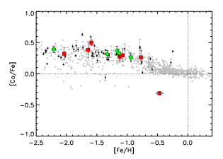
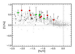
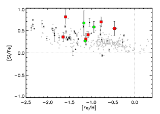
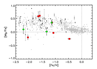
Figure 20.— $\alpha-$element ratios. Gray points show Milky Way Stars and black points show mean Milky Way GCs abundances from single stars. Data for single stars is from Venn et al. (2004), Pritzl et al. (2005) and references therein. When possible, these abundance ratios have been adjusted to be consistent with the solar abundance distribution of Asplund et al. (2005) that was used in our analysis. Red squares show the abundances from our Milky Way training set ILS analysis and green circles show M31 ILS abundances. The average of [Ti/Fe]_I and [Ti/Fe]_II are plotted vs. [Fe/H]_I, where we have measured them.

We have performed spectral synthesis tests of the Mg I lines to see if the [Mg/Fe] depletion can be explained by line-to-line measurement error. An example of this test is shown in Figure 25, for the unblended 5528 Å Mg I line in the most metal-poor GC G219. From the EW of this line, we measure an abundance of [Mg/Fe]$=+0.01$. Overplotted are synthesized spectra with abundances of [Mg/Fe]$=+0.3,0.0,-0.3$. G219 is extremely metal poor, and no other elements contribute to the line EW. It is clear from Figure 25 that the closest matching abundance is [Mg/Fe]$=0.0$, and that the line is inconsistent with the [$\alpha$/Fe]$=+0.3$ measured for Ca and Ti, clearly showing that measurement error cannot explain the Mg deviation from the other $\alpha$-element abundances in this cluster. In § 6.2, we further discuss light element variations in the IL of GCs, and in § 6.3.2 we discuss further implications for low resolution IL abundances.

Table 9G351-B405 Abundances

Species	log${}_{10}\epsilon($X$)$	$\sigma$	Error	[X/Fe]	$N_{lines}$
	15 Gyrs
Mg I	6.22	0.22	0.13	$+$0.01	4
Ca I	5.30	0.16	0.06	$+$0.32	9
Sc II	1.67	$\cdots$	$\cdots$	$-$0.34	1
Ti I	3.94	0.40	0.23	$+$0.37	4
Ti II	4.49	0.25	0.25	$+$0.62	2
Cr I	4.44	$\cdots$	$\cdots$	$-$0.132	1
Mn I	3.49	$\cdots$	$\cdots$	$-$0.57	1
Fe I	6.17	0.26	0.04	$-$1.33	42
Fe II	6.46	0.17	0.10	$-$1.04	2
Ni I	$\cdots$	$\cdots$	$\cdots$	$-$0.23	1
Ba II	1.39	0.29	0.20	$+$0.26	3

Table 10Mean IL $\alpha$ Abundances for Milky Way Training Set and Current Sample of M31 GCs

	Milky Way	M31
$[$Ca/Fe$]$	$+$0.35 $\pm$ 0.08	$+$0.34 $\pm$ 0.05
$[$Ti/Fe$]$	$+$0.46 $\pm$ 0.15	$+$0.47 $\pm$ 0.10
$[$Si/Fe$]$	$+$0.52 $\pm$ 0.20	$+$0.51 $\pm$ 0.21
$[$Mg/Fe$]$	$+$0.18 $\pm$ 0.39	$+$0.15 $\pm$ 0.17
$[$$\alpha$CaTiSiMg/Fe$]$	$+$0.38 $\pm$ 0.15	$+$0.37 $\pm$ 0.16
$[$$\alpha$CaTiSi/Fe$]$	$+$0.44 $\pm$ 0.09	$+$0.44 $\pm$ 0.09

We can address the star formation history of M31 by calculating an average [$\alpha$/Fe] ratio for each GC similar to that in Pritzl et al. (2005). While these authors use Ca, Ti, Si, and Mg in their average [$\alpha$/Fe], we note that [Mg/Fe] is probably not a good [$\alpha$/Fe] indicator in the IL of GCs, for the reasons discussed above. Therefore, for the mean [$\alpha$/Fe] for each GC discussed here, we include only Ca I, Ti I, Ti II, and Si I. The mean [$\alpha$/Fe]$=+0.36\pm 0.20$, $+0.50\pm 0.16$, $+0.40\pm 0.12$, $+0.44\pm 0.16$, and $+0.49\pm 0.13$ for G108, G315, G322, G351 and G219, respectively, which is significantly and consistently enhanced relative to solar in all five M31 GCs. We can also calculate the mean ratio for the individual $\alpha-$elements across the sample of GCs, and compare these values to similar means in our sample of Milky Way training set GCs. This comparison of abundances derived only with our IL spectra method avoids any potential sources of systematic error. The mean values for Ca, Ti, Si, and Mg are presented in Table 10. In addition, we present the mean and deviation of all the [$\alpha$/Fe] ratios including and excluding [Mg/Fe]. Table 10 shows that GCs in both the Milky Way and M31 have extremely consistent [$\alpha$/Fe] ratios. GCs in both galaxies are also consistent with the Milky Way halo average $\alpha$-enhancement of $+0.35$ (e.g. McWilliam, 1997). The obvious implication of the [$\alpha$/Fe] abundances in this small sample of M31 GCs is that M31 was (or its now-merged components were) dominated by enrichment by SNII when these GCs formed.

5.3. Aluminum

Al abundances have been used to put constraints on chemical evolution models of the Milky Way because Al enrichment is particularly sensitive to the details of SNII explosions (see Gehren et al., 2006). Al abundances for Milky Way disk stars with [Fe/H]$<-2$ have some contribution from explosive burning in SNII (Andrievsky et al., 2008), so that like [$\alpha$/Fe], Al abundances reach a plateau value of [Al/Fe] $\sim+0.3$ (e.g. Bensby et al., 2005). However, some stars in Milky Way GCs are found to be even more enriched, reaching levels as high as [Al/Fe]$\sim+1$ (Gratton et al., 2001). Also, like Mg, Al exhibits inter- and intra-cluster variations, which we discuss further in § 6.2, suggesting that the influences on Al abundance are more complicated in GCs than in the field.

We have only been able to make one measurement of Al I in this first sample of M31 GCs. This measurement was made from the 3944 Å Al I line in the metal-poor GC G219. We were able to make two independent measurements of this 3944 Å line because it was present at the ends of two adjacent orders. Both measurements give a consistent result of [Al/Fe]$=+0.09\pm 0.05$. However, we note that Al I abundances derived from the 3944 Å resonance line can be problematic; McWilliam et al. (1995a) find that the line is significantly blended with CH lines in some giant stars, which causes derived abundances to be too high, and according to Baumueller & Gehren (1997) Al I abundances from this line will be underestimated by $\sim$0.6 dex due to non-LTE effects. Andrievsky et al. (2008) find that this correction may be even larger in metal-poor hot stars. We do not see evidence in the IL spectrum for contamination of the 3944 Å line by significant CH blends. An appropriate non-LTE correction of $+0.6$ dex raises the abundance to [Al/Fe]$=+0.69$. This is higher than the [Al/Fe]$\sim$0 halo average at an [Fe/H]=$-2.2$, but consistent with the significantly enhanced Al I found in some individual GC stars. This enhanced [Al/Fe] is also consistent with Al abundances we derive for three Milky Way GCs in our training set.

The training set [Al/Fe] measurements provide much stronger evidence that the enhanced [Al/Fe] we measure in GC IL spectra is real because they are not measured from the potentially problematic 3944 Å Al I feature. The training set [Al/Fe] (see Figure 21) were measured from the 6696/6698 Å Al I doublet, which should not be contaminated by blends. In addition, Baumueller & Gehren (1997) find that non-LTE effects are much smaller for these lines. The 6696 Å feature is not detectable in G219, even though we measure an abundance as high as [Al/Fe]$=+0.7$ with the non-LTE correction. We performed spectral synthesis tests to check that the lower limit of [Al/Fe]$=+0.7$ is consistent with a 6696 Å line that would be too weak to detect in the IL spectra. We indeed find that an [Al/Fe]$=+0.7$ is not high enough for the feature to be seen after convolution with the velocity broadening of G219 because it results in a line depth of $<0.01\%$ of the continuum level.

The 6696/6698 Å features were also too weak in the other M31 GC spectra to get reliable abundance measurements from EWs, with the exception of G108, in which it unfortunately falls too near the end of an order for a good measurement to be made. The 3944 Å line was saturated in all of the more metal-rich GCs.

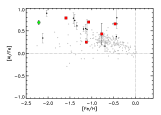
Figure 21.— Aluminum abundances. Symbols are the same as in Figure 20. GC data is from references compiled in Carretta (2006). A non-LTE correction of 0.6 dex has been added to G219 abundance.

5.4. Fe-peak Elements

Ni, Cr, Mn Co, Sc, and V abundances are interesting because their production generally tracks that of Fe, (e.g. Iwamoto et al., 1999), resulting in [X/Fe]$\sim 0$. Therefore, deviations from [X/Fe]$\sim 0$ are particularly interesting because they imply special conditions may have been present, such as variations in the mass function of supernovae, variations of mixing of supernovae ejecta into the local ISM, metallicity dependent or explosion dependent supernova yields, or contributions from special types of supernovae (e.g. McWilliam, 1997).

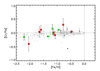
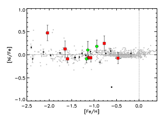
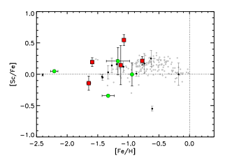
Figure 22.— Abundances for Fe peak elements Cr, Ni and Sc. Symbols are the same as Figure 20. GC data from Kraft et al. (1995), Sneden et al. (1997), Cohen et al. (1999), Ivans et al. (1999), Shetrone & Keane (2000), Ivans et al. (2001), Ramírez & Cohen (2002), Lee & Carney (2002), Sneden et al. (2004), Carretta et al. (2004), Cohen (2004), Tautvaišienė et al. (2004), and Lee et al. (2005)

Ni abundances in Milky Way field and GC stars generally follow the expected Fe-peak element trend of [Ni/Fe]$=0$ at all metallicities. We are able to measure [Ni/Fe] in three M31 GCs, and find it to be consistent with the Milky Way abundance trend. Ni was measured from 3-6 Ni I lines in G108, G315, and G322. The three GCs have a mean $<$[Ni/Fe]$>=+0.06\pm 0.14$, which is essentially identical to the mean of the Milky Way training set GCs, which have $<$[Ni/Fe]$>=+0.05\pm 0.21$.

In the most metal-poor cluster G219, all Ni I lines are too weak for EWs to be measured reliably. In G315 most Ni I lines are too weak or noisy for EW measurements, and the 7393 Å line is blended with telluric absorption lines. We estimate from spectral synthesis tests of the noisy 6767 Å line in G351, that [Ni/Fe]$\sim-0.2$. The spectral synthesis and spectrum are shown in Figure 26, where the uncertainty in abundance due to the noisy continuum can be fully appreciated.

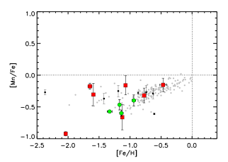
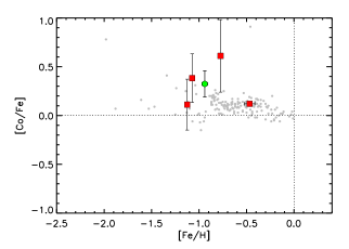
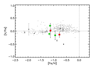
Figure 23.— Abundances of Mn, Co and V. Symbols and references are the same as Figure 22.

[Cr/Fe]$=0$ in Milky Way stars for [Fe/H]$>-2$, but [Cr/Fe]$<0$ for [Fe/H]$<-2$. The deviation from [Cr/Fe]$=0$ at low metallicity may be due to different chemical enrichment for the lowest metallicity stars in the Milky Way halo (McWilliam, 1997). We measure Cr I abundances for the four most metal-rich M31 GCs that are consistent with the solar [Cr/Fe] average in both our Milky Way training set GCs and in Milky Way stars at these metallicities. Few [Cr/Fe] measurements exist for GCs with [Fe/H]$<-2$. When observed, [Cr/Fe] in GCs also follows the decreasing [Cr/Fe] abundance trend observed in Milky Way halo stars (see Shetrone et al. (2001) for M92 and NGC 2419, and Letarte et al. (2006) for M15 and Fornax GCs). We are able to measure Cr I in the low-metallicity M31 cluster G219, and find [Cr/Fe]$=-0.15$, which is also consistent with the decreasing halo abundance trend below [Fe/H]$\sim-2$. Cr abundances were calculated from one Cr I line in G108, G322 and G351, two Cr I lines in G315, and seven Cr I lines in G219. Most other Cr I lines in the more metal-rich GCs have EWs over 150 mÅ and were not analyzed. The Cr feature at 5409 Å, which is the only Cr line we measure in G322 and G351, is partially blended with weak Ti I and Fe I lines, so that the EW abundance may be slightly high. We used spectral synthesis tests of the Ti I and Fe I blends around the 5409 Å Cr I feature to estimate the effect of the blends on the derived Cr abundance. We find that the Cr I abundance derived with the original EW measurement may be approximately $\sim$0.25 dex too high. A correction of $-0.25$ dex to our EW abundances of [Cr/Fe]$=+0.21$ and $+0.12$, would result in [Cr/Fe]$=-0.04$, and $-0.13$ for G322 and G351, respectively. These [Cr/Fe] are consistent with the [Cr/Fe]$\sim 0$ of Milky Way GCs.

Mn is a particularly interesting Fe$-$peak element because unlike most Fe$-$peak elements the [Mn/Fe] ratio is not solar at most metallicities. From [Fe/H]$=-1$ to $-2.5$ dex, [Mn/Fe]$\sim-0.4$, and increases to [Mn/Fe]$=0$ at [Fe/H]$=0$. This trend is similar but opposite to that of $\alpha-$elements (e.g. McWilliam, 1997). Possible explanations for this trend are: Mn is underproduced in SNII and overproduced in SNIa, or that SNIa Mn production is dependent on the metallicity of the progenitor star (Gratton, 1989). Recent observations of [Mn/Fe] in stars in the Sagittarius Dwarf Galaxy have shown that only the latter explanation can simultaneously reproduce the data in both the Milky Way and Sagittarius (McWilliam et al., 2003; Cescutti et al., 2008). This demonstrates the importance of obtaining abundance ratios in a variety of environments for a full understanding of chemical evolution. Because Bergemann (2008) find that Mn abundances may be underestimated due to non-LTE effects over most of this metallicity range, we focus on a relative comparison of our abundances with others calculated under similar assumption of LTE.

We find that the Mn I abundances in the M31 GCs are consistent with our training set abundances and the Milky Way [Mn/Fe] abundance trend. Our abundances for Mn are measured from 3$-$4 Mn I lines in each the three most metal-rich GCs, G108, G315 and G322. [Mn/Fe] is measured from the Mn I 6021 Å line only in G351. We do not see evidence for blends that would change the result by more than $\sim$0.1 dex.

The mean [Sc/Fe] in Milky Way stars and GCs is approximately solar. We measure a mean [Sc/Fe]$\sim 0$ for GCs in M31, with a larger scatter between lines for individual GCs and between the five GCs ($\sigma\sim 0.2$ dex) than we see for other, easier-to-measure Fe$-$peak elements ($\sigma\sim 0.1$). We find a similar mean and scatter in our training set GC abundances. We measure abundances for 1$-$4 Sc II lines in each of the five GCs.

Co abundances in stars and GCs in the Milky Way track that of Fe for [Fe/H]$>-2$, so that over this range in metallicity the [Co/Fe]$\sim 0$. We measure Co I from three lines for the most metal-rich GC G108. Co I features in the other four GCs are too weak to measure reliably, with the exception of the feature at 4121 Å, which we find to be significantly blended. The G108 [Co/Fe]$=+0.32\pm 0.13$ is in agreement with Milky Way training set abundances at this metallicity.

Milky Way stellar and GC V abundances typically track the abundance of Fe, resulting in [V/Fe]$\sim 0$. We measure a mean V abundance from G108, G315, and G322 of [V/Fe]$=-0.02$, which is consistent with our measurements of [V/Fe] in the Milky Way training set GCs. Abundances for G108 come from 3 V I lines, and abundances for G315 and G322 each come from the V I 6081 Å line. These V I lines are all weak (EWs$\sim$30-40 mÅ), but it appears unlikely that there are any blends that would cause misleading abundance measurements.

In summary, the Fe-peak element abundances in this sample of M31 GCs are similar to those measured in Milky Way GCs, and consistent with enrichment dominated by SNII.

5.5. Neutron Capture Elements

The relative abundances of neutron capture elements are important because they are particularly sensitive to the details of star formation, but also because the nucleosynthetic sources and yields of the rapid ($r-$process) and slow ($s-$process) neutron capture reactions remain uncertain (see Venn et al., 2004; McWilliam, 1997). In particular, the difference between the Ba and Y abundances for stars in the Milky Way and stars in nearby dwarf spheroidal galaxies provides strong evidence for differences between the star formation histories of large galaxies and their satellites (Shetrone et al., 2001, 2003; Geisler et al., 2005). Perhaps more interesting is that these abundance differences are at times inconsistent with simple nucleosynthetic explanations, and thus can provide new constraints on uncertain reaction sites (e.g. Venn et al., 2004).

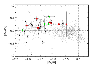
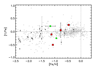
Figure 24.— Abundances of neutron capture elements. Symbols and references are the same as in Figure 20.

We are able to measure abundances for the strong lines of Ba II and Y II in some of the M31 GCs. Unfortunately, we are unable to measure abundances for weaker Eu II and La II lines due to the high velocity dispersions of this sample of GCs (see § 3). Typical Ba abundances in Milky Way GC stars are between [Ba/Fe]$\sim 0-0.5$ for [Fe/H]$>-1$ and [Ba/Fe]$<0$ for [Fe/H]$<-1$. Our Ba abundances for the M31 GCs are consistent with these trends and with what we find for our training set GCs; we also measure the lowest [Ba/Fe] for the lowest metallicity cluster G219. Ba II abundances come from 1-4 lines in each of the GCs except for the most metal-rich cluster G108, for which all line strengths were over 150 mÅ.

For [Fe/H]$>-1.5$, Milky Way GCs typically have [Y/Fe]$\sim 0$. We measure a mean value of [Y/Fe]$\sim 0$ for G108 and G315 in M31, as well, which is also consistent with what we find for the Milky Way training set. These Y abundances come from the 4883 Å Y II feature. Because the Y abundances are derived from a single line, we have performed spectral synthesis tests to confirm that the 4883 Å line is relatively unaffected by blends.

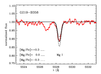
Figure 25.— Spectrum synthesis test for Mg I 5528 Å line in G219. Smoothed data is shown in red, and overplotted synthesized spectra from top to bottom correspond to [Mg/Fe]$=-0.3,0.0,+0.3$. The closest matching profile is for [Mg/Fe]$=0.0$.

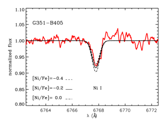
Figure 26.— Spectrum synthesis test for Ni I 6767 Å line in G351. Smoothed data is shown in red, and overplotted synthesized spectra from top to bottom correspond to [Ni/Fe]$=-0.4,-0.2,0.0$. The spectrum is noisy and continuum placement uncertain, but [Ni/Fe] is approximately $\sim-0.2$ with an uncertainty of $\sim$0.2 dex.

6. Discussion

Table 11Metallicity Comparisons

	ILS	1	2	3	4
Cluster	[Fe/H]	[Fe/H]	[Fe/H]	[Fe/H]	[Fe/H]
G108-B045	$-$0.94 $\pm$ 0.03	$-$0.85	$-$0.94 $\pm$ 0.27	$-$1.05 $\pm$ 0.25	$-$0.71 $\pm$ 0.11
G219-B358	$-$2.21 $\pm$ 0.03	$-$1.92	$-$1.83 $\pm$ 0.22	$\cdots$	$-$2.00 $\pm$ 0.11
G315-B381	$-$1.17 $\pm$ 0.02	$\cdots$	$-$1.22 $\pm$ 0.43	$\cdots$	$\cdots$
G322-B386	$-$1.14 $\pm$ 0.02	$-$1.09	$-$1.21 $\pm$ 0.38	$-$1.62 $\pm$ 0.14	$-$1.03 $\pm$ 0.22
G351-B405	$-$1.33 $\pm$ 0.04	$-$1.77	$-$1.80 $\pm$ 0.31	$\cdots$	$\cdots$

References. — From CMD photometry: (1.) Rich et al. (2005). From Lick index spectroscopy: (2.) Huchra et al. (1991) (3.) Perrett et al. (2002) (4.) Puzia et al. (2005), calculated from the relation in Thomas et al. (2003) : [Fe/H]$=$[Z/H]$-0.94$[$\alpha$/Fe].

Although this is only the first set in a larger sample of GCs from our M31 study, we already have several interesting results. First, in § 6.1 we discuss the chemical enrichment history of the present sample of M31 GCs and compare it to the Milky Way and dwarf galaxy GC systems. In § 6.2 and § 6.3 we discuss the implications of our measurements for both GC formation and evolution and IL abundance work at low resolution. In the final two sections we comment on constraints that can be put on horizontal branch morphology and reddening of unresolved GCs using high resolution IL spectra.

6.1. Chemical History of M31 GCs

Overall, these five M31 GCs are old and have chemical properties similar to those of most Milky Way GCs. All five GCs are enhanced in the $\alpha-$elements Ca, Ti, and Si to the same extent as Milky Way GCs. Fe$-$peak element ratios are consistent with Milky Way abundance trends. These results are consistent with existing simple Galactic chemical enrichment scenarios (e.g. Tinsley, 1979), in so far as it suggests that the gas in both the Milky Way and M31 halos was dominated by enrichment by SNII when these GCs formed. The similar levels of $\alpha-$enhancement in this small sample so far suggests that M31 and the Milky Way are likely to have had similar IMFs and star formation rates at early times. Since we do not see evidence for the low [$\alpha$/Fe] observed in GCs in the LMC or the disrupting Sagittarius Dwarf Galaxy, it does not seem likely that any of these five GCs are associated with recent satellite accretion events.

6.2. Variation of Light Elements

Variations in the abundances of light elements between individual stars within GCs have been observed in all GCs studied in detail since the phenomenon was discovered in the Milky Way GCs M3 and M13 by Cohen (1978). Of the light elements, Mg and O are observed to be depleted in some GC stars, while Na and Al are overabundant. These abundance variations are related and have since been called the Na$-$O and Mg$-$Al anticorrelations (see Gratton et al., 2004). Abundances varying in this way are predicted from high temperature (T $>10^{7}$) C$-$N$-$O cycle H$-$burning (Denisenkov & Denisenkova, 1990; Denissenkov et al., 1998). While these reaction products can in principle be brought up to the stellar surfaces during “deep mixing” on the RGB, the observation of the abundance variations even in GC main sequence stars has suggested that they are instead the result of pollution by GC intermediate$-$mass AGB stars, for example, as discussed in Ventura & D’Antona (2008), although this solution is not universally accepted (see modeling of NGC 6752 in Fenner et al. (2004)).

Star-to-star Mg variations have been more difficult to measure than those of O, Al, and Na in many Milky Way GCs (Carretta et al., 2004). Sneden et al. (2004) successfully measured [Mg/Fe] variations in a large sample of stars in the Milky Way GCs M3 and M13, with values that range from [Mg/Fe]$=-0.2$ to $+0.4$. This variation is detectable in the IL as the mean [Mg/Fe] will be lower than the mean [$\alpha$/Fe], as shown in § 5.2. We can also expect that our IL measurements correspond to a kind of average [Mg/Fe] for each GC, which is complicated by the extent of the Mg depletion present within the GC, and the flux weighting of stars of different types. As a simple consistency check, we note that our IL [Mg/Fe] measurements fall within the range [Mg/Fe]$=-0.2$ to $+0.4$ that is expected for individual stars (Sneden et al. (2004)). The scatter in IL [Mg/Fe] between GCs tends to be high in both the Milky Way and M31, and does not appear to correlate with any property of the GCs. These factors suggest that it is difficult to predict an expected value of [Mg/Fe] in the IL spectra of a GC at this time.

AGB star pollution in GCs can also affect the abundance of [Al/Fe]. Abundances in some GC stars are observed to be as high [Al/Fe]$>+1$, significantly higher than the abundances seen in halo field stars. We determine an abundance for G219 of [Al/Fe]$=+0.69$ (see § 5.3), which is close to the high value of [Al/Fe]$\sim 1$ measured in some GC stars. Three of our training set Milky Way GCs have [Al/Fe]$>+$0.6, which was measured from the more reliable Al 6696 Å line, so we believe that we are seeing evidence of the Mg$-$Al anticorrelation in IL measurements of [Al/Fe] in both the Milky Way and M31.

Unfortunately, we were unable to measure oxygen abundances in this sample of GCs. This was either due to blends with telluric absorption lines or because the lines were too weak to reliably measure from EWs with the reasonably high velocity dispersions of these GCs. Na lines were either too weak or very saturated. Future IL light abundances for GCs with smaller velocity dispersions should be more useful for investigating the Na$-$O anticorrelation.

6.3. Comparisons to Lick Indexes

Figure 27.— Comparison of high resolution ILS [Fe/H] with line index measurements by Perrett et al. (2002) (P02, open circles), Huchra et al. (1991) (HB91, open squares) and Puzia et al. (2005) (PPB05, open triangles) plotted as a function of V magnitude.

Much progress has been made using low resolution Lick index systems to measure global properties of GC systems (see review by Brodie & Strader, 2006). Low resolution metallicities have helped establish the general trends in GC populations in other galaxies, and their importance for tracing galaxy formation and evolution. In this section, we compare previous measurements of Lick index metallicities for our sample of GCs in M31 with the goal of understanding where and why abundances from low and high resolution spectra may differ. The Lick system or similar methods are critical to studying extragalactic GCs because low resolution spectra analyses will always need to be applied to systems that are so distant that high resolution analyses are impossible.

In making these comparisons we caution that the definition of [Fe/H] is slightly ambiguous. Line index metallicities are typically calibrated to the Zinn & West (1984) [Fe/H] scale as established for Milky Way GCs. This metallicity scale is advantageous because it covers the metallicity range spanned by Milky Way GCs and can be easily applied to distant objects, providing a consistent IL metallicity scale for both Milky Way and extragalactic GCs. However, by definition this scale is based on blends of lines from multiple elements. This limits the information that can be reliably determined for individual element abundances, including Fe. Another difficulty in these comparisons is that the calibration is based on the Milky Way GC system, which has a very consistent abundance pattern and HBR $-$ [Fe/H] relation that is not necessarily the same in GCs in other galaxies. Since the calibration is based on spectral regions with blends of several elements, it may be less accurate if targets don’t have Milky Way-like abundance ratios.

6.3.1 “[Fe/H]”

Because of the ambiguities described above, the comparison of Lick index metallicities to the high resolution [Fe/H] determined in our analysis is interesting both when the abundances agree and when they disagree. Our IL [Fe/H] results for all five GCs are summarized in Table 11, along with metallicity estimates in the literature.

A comparison of the high resolution [Fe/H] derived from our analysis and low resolution Lick index [Fe/H] estimates is shown in Figure 27, plotted as a function of V magnitude for convenience. High resolution [Fe/H] are plotted as solid symbols and the line index measurements of Huchra et al. (1991), Perrett et al. (2002) and Puzia et al. (2005) correspond to open squares, circles, and triangles, respectively. Figure 27 shows that the Lick index [Fe/H] estimates agree within the errors for the higher metallicity clusters G108, G315, and G322. However, bigger differences appear at the lowest metallicities; our measurement of [Fe/H]$=-2.21\pm 0.03$ for G219 is $\sim 0.2-0.4$ dex lower than previous estimates, and our measurement of [Fe/H]$=-1.33\pm 0.04$ for G351 is $\sim$0.5 dex higher than low resolution results (see Table 6).

Larger discrepancies at the lowest metallicities are expected for several reasons. First, line index strengths change little for [Fe/H]$<-1.6$, so calibrations to the Lick system at low metallicity are uncertain (e.g. see Puzia et al., 2002). In the case of G219, a difference between [Fe/H]=$-1.8$ and [Fe/H]=$-2.2$ would be particularly difficult to detect at low resolution, emphasizing the importance of high resolution measurements at these lowest metallicity GCs. The discrepancy between the high resolution and Lick index abundance for G351 is a little more difficult to understand, especially since the CMD metallicity estimate of Rich et al. (2005) is similar to the Lick index result. This discrepancy stands out in our sample, however the difference is still within $\sim$1.3$\sigma$ of the quoted error of Huchra et al. (1991), and our own rms error for this cluster is slightly larger than for others in our sample. As a simple reality check, a visual comparison of the G351 spectrum and our other 4 GC spectra (see Figure 2) suggest that G219 is substantially more metal poor than G351, while line index measurements put both G351 and G219 at [Fe/H]$\sim-1.8$.

It is possible that the Lick index analysis is complicated by a combination of factors that include both low-metallicity degeneracies and poor modeling of blue horizontal branches (see discussion of the effect of HB morphology on our results in § 6.4). We note G351 has been observed to have a bimodal horizontal branch (Rich et al., 2005). We also note that G351 is one of the GCs we find to have depleted [Mg/Fe], suggesting that abundance ratio calibration degeneracies may be a particular problem for this cluster in the sample.

6.3.2 [$\alpha$/Fe]

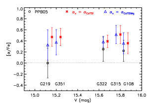
Figure 28.— Comparison of [$\alpha$/Fe] from high resolution ILS with line index estimates by Puzia et al. (2005) (PPB05, open circles) plotted as a function of V magnitude. Red crosses correspond to mean [$\alpha$/Fe] measured from Ca I, Ti I, Ti II and Si I only. Crosses are plotted with a $+0.05$ offset in V for visibility. Blue triangles correspond to mean [$\alpha$/Fe] from Ca I, Ti I, Ti II, Si I and Mg I.

Recent progress has been made in developing SSP IL spectra models with variable element ratios for comparison with Lick index absorption features (Thomas et al., 2003; Lee & Worthey, 2005; Schiavon, 2007). In particular, the models of Thomas et al. (2003) have made the [$\alpha$/Fe] estimates of a portion of M31 GCs possible, including three of those studied here (Puzia et al., 2005). In this case, [$\alpha$/Fe] is determined from a comparison with models of Lick indexes with Fe$-$dominated and Mg$-$dominated absorption features. A significant result of the study of (Puzia et al., 2005) is that GCs in M31 with ages $>$8 Gyrs have a mean [$\alpha$/Fe]$=+0.18\pm 0.05$ with a dispersion of 0.37 dex, which is $0.1\sim 0.2$ dex lower than what Puzia et al. (2005) find for Milky Way GCs. However, Beasley et al. (2005) find that the discrepancy between [$\alpha$/Fe] in M31 and Milky Way GCs may be an SSP model$-$dependent result.

Since we have found that [Mg/Fe] is likely to be depleted compared to other $\alpha-$elements within GCs due to AGB star self$-$pollution, we expect that [$\alpha$/Fe] ratios in GCs determined from indexes with Mg$-$dominated absorption features could be lower than the [$\alpha$/Fe] abundances that we determine from Ca, Si, or Ti.

To test this, we use the mean [$\alpha$/Fe] from Ca, Si and Ti lines for each GC (discussed in § 5.2) and compare to the [$\alpha$/Fe] estimated by Puzia et al. (2005) from Lick indexes in Figure 28. Measurements by Puzia et al. (2005) are plotted as open circles, and our mean [$\alpha$/Fe] excluding Mg are plotted as red crosses. We measure a systematically higher value for [$\alpha$/Fe] than Puzia et al. (2005) obtain for [$\alpha$/Fe] in all three GCs. The largest discrepancy is for G219, for which we find [$\alpha_{\rm{CaSiTi}}$/Fe]$=+0.47$ and Puzia et al. (2005) estimate [$\alpha$/Fe]$=0.0$. We find the discrepancy for G219 is reduced, but not resolved, if we include our [Mg/Fe]$=+0.04$ measurement in the mean [$\alpha$/Fe], which is shown by the blue triangle in Figure 28.

We note that, in addition to the degeneracy in the Lick indexes at low abundances, the effect of different [$\alpha$/Fe] ratios in SSP modeling at low abundances is also very weak, further obscuring the resolution of the Lick index measurements at low abundances, as already discussed by Maraston et al. (2003) and Puzia et al. (2005). It is likely that this is the cause of the remaining discrepancy in the [$\alpha$/Fe] estimate from low resolution for G219.

While our present sample size of high resolution IL abundances in extragalactic GCs is still small, it already removes some of the discrepancies between M31 and Milky Way GCs from Lick indexes that have been discussed in the literature (Puzia et al., 2005; Beasley et al., 2005; Brodie & Strader, 2006). We find that for this sample of GCs the true [$\alpha$/Fe] from Ca, Si, and Ti appear similar for the two galaxies, and that an accurate estimate of this value in GCs for interpretation of the chemical enrichment history of a galaxy must come from elements other than Mg due to the peculiarities of Mg abundances in GCs. Our results indicate that the unexpected, low [$\alpha$/Fe] ratios in metal-poor GCs may be an artifact of the uncertainties in line index systems at low metallicities.

6.4. Horizontal Branch Morphology

In general, the position of a star on the HB is a function of metallicity; it is expected that metal-poor GCs will have bluer HB morphologies than GCs with higher abundances. The fact that a number of Milky Way GCs at the same metallicity are observed to have very different HB morphologies has led to the conclusion that at least one important “second$-$parameter” plays a role in HB morphology (see review by Gallart et al., 2005). SSP models that reproduce the HBR$-$[Fe/H] relationship of the Milky Way are difficult to establish because HB morphology is sensitive to a variety of factors (e.g. mass loss, age, helium abundance, and others) (e.g. Lee et al., 1994; Recio-Blanco et al., 2006). Universal SSP models will be even more difficult to establish if the HBR$-$[Fe/H] relationship is different in other galaxies. There is evidence that this might indeed be the case; observations of GCs in both M31 and Fornax suggest the HBR$-$[Fe/H] relationship is offset to lower metallicities than in Milky Way GCs (Rich et al., 2005; Smith et al., 1998).

Low resolution studies have found it important to consider the effect of HB morphology on IL spectra of unresolved GCs because the presence of old, hot stars on the blue HB can mimic light from young main sequence stars, resulting in young or intermediate age determinations for GCs that are actually old (e.g. de Freitas Pacheco & Barbuy, 1995; Beasley et al., 2002; Schiavon et al., 2004). In the next section we discuss the effect of HB morphology on abundance and age determinations with our high resolution IL method.

6.4.1 Effect on Age and [Fe/H] Determinations

We have used our training set Milky Way GCs to perform tests to assess the effect of inaccurate proportions of red and blue HB stars on our results. The Teramo group has produced isochrones with two different values for mass loss during stellar post-main sequence evolution, a parameter which influences HB morphology. Of the two possible values, we have used isochrones with the less extreme mass loss parameter. This mass loss parameter produces very blue ($B-V\lesssim$ 0.1) HB stars for our 13 and 15 Gyr CMDs at [Fe/H] $\lesssim-1.8$, but does not produce bimodal HBs, as is common in many intermediate metallicity GCs. Because we are using the less extreme mass loss parameter, the fear is that the HB may not be as blue as appropriate in some cases.

Figure 29.— M31 GC spectra near H$\delta$ region, shown in order of increasing HBR from top to bottom.

To test the effect of this potential error, we have added blue HB stars by hand into our synthetic CMDs to ascertain the consequences of underpredicting the number of blue HB stars with our choice of isochrones. In these tests we conserve the total number of stars and total flux of the HB. We find that even though blue HB stars can contribute $10-15\%$ of the total flux of the population at wavelengths below 5000 Å, most of the Fe I lines are found over the range 4500-7000 Å, which is not as strongly influenced by the blue HB stars. Empirically, the addition of these stars into the CMD changes the derived Fe I abundances by $<+$0.05 dex. This is not unexpected, because MB08 showed that the Fe I EW strengths are dominated ($\sim 80\%$) by the luminous, cooler stars on the RGB, AGB and red HB, with little effect from hot turn off or hot blue straggler stars, particularly at redder wavelengths.

As an example of an extreme test case, we replaced all of the red HB stars with the same number of blue HB stars in the 10 Gyr best-fitting CMD for G219. We know from the HST CMDs of Rich et al. (2005) that G219 has both red HB stars and a large number of blue HB stars that are not entirely represented in the best-fitting CMD. Using this extreme CMD, we find that the Fe I abundance changes by $<$0.05 dex, the scatter in the Fe abundances increases, and the correlations of Fe abundance with EP, wavelength, and reduced EW get larger. From this extreme example, it is clear that not only do blue HB stars have little impact on the Fe I solution, but that accurate modeling of the red HB results in a much more self-consistent solution from all of the Fe I lines. Therefore, we can expect that having roughly the correct number of red HB stars in the synthetic CMDs will be more important for our abundance determinations than the correct number of blue HB stars. Given the small effect of blue HB stars on Fe I abundances, and given that our analysis only constrains the CMD age for old GCs to a 5 Gyr age range, we find that the accuracy of the blue HB morphology has a no significant (or even detectable) impact on our results. We conclude that the ages and metallicities that we derive for old GCs with our abundance analysis method will not be significantly affected by synthetic CMDs that have inaccurate blue HB morphologies.

As a further consistency check, we can look for qualitative information about the temperature distribution of the preferred CMD solutions in the Fe abundance vs. EP plots discussed in § 4.3. A symptom of too few hot, blue HB stars in the isochrone compared to the real GC would be increasing Fe abundances for lines with larger EP. For G108, G315, and G322 we find no significant trend in Fe abundance with EP, which implies that the distribution of stellar temperatures in the CMD solutions for these GCs are very accurate.

For G219 we find decreasing Fe abundances with increasing EP, which suggests in this case that we actually do have too many hot stars in the isochrone for this metal-poor GC. However, we also find higher Fe abundances at larger reduced EWs, which implies that we may have too many dwarf (low microturbulent velocity) stars in the isochrone being used in the analysis. Since the dwarf stars have higher temperatures than the giant stars, for G219 the excess of hot dwarf stars may cause the observed trends. Note that the dependence of Fe abundance on reduced EW may be associated with a small error in the microturbulence for some stars, as discussed in § 5.1. However, the mean Fe solution is not strongly affected by these weak trends, and so we do not pursue this issue further.

The only GC in the sample that shows the symptom of not enough hot stars in the Fe abundance vs. EP plot is G351, although it also shows the largest positive dependence of Fe abundance on reduced EW. The diagnostics suggest that there are both too many dwarf stars and not enough hot stars in the best CMD for G351. Also, the standard deviation for [Fe/H] is larger than for the other four GCs. While the solution for this cluster shows somewhat less self-consistency than for the other 4 clusters from the diagnostics discussed above, we emphasize that the overall scatter in the solution is still quite small, suggesting that our solution has not been dramatically affected by unavoidable problems (e.g. interloping stars or internal age or abundance variations) and that the statistical uncertainty is a meaningful estimate of the overall accuracy of the analysis. Moreover, any difficulties are not likely to be due to the HB morphology.

6.4.2 Consistency with Photometry

We are fortunate that the details of GC HB morphology do not have a large effect on the abundances or ages derived from high resolution IL spectra using this method. However, we can see the effect of HB stars on the temperature sensitive Balmer lines. We are still testing a method to constrain the HB morphology of unresolved GCs using the Balmer lines in high resolution IL spectra (J. Colucci et al. 2009, in preparation). For the purposes of this work, we simply check for qualitative consistency of the Balmer line profiles in the IL spectra with the HST CMDs of Rich et al. (2005). HBR ratios from Rich et al. (2005) for G108, G322, G351, and G219 are listed in Table 1, where a value of zero would correspond to a GC with a strongly red HB, and a value of unity would correspond to a GC with a strongly blue HB. From the IL spectra in the region of H$\delta$, shown in Figure 29, it is clear that G219 and G351 have more prominent Balmer line wings, and thus a larger contribution of flux from hot stars than G108, consistent with expectations.

Rich et al. (2005) measure an HBR$-$[Fe/H] relation from HST CMDs for 18 M31 GCs that is offset to lower metallicities than the HBR$-$[Fe/H] relation in Milky Way GCs. One explanation proposed is that the most metal-poor M31 GCs are $\sim 1-2$ Gyr younger than similar GCs in the Milky Way. We note that our lower preferred CMD age range for G219 is consistent with this, although we are unable to put strong constraints on absolute age.

6.5. Reddening Constraints from Broadband $B-V$ Colors

Table 12$E(B-V)$ Comparisons

	$E(B-V)$
Cluster	ILS Limit	1	2
G108-B045	0.13	0.18	0.10
G219-B358	0.06	0.06	0.06
G315-B381	0.08	0.17	$\cdots$
G322-B386	0.15	0.21	0.13
G351-B405	0.06	0.14	0.08

References. — (1.) Fan et al. (2008) (2.) Rich et al. (2005)

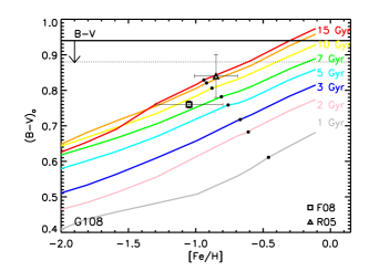
Figure 30.— Integrated $(B-V)_{0}$ colors calculated from synthetic CMDs are shown as a function of [Fe/H] for each age. Black points show the [Fe/H] and age solutions determined from this analysis for G108. The horizontal solid line corresponds to the observed $B-V$ color for the GC from Galleti et al. (2004), with an arrow and dotted line to show the $E(B-V)$ correction due to Galactic reddening of Schlegel et al. (1998). $(B-V)_{0}$ calculated with reddening and metallicity of Fan et al. (2008) (F08) and Rich et al. (2005) (R05) are plotted as open squares and triangles, respectively.

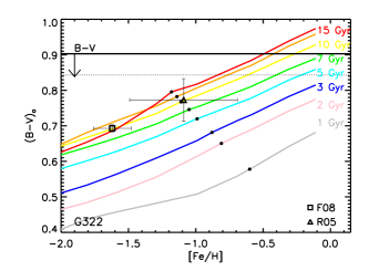
Figure 31.— Same as Figure 30 for G322.

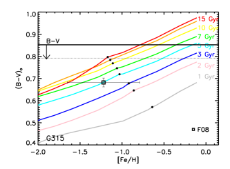
Figure 32.— Same as Figure 30 for G315.

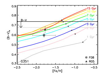
Figure 33.— Same as Figure 30 for G351.

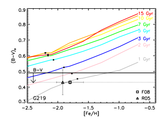
Figure 34.— Same as Figure 30 for G219.

In principle, an interesting additional constraint on our potential CMD solutions can be derived by comparing total broadband $(B-V)_{0}$ colors with existing photometry. This comparison could help us eliminate potential CMD solutions where the integrated colors of the CMDs are inconsistent with the photometry (see MB08). In practice, however, we find that reddening estimates for GCs in M31 are too uncertain to provide constraints on CMDs of the GCs discussed here. Rather, our abundance analysis constrains the CMD with enough fidelity that we can actually put some limits on the reddening for these individual M31 GCs. We note that GCs have previously been used in this way to probe reddening in galaxies (e.g. Barmby et al., 2000).

The colors for our synthetic CMDs using Teramo isochrones are shown in Figures 30 through 34. The broadband $(B-V)_{0}$ colors calculated from our synthetic CMDs are plotted against the [Fe/H] adopted in the Teramo isochrones for each GC. The trend of $(B-V)_{0}$ with [Fe/H] for constant age is emphasized by the solid colored lines. Black points correspond to the CMD and [Fe/H] solutions for each age described in § 4.3 for each GC. The black solid line in each figure corresponds to the observed $B-V$ color for the GC from the Revised Bologna Catalog (Galleti et al., 2004). Black arrows show the minimum reddening for the M31 line-of-sight of $E(B-V)=0.06$, which is due to Galactic extinction alone (Schlegel et al., 1998).

For each individual GC we show the recent reddening determination by Fan et al. (2008), who have derived these from correlations between optical and infrared colors and metallicity using a large set of M31 GC low resolution spectroscopic abundances. The $(B-V)_{0}$ calculated with the reddenings of Fan et al. (2008) are plotted as open squares, using the low resolution spectroscopic [Fe/H] solutions for the x-axis location. For G108, G322, G351 and G219 we also show the reddening adopted by the deep HST study of Rich et al. (2005), which is an average of several previous measurements. Reddenings of Rich et al. (2005) are plotted as open triangles at the [Fe/H] determined from their HST CMDs.

For each GC we can place an upper limit on the reddening that is consistent with the preferred CMDs for each GC discussed in § 5.1. This limit is calculated using the $(B-V)_{0}$ color of the youngest CMD in the preferred age range and the $B-V$ color from Galleti et al. (2004). The limits are listed in Table  6.5 with the values of Fan et al. (2008) and Rich et al. (2005) for comparison. We note that synthetic CMDs created with the Teramo isochrones that employ a higher mass loss rate than those used here, and thus have bluer HBs overall, would result in slightly lower predicted $(B-V)_{0}$. For the ages relevant here, the effect HB morphology is at most $\Delta(B-V)_{0}\sim-0.03$, and an indication of the uncertainty in our reddening limit.

In general, we find that our preferred CMDs and the reddenings they imply agree best with the [Fe/H] and reddenings of Rich et al. (2005), rather than with the reddenings inferred from low resolution spectroscopic metallicities. For G108, G322 and G351 the $E(B-V)$ derived by Fan et al. (2008) are higher than those adopted by Rich et al. (2005), but it is clear from Figures 30 through 34 that they are still consistent with an old ($>$10 Gyr) population at the metallicities applied by Fan et al. (2008).

Although G219 has been verified to be $\sim$10 Gyr or older by HST photometry, by low resolution spectral line indexes, and by high resolution spectra abundances in this work, it has $B-V$ colors substantially too blue for this age. This inconsistency has been noted in the Bologna catalog. In Table 6.5 we list the Galactic $E(B-V)=0.06$ as the only reliable constraint. We also note that the difference between the observed and predicted $B-V$ for G219 is too large to be explained by a deficit of blue HB stars in the synthetic CMD alone, but may be reduced with some contribution from relatively rare, but luminous, post-AGB or UV-bright stars (see Moehler, 2001).

For G351, the $B-V$ of the 10 Gyr CMD is consistent with $E(B-V)=0.0$, lower than the Galactic $E(B-V)=0.06$, which we again list as the most reliable constraint in Table 6.5. This difference in color may be at least partially explained by missing blue HB stars in the synthetic CMD as compared to the observed HST CMD in Rich et al. (2005).

G315 is the only GC discussed here for which there are no HST constraints available. We find an $E(B-V)\leq 0.08$ is consistent with our analysis. The larger value determined by Fan et al. (2008) is hard to understand because their derived reddening implies a $(B-V)_{0}$ that is inconsistent with an old population, even though the high and low resolution [Fe/H] are very similar. It is possible that the discrepancy can arise from inaccurate photometry used by Fan et al. (2008) to determine the $E(B-V)$.

7. Summary

We have applied a new method for detailed abundance analysis of high SNR, high resolution IL spectra of unresolved GCs to a sample of five GCs in M31. From over 60-100 resolved spectral lines in each cluster we have derived abundances from EWs for Mg, Al, Si, Ca, Sc, Ti, V, Cr, Mn, Fe, Co, Ni, Y and Ba. We have used our abundance analysis to put independent constraints on the ages and reddening of these M31 GCs, and used the high resolution IL spectra to measure velocity dispersions to high precision.

We find these 5 M31 GCs to be similar to the Milky Way GCs system in several respects. First, they are $>$10 Gyrs old, and span a range in [Fe/H] of $-2.2$ to $-0.9$. Second, their Ca, Si, and Ti abundances are enhanced to similar levels as Milky Way GCs, and suggesting that the gas reservoirs from which they formed were dominated by products of SNII at the time of their formation. Finally, the Fe$-$peak and the neutron capture abundance ratios studied here also follow Milky Way abundance trends.

We have confirmed that light element abundance variations between stars within GCs can effect abundances derived from high resolution IL spectra for Mg and possibly Al. We suggest that part of the large scatter in [$\alpha$/Fe] measurements of extragalactic GCs using low resolution line indexes may be due to the effects of Mg$-$dominated absorption features on line indexes.

We have demonstrated that a significant number of quantitative constraints on galaxy and GC formation and evolution can be made for unresolved GCs using this new abundance analysis technique. We have shown for the first time that abundance ratios fundamental to understanding galaxy formation can be obtained for other nearby, massive galaxies. While we have intentionally targeted “typical” GCs for this first sample in M31, a larger selection of GCs is crucial for a complete picture of the GC system and formation history of M31. Future work is needed to investigate other possible differences in the M31 GC system compared to the Milky Way, i.e. young GCs, high metallicity disk GCs, and enhanced nitrogen abundances.

Table 13Line Parameters and Integrated Light Equivalent Widths for M31 GCs

Species	$\lambda$	E.P.	log gf	EW(mÅ)	EW(mÅ)	EW(mÅ)	EW(mÅ)	EW(mÅ)
	(Å)	(eV)		G108	G322	G315	G351	G219
Mg I	4571.102	0.000	-5.691	$\cdots$	120.0	$\cdots$	86.7	34.5
Mg I	4703.003	4.346	-0.666	$\cdots$	139.2	$\cdots$	99.8	$\cdots$
Mg I	5528.418	4.346	-0.341	$\cdots$	$\cdots$	$\cdots$	147.3	58.2
Mg I	5528.418	4.346	-0.341	$\cdots$	$\cdots$	$\cdots$	143.6	$\cdots$
Al I	3944.016	0.000	-0.638	$\cdots$	$\cdots$	$\cdots$	$\cdots$	134.9
Al I	3944.016	0.000	-0.638	$\cdots$	$\cdots$	$\cdots$	$\cdots$	140.1
Si I	7405.790	5.610	-0.660	58.4	$\cdots$	$\cdots$	$\cdots$	$\cdots$
Si I	7415.958	5.610	-0.730	66.4	$\cdots$	50.1	$\cdots$	$\cdots$
Si I	7423.509	5.620	-0.580	84.3	66.5	82.4	$\cdots$	$\cdots$
Ca I	4318.659	1.899	-0.295	$\cdots$	109.6	$\cdots$	$\cdots$	$\cdots$
Ca I	4425.444	1.879	-0.358	127.9	$\cdots$	$\cdots$	$\cdots$	46.6
Ca I	5581.979	2.523	-0.555	99.0	77.6	86.3	64.2	$\cdots$
Ca I	5588.764	2.526	0.358	$\cdots$	138.0	137.6	122.8	59.8
Ca I	5590.126	2.521	-0.571	101.4	96.6	89.6	74.2	$\cdots$
Ca I	5601.286	2.526	-0.690	112.3	91.9	89.7	53.3	21.3
Ca I	5857.459	2.933	0.240	$\cdots$	124.0	145.0	111.9	43.1
Ca I	6122.226	1.886	-0.320	$\cdots$	$\cdots$	$\cdots$	149.8	69.0
Ca I	6162.180	1.899	-0.090	$\cdots$	$\cdots$	$\cdots$	$\cdots$	89.0
Ca I	6166.440	2.520	-1.142	84.4	64.6	71.0	$\cdots$	$\cdots$
Ca I	6439.083	2.526	0.390	$\cdots$	$\cdots$	$\cdots$	147.8	57.9
Ca I	6471.662	2.526	-0.686	98.9	$\cdots$	78.8	70.0	$\cdots$
Ca I	6493.781	2.521	-0.109	$\cdots$	$\cdots$	124.8	94.3	42.7
Ca I	6572.795	0.000	-4.310	82.5	$\cdots$	$\cdots$	$\cdots$	$\cdots$
Ca I	7148.150	2.709	0.137	$\cdots$	133.5	146.4	131.3	$\cdots$
Sc II	4246.837	0.315	0.240	$\cdots$	$\cdots$	141.7	$\cdots$	78.3
Sc II	4670.413	1.357	-0.580	84.3	86.4	86.9	$\cdots$	$\cdots$
Sc II	5526.821	1.768	0.020	79.4	62.2	76.5	52.2	$\cdots$
Sc II	6604.600	1.357	-1.480	44.6	$\cdots$	$\cdots$	$\cdots$	$\cdots$
Ti I	4991.072	0.836	0.380	$\cdots$	$\cdots$	$\cdots$	134.2	$\cdots$
Ti I	4999.510	0.826	0.250	143.5	122.0	134.8	129.7	$\cdots$
Ti I	5039.964	0.021	-1.130	115.9	$\cdots$	$\cdots$	$\cdots$	$\cdots$
Ti I	5210.392	0.048	-0.884	$\cdots$	140.1	$\cdots$	$\cdots$	$\cdots$
Ti I	5401.379	0.818	-2.890	$\cdots$	$\cdots$	9.4	$\cdots$	$\cdots$
Ti I	5648.565	2.495	-0.260	17.3	$\cdots$	$\cdots$	$\cdots$	$\cdots$
Ti I	5866.451	1.067	-0.840	88.4	71.7	$\cdots$	46.3	$\cdots$
Ti I	6743.127	0.900	-1.630	53.4	$\cdots$	55.3	30.5	$\cdots$
Ti II	4395.040	1.084	-0.660	$\cdots$	$\cdots$	$\cdots$	$\cdots$	106.5
Ti II	4395.848	1.243	-2.170	98.7	$\cdots$	$\cdots$	$\cdots$	$\cdots$
Ti II	4399.778	1.237	-1.270	137.7	$\cdots$	136.6	$\cdots$	$\cdots$
Ti II	4418.342	1.237	-2.460	85.2	$\cdots$	73.6	$\cdots$	$\cdots$
Ti II	4501.278	1.116	-0.760	$\cdots$	150.1	$\cdots$	$\cdots$	$\cdots$
Ti II	4563.766	1.221	-0.960	$\cdots$	155.6	136.4	126.3	68.9
Ti II	4571.982	1.572	-0.530	$\cdots$	$\cdots$	$\cdots$	156.5	76.7
Ti II	4589.953	1.237	-1.790	82.6	91.7	77.2	$\cdots$	44.5
Ti II	5381.010	1.566	-2.080	92.0	60.6	75.3	$\cdots$	$\cdots$
V I	6039.730	1.060	-0.650	39.5	$\cdots$	$\cdots$	$\cdots$	$\cdots$
V I	6081.430	1.050	-0.580	50.6	41.8	32.2	$\cdots$	$\cdots$
V I	6274.658	0.270	-1.670	37.6	$\cdots$	$\cdots$	$\cdots$	$\cdots$
Cr I	4254.346	0.000	-0.114	$\cdots$	$\cdots$	$\cdots$	$\cdots$	83.5
Cr I	4274.806	0.000	-0.231	$\cdots$	$\cdots$	$\cdots$	$\cdots$	67.3
Cr I	4274.806	0.000	-0.231	$\cdots$	$\cdots$	$\cdots$	$\cdots$	67.1
Cr I	5206.044	0.941	0.019	$\cdots$	$\cdots$	$\cdots$	$\cdots$	84.5
Cr I	5208.432	0.941	0.158	$\cdots$	$\cdots$	$\cdots$	$\cdots$	87.2
Cr I	5208.432	0.941	0.158	$\cdots$	$\cdots$	$\cdots$	$\cdots$	93.3
Cr I	5409.799	1.030	-0.720	$\cdots$	144.7	134.0	118.7	36.8
Cr I	7400.188	2.900	-0.111	85.9	$\cdots$	76.9	$\cdots$	$\cdots$
Mn I	4754.039	2.282	-0.086	103.9	73.1	80.4	$\cdots$	$\cdots$
Mn I	6013.520	3.070	-0.250	63.7	38.1	38.7	$\cdots$	$\cdots$
Mn I	6016.620	3.070	-0.216	73.4	$\cdots$	44.7	$\cdots$	$\cdots$
Mn I	6021.820	3.070	0.034	65.1	44.5	62.5	36.6	$\cdots$
Fe I	3878.027	0.958	-0.896	$\cdots$	$\cdots$	$\cdots$	$\cdots$	85.3
Fe I	3899.719	0.087	-1.515	$\cdots$	$\cdots$	$\cdots$	$\cdots$	143.7
Fe I	4063.605	1.557	0.062	$\cdots$	$\cdots$	$\cdots$	$\cdots$	133.0
Fe I	4071.749	1.608	-0.008	$\cdots$	$\cdots$	$\cdots$	$\cdots$	120.5
Fe I	4114.451	2.831	-1.303	72.4	$\cdots$	50.7	$\cdots$	$\cdots$
Fe I	4132.067	1.608	-0.675	$\cdots$	$\cdots$	$\cdots$	$\cdots$	93.4
Fe I	4132.908	2.845	-1.005	$\cdots$	$\cdots$	$\cdots$	$\cdots$	45.3
Fe I	4147.675	1.485	-2.071	$\cdots$	109.8	$\cdots$	$\cdots$	$\cdots$
Fe I	4154.505	2.831	-0.688	$\cdots$	$\cdots$	$\cdots$	$\cdots$	33.6
Fe I	4156.806	2.831	-0.808	$\cdots$	$\cdots$	131.7	$\cdots$	$\cdots$
Fe I	4157.788	3.417	-0.403	82.9	$\cdots$	71.8	$\cdots$	$\cdots$
Fe I	4174.917	0.915	-2.938	$\cdots$	100.8	75.8	$\cdots$	45.1
Fe I	4174.917	0.915	-2.938	$\cdots$	$\cdots$	113.5	$\cdots$	$\cdots$
Fe I	4175.643	2.845	-0.827	105.6	102.9	90.2	$\cdots$	20.0
Fe I	4181.764	2.831	-0.371	$\cdots$	$\cdots$	$\cdots$	$\cdots$	50.3
Fe I	4182.387	3.017	-1.180	82.1	$\cdots$	74.0	$\cdots$	$\cdots$
Fe I	4187.047	2.449	-0.514	$\cdots$	136.1	$\cdots$	$\cdots$	56.1
Fe I	4191.437	2.469	-0.666	$\cdots$	$\cdots$	$\cdots$	$\cdots$	59.5
Fe I	4195.340	3.332	-0.492	$\cdots$	$\cdots$	$\cdots$	123.5	$\cdots$
Fe I	4199.105	3.047	0.156	$\cdots$	$\cdots$	135.9	$\cdots$	$\cdots$
Fe I	4202.040	1.485	-0.689	$\cdots$	$\cdots$	$\cdots$	$\cdots$	96.3
Fe I	4206.702	0.052	-3.960	140.1	$\cdots$	115.6	87.1	$\cdots$
Fe I	4216.191	0.000	-3.357	$\cdots$	$\cdots$	$\cdots$	93.3	47.6
Fe I	4222.221	2.449	-0.914	120.7	110.4	119.6	$\cdots$	50.2
Fe I	4227.440	3.332	0.266	$\cdots$	$\cdots$	$\cdots$	$\cdots$	73.7
Fe I	4233.612	2.482	-0.579	$\cdots$	$\cdots$	142.9	$\cdots$	$\cdots$
Fe I	4250.130	2.469	-0.380	$\cdots$	$\cdots$	$\cdots$	$\cdots$	69.4
Fe I	4250.797	1.557	-0.713	$\cdots$	$\cdots$	$\cdots$	$\cdots$	86.4
Fe I	4260.486	2.399	0.077	$\cdots$	$\cdots$	$\cdots$	$\cdots$	94.9
Fe I	4271.164	2.449	-0.337	$\cdots$	$\cdots$	$\cdots$	$\cdots$	78.3
Fe I	4271.774	1.485	-0.173	$\cdots$	$\cdots$	$\cdots$	$\cdots$	138.1
Fe I	4282.412	2.176	-0.779	$\cdots$	$\cdots$	$\cdots$	131.8	86.8
Fe I	4325.775	1.608	0.006	$\cdots$	$\cdots$	$\cdots$	$\cdots$	139.1
Fe I	4337.055	1.557	-1.704	$\cdots$	127.5	$\cdots$	$\cdots$	$\cdots$
Fe I	4369.779	3.047	-0.803	$\cdots$	88.9	$\cdots$	$\cdots$	$\cdots$
Fe I	4404.761	1.557	-0.147	$\cdots$	$\cdots$	$\cdots$	$\cdots$	142.2
Fe I	4415.135	1.608	-0.621	$\cdots$	$\cdots$	$\cdots$	$\cdots$	121.6
Fe I	4427.317	0.052	-2.924	$\cdots$	$\cdots$	$\cdots$	$\cdots$	96.0
Fe I	4430.622	2.223	-1.728	$\cdots$	$\cdots$	138.1	$\cdots$	$\cdots$
Fe I	4442.349	2.198	-1.228	$\cdots$	135.2	144.2	$\cdots$	$\cdots$
Fe I	4443.201	3.071	-1.043	$\cdots$	$\cdots$	$\cdots$	$\cdots$	21.7
Fe I	4447.728	2.223	-1.339	$\cdots$	114.4	119.3	$\cdots$	$\cdots$
Fe I	4466.562	0.110	-0.600	$\cdots$	128.0	139.1	$\cdots$	$\cdots$
Fe I	4494.573	2.198	-1.143	$\cdots$	141.3	$\cdots$	$\cdots$	$\cdots$
Fe I	4602.949	1.485	-2.208	142.7	105.5	113.7	97.8	45.4
Fe I	4632.918	1.608	-2.901	107.6	$\cdots$	98.3	$\cdots$	$\cdots$
Fe I	4691.420	2.990	-1.523	$\cdots$	146.1	76.1	78.6	$\cdots$
Fe I	4736.783	3.211	-0.752	106.3	107.2	113.8	$\cdots$	$\cdots$
Fe I	4871.325	2.865	-0.362	$\cdots$	157.9	$\cdots$	$\cdots$	$\cdots$
Fe I	4872.144	2.882	-0.567	$\cdots$	158.2	$\cdots$	128.7	$\cdots$
Fe I	4890.763	2.875	-0.394	$\cdots$	$\cdots$	$\cdots$	154.0	$\cdots$
Fe I	4891.502	2.851	-0.111	$\cdots$	$\cdots$	$\cdots$	141.9	$\cdots$
Fe I	4903.316	2.882	-0.926	$\cdots$	130.6	137.8	123.8	$\cdots$
Fe I	4918.998	2.865	-0.342	$\cdots$	$\cdots$	$\cdots$	141.7	60.9
Fe I	4920.514	2.832	0.068	$\cdots$	$\cdots$	$\cdots$	$\cdots$	90.6
Fe I	4966.095	3.332	-0.871	125.4	$\cdots$	113.8	84.8	78.8
Fe I	4994.138	0.915	-2.969	137.1	125.1	112.6	128.7	$\cdots$
Fe I	5001.870	3.881	0.050	102.5	$\cdots$	92.2	109.0	$\cdots$
Fe I	5014.951	3.943	-0.303	102.9	$\cdots$	81.2	$\cdots$	$\cdots$
Fe I	5049.827	2.279	-1.355	$\cdots$	157.2	134.8	111.7	$\cdots$
Fe I	5051.640	0.915	-2.764	$\cdots$	158.7	144.0	124.4	$\cdots$
Fe I	5068.771	2.940	-1.041	132.4	111.5	106.9	85.8	$\cdots$
Fe I	5074.753	4.220	-0.160	85.2	$\cdots$	87.1	$\cdots$	$\cdots$
Fe I	5083.345	0.958	-2.842	$\cdots$	131.4	122.3	109.3	$\cdots$
Fe I	5110.435	4.260	-3.758	$\cdots$	$\cdots$	$\cdots$	136.0	$\cdots$
Fe I	5123.730	1.011	-3.058	$\cdots$	$\cdots$	$\cdots$	148.4	$\cdots$
Fe I	5127.368	0.915	-3.249	$\cdots$	113.9	$\cdots$	$\cdots$	$\cdots$
Fe I	5216.283	1.608	-2.082	142.5	122.4	140.3	95.9	$\cdots$
Fe I	5225.534	0.110	-4.755	114.2	$\cdots$	$\cdots$	$\cdots$	$\cdots$
Fe I	5232.952	2.940	-0.057	$\cdots$	$\cdots$	$\cdots$	141.9	$\cdots$
Fe I	5269.550	0.859	-1.333	$\cdots$	$\cdots$	$\cdots$	$\cdots$	156.0
Fe I	5281.798	3.038	-0.833	142.6	$\cdots$	101.9	75.1	$\cdots$
Fe I	5283.629	3.241	-0.524	$\cdots$	148.2	$\cdots$	$\cdots$	$\cdots$
Fe I	5383.380	4.312	0.645	126.4	97.9	103.7	94.4	34.0
Fe I	5393.176	3.241	-0.715	117.1	103.3	91.0	74.3	$\cdots$
Fe I	5397.141	0.915	-1.982	$\cdots$	$\cdots$	$\cdots$	$\cdots$	99.8
Fe I	5405.785	0.990	-1.852	$\cdots$	$\cdots$	$\cdots$	$\cdots$	108.9
Fe I	5424.080	4.320	0.520	149.5	108.2	111.9	115.4	39.2
Fe I	5429.706	0.958	-1.881	$\cdots$	$\cdots$	$\cdots$	$\cdots$	122.5
Fe I	5434.534	1.011	-2.126	$\cdots$	$\cdots$	$\cdots$	$\cdots$	98.7
Fe I	5446.924	0.990	-3.109	$\cdots$	$\cdots$	$\cdots$	$\cdots$	103.7
Fe I	5497.526	1.011	-2.825	$\cdots$	143.7	$\cdots$	135.7	66.6
Fe I	5501.477	0.958	-3.046	147.7	134.1	122.2	97.5	$\cdots$
Fe I	5506.791	0.990	-2.789	$\cdots$	155.3	$\cdots$	136.0	65.6
Fe I	5569.631	3.417	-0.500	128.1	104.9	101.2	$\cdots$	30.3
Fe I	5572.851	3.396	-0.275	$\cdots$	141.8	141.9	$\cdots$	38.9
Fe I	5576.099	3.430	-0.900	103.6	85.3	81.3	$\cdots$	$\cdots$
Fe I	5586.771	4.260	-0.096	$\cdots$	$\cdots$	145.2	$\cdots$	57.5
Fe I	5763.002	4.209	-0.450	74.3	73.5	85.5	$\cdots$	$\cdots$
Fe I	6136.624	2.453	-1.410	$\cdots$	$\cdots$	$\cdots$	$\cdots$	67.0
Fe I	6137.702	2.588	-1.346	$\cdots$	150.5	$\cdots$	105.5	54.6
Fe I	6151.623	2.180	-3.330	51.6	$\cdots$	47.2	$\cdots$	$\cdots$
Fe I	6173.341	2.220	-2.863	71.7	61.7	60.9	54.6	$\cdots$
Fe I	6180.209	2.730	-2.628	$\cdots$	$\cdots$	50.3	26.0	$\cdots$
Fe I	6187.995	3.940	-1.673	40.7	$\cdots$	26.7	$\cdots$	$\cdots$
Fe I	6200.321	2.610	-2.386	73.8	54.5	62.1	$\cdots$	$\cdots$
Fe I	6219.287	2.200	-2.428	99.1	$\cdots$	81.9	69.4	$\cdots$
Fe I	6229.232	2.830	-2.821	40.9	$\cdots$	29.9	$\cdots$	$\cdots$
Fe I	6230.736	2.559	-1.276	$\cdots$	$\cdots$	$\cdots$	125.2	44.7
Fe I	6246.327	3.600	-0.796	101.0	$\cdots$	91.9	91.7	$\cdots$
Fe I	6252.565	2.404	-1.767	120.9	$\cdots$	104.3	107.5	44.5
Fe I	6254.253	2.280	-2.435	114.4	$\cdots$	105.7	82.6	$\cdots$
Fe I	6265.141	2.180	-2.532	96.8	$\cdots$	94.8	72.4	$\cdots$
Fe I	6270.231	2.860	-2.543	46.0	$\cdots$	43.7	22.1	$\cdots$
Fe I	6297.799	2.220	-2.669	101.4	$\cdots$	$\cdots$	$\cdots$	$\cdots$
Fe I	6335.337	2.200	-2.175	$\cdots$	$\cdots$	108.9	81.7	31.0
Fe I	6336.830	3.690	-0.667	$\cdots$	$\cdots$	89.9	69.1	$\cdots$
Fe I	6355.035	2.840	-2.328	$\cdots$	$\cdots$	75.2	51.8	$\cdots$
Fe I	6393.612	2.430	-1.505	$\cdots$	$\cdots$	129.3	134.7	47.3
Fe I	6411.658	3.650	-0.646	$\cdots$	$\cdots$	94.4	73.5	$\cdots$
Fe I	6421.360	2.280	-1.979	$\cdots$	$\cdots$	$\cdots$	83.1	$\cdots$
Fe I	6430.856	2.180	-1.954	$\cdots$	$\cdots$	117.6	86.3	$\cdots$
Fe I	6481.878	2.280	-2.985	74.3	$\cdots$	$\cdots$	$\cdots$	$\cdots$
Fe I	6494.994	2.400	-1.246	$\cdots$	$\cdots$	$\cdots$	151.1	73.8
Fe I	6498.945	0.960	-4.675	94.2	$\cdots$	$\cdots$	$\cdots$	$\cdots$
Fe I	6546.252	2.750	-1.536	128.4	$\cdots$	$\cdots$	$\cdots$	$\cdots$
Fe I	6569.224	4.730	-0.380	61.6	52.7	$\cdots$	$\cdots$	$\cdots$
Fe I	6593.874	2.430	-2.377	$\cdots$	85.1	74.7	64.5	$\cdots$
Fe I	6677.997	2.690	-1.395	$\cdots$	$\cdots$	123.1	$\cdots$	30.5
Fe I	6703.576	2.760	-3.059	42.3	$\cdots$	39.9	$\cdots$	$\cdots$
Fe I	6710.323	1.480	-4.807	44.3	$\cdots$	$\cdots$	$\cdots$	$\cdots$
Fe I	6750.164	2.420	-2.592	89.7	71.8	71.1	86.3	$\cdots$
Fe I	6806.856	2.730	-2.633	32.6	$\cdots$	$\cdots$	$\cdots$	$\cdots$
Fe I	6839.835	2.560	-3.378	28.8	$\cdots$	$\cdots$	$\cdots$	$\cdots$
Fe I	6841.341	4.610	-0.733	$\cdots$	$\cdots$	41.1	$\cdots$	$\cdots$
Fe I	7130.925	4.300	-0.708	86.9	$\cdots$	$\cdots$	$\cdots$	$\cdots$
Fe I	7411.162	4.280	-0.287	$\cdots$	83.7	72.6	$\cdots$	$\cdots$
Fe I	7445.758	4.260	0.053	104.9	92.2	98.8	$\cdots$	$\cdots$
Fe I	7461.527	2.560	-3.507	55.7	$\cdots$	45.3	$\cdots$	$\cdots$
Fe I	7491.652	4.280	-1.067	70.1	55.8	$\cdots$	$\cdots$	$\cdots$
Fe I	7531.153	4.370	-0.557	$\cdots$	$\cdots$	64.1	$\cdots$	$\cdots$
Fe II	4178.859	2.583	-2.489	$\cdots$	61.6	51.1	$\cdots$	$\cdots$
Fe II	4178.859	2.583	-2.489	$\cdots$	$\cdots$	78.5	$\cdots$	$\cdots$
Fe II	4233.169	2.583	-1.900	$\cdots$	$\cdots$	131.2	$\cdots$	$\cdots$
Fe II	4508.289	2.856	-2.318	93.1	73.2	65.4	$\cdots$	$\cdots$
Fe II	4515.343	2.844	-2.422	102.1	84.3	97.1	$\cdots$	$\cdots$
Fe II	4541.523	2.856	-3.030	$\cdots$	$\cdots$	60.3	$\cdots$	$\cdots$
Fe II	4583.839	2.807	-1.890	130.1	131.4	140.2	131.0	61.2
Fe II	4923.930	2.891	-1.307	135.5	118.8	125.8	121.8	74.7
Fe II	5018.450	2.891	-1.292	$\cdots$	147.0	$\cdots$	136.7	84.1
Fe II	5534.848	3.245	-2.790	59.6	$\cdots$	$\cdots$	$\cdots$	$\cdots$
Fe II	6456.391	3.903	-2.075	$\cdots$	$\cdots$	56.0	$\cdots$	$\cdots$
Co I	6770.970	1.880	-1.970	49.5	$\cdots$	$\cdots$	$\cdots$	$\cdots$
Co I	6814.961	1.956	-1.900	45.8	$\cdots$	$\cdots$	$\cdots$	$\cdots$
Co I	6872.440	2.010	-1.850	51.9	$\cdots$	$\cdots$	$\cdots$	$\cdots$
Ni I	6586.319	1.951	-2.810	56.2	$\cdots$	$\cdots$	$\cdots$	$\cdots$
Ni I	6643.638	1.676	-2.300	97.8	97.7	83.3	$\cdots$	$\cdots$
Ni I	6767.784	1.826	-2.170	91.4	79.3	67.5	$\cdots$	$\cdots$
Ni I	7122.206	3.542	0.040	98.6	$\cdots$	$\cdots$	$\cdots$	$\cdots$
Ni I	7393.609	3.606	-0.270	$\cdots$	$\cdots$	66.8	$\cdots$	$\cdots$
Ni I	7414.514	1.986	-2.570	101.8	$\cdots$	63.3	$\cdots$	$\cdots$
Ni I	7422.286	3.635	-0.140	$\cdots$	63.3	62.8	$\cdots$	$\cdots$
Ni I	7525.118	3.635	-0.520	$\cdots$	$\cdots$	37.1	$\cdots$	$\cdots$
Y II	4883.690	1.084	0.070	72.0	$\cdots$	73.5	$\cdots$	$\cdots$
Ba II	4554.036	0.000	0.163	$\cdots$	$\cdots$	$\cdots$	$\cdots$	85.0
Ba II	4934.095	0.000	-0.157	$\cdots$	$\cdots$	$\cdots$	$\cdots$	90.5
Ba II	5853.688	0.604	-1.010	$\cdots$	$\cdots$	87.8	86.5	$\cdots$
Ba II	6141.727	0.704	-0.076	$\cdots$	142.4	$\cdots$	112.9	67.5
Ba II	6496.908	0.604	-0.377	$\cdots$	$\cdots$	$\cdots$	141.8	59.4

Note. —   Lines listed twice correspond to those measured in adjacent orders with overlapping wavelength coverage.

References

- Andrievsky et al. (2008) Andrievsky, S. M., Spite, M., Korotin, S. A., Spite, F., Bonifacio, P., Cayrel, R., Hill, V., & François, P. 2008, A&A, 481, 481
- Asplund et al. (2005) Asplund, M., Grevesse, N., & Sauval, A. J. 2005, in Astronomical Society of the Pacific Conference Series, Vol. 336, Cosmic Abundances as Records of Stellar Evolution and Nucleosynthesis, ed. T. G. Barnes, III & F. N. Bash, 25–+
- Barmby et al. (2002) Barmby, P., Holland, S., & Huchra, J. P. 2002, AJ, 123, 1937
- Barmby et al. (2000) Barmby, P., Huchra, J. P., Brodie, J. P., Forbes, D. A., Schroder, L. L., & Grillmair, C. J. 2000, AJ, 119, 727
- Barmby et al. (2007) Barmby, P., McLaughlin, D. E., Harris, W. E., Harris, G. L. H., & Forbes, D. A. 2007, AJ, 133, 2764
- Baumgardt & Makino (2003) Baumgardt, H., & Makino, J. 2003, MNRAS, 340, 227
- Baumueller & Gehren (1997) Baumueller, D., & Gehren, T. 1997, A&A, 325, 1088
- Beasley et al. (2004) Beasley, M. A., Brodie, J. P., Strader, J., Forbes, D. A., Proctor, R. N., Barmby, P., & Huchra, J. P. 2004, AJ, 128, 1623
- Beasley et al. (2005) —. 2005, AJ, 129, 1412
- Beasley et al. (2002) Beasley, M. A., Hoyle, F., & Sharples, R. M. 2002, MNRAS, 336, 168
- Bensby et al. (2005) Bensby, T., Feltzing, S., Lundström, I., & Ilyin, I. 2005, A&A, 433, 185
- Bergemann (2008) Bergemann, M. 2008, Physica Scripta Volume T, 133, 014013
- Bernstein & McWilliam (2002) Bernstein, R. A., & McWilliam, A. 2002, in IAU Symposium, Vol. 207, Extragalactic Star Clusters, ed. D. Geisler, E. K. Grebel, & D. Minniti, 739–+
- Bernstein & McWilliam (2005) Bernstein, R. A., & McWilliam, A. 2005, in Resolved Stellar Populations, ed. D. Valls-Gabaud & M. Chavez, Astronomical Society of the Pacific Conference Series
- Brodie & Strader (2006) Brodie, J. P., & Strader, J. 2006, ARA&A, 44, 193
- Burstein et al. (1984) Burstein, D., Faber, S. M., Gaskell, C. M., & Krumm, N. 1984, ApJ, 287, 586
- Carretta (2006) Carretta, E. 2006, AJ, 131, 1766
- Carretta et al. (2004) Carretta, E., Gratton, R. G., Bragaglia, A., Bonifacio, P., & Pasquini, L. 2004, A&A, 416, 925
- Castelli & Kurucz (2004) Castelli, F., & Kurucz, R. L. 2004, ArXiv Astrophysics e-prints
- Cescutti et al. (2008) Cescutti, G., Matteucci, F., Lanfranchi, G. A., & McWilliam, A. 2008, A&A, 491, 401
- Cohen (1978) Cohen, J. G. 1978, ApJ, 223, 487
- Cohen (2004) —. 2004, AJ, 127, 1545
- Cohen et al. (1999) Cohen, J. G., Gratton, R. G., Behr, B. B., & Carretta, E. 1999, ApJ, 523, 739
- Cordier et al. (2007) Cordier, D., Pietrinferni, A., Cassisi, S., & Salaris, M. 2007, AJ, 133, 468
- de Freitas Pacheco & Barbuy (1995) de Freitas Pacheco, J. A., & Barbuy, B. 1995, A&A, 302, 718
- Denisenkov & Denisenkova (1990) Denisenkov, P. A., & Denisenkova, S. N. 1990, Soviet Astronomy Letters, 16, 275
- Denissenkov et al. (1998) Denissenkov, P. A., Da Costa, G. S., Norris, J. E., & Weiss, A. 1998, A&A, 333, 926
- Djorgovski et al. (1997) Djorgovski, S. G., Gal, R. R., McCarthy, J. K., Cohen, J. G., de Carvalho, R. R., Meylan, G., Bendinelli, O., & Parmeggiani, G. 1997, ApJ, 474, L19+
- Faber et al. (1985) Faber, S. M., Friel, E. D., Burstein, D., & Gaskell, C. M. 1985, ApJS, 57, 711
- Faber & Jackson (1976) Faber, S. M., & Jackson, R. E. 1976, ApJ, 204, 668
- Fan et al. (2008) Fan, Z., Ma, J., de Grijs, R., & Zhou, X. 2008, MNRAS, 385, 1973
- Fenner et al. (2004) Fenner, Y., Campbell, S., Karakas, A. I., Lattanzio, J. C., & Gibson, B. K. 2004, MNRAS, 353, 789
- Ferguson et al. (2005) Ferguson, J. W., Alexander, D. R., Allard, F., Barman, T., Bodnarik, J. G., Hauschildt, P. H., Heffner-Wong, A., & Tamanai, A. 2005, ApJ, 623, 585
- Fulbright et al. (2006) Fulbright, J. P., McWilliam, A., & Rich, R. M. 2006, ApJ, 636, 821
- Gallart et al. (2005) Gallart, C., Zoccali, M., & Aparicio, A. 2005, ARA&A, 43, 387
- Galleti et al. (2004) Galleti, S., Federici, L., Bellazzini, M., Fusi Pecci, F., & Macrina, S. 2004, A&A, 416, 917
- Gehren et al. (2006) Gehren, T., Shi, J. R., Zhang, H. W., Zhao, G., & Korn, A. J. 2006, A&A, 451, 1065
- Geisler et al. (2005) Geisler, D., Smith, V. V., Wallerstein, G., Gonzalez, G., & Charbonnel, C. 2005, AJ, 129, 1428
- Girardi et al. (2000) Girardi, L., Bressan, A., Bertelli, G., & Chiosi, C. 2000, A&AS, 141, 371
- Gratton et al. (2004) Gratton, R., Sneden, C., & Carretta, E. 2004, ARA&A, 42, 385
- Gratton (1989) Gratton, R. G. 1989, A&A, 208, 171
- Gratton et al. (2001) Gratton, R. G., et al. 2001, A&A, 369, 87
- Harris (1991) Harris, W. E. 1991, ARA&A, 29, 543
- Harris (1996) —. 1996, AJ, 112, 1487
- Holland (1998) Holland, S. 1998, AJ, 115, 1916
- Huchra et al. (1991) Huchra, J. P., Brodie, J. P., & Kent, S. M. 1991, ApJ, 370, 495
- Huxor et al. (2005) Huxor, A. P., Tanvir, N. R., Irwin, M. J., Ibata, R., Collett, J. L., Ferguson, A. M. N., Bridges, T., & Lewis, G. F. 2005, MNRAS, 360, 1007
- Ivans et al. (2001) Ivans, I. I., Kraft, R. P., Sneden, C., Smith, G. H., Rich, R. M., & Shetrone, M. 2001, AJ, 122, 1438
- Ivans et al. (1999) Ivans, I. I., Sneden, C., Kraft, R. P., Suntzeff, N. B., Smith, V. V., Langer, G. E., & Fulbright, J. P. 1999, AJ, 118, 1273
- Iwamoto et al. (1999) Iwamoto, K., Brachwitz, F., Nomoto, K., Kishimoto, N., Umeda, H., Hix, W. R., & Thielemann, F.-K. 1999, ApJS, 125, 439
- Johnson et al. (2006) Johnson, J. A., Ivans, I. I., & Stetson, P. B. 2006, ApJ, 640, 801
- Kraft & Ivans (2003) Kraft, R. P., & Ivans, I. I. 2003, PASP, 115, 143
- Kraft et al. (1995) Kraft, R. P., Sneden, C., Langer, G. E., Shetrone, M. D., & Bolte, M. 1995, AJ, 109, 2586
- Kroupa (2001) Kroupa, P. 2001, MNRAS, 322, 231
- Kroupa (2002) —. 2002, Science, 295, 82
- Lee & Worthey (2005) Lee, H.-c., & Worthey, G. 2005, ApJS, 160, 176
- Lee & Carney (2002) Lee, J.-W., & Carney, B. W. 2002, AJ, 124, 1511
- Lee et al. (2005) Lee, J.-W., Carney, B. W., & Habgood, M. J. 2005, AJ, 129, 251
- Lee et al. (1994) Lee, Y.-W., Demarque, P., & Zinn, R. 1994, ApJ, 423, 248
- Letarte et al. (2006) Letarte, B., Hill, V., Jablonka, P., Tolstoy, E., François, P., & Meylan, G. 2006, A&A, 453, 547
- Mackey et al. (2006) Mackey, A. D., et al. 2006, ApJ, 653, L105
- Mackey et al. (2007) —. 2007, ApJ, 655, L85
- Maraston et al. (2003) Maraston, C., Greggio, L., Renzini, A., Ortolani, S., Saglia, R. P., Puzia, T. H., & Kissler-Patig, M. 2003, A&A, 400, 823
- Martin et al. (2006) Martin, N. F., Ibata, R. A., Irwin, M. J., Chapman, S., Lewis, G. F., Ferguson, A. M. N., Tanvir, N., & McConnachie, A. W. 2006, MNRAS, 371, 1983
- McLaughlin & van der Marel (2005) McLaughlin, D. E., & van der Marel, R. P. 2005, ApJS, 161, 304
- McWilliam (1997) McWilliam, A. 1997, ARA&A, 35, 503
- McWilliam (1998) —. 1998, AJ, 115, 1640
- McWilliam & Bernstein (2008) McWilliam, A., & Bernstein, R. A. 2008, ApJ, 684, 326
- McWilliam et al. (1995a) McWilliam, A., Preston, G. W., Sneden, C., & Searle, L. 1995a, AJ, 109, 2757
- McWilliam et al. (1995b) McWilliam, A., Preston, G. W., Sneden, C., & Shectman, S. 1995b, AJ, 109, 2736
- McWilliam & Rich (1994) McWilliam, A., & Rich, R. M. 1994, ApJS, 91, 749
- McWilliam et al. (2003) McWilliam, A., Rich, R. M., & Smecker-Hane, T. A. 2003, ApJ, 592, L21
- Melendez & Barbuy (2009) Melendez, J., & Barbuy, B. 2009, ArXiv e-prints
- Moehler (2001) Moehler, S. 2001, PASP, 113, 1162
- Morrison et al. (2004) Morrison, H. L., Harding, P., Perrett, K., & Hurley-Keller, D. 2004, ApJ, 603, 87
- Percival et al. (2009) Percival, S. M., Salaris, M., Cassisi, S., & Pietrinferni, A. 2009, ApJ, 690, 427
- Perrett et al. (2002) Perrett, K. M., Bridges, T. J., Hanes, D. A., Irwin, M. J., Brodie, J. P., Carter, D., Huchra, J. P., & Watson, F. G. 2002, AJ, 123, 2490
- Peterson (1989) Peterson, R. 1989, in Dynamics of Dense Stellar Systems, ed. D. Merritt, 161–166
- Pietrinferni et al. (2004) Pietrinferni, A., Cassisi, S., Salaris, M., & Castelli, F. 2004, ApJ, 612, 168
- Pietrinferni et al. (2006) —. 2006, ApJ, 642, 797
- Pritzl et al. (2005) Pritzl, B. J., Venn, K. A., & Irwin, M. 2005, AJ, 130, 2140
- Pryor & Meylan (1993) Pryor, C., & Meylan, G. 1993, in Astronomical Society of the Pacific Conference Series, Vol. 50, Structure and Dynamics of Globular Clusters, ed. S. G. Djorgovski & G. Meylan, 357–+
- Puzia et al. (2005) Puzia, T. H., Perrett, K. M., & Bridges, T. J. 2005, A&A, 434, 909
- Puzia et al. (2002) Puzia, T. H., Saglia, R. P., Kissler-Patig, M., Maraston, C., Greggio, L., Renzini, A., & Ortolani, S. 2002, A&A, 395, 45
- Ramírez & Cohen (2002) Ramírez, S. V., & Cohen, J. G. 2002, AJ, 123, 3277
- Recio-Blanco et al. (2006) Recio-Blanco, A., Aparicio, A., Piotto, G., de Angeli, F., & Djorgovski, S. G. 2006, A&A, 452, 875
- Rich et al. (2005) Rich, R. M., Corsi, C. E., Cacciari, C., Federici, L., Fusi Pecci, F., Djorgovski, S. G., & Freedman, W. L. 2005, AJ, 129, 2670
- Schiavon (2007) Schiavon, R. P. 2007, ApJS, 171, 146
- Schiavon et al. (2004) Schiavon, R. P., Rose, J. A., Courteau, S., & MacArthur, L. A. 2004, ApJ, 608, L33
- Schlegel et al. (1998) Schlegel, D. J., Finkbeiner, D. P., & Davis, M. 1998, ApJ, 500, 525
- Schweizer & Seitzer (1998) Schweizer, F., & Seitzer, P. 1998, AJ, 116, 2206
- Shetrone et al. (2003) Shetrone, M., Venn, K. A., Tolstoy, E., Primas, F., Hill, V., & Kaufer, A. 2003, AJ, 125, 684
- Shetrone et al. (2001) Shetrone, M. D., Côté, P., & Sargent, W. L. W. 2001, ApJ, 548, 592
- Shetrone & Keane (2000) Shetrone, M. D., & Keane, M. J. 2000, AJ, 119, 840
- Smecker-Hane & Wyse (1992) Smecker-Hane, T. A., & Wyse, R. F. G. 1992, AJ, 103, 1621
- Smith et al. (1998) Smith, E. O., Rich, R. M., & Neill, J. D. 1998, AJ, 115, 2369
- Sneden (1973) Sneden, C. 1973, ApJ, 184, 839
- Sneden et al. (2004) Sneden, C., Kraft, R. P., Guhathakurta, P., Peterson, R. C., & Fulbright, J. P. 2004, AJ, 127, 2162
- Sneden et al. (1997) Sneden, C., Kraft, R. P., Shetrone, M. D., Smith, G. H., Langer, G. E., & Prosser, C. F. 1997, AJ, 114, 1964
- Spitzer (1987) Spitzer, L. 1987, Dynamical evolution of globular clusters (Princeton, NJ, Princeton University Press, 1987, 191 p)
- Strader et al. (2009) Strader, J., Smith, G., Larsen, S., Brodie, J., & Huchra, J. 2009, ArXiv e-prints
- Tautvaišienė et al. (2004) Tautvaišienė, G., Wallerstein, G., Geisler, D., Gonzalez, G., & Charbonnel, C. 2004, AJ, 127, 373
- Thomas et al. (2003) Thomas, D., Maraston, C., & Bender, R. 2003, MNRAS, 339, 897
- Tinsley (1979) Tinsley, B. M. 1979, ApJ, 229, 1046
- Tolstoy et al. (2009) Tolstoy, E., Hill, V., & Tosi, M. 2009, ArXiv e-prints
- Tonry & Davis (1979) Tonry, J., & Davis, M. 1979, AJ, 84, 1511
- Venn et al. (2004) Venn, K. A., Irwin, M., Shetrone, M. D., Tout, C. A., Hill, V., & Tolstoy, E. 2004, AJ, 128, 1177
- Ventura & D’Antona (2008) Ventura, P., & D’Antona, F. 2008, A&A, 479, 805
- Vogt et al. (1994) Vogt, S. S., et al. 1994, in Society of Photo-Optical Instrumentation Engineers (SPIE) Conference Series, Vol. 2198, Society of Photo-Optical Instrumentation Engineers (SPIE) Conference Series, ed. D. L. Crawford & E. R. Craine, 362–+
- Whitmore & Schweizer (1995) Whitmore, B. C., & Schweizer, F. 1995, AJ, 109, 960
- Woosley & Weaver (1995) Woosley, S. E., & Weaver, T. A. 1995, ApJS, 101, 181
- Zinn & West (1984) Zinn, R., & West, M. J. 1984, ApJS, 55, 45