Critical parameters for the one-dimensional systems with long-range correlated disorder

Abstract

We study the metal-insulator transition in a tight-binding one-dimensional (1D) model with long-range correlated disorder. In the case of diagonal disorder with site energy within $[-\frac{W}{2},\frac{W}{2}]$ and having a power-law spectral density $S(k)\propto k^{-\alpha}$, we investigate the competition between the disorder and correlation. Using the transfer-matrix method and finite-size scaling analysis, we find out that there is a finite range of extended eigenstates for $\alpha>2$, and the mobility edges are at $\pm E_{c}=\pm|2-W/2|$. Furthermore, we find the critical exponent $\nu$ of localization length ($\xi\sim|E-E_{c}|^{-\nu}$) to be $\nu=1+1.4e^{2-\alpha}$. Thus our results indicate that the disorder strength $W$ determines the mobility edges and the degree of correlation $\alpha$ determines the critical exponents.

I Introduction

Anderson’s localization theory points out that in a system with uncorrelated diagonal disorder, all one-electron states are spatially localized with an exponentially decaying envelope with a characteristic localization length $\xi$, when the disorder strength is larger than a critical value.1 From the scaling theory,2 it is also well-known that an infinitesimal disorder can cause localization of all states in one and two dimensional systems in the thermodynamic limit. In recent years, it was found that spatial correlation of disorder potential played an important role in the nature of long-range charge transport of low-dimensional systems. In the presence of short-range correlated disorder, there exists a set of discrete resonant energy levels of extended states.3 ; 4 ; 5 ; 6 ; 7 ; 8 ; 9 ; 10 ; 11 ; 12 For example, a single extended eigenstate was found in the random dimer model,4 ; 8 ; 12 which was verified by measuring microwave transmission on the semiconductor superlattices with intentional correlated disorder.13 These models with short-range correlated disorder do not possess a true disorder induced metal-insulator transition in the thermodynamic limit. More recently, a one-dimensional (1D) disordered model with long-range correlation considered by de Moura and Lyra has arisen a great interest, as it can result in a continue band of extended states under appropriate conditions.14 The transition from localization to delocalization occurred at the critical points was examined experimentally in a single-mode waveguide with inserted correlated scatters.15 More recent experiments in ultra-cold atoms/Bose-Einstein condensate push the research in this direction further. bec

In the disordered systems, the critical parameters, such as the critical disorder strength $W_{c}$, mobility edge $E_{c}$, critical exponents $\nu_{E}$, $\nu_{W}$ (defined by the dependence of localization length on $W$ or $E$ near the critical points $\xi\sim|W-W_{c}|^{\nu_{W}}$ or $\xi\sim|E-E_{c}|^{\nu_{E}}$) are of particular importance and interest, since they determine the nature of the localization-delocalization transitions and the universal properties of disordered systems. Even for three-dimensional (3D) Anderson model which has been studied for more than forty years, the accurate determination of the critical parameters is still under recent investigations,16 where the critical parameters for different lattices are calculated and it was found that $\nu_{E}$ is close to $\nu_{W}$. While for 3D systems with scale-free disorder, it was found that $\nu_{E}\neq\nu_{W}$ and the extended Harris criterion is obeyed. 16b

In spite of many studies3 ; 4 ; 5 ; 6 ; 7 ; 8 ; 9 ; 10 ; 11 ; 12 ; 13 ; 14 ; 15 ; 17 ; 18 ; 19 ; 20 on the 1D systems with correlated disorder, many of them are in a perturbative level and there are still several important questions to be answered, such as the positions of the mobility edges and the value of the critical exponent $\nu$. The determination of these critical parameters and the comparison with the results of 3D models mentioned above will definitely deepen our understanding on disordered systems, especially the dependence on dimensionality and correlation. Moreover, the correlated disordered system is a kind of system which is intermediate between ordered system and pure disordered system. The investigation of the universal properties of this type system and comparison with quasi-periodic system is of fundamental importance. In addition, the accurate values of these critical parameters (mobility edges) have important applications in charge transport in low dimensional (correlated) disordered systems, such DNA molecules,21 , Bose-Einstein condensate in 1-D optical lattices with speckle potential.bec . In the present paper, we calculate these critical parameters for the 1D systems with the correlated diagonal disorder. And we also resolve some inconsistencies in the literatures.14 One of the advantages of our study is that we are able to investigate localization-delocalization transition and obtain the accurate critical parameters in 1D system with large size and the boundary effects is negligible, unlike the 3D system where all the sizes in three dimensions can not be very large due to the computational limitation.

We first investigate the localization properties of the 1D tight-binding model with long-range correlated diagonal disorder (the hopping constant is set to be unity). The diagonal on-site energies $\{\epsilon_{i}\}$ are distributed in $[-W/2,W/2]$ with $W$ being the strength of disorder. The site energies have a power-law spectral density $S(k)\propto k^{-\alpha}$ with $\alpha>0$. The function $S(k)$ is the Fourier transform of the two-point correlation function $\langle\epsilon_{i}\epsilon_{j}\rangle$ and $k$ is related to the wavelength $\lambda$ of the undulations on the random parameter landscape by $k=1/\lambda$.14 We find that the critical disorder width $W_{c}=4-2|E|$ at fixed energy $E$ for $\alpha>2$. Moreover, we can determine the positions of the mobility edges $\pm E_{c}=\pm|2-\frac{W}{2}|$, which separate the extended and localized energy eigenstates. The effective energy band width $B$ of the extended states has the linear relationship $B=4-W$ for $\alpha>2$. Thus, a phase diagram in the $(E,W)$ space is obtained. We also discuss the $\alpha$-dependence of the critical exponent $\nu$ of the localization length of the eigenstates. Interestingly, we find that the disorder strength $W$ determines the mobility edges and the degree of correlation $\alpha$ determines the critical exponents. Our results also indicate that the nature of a correlated disordered system is somehow between that of the pure random (without any correlation) and pseudo-random (quasi-periodic) systems. Our approach is non-perturbative and our results are hard to be obtained by perturbative calculations.

The organization of the paper is as follows. In the next section, we introduce the 1D disordered systems with long-range correlation and the basic approach in our calculation. In section III, we present our results of the mobility edge and critical exponents. The paper is summarized in section IV.

II Model and the Basic approach

We consider a 1D tight-binding Hamiltonian with long-range correlated disorder

$$H=\sum_{n}\epsilon_{n}|n\rangle\langle n|+\sum_{n}t(|n\rangle\langle n+1|+|n+1\rangle\langle n|),$$ (1)

where $|n\rangle$ is the Wannier state localized at site $n$ with on-site energy $\epsilon_{n}$, and $t$ is the nearest-neighbor hopping amplitude. We set $t=1$ for simplicity. The on-site energies $\{\epsilon_{n}\}$ can be constructed by the Fourier filtering method23 ; 24 ; 25 as follows: (i) generate a random sequence $\{u_{n}\}$ with a Gaussian distribution; (ii) get its Fourier components $\{u_{k}\}$ using the fast-Fourier transformation method; (iii) establish a new sequence $\{\epsilon_{k}\}$ by the relation $\epsilon_{k}=k^{-\alpha/2}u_{k}$; (iv) construct the sequence $\{\epsilon_{n}\}$, which is the inverse Fourier transform of $\{\epsilon_{k}\}$; (v) adjust the scale of the sequence $\{\epsilon_{n}\}$ reaching to $[-W/2,W/2]$. It can be checked that the disordered on-site energy $\{\epsilon_{n}\}$ is long-range correlated with the power spectrum $S(k)\propto\sum_{m}\langle\epsilon_{n}\epsilon_{n+m}\rangle e^{imk}\propto k^{-\alpha}$.26 The exponent $\alpha$ characterizing the correlation reflects the roughness of the energy sequence. The larger the value of $\alpha$ is, the smoother the energy landscape is.

The Schrödinger equation for the wavefunction amplitudes $\psi_{n}$ is

$$\epsilon_{n}\psi_{n}+\psi_{n-1}+\psi_{n+1}=E\psi_{n}.$$ (2)

Here, $E$ is the eigenenergy. Our interest focuses on the critical behavior in the thermodynamical limit. A useful way to find the critical points is based on the finite size analysis of the normalized localization length $\Lambda=\xi/N$ :26 If $\Lambda$ increases as the system size $N\rightarrow\infty$, which implies that $\xi$ would exceed $N$ when $N$ is large enough, the electron stays on a extended state; Otherwise, the state is localized, because $\Lambda$ is a decreasing function of $N$ and smaller than unity in the thermodynamic limit. So the $N$ dependent of $\Lambda=\xi/N$ can give the information of the localization-delocalization transition. Thereby, we can use this quantity $\Lambda$ to determine the critical disorder strength at fixed energy and the critical energies at fixed disorder strength.

In the regime of weak disorder, it was found17 that the localization length $\xi$ for a state of energy $E=2\cos\mu$ (not near band center and band edge) is determined by the correlation function of the disorder potential

$$\xi^{-1}=\gamma_{0}\varphi(\mu),$$ (3)

where $\gamma_{0}=\frac{\epsilon_{0}^{2}}{8\sin^{2}(\mu)}$, $\varphi(\mu)=1+2\sum_{m=1}^{\infty}\cos(2\mu m)q_{m}$, $\langle\epsilon_{n}\epsilon_{n+m}\rangle=\epsilon_{0}^{2}q_{m}$, $\langle\epsilon_{n}^{2}\rangle=\epsilon_{0}^{2}$. For our disordered system with long range correlation with the spectral density $S(k)\propto k^{-\alpha}$, the localization length has the normalized form $\Lambda=\xi/N\sim N^{\alpha-2}$, for $1\leq\alpha\leq 2$; $\Lambda\sim 1/N$, for $\alpha<1$. Thus we see that in the weak disorder regime the states are localized for $\alpha$ $<2$ and $\alpha=2$ is a critical value for the appearance of extended states.

To determine the full phase diagram and study the critical parameters, we use the transfer matrix method. Using the two-component vector $\Phi_{n}\equiv(\psi_{n},\psi_{n-1})^{T}$, where the superscript $T$ denotes the transpose, Eq. (2) can be written in a recursive form

$$\left(\begin{array}[]{c}\psi_{n+1}\\ \psi_{n}\end{array}\right)=M_{n}\left(\begin{array}[]{c}\psi_{n}\\ \psi_{n-1}\end{array}\right)$$ (8)

with

$$M_{n}=\left(\begin{array}[]{cc}E-\epsilon_{n}&-1\\ 1&0\\ \end{array}\right).$$ (11)

We obtain the transfer-matrix equation $\Phi_{N+1}=T_{N}\Phi_{1}$, with $T_{N}=\prod_{i=1}^{N}M_{i}$. The localization length $\xi$ at energy $E$ is the inverse of the Lyapunov coefficient $(\gamma>0)$, which is the largest eigenvalue of the limiting matrix $\lim_{N\rightarrow\infty}\ln(T_{N}T_{N}^{{\dagger}})^{1/2N}$.27 The large numbers appeared in the calculations have been took care of by dividing a large number and multiplying it at the end of calculation. The reorthogonalization method reorth has also been used and the same critical parameters are obtained. All the values of $\gamma$ in this paper are based on a geometrical mean of $10^{4}$ disorder configurations.

III Results and discussions

III.1 Critical disorder strength and mobility edges

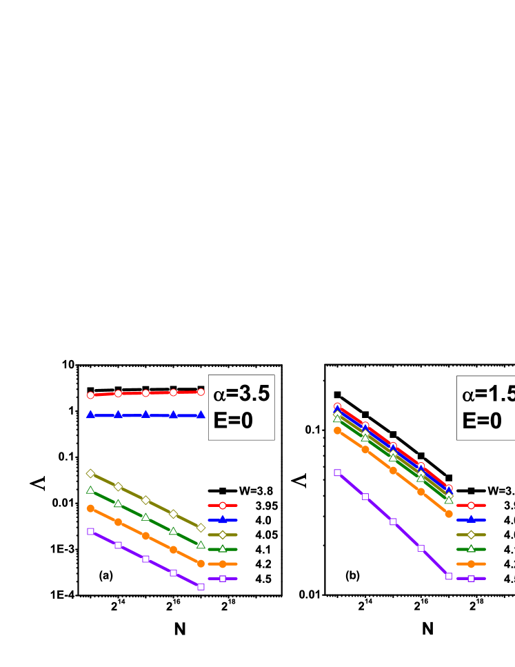
Figure 1: The normalized localization length $\Lambda\equiv\xi/N$ as a function of the system size $N$ for fixed $E=0$. $\alpha$ is taken as $3.5$ and $1.5$ in $(a)$ and $(b)$, respectively.

We perform the calculations of the normalized localization length $\Lambda$ for different values of $\alpha$ and energies. Figure 1 shows plots of the normalized localization length $\Lambda(W)$ versus $N$ for $E=0$, $\alpha=1.5$ and $\alpha=3.5$, respectively. The system size $N$ ranges from $2^{13}$ to $2^{17}$. We notice that $\Lambda$ is monotonically decreasing with $N$ for $\alpha=1.5$; while the picture is different for $\alpha=3.5$: the values of $\Lambda$ rise with increasing $N$ for $W<4$, whereas the values of $\Lambda$ decline with increasing $N$ for $W>4$. The size independence of $\Lambda$ at $W=4$ indicates a critical point of a continuous phase transition.

In Fig. 2, we display the dependence of $\Lambda$ on the disorder strength $W$ for the state of $E=1$ with typical values of $\alpha$. One may observe that there emerges an intersection point for different system size when $\alpha=2.5$, which corresponds to the critical point. This critical point doesn’t exist for $\alpha=1.5$. From the inset of Fig. 2, we could explicitly note the different dependence of $\Lambda$ on the system size $N$ in the vicinity of $W_{c}=2$. It tells us the state with $E=1$ is localized for $\alpha=1.5$ and is extended for $\alpha=2.5$ and $W<2$.

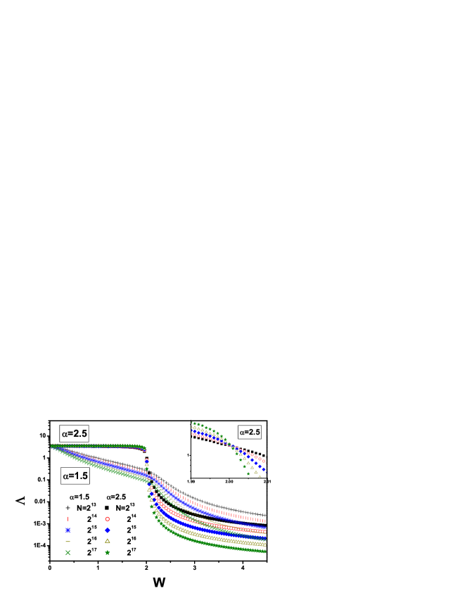
Figure 2: The normalized localization length $\Lambda$ as a function of the disorder width $W$ at fixed $E=1$ for systems with different size. $\alpha=1.5$ and $\alpha=2.5$. Insert: The detail behavior of $\Lambda(W)$ near the critical point $W_{c}=2$.

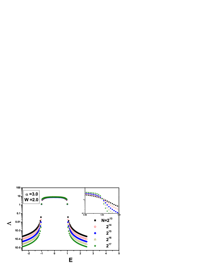
Figure 3: The normalized localization length $\Lambda$ as a function of $E$ at fixed $W=2$ for $\alpha=3.0$. Detail behavior of $\Lambda(E)$ near the critical point is shown in the inset.

Table I(a) lists the critical values of $W_{c}$ for various energies. It can be seen that the critical disorder strength is independent of $\alpha$ whenever $\alpha>2$. At the same time, we find a simple relationship between $W_{c}$ and $E$ as:

$$W_{c}=4-2|E|.$$ (12)

For the special state at band center with energy $(E=0)$, the critical value $W_{c}=4$, equals to the bandwidth. This conclusion for $E=0$ state was also reached by H. Shima et al.26

Using the same method, we also obtain the critical energies $\pm E_{c}$ at fixed $W$, as shown in Fig. 3. The results are given in Table I(b) for $\alpha>2$. The critical energies/the mobility edges can be determined by the following equations:

$$\pm E_{c}=\pm|2-\frac{W}{2}|~{}~{}~{}(\alpha>2).$$ (13)

The eigenstates between $-E_{c}$ and $E_{c}$ are delocalized. Therefore, the effective bandwidth $B$ of the delocalized states is (for $\alpha>2$)

$$B=|E_{c}-(-E_{c})|=4-W~{}~{}~{}(\alpha>2).$$ (14)

Figure 4 shows the phase diagrams in the $(W,E)$ and $(E,\alpha)$ plane. The critical value $\alpha=2$ is also consistent with the perturbative calculation discussed above. We emphasize that mobility edges or the effective bandwidth is only dependent on the disorder strength $W$ as long as $\alpha>2$. Also, in the limit of $W=0$, the effective bandwidth $B$ becomes $4$ which is the well-known result in the 1D ordered crystal lattice. It is interesting to compare with the pseudo random systems with quasi-periodic on-site energy $\varepsilon_{n}=\frac{W}{2}\cos(\pi Qn^{\alpha})\in[-\frac{W}{2},\frac{W}{2}]$, Q an irrational number, $0<\alpha<1$. In this model, the critical value $W_{c}=4-2|E|$ and the mobility is also at $\pm|2-W/2|$, independent of $\alpha$.28 The linear relations between the mobility edge $E_{c}$ (critical disorder strength $W_{c}$) and disorder strength $W$ (energy $E$) are simple and neat, further more they have a direct consequence on the critical exponents as will be discussed in the next subsection.

I(a) Critical values of disorder strength $W_{c}$ for different $\alpha$ and energies $E$

	E=-1.5	E=-1.0	E=-0.5	E=0.0	E=0.5	E=1.0	E=1.5
$\alpha$	$W_{c}$	$W_{c}$	$W_{c}$	$W_{c}$	$W_{c}$	$W_{c}$	$W_{c}$
2.50	1.000(1)	2.001(1)	3.001(2)	4.001(2)	3.001(2)	2.001(2)	1.000(2)
3.00	1.0000(4)	2.0000(5)	3.0001(5)	4.0001(6)	3.0001(6)	2.0001(6)	1.0001(4)
3.50	1.0000(1)	2.0000(1)	3.0000(1)	4.0000(1)	3.0000(1)	2.0000(1)	1.0000(1)
4.00	1.0000(1)	2.0000(1)	3.0000(1)	4.0000(1)	3.0000(1)	2.0000(1)	1.0000(1)

  I(b) Critical values of energies $\pm E_{c}$ for different $\alpha$ and disorder strength $W$

	W=3.0		W=2.0		W=1.0
$\alpha$	$-E_{c}$	$E_{c}$	$-E_{c}$	$E_{c}$	$-E_{c}$	$E_{c}$
2.50	-0.5004(6)	0.5003(5)	-1.0001(4)	1.0002(5)	-1.5001(5)	1.5001(5)
3.00	-0.5000(2)	0.5001(2)	-1.0000(3)	1.0000(2)	-1.5000(1)	1.5001(2)
3.50	-0.5000(1)	0.5000(1)	-1.0000(1)	1.0000(1)	-1.5000(1)	1.5000(1)
4.00	-0.5000(1)	0.5000(1)	-1.0000(1)	1.0000(1)	-1.5000(1)	1.5000(1)

Table 1: The values of critical disorder strength $W_{c}$ and critical energies (mobility edges) $\pm E_{c}$ obtained by the coordinates of the intersection points in the cases $\alpha>2$. The errors for the last digits are listed in the parentheses.

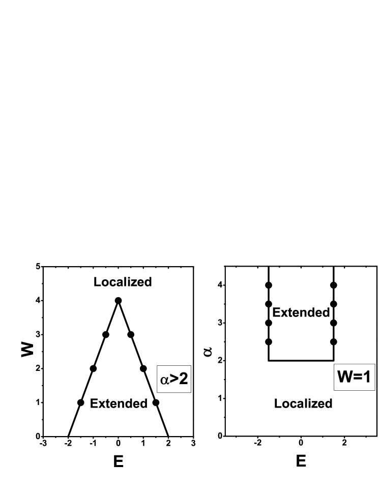
Figure 4: Phases diagrams in the $(W,E)$ and $(E,\alpha)$ plane. The delocalized and localized states are separated by $W=4-2|E|$ and $\alpha=2$. Here $t=1$. We take $W=1$ in $(E,\alpha)$ plane as an example.

III.2 Critical exponents based on finite-size Scaling Analysis

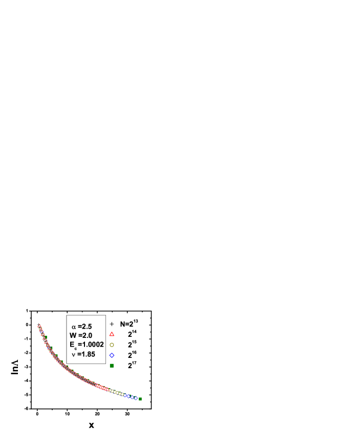
Figure 5: Scaling function of $\ln\Lambda$ for $\alpha=2.5$. Data from various chains, whose size $N$ ranges from $2^{13}$ to $2^{17}$, overlap each other. As an example, we give the optimized values of $E_{c}$ and $\nu$ in the case of $W=2.0$.

II(a) Critical values for disorder strength $W_{c}$ and exponent $\nu_{W}$ for different $\alpha$ and energy $E$

	E=0.0		E=0.5		E=1.0		E=1.5
$\alpha$	$W_{c}$	$\nu_{W}$	$W_{c}$	$\nu_{W}$	$W_{c}$	$\nu_{W}$	$W_{c}$	$\nu_{W}$
2.25	4.0015(5)	2.15(5)	3.0013(3)	2.13(4)	2.0008(7)	2.12(6)	1.0002(6)	2.12(6)
2.50	4.0007(5)	1.86(4)	3.0007(3)	1.83(3)	2.0004(3)	1.84(3)	1.0003(3)	1.81(3)
2.75	4.0003(3)	1.65(2)	3.0003(2)	1.65(2)	2.0001(2)	1.66(2)	1.0000(2)	1.66(3)
3.00	4.0002(1)	1.51(1)	3.0001(1)	1.50(1)	2.0001(1)	1.50(1)	1.0000(1)	1.50(2)
3.25	4.0000(1)	1.40(1)	3.0000(1)	1.40(1)	2.0000(1)	1.40(1)	1.0000(1)	1.41(2)
3.50	4.0000(1)	1.31(1)	3.0000(1)	1.30(1)	2.0000(1)	1.31(1)	1.0000(1)	1.31(1)
3.75	4.0000(1)	1.24(1)	3.0000(1)	1.24(1)	2.0000(1)	1.24(1)	1.0000(1)	1.25(2)
4.00	4.0000(1)	1.20(2)	3.0000(1)	1.19(1)	2.0000(1)	1.19(1)	1.0000(1)	1.20(2)
4.25	4.0000(1)	1.13(2)	3.0000(1)	1.13(1)	2.0000(1)	1.13(1)	1.0000(1)	1.14(1)
4.50	4.0000(1)	1.10(2)	3.0000(1)	1.10(1)	2.0000(1)	1.10(2)	1.0000(1)	1.11(2)

  II(b) Critical values for energy $E_{c}$ and exponent $\nu_{E}$ for different $\alpha$ and disorder strength $W$

	W=3.0		W=2.0		W=1.0
$\alpha$	$E_{c}$	$\nu_{E}$	$E_{c}$	$\nu_{E}$	$E_{c}$	$\nu_{E}$
2.25	0.5007(4)	2.15(4)	1.0004(3)	2.14(3)	1.5003(4)	2.12(4)
2.50	0.5003(2)	1.84(2)	1.0002(2)	1.85(2)	1.5001(2)	1.84(3)
2.75	0.5001(1)	1.66(1)	1.0001(1)	1.65(1)	1.5000(1)	1.66(1)
3.00	0.5001(1)	1.51(1)	1.0001(1)	1.51(1)	1.5000(1)	1.52(1)
3.25	0.5000(1)	1.40(1)	1.0000(1)	1.41(1)	1.4999(1)	1.43(2)
3.50	0.5000(1)	1.30(1)	1.0000(1)	1.31(1)	1.5000(1)	1.32(1)
3.75	0.5000(1)	1.24(1)	1.0000(1)	1.24(1)	1.5000(1)	1.25(1)
4.00	0.5000(1)	1.19(1)	1.0000(1)	1.19(1)	1.5000(1)	1.19(2)
4.25	0.5000(1)	1.14(1)	1.0000(1)	1.14(1)	1.5000(1)	1.15(1)
4.50	0.5000(1)	1.10(1)	1.0000(1)	1.10(2)	1.5000(1)	1.11(2)

Table 2: The values of critical exponent $\nu$ and critical points $W_{c}$ and $E_{c}$ got from the fitting $\Lambda$ with Eq. (10) for $\alpha>2$. The errors are obtained from bootstrap method with 95$\%$ confidence.

In the light of the finite-size scaling analysis, the normalized localization length $\Lambda$ for finite system may be related to the localization length $\xi_{\infty}$ for infinite system by the following scaling law:27

$$\ln\Lambda=f(\frac{N}{\xi_{\infty}}),$$ (15)

where the parameter $\xi_{\infty}$ varies as $\xi_{\infty}=|W-W_{c}|^{-\nu_{W}}$ or $\xi_{\infty}=|E\mp E_{c}|^{-\nu_{E}}$ in the vicinity of the critical point. Unlike three dimensional systems with usually small values of scaling variable (i.e. the size of cross section), in our one-dimensional systems, the irrelevant scaling exponents ander are of little effect due to scaling variable with very large values, i.e., the size of the system.

Firstly, we expand the scaling function in polynomial form:

$$\ln\Lambda=a_{0}+a_{1}x+a_{2}x^{2}+\cdot\cdot\cdot+a_{n}x^{n}.$$ (16)

Here $x$ defined as $x\equiv|W-W_{c}|N^{1/\nu_{W}}$ or $x\equiv|E\mp E_{c}|N^{1/\nu_{E}}$, is a nonlinear combination of $W(E)$ and $N$ with the parameters $W_{c}(\pm E_{c})$ and $\nu$ to be determined. Secondly, based on Eq. (10), we can obtain the values of $W_{c}(\pm E_{c})$ and $\nu$ by fitting $\Lambda$ which we got from previous calculation. The expansion in the scaling function must be carried up to $n$, that makes sure the degree of confidence reaches to $99\%$. As shown in Fig. 5, we have an excellent scaling curve, accompanied by the optimized values of $W_{c}(\pm E_{c})$ and $\nu$. The critical values for $W_{c}(\pm E_{c})$ obtained from finite-size scaling analysis are identical to those obtained in section III(A). The values of critical exponent $\nu$ and their errors estimated from the fitting procedure are given in Table II. It is clear that the critical exponent $\nu$ is independent on $W_{c}$ or $\pm E_{c}$. With increasing the correlation ($\alpha$), $\nu$ decreases to $1$. One may note that $\nu_{E}=\nu_{W}$. Actually it is a direct consequence of the linear relation between the disorder strength and mobility edges. From $\xi\sim|W-W_{c}|^{-\nu_{W}}$ and Eqs. (6) and (7), one finds that $\xi\sim|E-E_{c}|^{-\nu_{W}}$. Thus one has $\nu_{E}=\nu_{W}$. It is interesting to compare our results with those in 3D systems. For 3D Anderson model (without correlation) $\nu_{W}$ is close $\nu_{E}$, 16 while in the 3D system with scale free disorder, $\nu_{W}\neq\nu_{E}$. 16b

Then we find the dependence of $\nu$ on $\alpha$ follows the rule:

$$\nu=1+A_{1}\exp(A_{2}(2-\alpha)),$$ (17)

with $A_{1}$ is approximately $1.4$ and $A_{2}=1$ as seen in Fig. 6. We have found that $\nu=1$ for infinite large correlation of $\alpha$. It is interesting to note that the case with infinite large long-range correlation ($\alpha\rightarrow\infty$) looks like the quasiperiodic system, since the position of the mobility edges and the critical exponents (1) in both systems are the same. 28 In another limit situation $\alpha=2$, $\nu=2.4$, which is not easy to be obtained from direct calculation due to the critical slowing down phenomena. This result is apparently different from $\nu=2$ at $\alpha=2$ mentioned in Ref. 14 . Our results are based on finite size scaling. The data show very good scaling behavior as shown in Fig. 5. The critical exponents and mobility edges are obtained simultaneously by using fitting formula Eq. (10). The mobility edges obtained in this way are identical to those obtained in section III(A). Therefore our results are reliable. It is interesting that the mobility edges are determined only by the disorder strength $W$ and the critical exponents are determined only by the degree of correlation $\alpha$.

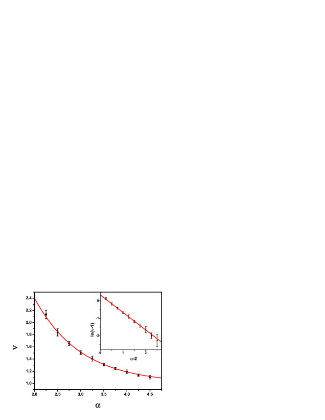
Figure 6: The $\alpha$-dependence of the averaged critical exponent $\nu$ (for different values of $W_{c}$ and $E_{c}$) and the fitting curve from Eq. (11) with $A_{1}=1.4$ and $A_{2}=1$. Inset: $\ln(\nu-1)$ as a function of $\alpha-2$, where the straight slope is set to $-1$.

IV Conclusion

In summary, we have investigated the universal localization properties of 1D tight-binding model where the disorder is long-range correlated with a power-law spectral density $S(k)\propto k^{-\alpha}$, $\alpha>0$. We have obtained the complete phase diagram and neat results for the critical parameters. There is a finite range of extended eigenstates, and the effective bandwidth decreases linearly with increasing $W$ for $\alpha>2$. The positions of the mobility edges separating localized and extended states depend only on the disorder strength whenever $\alpha>2$. Using the finite-size scaling analysis, we find the critical exponent $\nu=1+1.4\exp(2-\alpha)$. In particular $\nu=2.4$ when $\alpha=2$ and $\nu=1$ when $\alpha\rightarrow\infty$. Compared to the 3D uncorrelated Anderson model, the positions of the mobility edges are apparently different. And the critical exponent $\nu$ is no longer equal to $1.58$ 16 ; ander . So, the transition in the 1D disordered system with correlation is in a new universal class. The existence of mobility edge and $\alpha$ dependence of the critical exponent indicate that the nature of a correlated disordered system is somehow between that of the pure random (without any correlation) and pseudo-random (quasi-periodic) systems. Our work sheds some light on the metal-insulator transitions.

V Acknowledgements

This work is supported in part by the National Natural Science of China under No. 10574017, 10744004, 10874020, National Fundamental Research of China grant under No. 2006CB921400 and a grant of the China Academy of Engineering and Physics.

References

- (1) P. W. Anderson, Phys. Rev. 109, 1492 (1958).
- (2) E. Abrahams, P. W. Anderson, D. G. Licciardello, and T. V. Ramakrishnan, Phys. Rev. Lett. 42, 673 (1979).
- (3) J. C. Flores, J. Phys. Condens. Matter 1, 8471 (1989).
- (4) D. H. Dunlap, H. L. Wu, and P. Phillips, Phys. Rev. Lett. 65, 88 (1990).
- (5) H.-L. Wu and P. Phillips, Phys. Rev. Lett. 66, 1366 (1991).
- (6) S. N. Evangelou and D. E. Katsanos, Phys. Lett. A 164, 456 (1992).
- (7) A. Bovier, J. Phys. A 25, 1021(1992).
- (8) S. N. Evangelou and A. Z. Wang, Phys. Rev. B 47, 13126 (1993).
- (9) J. C. Flores and M. Hilke, J. Phys. A 26, L1255 (1993).
- (10) M. Hilke, J. Phys. A 27, 4773 (1994).
- (11) F. C. Lavarda, M. C. dos Santos, D. S. Galvão, and B. Laks, Phys. Rev. Lett. 73, 1267 (1994).
- (12) J. Heinrichs, Phys. Rev. B 51, 5699 (1995).
- (13) V. Bellani, E. Diez, R. Hey, L. Toni, L. Tarricone, G. B. Parravicini, F. Domínguez-Adame, and R. Gómez-Alcalá, Phys. Rev. Lett. 82, 2159 (1999).
- (14) F. A. B. F. de Moura and M. L. Lyra, Phys. Rev. Lett. 81, 3735 (1998).
- (15) U. Kuhl, F. M. Izrailev, A. A. Krokhin, and H.-J. Stöckmann, Appl. Phys. Lett. 77, 633 (2000).
- (16) G. Roati, C. D’Errico, L. Fallani, M. Fattori, C. Fort, M. Zaccanti, G. Modugno, M. Modugno and M. Inguscio Nature 453, 895 (2008); J. Billy, V. Josse, Z. Zuo, A. Bernard, B. Hambrecht, P. Lugan, D. Clement, L. Sanchez-Palencia, P. Bouyer and A. Aspect, Nature 453, 891 (2008).
- (17) A. Eilmes, A. M. Fischer, and R. A. Römer, Phys. Rev. B 77, 245117 (2008).
- (18) M. L. Ndawana, R. A. Römer, M. Schreiber, Europhys. Lett. 68, 678-684 (2004).
- (19) F. M. Izrailev and A. A. Krokhin, Phys. Rev. Lett. 82, 4062 (1999).
- (20) S. Russ, J. W. Kantelhardt, A. Bunde, and S. Havlin, Phys. Rev. B 64, 134209 (2001).
- (21) Wei Zhang and Sergio E. Ulloa, Phys. Rev. B 69, 153203 (2004).
- (22) Wei Zhang and Sergio E. Ulloa, Phys. Rev. B 74, 115304 (2006).
- (23) P. Carpena, P. Bernaola-Galan, P. C. Ivanov, and H. E. Stanley, Nature (London) 418, 955(2002); 421, 764 (2003); D. Holste, I. Grosse, and H. Herzel, Phys. Rev. E 64, 041917 (2001); Wei Zhang and Sergio E. Ulloa, Microelectronics Journal 35, 23 (2004).
- (24) D. Saupe, in The Science of Fractal Images, edited by H.-O. Peitgen and D. Saupe (Springer, New York, 1988); J. Feder, Fractals (Plenum Press, New York, 1988).
- (25) C.-K. Peng, S. Havlin, M. Schwartz, and H. E. Stanley, Phys. Rev. A 44, R2239 (1991).
- (26) S. Prakash, S. Havlin, M. Schwartz, and H. E. Stanley, Phys. Rev. A 46, R1724 (1992).
- (27) H. Shima, T. Nomura, and T. Nakayama, Phys. Rev. B 70, 075116 (2004).
- (28) B. Kramer and A. McKinnon, Rep. Prog. Phys. 56, 1469 (1993).
- (29) A. MacKinnon and B. Kramer, Z.Phys. B 53, 1 (1983).
- (30) S. Das Sarma, S. He, and X. C. Xie, Phys. Rev. Lett. 61, 2144 (1988); Phys. Rev. B 41, 5544 (1990).
- (31) K. Slevin and T. Ohtsuki, Phys. Rev. Lett. 82, 382 (1999).