Double humped states in the nonlinear Schrödinger equation with a random potential

Abstract

The role of double humped states in spreading of wave packets for the nonlinear Schrödinger equation (NLSE) with a random potential is explored and the spreading mechanism is unraveled. Comparison with an NLSE with a double-well potential is made. There are two independent affects of the nonlinearity on the double humped states for the NLSE: coupling to other states and destruction. The interplay between these effects is discussed.

We consider the discrete nonlinear Schrodinger equation with a random potential in one dimension:

$$i\frac{\partial\psi_{n}}{\partial t}=-\psi_{n+1}-\psi_{n-1}+\epsilon_{n}\psi_{n}+\beta\left|\psi_{n}\right|^{2}\psi_{n}$$ (1)

Where $\epsilon_{n}$ are random potentials chosen uniformly from the interval $\left[-2,2\right]$ and $\beta$ is a positive constant. For $\beta=0$ this is the Anderson model, where all the states are localized. Consequently, a wave packet that is initially localized will remain localized in the vicinity of its initial position. A question that is subject to extensive research is whether Anderson localization can survive the nonlinear term $\beta\left|\psi\right|^{2}\psi$ Shepelyansky (1993). Numerical simulations indicate that for (1) Anderson localization is destroyed and subdiffusion takes place Flach et al. (2009a); Pikovsky and Shepelyansky (2008); Molina (1998); Skokos et al. (2009); Flach et al. (2009b). Heuristic arguments were developed in order to explain these results Pikovsky and Shepelyansky (2008); Skokos et al. (2009); Shepelyansky (1993), but the detailed mechanism of possible spreading is not clear. Resonances between eigenstates of the linear model, namely (1) with $\beta=0$ provide a reasonable mechanism for spreading and it is the subject of the present paper.

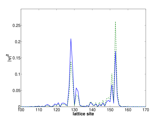
Double humped states $\varphi_{+},\varphi_{-}$ are two eigenstates of the Hamiltonian (1) which are localized over the same two sites that are far in real space while their energies are very close. An example for such states appears in Fig.1. According to Rabi’s formula, in the linear case ($\beta=0$), if one places (at time $t=0$) a wave packet on the site of one hump and the states are exactly symmetric or antisymmetric with respect to the interchange of the humps, one finds the packet on the other site in time $t$ with the probability

$$P_{12}\left(t\right)=\sin^{2}\left(\Delta E\frac{t}{2\hbar}\right)$$ (2)

where $\Delta E$ is the difference between the energies of the two double humped states and the time period is $T_{Rabi}=\frac{2\pi\hbar}{\Delta E}$. The period is preserved also for the case when the symmetry of the hump interchange is broken, as in the case of the random potential. This mechanism of jumping between sites has proved to be the main mechanism for low frequency ac conductivity in disordered media Sivan and Imry (1987). It is expected that its behavior may be strongly affected by the nonlinear term. For a double-well potential the low energy states are symmetric and antisymmetric double humped states, with the humps in the centers of the wells. In the absence of nonlinearity, (2) holds. But, for sufficiently strong nonlinearity the wavepacket will be confined to the initial well Soffer and Weinstein (2005); Sacchetti (2009). In the present work we would like to explore if double humped states contribute to a mechanism of resonant spreading in the NLSE.

Figure 1: A pair of double humped states for the linear system ($\beta=0$). The states are marked with blue solid line and green dashed line.

In our study, we would like to distinguish between resonant spreading (caused by the double humped states) and diffusive spreading from one state to its neighbors. For this purpose, we had to find realizations where the humped states are located far from each other (in comparison with the localization length, in our case $\xi\approx 6$). The probability to find double humped states with humps located at a distance $L$ is proportional to $\exp\left(-L/\xi\right)$ Sivan and Imry (1987) and therefore realizations which couple states located far from each other are very rare (as we are looking for them in a finite region in real space). In order to overcome this problem and create a pool of realizations with double humped states in some region in real space, we have developed a strategy for “double humps hunting”. We choose some random potential having localized eigenstates in the linear case (Anderson localization). We focus on two sites so that we will have double humped states which are localized on these two sites. These sites will be denoted by $O$ and $P$ in what follows. The Hamiltonian of this realization is diagonalized, which results in a diagonal matrix with eigenenergies on the diagonal. Now, we vary the site energy of the original model on one site (say $P$) of the two sites mentioned above. According to Feynman-Hellman theorem, when we increase monotonically the potential of a site, its energy is monotonically increasing and we can easily find a point where the two diagonal terms are approximately equal. Since we change the realization, the Hamiltonian is not diagonal anymore and the sites are coupled by matrix elements of the order of $\exp\left(-L/\xi\right)$. Taking the potential realization which creates almost identical energies in the diagonal of the Hamiltonian (written in the initial eigenstates basis), we can usually construct double humped states for this realization. In this way, we found a set of realizations having double humped states with distance of 25 sites (about 4 localization lengths in our case) between the humped sites.

After choosing appropriate realizations, we had to know which values of $\beta$ should be chosen in order to see the influence of the double humps. If we choose very small values of $\beta$, the system will behave similarly to the linear case and a wave packet initially localized on one humped site will oscillate between the humped sites for very long times. However, for large values of $\beta$, the linear eigenstates become irrelevant very quickly (compared to the period of the oscillations) and the correlation between the double humped states is broken before they have a chance to affect the dynamics. Moreover, high values of $\beta$ suppress the oscillations between the humped states even in the double-well case Sacchetti (2009) where there is no mixing with other states. So, we have to choose the $\beta$ values very carefully. For this purpose, we use a double-well model Tsukada (2001) to set the scale of the effect of $\beta$. In particular we find numerically for each disorder realization a value of $\beta_{\frac{1}{4}}$ for which only $\frac{1}{4}$ of the wave function oscillates between the humped sites $O$ and $P$ when the double humped states are detached in the computation from all other states. When we run the dynamics of (1) for double humped realizations with $\beta=\beta_{\frac{1}{4}}$, we can see clearly the influence of the resonance and we are still able to observe spreading for reasonable times.

In other words, the nonlinearity has two effects: destroying the double humped states and populating other states of the linear model. In order to distinguish the two effects we compare to the double-well model with a nonlinear term, where the two lowest energy states can be assumed isolated from the other states.

The difference between the double-well model and (1) is that in the double-well model only two states participate in the dynamics (see appendix) and only these were taken into account for this model. Therefore, numerical calculations for the double-well model are much faster and allow us to estimate the behavior of (1) without performing time consuming (split-step) calculations. In addition, the dynamics in the double-well problem is periodic and gives us the time scale of the oscillations. Deviations of (1) from the double-well model appear when additional states become involved in the dynamics. This happens, naturally, when we increase $\beta$. So, first we should calculate $\beta_{c}$, the largest $\beta$ for which the double-well model dynamics is still similar to (1) and make sure that $\beta_{c}>\beta_{\frac{1}{4}}$ (otherwise, our results for $\beta_{\frac{1}{4}}$ will have no clear meaning for the NLSE). We have located an initial wave packet $\overrightarrow{y_{O}}$ around one of the humps (as a superposition of the two double humped states) at site $O$. We have followed the population difference between the double humped states in the double-well model and in the NLSE during one time period $T$ which is numerically calculated for each realization based on the nonlinear double-well model (see appendix). $\beta_{c}$ was defined as the highest $\beta$ value for which $\frac{1}{T}\int_{0}^{T}\left(w_{double-well}-w_{NLSE}\right)^{2}dt<0.001$ where $w$ denotes the population difference. $\beta_{c}$ is expected to be high when the overlap between the double humped states and other states in the system is small and we can see a correlation between $\beta_{c}$ and the parameter

$$R^{-1}=\sum_{i}{}^{{}^{\prime}}\left|\frac{V_{i}^{OOO}}{E_{O}-E_{i}}\right|$$ (3)

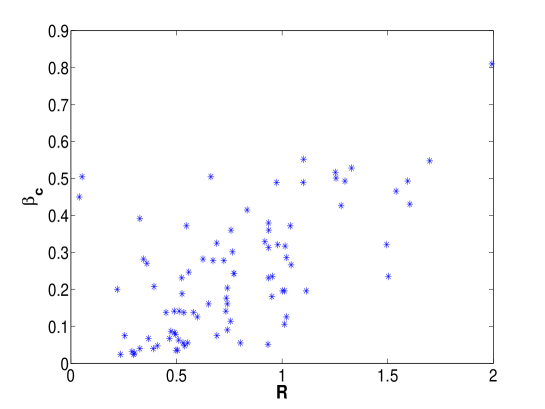
The index $i$ in the sum runs over all the eigenstates on the lattice except for the two double humped states. $E_{O}$ is the energy of the initial wave localized at site $O$ and $E_{i}$ are the eigenvalues of the system. The numerator is $V_{i}^{OOO}\equiv\sum_{n}y_{O,n}^{3}\cdot v_{i,n}$ where the eigenfunctions with center of localization at site $i$ are denoted by $\overrightarrow{v_{i}}$ and $v_{i,n}$ is the $n$ component of vector $\overrightarrow{v_{i}}$ while $y_{O,n}$ is the $n$ component of $\overrightarrow{y_{O}}$. The reasoning for the importance of (3) is explained in Flach et al. (2009a); Skokos et al. (2009); Flach et al. (2009b) (where $R$ is defined in a slightly different way) and the correlation to $\beta_{c}$ is shown in Fig. 2. The correlation deteriorates when $V_{i}^{OOO}$ is replaced by other quartic combinations of components of $\overrightarrow{y_{O}}$ and $\overrightarrow{v_{i}}$.

Figure 2: Correlation between $R$ and $\beta_{c}$ (blue asterisks).

In order to see the influence of the double humped states in specific realizations, we should compare them to realizations where such states are broken that will be named “broken realizations”. The “broken realizations” are the same set of realizations as the realizations where double humped states are found except for one fundamental difference - we have changed the disorder potential in one of the humped sites to be zero, namely $\epsilon_{P}=0$, and by this broke the coupling and destroyed the double humped states without causing qualitative changes to the other eigenstates of the system. For each pair of double humped and “broken” realizations, we have chosen an initial wavefunction $\overrightarrow{y_{O}}$ located around $O$ as a superposition of the two double humped states and followed the evolution of the wavefunction. The evolution of the wavepacket in time was calculated according to (1) with $\beta=\beta_{\frac{1}{4}}$ using the split step method Skokos et al. (2009). A quantity which interests us when we measure the spreading of a wavefunction is the second moment, defined as

$$m_{2}=\sum_{n}\left(n-\bar{n}\right)^{2}\left|\psi_{n}\right|^{2}$$ (4)

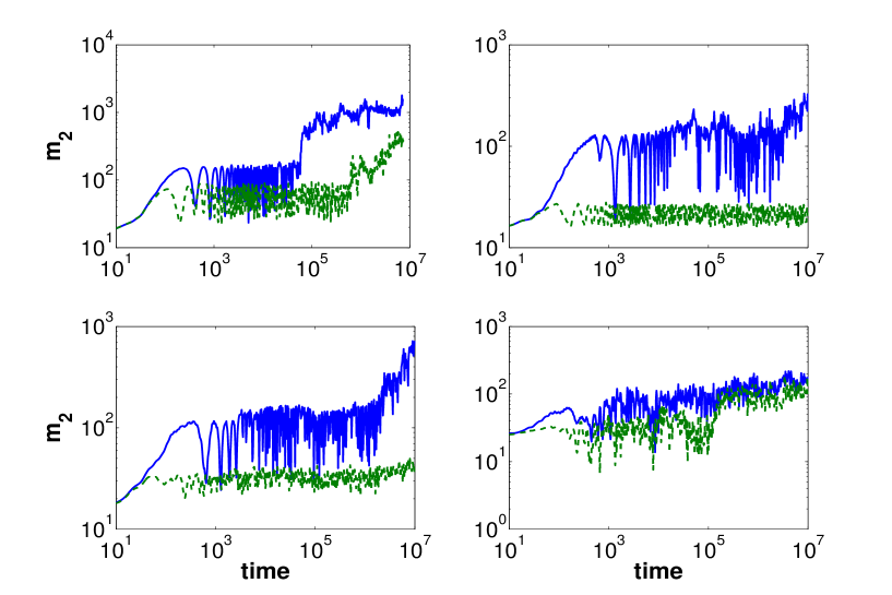
where $\overline{n}=\sum_{n}n\left|\psi_{n}\right|^{2}$ is the averaged location of the wavefunction. When we compare the growth in the second moment for double humped realizations and the broken realizations, we see that the second moment of the double humped realizations grows faster, when the realizations are selected as was outlined above and in both cases the initial wave packet is localized at $O$. Some examples are presented in Fig. 3. We examined 25 realizations of this form and the behavior presented in Fig. 3 is representative of all of them. This indicates that double humped states do substantially contribute to the spreading process of a wavefunction more than typical states.

In conclusion, we see that in the presence of nonlinearity that is not too strong, the spreading of a wave packet prepared initially near some site $O$ is substantially stronger if there is a double humped state with one of its humps near $O$, than if the states peaked near $O$ are single humped. We found that there is a regime of values where $\beta$ is sufficiently small so that the double humped structure is preserved but the packet is not only oscillating between the humps but also leaks to other states, leading to spreading. In order to find this nonlinearity regime, we have used the double-well model to isolate the two double humped states from the other eigenstates of (1) with $\beta=0$. We found that if $\beta$ is small enough so that the oscillations between the two states are not suppressed in the double-well model, then the double humped states will contribute to the spreading for the NLSE. Since double humped states are suppressed and do not contribute to the spreading for high nonlinearities, we can not conclude that they dominate the spreading of the NLSE. Exploring what is the dominant mechanism for this problem is left for future a research.

Figure 3: The second moment as function of time for a representative double humped (solid blue) and broken (dashed green) realizations for wave packets started in the vicinity of $O$.

Appendix- Double-well model

In order to predict the response of the double humped states to variations of $\beta$, we first investigate a model where only two states exist, the double-well model. In this way we avoid the influence of the other states of the NLSE. For this model, the NLSE is

$$i\frac{\partial\Psi\left(r,t\right)}{\partial t}=-\nabla^{2}\Psi\left(r,t\right)+\left[\epsilon\left(r\right)+\beta\left|\Psi\left(r,t\right)\right|^{2}\right]\Psi\left(r,t\right)$$ (5)

where $\epsilon\left(r\right)$ is the double-well potential. It is convenient to write the wavefunction in the form Raghavan et al. (1999)

$$\Psi\left(r,t\right)=\psi_{1}\left(t\right)\phi_{1}\left(r\right)+\psi_{2}\left(t\right)\phi_{2}\left(r\right)$$ (6)

where $\phi_{1}\left(r\right)$ and $\phi_{2}\left(r\right)$ are symmetric and antisymmetric combinations of the double humped eigenstates (and therefore they are orthogonal) while $\psi_{1}\left(t\right)$, $\psi_{2}\left(t\right)$ are the amplitudes of $\phi_{1}\left(r\right)$, $\phi_{2}\left(r\right)$ at time $t$. Eq. (5) takes the form:

$$i\left[\phi_{1}\frac{d\psi_{1}}{dt}+\phi_{2}\frac{d\psi_{2}}{dt}\right]=-\left[\psi_{1}\nabla^{2}\phi_{1}+\psi_{2}\nabla^{2}\phi_{2}\right]+\left[\epsilon\left(r\right)+\beta\left|\Psi\left(r,t\right)\right|^{2}\right]\Psi\left(r,t\right)$$ (7)

After multiplying both sides by $\phi_{1}\left(r\right)$ ($\phi_{1}$ and $\phi_{2}$ are localized and therefore they can be chosen to be real) and integrating over $r$, (7) becomes

$$i\frac{d\psi_{1}}{dt} = -\int\left[\psi_{1}\phi_{1}\nabla^{2}\phi_{1}+\psi_{2}\phi_{1}\nabla^{2}\phi_{2}\right]dr+\int\epsilon\left[\phi_{1}^{2}\psi_{1}+\phi_{2}\phi_{1}\psi_{2}\right]dr$$

$$+ \beta\int dr\left[\psi_{1}^{2}\psi_{1}^{*}\phi_{1}^{4}+\left(\psi_{1}^{2}\psi_{2}^{*}+2\left|\psi_{1}\right|^{2}\psi_{2}\right)\phi_{1}^{3}\phi_{2}+\right.$$

$$+ \left.\left(2\left|\psi_{2}\right|^{2}\psi_{1}+\psi_{2}^{2}\psi_{1}^{*}\right)\phi_{1}^{2}\phi_{2}^{2}+\left|\psi_{2}\right|^{2}\psi_{2}\phi_{2}^{3}\phi_{1}\right]$$

Following Tsukada (2001), it is convenient to write (Appendix- Double-well model) as

$$\frac{d\psi_{1}}{dt} = -i\left(\omega_{1}+\Omega_{1}\left|\psi_{1}\right|^{2}\right)\psi_{1}-iK\psi_{2}$$

$$-i\left(2A_{1}\psi_{2}+A_{1}\psi_{1}^{2}\psi_{2}^{*}+B\psi_{2}^{2}\psi_{1}^{*}+A_{2}\left|\psi_{2}\right|^{2}\psi_{2}-2A_{1}\left|\psi_{2}\right|^{2}\psi_{2}\right)$$

where

$$\omega_{1}=-\int\left(\left|\nabla\phi_{1}\right|^{2}+\epsilon\phi_{1}^{2}+2\beta\phi_{1}^{2}\phi_{2}^{2}\right)dr$$ (10)

$$\Omega_{1}=-\beta\int\left(\phi_{1}^{4}-2\phi_{1}^{2}\phi_{2}^{2}\right)dr$$

$$K=-\int\left(\nabla\phi_{1}\nabla\phi_{2}+\epsilon\phi_{1}\phi_{2}\right)$$

$$A_{1}=-\beta\int\phi_{1}^{3}\phi_{2}dr$$

$$A_{2}=-\beta\int\phi_{2}^{3}\phi_{1}dr$$

$$B=-\beta\int\phi_{1}^{2}\phi_{2}^{2}dr$$

and we have used the relation $\left|\psi_{1}\right|^{2}+\left|\psi_{2}\right|^{2}=1$. In a similar way,

$$\frac{d\psi_{2}}{dt} = -i\left(\omega_{2}+\Omega_{2}\left|\psi_{2}\right|^{2}\right)\psi_{2}-iK\psi_{1}$$

$$-i\left(2A_{2}\psi_{1}+A_{2}\psi_{2}^{2}\psi_{1}^{*}+B\psi_{1}^{2}\psi_{2}^{*}+A_{1}\left|\psi_{1}\right|^{2}\psi_{1}-2A_{2}\left|\psi_{1}\right|^{2}\psi_{1}\right)$$

where

$$\omega_{2}=-\int\left(\left|\nabla\phi_{2}\right|^{2}+\epsilon\phi_{2}^{2}+2\beta\phi_{1}^{2}\phi_{2}^{2}\right)dr$$ (12)

and

$$\Omega_{2}=-\beta\int\left(\phi_{2}^{4}-2\phi_{1}^{2}\phi_{2}^{2}\right)dr$$

In order to establish the connection with the double humped states of (1), the coefficients of (10) and (12) were taken from the the Schrödinger Eq. (1). First we have expressed these coefficients for the linear case $\beta=0$ where only $\omega_{1}$, $\omega_{2}$ and $K$ do not vanish. For this purpose we find $\varphi_{+}$ and $\varphi_{-}$, the double humped eigenstates of (1) for $\beta=0$. the amplitudes $\psi_{1}\left(t\right)$ and $\psi_{2}\left(t\right)$ of the symmetric and antisymmetric combinations

$$\phi_{1}\left(r\right)=\frac{1}{\sqrt{2}}\left(\varphi_{+}+\varphi_{-}\right)$$ (13)

$$\phi_{2}\left(r\right)=\frac{1}{\sqrt{2}}\left(\varphi_{+}-\varphi_{-}\right)$$ (14)

satisfy the Schrödinger Eqs. (Appendix- Double-well model) and (Appendix- Double-well model). Therefore, When we write the Hamiltonian (1) in a basis composed from $\phi_{1}$ and $\phi_{2}$ in addition to all the single humped eigenstates of (1), $K$ will appear as an off diagonal term which couples $\phi_{1}$ and $\phi_{2}$ while $\omega_{1}$ and $\omega_{2}$ will appear as diagonal terms. In the nonlinear case, $K$ stays the same while $\omega_{1,2}=\omega_{1,2}^{linear}-2\beta\int\phi_{1}^{2}\phi_{2}^{2}dr$. In order to find the corrections to $\omega_{1,2}$ for the nonlinear Hamiltonian and to calculate all the other coefficients (10) and (12), we find numerically the vectors $\phi_{1}$ and $\phi_{2}$ with the help of (13) and (14) from (1) as explained above.

It is convenient to follow the dynamics described by the variables $u=\psi_{1}\psi_{2}^{*}+\psi_{2}\psi_{1}^{*}$, $v=-i\left(\psi_{1}\psi_{2}^{*}-\psi_{2}\psi_{1}^{*}\right)$ and $w=\left|\psi_{1}\right|^{2}-\left|\psi_{2}\right|^{2}$. After some simple procedures, we obtain a vector equation of the motion Tsukada (2001),

$$\frac{d\overrightarrow{\rho}}{dt}=\overrightarrow{\rho}\times\overrightarrow{T}$$ (15)

in which $\overrightarrow{\rho}=\left(u,v,w\right)$ is a vector characterizing the state of the coupled system on the unit sphere, i.e., $u^{2}+v^{2}+w^{2}=1$, and, $\overrightarrow{T}=\left(T_{1},T_{2},T_{3}\right)$ where

$$T_{1}=\omega_{1}-\omega_{2}+\frac{1}{2}\Omega_{1}\left(1+w\right)-\frac{1}{2}\Omega_{2}\left(1-w\right)+\left(A_{1}-A_{2}\right)u$$ (16)

$$T_{2}=-Bv$$ (17)

$$T_{3}=2K+2\left(A_{1}+A_{2}\right)+Bu-A_{1}\left(1-w\right)-A_{2}\left(1+w\right)$$ (18)

It is easy to find (numerically) $w\left(t\right)$ which gives us the time period and the amplitude of the double-well oscillations. For small nonlinearities, these results are good estimations of the NLSE behavior on a lattice. In this work, we have used (15) to find $\beta_{\frac{1}{4}}$ values. For this purpose, we have chosen an initial value for $w$ which represents a wavepacket localized around site $O$. Following the dynamics of $w(t)$ for different values of nonlinearity $\beta$, we have found the maximal $\beta$ for which at least $\frac{1}{4}$ of the wavepacket is oscillating between sites $O$ and $P$. This $\beta$ is $\beta_{\frac{1}{4}}$.

References

- Shepelyansky (1993) D. L. Shepelyansky, Phys. Rev. Lett. 70, 1787 (1993), ISSN 0031-9007, and references therein.
- Flach et al. (2009a) S. Flach, D. O. Krimer, and C. Skokos, Phys. Rev. Lett. 102, 024101 (2009a), URL http://arxiv.org/abs/0805.4693v2.
- Pikovsky and Shepelyansky (2008) A. S. Pikovsky and D. L. Shepelyansky, Phys. Rev. Lett. 100, 094101 (2008), ISSN 0031-9007.
- Molina (1998) M. I. Molina, Phys. Rev. B 58, 12547 (1998), ISSN 1098-0121.
- Skokos et al. (2009) C. Skokos, D. O. Krimer, S. Komineas, and S. Flach, Phys. Rev. E 79 (2009), arXiv:0901.4418.
- Flach et al. (2009b) S. Flach, D. O. Krimer, and C. Skokos, Phys. Rev. Lett. 102, 209903 (2009b).
- Sivan and Imry (1987) U. Sivan and Y. Imry, Phys. Rev. B 35, 6074 (1987).
- Soffer and Weinstein (2005) A. Soffer and M. I. Weinstein, Phys. Rev. Lett 95, 213905 (2005).
- Sacchetti (2009) A. Sacchetti (2009).
- Tsukada (2001) N. Tsukada, phys. Rev. A 64, 033601 (2001).
- Raghavan et al. (1999) S. Raghavan, A. Smerzi, S. Fantoni, and S. Shenoy, Phys. Rev. A 59, 620 (1999).