Photometric Calibration of the Supernova Legacy Survey Fields 

Abstract

Aims. We present the photometric calibration of the Supernova Legacy Survey (SNLS) fields. The SNLS aims at measuring the distances to SNe Ia at ($0.3<z<1$) using MegaCam, the 1 deg² imager on the Canada-France-Hawaii Telescope (CFHT). The uncertainty affecting the photometric calibration of the survey dominates the systematic uncertainty of the key measurement of the survey, namely the dark energy equation of state. The photometric calibration of the SNLS requires obtaining a uniform response across the imager, calibrating the science field stars in each survey band (SDSS-like $ugriz$ bands) with respect to standards with known flux in the same bands, and binding the calibration to the $UBVRI$ Landolt standards used to calibrate the nearby SNe from the literature necessary to produce cosmological constraints.

Methods. The spatial non-uniformities of the imager photometric response are mapped using dithered observations of dense stellar fields. Photometric zero-points against Landolt standards are obtained. The linearity of the instrument is studied.

Results. We show that the imager filters and photometric response are not uniform and publish correction maps. We present models of the effective passbands of the instrument as a function of the position on the focal plane. We define a natural magnitude system for MegaCam. We show that the systematics affecting the magnitude-to-flux relations can be reduced if we use the spectrophotometric standard star BD +17 4708 instead of Vega as a fundamental flux standard. We publish $ugriz$ catalogs of tertiary standards for all the SNLS fields.

1 Introduction

As we enter an era of precision supernova cosmology, photometric calibration becomes an increasingly important contribution to the systematic error budgets. All cosmology oriented surveys have therefore undertaken ambitious calibration efforts in order to “break the 1% barrier”. A notable example is the work published by the Sloan Digital Sky Survey (SDSS) (Ivezić et al., 2007; Padmanabhan et al., 2008). Major future surveys are also planning ambitious photometric calibration programs, relying on stellar calibrator observations and in-situ laboratory measurements (Burke, 2007; Magnier, 2007; Keller et al., 2007; Stubbs & Tonry, 2006; Tucker et al., 2007).

An example of a program demanding a better than 1% photometric precision is the measurement of the cosmological parameters using Type Ia Supernovae (SNe Ia) (Astier et al., 2006; Wood-Vasey et al., 2007; Riess et al., 2007). This measurement is all about comparing the luminosity distances of a set of distant SNe Ia with those of their nearby counterparts. High-z ($z\sim 0.7$) SN Ia distances are determined from measurements taken with the redder bands of the survey ($r$, $i$ and $z$), a model of the SNe Ia spectral energy distribution (SED) and a model of the survey passbands. Intermediate ($z\sim 0.4$) SN Ia distances rely on the same ingredients but measurements taken with the bluer bands of the survey (typically $g$ and $r$). Nearby ($z\sim 0.05$) supernovae usually come from datasets collected in the 1990s by dedicated low-redshift surveys (Hamuy et al., 1996; Riess et al., 1999; Jha et al., 2006), and calibrated in the Landolt $UBVRI$ system. Astier et al. (2006) analyze in detail the impact of the high-redshift survey calibration uncertainties on the cosmological parameters. They show that a 1% shift of the high-redshift survey zero-points results in a variation of the dark-energy equation of state parameter –$w$– of 0.040; a 1 nm precision of the survey passband central wavelength results in an uncertainty of 0.013 on $w$; finally, an error of 1% in the intercalibration of the $B$ and $R$ passbands (respectively $\lambda\sim 438\ {\rm nm}$ and $\lambda\sim 652\ {\rm nm}$) has also a sizeable impact on $w$, of 0.024.

Another example is the determination of photometric redshifts of galaxies (Ilbert et al., 2006; Brodwin et al., 2006). The measurement involves comparing the measured fluxes in several bands with synthetic photometry computed from galaxy SED models and models of the survey passbands. Ilbert et al. (2006) demonstrate that photometric redshift determination and galaxy type identification are sensitive to 1%-level zero point changes. The analysis also requires an accurate determination of the survey passbands.

In many applications, notably the two presented above, the survey measurements must be converted into physical fluxes at some point in the analysis, in order to be compared with predicted synthetic fluxes, computed from a SED model and a model of the survey passbands. A requirement of the photometric calibration is therefore that the connection between the magnitudes and their broadband flux counterparts is not broken. The most direct way to ensure this, is to define the survey calibrated magnitudes as natural magnitudes. In other words, the survey magnitude $m$ of an object whose measured broadband flux is $\phi_{ADU}$ must be defined as:

$$m=-2.5\log_{10}\phi_{ADU}+\textrm{calibration coefficients}$$

and may not depend on the object’s colors.

This paper presents the photometric calibration of the Canada-France-Hawaii Telescope Supernova Legacy Survey (SNLS, Astier et al., 2006) 3-year dataset, taken with the wide field imager MegaCam. Our primary motivation is the calibration of the luminosity distances to the type Ia supernovae discovered by the SNLS. However, the results presented here should be useful for all applications relying on photometric data taken with MegaCam since the beginning of the CFHT Legacy Survey (CFHTLS) operations in 2003.

Many broadband magnitude systems have been defined over the last few decades and implemented under the form of catalogs of standard star magnitudes (Landolt, 1973, 1983, 1992b; Menzies et al., 1989; Stetson, 2000; Stetson et al., 2005; Smith et al., 2002; Ivezić et al., 2007). The most widely used standard star network is that of Landolt (1992b). Using it to calibrate the SNLS dataset is not the most obvious choice, notably because the Johnson-Kron-Cousins $UBVRI$ filters used by Landolt differ significantly from the $ugriz$ filters which equip MegaCam. Unfortunately, the magnitudes of the nearby supernovae used to supplement the SNLS dataset are reported in the Landolt system. Hence, adopting the same standard star network allows one to minimize the systematic uncertainties which affect the comparison of the (external) nearby and (SNLS) distant-SN Ia luminosity distances.

The goal of the SNLS 3-year calibration was set by the results of the systematic uncertainty analyzes presented in Astier et al. (2006). Improving the precision on $w$ requires pushing the uncertainties on the calibrated supernova fluxes as close to 1% as possible. Attaining this kind of precision turned out to be challenging. The key problems that had to be solved were (1) the control of the imager photometric response uniformity (2) the modeling of the large and non-linear Landolt-to-MegaCam color transformations (3) the choice of the optimal fundamental spectrophotometric standard used to interpret the calibrated magnitudes as physical fluxes minimizing the associated systematic errors and (4) the modeling of the imager effective passbands. All these aspects are discussed in detail in this paper.

The main output of the calibration consists in catalogs of $g,r,i,z$ natural magnitudes for each of the four fields surveyed by SNLS, along with a recipe to map these magnitudes to fluxes. Another key result is a model of the imager effective passbands. The last important output of this work, the photometric response maps, shall be released along with the next release of the survey images.

The calibration of the $u$-band data poses additional problems, and deserves a paper of its own. In particular, the mean wavelength of the effective $u$ MegaCam passbands is extremely sensitive to the atmospheric conditions and to the airmass. As an example, it varies by almost 2 nanometers between airmass 1 and 1.5. Moreover, the DEEP field $u$-band observations are not used by the SNLS project and are therefore not time sequenced. As a consequence less epochs are available, which makes the calibration much less robust. The $u$-band magnitudes of the SNLS tertiaries are presented in appendix. The precision on the calibrated $u$-band fluxes is of about 5%, much larger than the 1% obtained in the other bands.

A plan of the paper follows. In §2 and §3 we present the MegaCam wide field imager and the SNLS survey. The photometry algorithms used to derive the survey calibration are presented in §4. §5 is devoted to the presentation of Elixir, the image pre-processing pipeline developed at CFHT. Given the stringent requirements on the calibration precision, the Elixir results have been scrutinized by the SNLS collaboration, and new maps of the imager photometric response have been derived. This work is presented in §6. An essential ingredient needed to interpret the calibrated magnitudes as fluxes is a reliable model of the imager effective passbands. The derivation of those is presented in §7. The last sections of the paper are devoted to the main output of the calibration: the derivation of the tertiary star catalogs. In §8 we discuss how we derive the survey zero-points from the Landolt star observations. The next section, §9, is devoted to the definition of a natural MegaCam magnitude system. §10 discusses the conversion of these natural magnitudes into physical fluxes, through the use of a well chosen fundamental flux standard, namely the spectrophotometric standard star BD +17 4708. §11 presents the derivation of the tertiary catalogs and the selection of the photometric nights. Finally, we discuss in §12 the systematic uncertainties affecting the calibrated magnitude measurements and their physical flux counterparts.

2 MegaPrime and MegaCam

MegaCam is a wide-field camera, hosted in the dedicated prime focus environment MegaPrime on the Canada France Hawaii 3.6 m telescope (Boulade et al., 2003). The camera images a field of view $0.96\times 0.94$ deg², using 36 thinned E2V $2048\times 4612$ CCDs, with pixels of 13.5 $\mu{\rm m}$ that subtend 0.185″on a side —the focal ratio being F/4.1. Each CCD is read out from two amplifiers, which allows one to read out the 340 Mpixel focal plane in 35 seconds. The output of each amplifier is sampled by a 16 bit ADC. The gains of the readout chain have been set to about 1.5 e^- / ADU with the consequence that only half of the MegaCam CCD full well ($\sim$ 200,000 e^-) is actually sampled by the readout electronics. The CFHT has an equatorial mount and the camera angle is fixed with respect to both the telescope and the sky.

The linearity of the imager photometric response has been carefully checked using images of a dense stellar field, observed under photometric conditions, with increasing exposure times (see appendix C for details). The linearity has been found to be better than 1% at the pixel level. The corresponding upper limit for the non-linearities affecting the star fluxes is much smaller, of the order of 0.1%.

The filter system is a juke box which holds up to 8 filters. The CFHT Legacy Survey performs observations in five bands, labeled $u_{M},g_{M},r_{M},i_{M},z_{M}$, similar to the SDSS $u,g,r,i,z$ bands (Fukugita et al., 1996; Gunn et al., 1998) and realized using interference filters. The thinned MegaCam CCDs exhibit fringing, of about 6% of the sky background peak to peak in $i_{M}$, and 15% in $z_{M}$. The filters initially mounted on MegaPrime were manufactured by Sagem/REOSC. In June 2007, the $i_{M}$ filter was accidentally broken and a new filter (labeled $i_{2M}$ hereafter), was procured from Barr Associates and installed on the camera in October 2007. This new filter is not discussed in this work, and the calibration obtained for the old filter cannot be applied to the new one.

Figure 1: SDSS 2.5-m effective passbands, and MegaCam effective passbands at the center of the focal plane. The $g^{\prime}$ and $i^{\prime}$ SDSS passbands are slightly bluer than the corresponding MegaCam passbands. The central value of the SDSS $r^{\prime}$ and $z^{\prime}$ are very similar to those of their MegaCam counterparts.

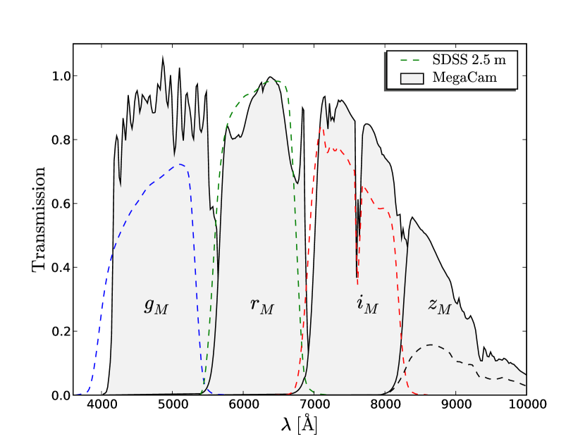
The transmission of the MegaPrime filters were characterized by their respective manufacturers and the CFHT team upon reception. Their most salient feature is the significant spatial non-uniformity of their transmission curves (namely of their central wavelength), which impacts significantly the observations (see §6). Interestingly, the new $i_{2M}$ filter exhibits a variation pattern similar to the old one, although different manufacturers produced them.

Systematic differences were found between the MegaCam and SDSS filters, which translate into small color terms between both instruments (see appendices B and G). In particular, the $u_{M}$-band filter is significantly bluer than its SDSS counterpart. This is a deliberate design choice as the MegaCam E2V chips are much more efficient in the blue than the SITe CCDs used in the SDSS imager. For this reason, the $u_{M}$-filter is sometimes labeled $u^{\star}$, in order to distinguish it from a standard $u^{\prime}$ filter.

The shutter is made of a half disk (1 meter in diameter) whose rotation is controlled precisely, in order to ensure a constant speed when the shutter crosses the CCD mosaic. The minimum exposure time that can be obtained is of 1 second, with uniformity of illumination of the large focal plane better than 10 ms. In order to increase the accuracy of the short exposure times, the exact duration of the exposure is measured with a 1 millisecond accuracy using a dedicated system independent from the shutter motion controller.

MegaPrime is operated and maintained by the CFHT team, which has steadily improved the performance of the imager. From the first light, MegaPrime images appeared to suffer from an image quality (IQ) degradation of 0.25″ (FWHM) from center to corner. For example, the mean image quality of the $r_{M}$-band exposures was 0.65″ at the center of the focal plane, and almost 0.9″ on the corners. Despite an optimization of the vertical position of the four-lens wide field corrector (WFC), this situation prevailed until November 2004, when the almost flat WFC L3 lens was flipped during an investigation. This resulted in a dramatic improvement of the IQ uniformity, with no degradation of the median IQ. In July 2005, a small tilt was applied to the camera itself resulting in an essentially uniform image quality. Exposures with IQ varying from 0.4″to 0.48″across the field of view have been routinely obtained since then. A summary of the main modifications of the imager setup is presented in table 5.

3 The SNLS Survey

The SNLS survey is a ground-based supernova survey, aiming primarily at measuring the dark-energy equation of state parameter $w$. It has been designed to build up a sample of 500 SNe Ia in the redshift range $0.3<z<1.0$. The SNLS project has two components: a large imaging survey using MegaPrime to detect supernovae and monitor their lightcurves, and a spectroscopic survey to confirm the nature of the candidates, and determine their redshift. During its five years of operation (mid-2003 to mid-2008), the survey delivered about 100 spectroscopically identified SNe Ia per year. The cosmological measurements based on the first year dataset have been presented in Astier et al. (2006).

SNLS exploits the DEEP component of the CFHT Legacy Survey (CFHTLS), which targets four low Galactic extinction fields (see table 1 for coordinates and extinction). The data are time sequenced in $g_{M},r_{M},i_{M}$ and $z_{M}$ with observations conducted every 3-4 nights in dark time, allowing the construction of high-quality multicolor supernova light curves. Because SNLS is highly vulnerable to gaps in the supernova light curves, MegaPrime was mounted on the telescope at least 14 nights around every new moon during the course of the survey —every such observing period is called a MegaCam (or MegaPrime) run. The deep CFHTLS component comprises additional observations in the MegaCam $u_{M}$ band, which are not time sequenced, and not directly used by the SNLS. The calibration of the $u_{M}$ band data has however been included in the present work.

Table 1: Fields observed by the DEEP/SN component of the CFHTLS.

Field	RA	Dec	E(B-V) a
	(2000)	(2000)	(MW)
D1	02:26:00.00	$-04$:30:00.0	0.027
D2	10:00:28.60	$+02$:12:21.0	0.018
D3	14:19:28.01	$+52$:40:41.0	0.010
D4	22:15:31.67	$-17$:44:05.0	0.027

• (from Schlegel et al., 1998)

The CFHT Legacy Survey observations are taken in “queue service observing” (QSO) mode by the CFHT staff (Martin et al., 2002). For the SNLS, an image quality better than 1″ is required. Sometimes this constraint is relaxed to meet additional constraints on the sequencing needed to ensure a regular sampling of the supernova lightcurves. However, since the SNLS is a high-priority program, and the median seeing at CFHT (in the $r_{M}$-band) is 0.75”, the actual average IQ obtained over the four fields is about 0.96″, 0.88″, 0.84″and 0.82″in the $g_{M}\ r_{M}\ i_{M}\ z_{M}$ bands. The cumulated exposure times acquired every four nights (1125 s, 1800 s, 1800 to 3600 s, 3600 s in $g_{M},r_{M},i_{M}$ and $z_{M}$ respectively) are split into 5 to 10 individual exposures of 225 to 520 s each (see Sullivan et al. (2006)). The science exposures are dithered, in order to limit the impact of the dead areas (dead columns, gaps) on the science observations. The dithering offsets are essentially determined by the size of the gaps between the CCDs, and reach 100 pixels in x (or right ascension) and 500 pixels in y (or declination).

On average, the D1 and D2 fields are observed at an airmass of 1.2, while the D3 and D4 fields are observed at a slightly higher airmass of about 1.3.

Photometric calibration exposures are routinely taken, often at the beginning and/or the end of every potentially photometric night. The science and calibration observations can therefore be separated by a few hours, and a careful detection of the non-photometric nights must be implemented. The standard calibration program consists in 5 band observations of one Landolt (1992b) field at a time. The calibration fields also contain several standard stars from the Smith et al. (2002) catalog. Since these latter standards can be bright (mag $\leq 12$), the telescope is slightly defocused, by 0.1 mm, which still allows a Gaussian PSF profile, but reduces the maximum pixel flux by about a factor two in order to avoid saturation. The exposure time of the calibration exposures is kept between two and three seconds.

All the exposures taken with MegaCam are pre-processed at CFHT by the Elixir pipeline (Magnier & Cuillandre (2004) and §5 of this paper). This pre-processing stage comprises a bias removal, a flat field correction, a photometric flat correction (see §5 and §6), and defringing of the long exposures (over 10 seconds) taken in the $i_{M}$ and $z_{M}$ bands. No defringing is applied to the calibration exposures.

Table 2: SNLS/DEEP and Landolt field observations

Field	seasons	number of epochs
		photometric / total
		$g_{M}$	$r_{M}$	$i_{M}$	$z_{M}$
D1	3.5	28 / 57	32 / 88	36 / 99	19 / 47
D2	3	13 / 44	21 / 63	25 / 66	19 / 26
D3	4	29 / 66	34 / 87	40 / 96	10 / 40
D4	4	30 / 67	34 / 97	29 / 100	19 / 55
Landolt a	–	313	311	283	240

• all Landolt (1992b) fields taken together (two to three Landolt fields may be observed each night).

This paper relies on the first 3.5 years of the survey – from August 2003 to December 2006. Table 2 shows the number of seasons and epochs for each field. It also presents the number of photometric nights, as will be discussed in §11. As will be shown below, the large number of observations allows us to implement a very robust calibration procedure, and reach low levels of internal systematic uncertainties.

4 Photometry

SNLS aims ultimately at assigning magnitudes to supernovae. In practice, this means that we have to measure ratios of supernovae fluxes to standard star fluxes. The measurement of these ratios is carried out in two steps : the ratio of (secondary) standards to science field stars (i.e. tertiary standard candidates), and the ratio of supernova to field stars. In order to be optimal, faint supernovae should be measured using PSF photometry, and hence the ratios of SN to tertiaries will be a ratio of PSF fluxes, in the same exposure. This measurement is not in the scope of this paper, and we refer interested readers to Astier et al. (2006); Guy et al. (2009).

Because we have a large number of epochs and several images per epoch, the ratio of standard fluxes to science field star fluxes is not photon-noise limited and can therefore be measured using aperture photometry. This avoids the shortcomings of PSF flux ratios over different images, with different PSFs. In this section, we describe the aperture photometry algorithm and discuss systematics affecting the ratio of standards to field star fluxes.

4.1 Aperture Photometry

Figure 2: Value of the bright star Gaussian moments as a function of the radial distance to the focal plane center. Black circles: Gaussian moments, computed on a $r_{M}$-band image, taken in 2003-10-31 (before the L3-flip). Red triangles: Gaussian moments, computed on a $r_{M}$-band image of identical seeing (at the center of the focal plane), taken two years later on 2003-10-31. As can be seen, the uniformity of the image quality has been noticeably improved.

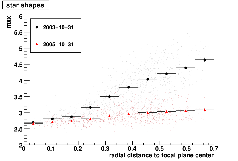
The calibration and science data is reduced using the SNLS standard reduction software used in Astier et al. (2006). Each exposure file is split into 36 smaller FITS images each corresponding to a CCD. On each smaller CCD-image, we detect the sources and model the sky background using the SExtractor package (Bertin & Arnouts, 1996). We recompute the sky background map, using only the pixels not affected by the detected object fluxes. We subtract this new background map from the image. We recompute the object Gaussian moments and aperture fluxes.

Figure 2 show the Gaussian second moments of the field stars as a function of the position on the mosaic for a $r$-band image taken in 2003 and a $r$-band image taken in the same conditions, in 2005. It is apparent from this figure that the uniformity of the PSF has improved over the course of the survey. However, given the variations of the image quality across the mosaic, we scale the photometry apertures with an estimate of the local image quality, in order to try and minimize the spatial variations of the aperture corrections.

The image quality on each CCD is estimated as the radius of the circle that has the same area as the ellipse defined by the average star second moments. We carry out the aperture photometry in a set of 10 (IQ scaled) radii (typically from 5 to 30 pixels) of all the objects detected. The apertures are centered on the positions obtained from the Gaussian fit. Tests on synthetic data demonstrated that our aperture photometry code gives accurate estimates of fluxes and errors.

Aperture pollution by neighbor objects can bias the flux estimations. We therefore chose to work with smaller apertures of radius equal to $7.5\times$ HWHM (14 pixels on average). This leads to non-negligible aperture corrections, of at least 3%. This is perfectly acceptable, as long as we check that these aperture corrections (1) are uniform across the focal plane and (2) are the same at the per mil level on the science and calibration exposures.

To check that the scaling aperture strategy gives a uniform photometry, we studied the ratio of the flux within the standard aperture adopted for the calibration studies (7.5 HWHM) over the flux computed in a much larger aperture (20 HWHM)

Figure 3: Ratio of the flux computed in two apertures of different sizes (7.5 HWHM and 20 HWHM) as a function of the image quality computed for each CCD, for a set of $r_{M}$-band images taken on 2003-10-01, when the PSF was not uniform over the focal plane. As can be seen, the ratio is not sensitive to the image quality, and hence, on the focal plane position.

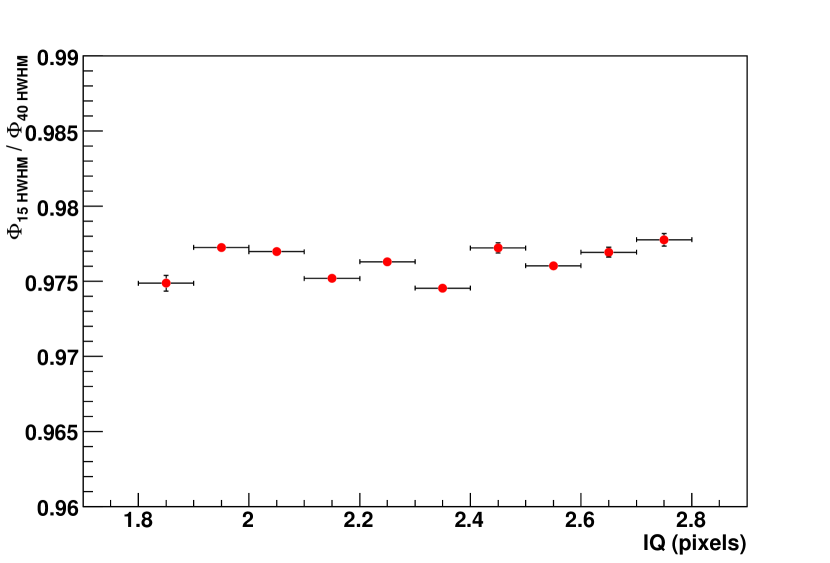
This shows that capturing a constant fraction of the flux of stars at the per mil level across the mosaic is not straightforward. There is a benefit for scaling apertures, but this approach is not sufficient for excellent quality photometry, in terms of systematic errors. We however settled for scaling apertures, using an aperture of 7.5 seeings (RMS) in radius, which makes the aperture size an issue at the 0.2% level.

4.2 Background Estimation

The “underlying background” is the sum of all the underlying sources of photons which do not come from the star itself –sky background, mainly, plus undetected objects. It is subtracted directly from the pixels using a background map computed by SExtractor. An incorrect background subtraction may bias the flux estimations, and this bias varies quadratically with the aperture radius. In order to estimate the quality of the background measurements, we chose to study the variation of the aperture corrections in a large annulus around isolated stars as a function of the star fluxes, and measure how these corrections extrapolate to very low flux. The residual background measured is $+0.06(0.003)$, $-0.03(0.006)$, $-0.23(0.03)$ and $-0.04(0.02)$ ADU per pixel in the $g_{M},r_{M},i_{M}$- and $z_{M}$-bands respectively. In the $g_{M}$- and $r_{M}$-bands, the impact of the residual background on the aperture magnitudes reported is smaller than 0.001 mag up to mag 21. Idem in the $z_{M}$-band up to mag 19. In the $i_{M}$-band, however, it induces a sizeable magnitude dependent effect, reaching 0.005 mag at magnitude $21$. However, since the measurement of the residual background on a night basis is affected by large statistical uncertainties, we chose not to correct for this effect, and include it in the systematic uncertainty budget (§12).

4.3 Aperture Corrections

The tertiary stars in science frames are calibrated with respect to observations of standard star fields. Although in both kinds of frames the fluxes are measured using aperture photometry, there is a possibility that the fraction of the flux within the aperture in both cases be different. Indeed, standard exposures are typically 2-3 seconds, without guiding, and with a telescope slightly defocused, while science exposure are integrated for 300 to 500 seconds, with guiding. In addition, there is evidence that the telescope is still vibrating when taking the standard star exposures. As a consequence, the PSF on each dataset is expected to be different, leading to different aperture corrections.

To address this issue, we computed the fractional increase of flux of sufficiently isolated objects in an aperture twice as large (12 HWHM) as the one chosen for calibration purposes (7.5 HWHM). This large aperture is considered here as an acceptable proxy for the total flux, because we expect that the PSF shape at large radii becomes increasingly independent of atmospheric variability and guiding. This flux increase is averaged over all measurements of a given night, separately for science and standard images, and separately for each band. Only nights where both science and standards were observed enter in these averages. These averages are refered to as aperture corrections, although fluxes are not “corrected”. We report in table 3 the average and r.m.s of these aperture corrections together with statistics of the image quality. One can note that aperture corrections differ only by 0.2% between science and standard frames, and are well correlated over the same night. This difference is small and is probably due to standards being observed on average with a poorer image quality. These differential aperture corrections are about 0.2 % for $g$,$r$,$i$ and $z$ bands, and compatible with 0 for $u$ band, where the image quality is on average identical for science and standard fields. This effect is accounted for by correcting the tertiary standard calibrated magnitudes, as discussed in §12.

Table 3: Statistics of the average aperture corrections and image quality over nights when both science and standards were observed. The correlation coefficients (last column) are computed for data taken over the same night in the same band.

	science		standards		$\rho_{sci,std}$
	average	r.m.s	average	r.m.s
AC	2.34%	0.55%	2.10%	0.59%	0.66
IQ	0.89″	0.2″	0.99″	0.30″	0.42

5 The Elixir Pipeline

At the end of each MegaPrime run, master twilight flat field frames and master fringe frames are built from all the exposures taken during the run, including non-CFHTLS data (which represents about half of the total dataset). The Elixir pipeline, developed and operated by the CFHT team (Magnier & Cuillandre, 2004), builds master flat fields for each filter by stacking the individual flat field frames. Individual frames inadvertently contaminated by clouds or nearby moon light are rejected. They are identified by dividing each individual flat field exposure by the master flat, and inspecting the result visually. Typically, no more than one iteration is needed to reject the outliers. In order to mitigate possible non-linearity residuals at the sub-percent level, individual flat field images are acquired in the 10,000 to 15,000 ADU range. After two weeks, there are typically 40 to 60 usable frames that can be stacked into a final normalized frame equivalent to a single 400,000 ADU counts per pixels, reducing to negligible photon noise levels (between one and two per mil).

If one measures the photometry of the same star on an image flatfielded from the twilight flats, the flux varies by about $15\%$ in the $u_{M}$ band and $10\%$ in the $g_{M}$-, $r_{M}$-, $i_{M}$-, and $z_{M}$-bands when moving the star from center to edges of the field of view. The variation is monotonic and essentially follows a circular pattern. A photometric flat, which ought to deliver uniform photometry across the field of view (see below and §6) is then created by multiplying the master flat frame by the maps of the imager photometric response non-uniformities. This frame is the one used for flatfielding the science images of the entire run, and allows for all multiplicative effects in the image to be corrected at once. The photometric flat was expected to correct this to within a percent. §6 will reveal that this is not the case, with 4% peak-to-peak residuals remaining.

Fringe patterns are built by processing all $i_{M}$- and $z_{M}$-band images corrected by the final flat. First the sky background is mapped at a large scale (100 pixels) and subtracted. Then, the exposures are scaled according to the fringe amplitudes measured on 100 peak-valley pairs on each CCD. Since all CCDs see the same sky, a single scaling factor is derived from the 36 CCDs. The scaled exposures are stacked, and an iterative process similar to the one described above is carried out, with a visual control allowing the rejection of frames containing extended astrophysical sources such as large galaxies. Note that the fringe pattern contains the signature of the photometric grid.

After these steps, Elixir processes all the images of the run, and derives an astrometric solution per CCD only, at the pixel scale level (0.2”) – no global solution over the mosaic is computed. The goal is to provide the users with a first order astrometric solution. Following this step, all the frames containing Smith et al. (2002) standards are identified and processed, with the SExtractor package (Bertin & Arnouts, 1996). The flux of the Smith et al. (2002) standard stars using the SExtractor bestphot algorithm. A median zero-point for the entire run is derived for each filter, since it is not reasonable time wise to obtain enough Smith et al. (2002) standard star observations per night to derive solid zero-point solutions. Again, the intention is to provide users with a photometric scaling, but SNLS uses its own procedures to calibrate the images, as the default calibration is not precise enough for our needs.

5.1 Plate Scale Variations

Plate scale variations cause a variation of the photometric response on images flat-fielded using twilight images (or any kind of isotropic illumination), because twilight images encode both sensitivity variations and variations of the solid angle subtended by the instrument pixels. To correct this photometric distortion introduced through flat fielding by plate scale variations, it is common to resample images on a iso-area projection prior to photometry, ignoring the Jacobian of the geometrical transformation in the course of the resampling. As this approach assumes that the only source of photometric non-uniformity of flatfielded images is the plate-scale variation, we should compare plate-scale variations and photometric non-uniformity. Note however that SNLS photometric reductions do not involve any resampling on iso-area projections.

Figure 4: Pixel area variations (i.e. square of the plate scale variations) computed on the MegaCam focal plane. Each grid rectangle corresponds to one CCD. CCD #0 is up left. CCD #35 is down right. Each CCD has been divided into $4\times 9$ superpixels. The reference superpixel  is located on CCD#13, close to the center of the focal plane. On the edges of the focal plane, the solid angle subtended by a pixel can be up to 4% smaller than on the center. Hence, due to this effect, the instrumental flux of a star measured on the edges, is at least 4% higher than the instrumental flux of this same star, measured in the same conditions on the center of the mosaic. Note that the non-uniformities actually measured on dithered exposures of dense fields (§6 and appendix A) are about 3 times larger. This indicates that the flatfield exposures taken during twilight are affected by stray light, absent from the stars’ light.

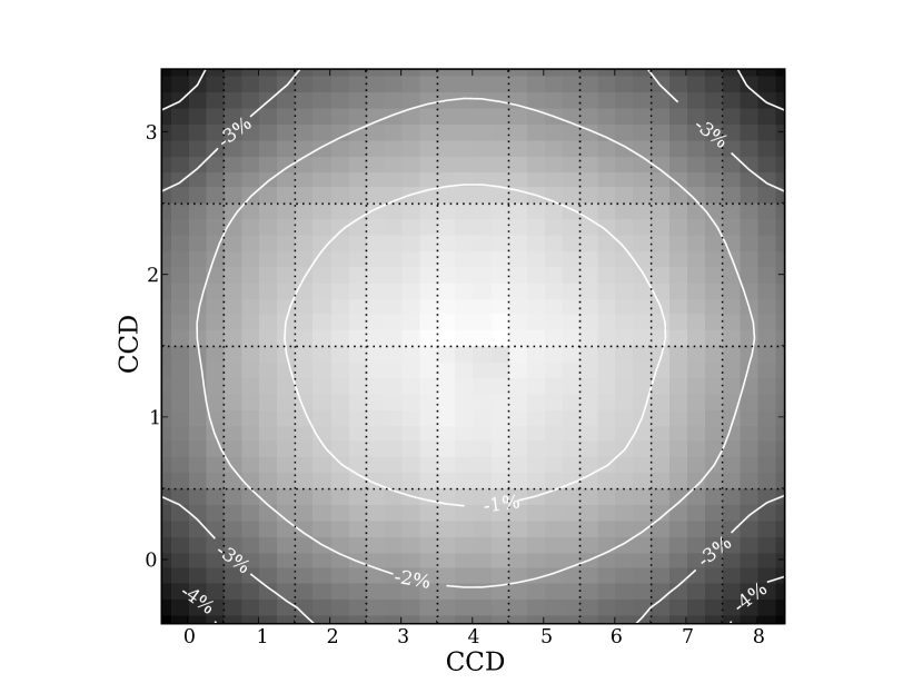
The plate scale can be determined with a precision better than 1 ‰ from the astrometry of dense stellar fields:

$$\left|\frac{\partial\omega}{\partial x\partial y}\right|=\frac{1}{\cos\delta}\times\left|\frac{\partial(\alpha\delta)}{\partial(xy)}\right|$$ (1)

where $\partial\omega/\partial x\partial y$ is the solid angle subtended by one pixel, $\alpha$ and $\delta$ refer to (e.g.) equatorial coordinates on the sky, and $x$ and $y$ are pixel coordinates on CCDs.

Figure (4) shows the variations of $\left|{\partial xy}/\partial\omega\right|$ on the focal plane, relative to a point located on CCD #13, close to the center of the camera. The pixel area scale can be up to 4% smaller on the focal plane corners than on the center. Since this variation is far smaller than the variation of photometric response we measure ($\sim 10-15\%$), we should conclude that most of the photometric non-uniformity is not due to plate scale variations.

The measured plate scale variation pattern is similar in all bands and seems to be extremely stable. It was not affected by the substantial changes of the imaging system : we have compared plate scales measured on semester 2003B and 2006B and found them to be identical at the 1‰-level.

5.2 Elixir strategy

The residual non-uniformity of photometric response is likely to be due to some source of light hitting the focal plane that does not follow the normal light path that forms a star image. This “extra” light is called “scattered light” in Elixir parlance. This name remains although the elimination of genuine sources of scattered light by extra baffling added in MegaPrime did not change the overall shape of twilight images.

It is however not necessary to identify the source of photometric response variations across the field of view to correct it. The pragmatic approach of the Elixir team has been to measure as precisely as possible the non-uniformity of the photometric response and include a correction in the flat-field images applied to the raw images. This choice has two consequences. First, images flat-fielded this way have a spatially varying sky background. Second, the 4% response variation expected from plate-scale variations is corrected for in the flat-fielding and users resampling images should account for the Jacobian of the resampling transformation prior to photometry, in order to preserve fluxes across the resampling.

The key data to measure the photometric response is a set of dithered exposures on low Galactic latitude fields, also called the “photometric grid” by the Elixir team. Elixir has implemented a reduction of these data sets and the resulting correction maps are incorporated into the flat-fields. Since the goal of the SNLS is to calibrate the imager with a sub percent precision, we have decided to put the Elixir pipeline results under scrutiny and to redetermine independently the grid correction maps applied to the data.

6 The Photometric Grids

The photometric response non-uniformity maps are derived from dithered observations of the two dense fields listed in table 4. The dithered sequence starts with an exposure followed by a series of 6 offset observations in the X direction and 6 in the Y direction. The steps increase logarithmically from a few hundred pixels up to half a mosaic. Such observations are performed almost each semester, and after each significant change in the optical path. Table 5 lists all the datasets taken since the beginning of the survey, along with the improvements of the optical path performed by the CFHT team. In order to limit the shortcomings of extinction corrections, observations are carried out in a single sequence and over a limited airmass range (typically 0.01 or less). This data is refered to as “grid observations” in the Elixir parlance, and the corrections derived from them are called “grid corrections”.

Table 4: The dense stellar fields observed to model the imager non-uniformities (Grid Fields).

Name	RA	DEC
Grid-1	06:30:00.00	14:20:00.0	winter field
Grid-2	20:00:00.00	10:00:00.0	summer field

Table 5: Grid field observations and MegaCam/MegaPrime optical improvements.

Semester	Date	Field	band
2003B	2003-10-02	Grid-2	$r_{M}i_{M}$
	2003-10-23	Grid-2	$u_{M}g_{M}z_{M}$
	2003-10-24	Grid-2	$i_{M}r_{M}$
2004A	2004-02-25	light baffle installed
	2004-03-19	Grid-1	$u_{M}g_{M}r_{M}i_{M}z_{M}$
2004B	2004-12-03	L3 Lens flipped upside-down
	2004-12-03	Grid-1	$g_{M}r_{M}i_{M}$
	2004-12-11	Grid-1	$u_{M}g_{M}z_{M}$
2004A	2005-07-20	Spacer moved (5.5 mm to 2.1 mm)
2005B	2005-09-20	Focal plane tilt tweaked
	2005-10-10	Grid-2	$u_{M}g_{M}r_{M}i_{M}z_{M}$
2006B	2006-09-13	Grid-2	$i_{M}$
	2006-09-14	Grid-2	$r_{M}$
	2006-09-15	Grid-2	$z_{M}$
	2006-09-16	Grid-2	$u_{M}$
	2006-09-19	Grid-2	$g_{M}$
2007A	2007-03-21	Grid-1	$r_{M}$
	2007-03-22	Grid-1	$u_{M}g_{M}$
	2007-03-23	Grid-1	$i_{M}$
	2007-03-24	Grid-1	$z_{M}$
2007B	2007-10-18	Grid-1	${i_{M}}_{2}$
	2007-11-08	Grid-1	${i_{M}}_{2}$
	2007-11-11	Grid-1	$r_{M}$
	2007-11-12	Grid-1	$g_{M}$

The grid exposures are processed with the standard Elixir procedure, except that no photometric flat is applied to the pixels. The instrumental fluxes of the grid stars are therefore affected by the 10% to 15% non-uniformities we are trying to model.

The data is reduced using the standard SNLS reduction procedure described below (4.1). In particular, we filter the detected objects on each individual exposure, selecting isolated star-like objects. In the $r_{M}$-band, this leaves us with $\sim 1200$ usable flux measurements per CCD. For a whole grid sequence (13 dithered observations), this represent about 100,000 stars measured twice or more, and about 600,000 flux measurements.

6.1 The Photometric Response Maps

Our goal is to determine how the instrumental magnitudes of a star vary as a function of the position on the focal plane. In practice, it is convenient to choose a specific location as the reference location, ${\mathbf{x}}_{0}$, and the relation between the instrumental magnitudes of an object, at positions ${\mathbf{x}}$ and ${\mathbf{x}}_{0}$, $m_{ADU|{\mathbf{x}}}$ and $m_{ADU|{\mathbf{x}}_{0}}$ can be parametrized as:

$$m_{ADU|{\mathbf{x}}}-m_{ADU|{\mathbf{x}}_{0}}=\delta zp({\mathbf{x}})+\delta k({\mathbf{x}})\times{\rm col}_{|{\mathbf{x}}_{0}}$$

where ${\rm col}$ is some color of the star. The maps $\delta zp({\mathbf{x}})$ and $\delta k({\mathbf{x}})$ are determined from the grid observations, and account for the non-uniformities of the imager. By definition, these maps vanish at the reference location: $\delta zp({\mathbf{x}}_{0})=0$ and $\delta k({\mathbf{x}}_{0})=0$. Physically speaking, $\delta zp({\mathbf{x}})$ encodes the spatial variations of the overall integral of the bandpass, while $\delta k({\mathbf{x}})$ encodes (at first order) the variations of its central wavelength. In what follows, “passband variations” refer to variations of the passband shape irreducible to an overall constant. If the imager passbands are uniform over the focal plane, we expect $\delta k({\mathbf{x}})$ to be zero everywhere. Conversely, if the imager passbands do vary as a function of the position, we should measure a non-zero color term between positions ${\mathbf{x}}$ and ${\mathbf{x}}_{0}$.

The quantity ${\rm col}_{|{\mathbf{x}}_{0}}$ is the star color, measured in the MegaCam passbands at the reference location. There is some degree of arbitrariness in the definition of ${\rm col}_{|{\mathbf{x}}_{0}}$, since it is always possible to redefine the color reference ${\rm col}\rightarrow{\rm col}+\Delta{\rm col}$, and absorb the difference in the $\delta zp({\mathbf{x}})$’s: $\delta zp({\mathbf{x}})\rightarrow\delta zp({\mathbf{x}})-\delta k({\mathbf{x}})\times\Delta{\rm col}$. Hence, there is a color convention associated with each $\delta zp({\mathbf{x}})$ map, which must be made explicit. We choose to define a conventional grid reference color, ${\rm col}_{grid}$, and parametrize the grid corrections as:

$$m_{ADU|{\mathbf{x}}}-m_{ADU|{\mathbf{x}}_{0}}=\delta zp({\mathbf{x}})+\delta k({\mathbf{x}})\times\Bigl{[}\ {\rm col}_{|{\mathbf{x}}_{0}}-{\rm col}_{grid}\Bigr{]}$$ (2)

There are several ways to choose the grid reference colors. One possibility is to define them as the mean color of the grid stars, in order to minimize the statistical uncertainties carried by the $\delta zp({\mathbf{x}})$ maps. Another way is to choose them close to the colors of the science objects under study. This way, the instrumental magnitudes of these objects, once corrected by the $\delta zp({\mathbf{x}})$ maps would be almost uniform on the focal plane. We must note however, that the grid reference colors are just internal quantities, that do not affect the definition of the tertiary magnitudes.

In the next section, we detail how we extract the $\delta zp({\mathbf{x}})$ and $\delta k({\mathbf{x}})$ maps from the grid data.

6.2 Measuring the Photometric Response Maps

As described in section 5 the grid data in one MegaCam band consists in 13 dithered observations of a dense stellar field (about 100,000 isolated stars per exposure). Each field star being observed at various locations on the focal plane, one can compare the instrumental magnitudes at those locations and fit the $\delta zp({\mathbf{x}})$ and $\delta k({\mathbf{x}})$ maps defined in the previous section.

To parametrize the grid maps, we chose to develop them on basis functions: $\delta zp({\mathbf{x}})=\sum_{k}\alpha_{k}p_{k}({\mathbf{x}})$ and $\delta k({\mathbf{x}})=\sum_{k}\beta_{k}q_{k}({\mathbf{x}})$. Since the photometric response variations may be sharp, especially when transitioning from one CCD to another, we used a basis of independent superpixels (also called cells thereafter), rather than smooth functions such as splines or polynomials. To model the $\delta zp({\mathbf{x}})$ map, we divided each CCD into $N_{x}\times N_{y}=4\times 9$ superpixels. Each superpixel is $512\times 512$ pixels wide and contains about 70 bright, isolated grid stars, which is enough to measure the $\delta zp({\mathbf{x}})$ with a precision better than 0.001 mag. We have found that determining the $\delta k({\mathbf{x}})$ requires more stars per superpixel, in order to have a sufficient color lever-arm in each cell. We therefore used larger cells, dividing each CCD into $N_{x}\times N_{y}=2\times 3$ cells.

With such a parametrization, the number of grid parameters is $4\times 9\times 36+2\times 3\times 36-2=1510$, one cell being taken as a reference for each map. Fitting such a model (i.e. building and inverting a $1510\times 1510$ symmetric positive definite matrix) is routinely done on modern desktop computers.

With only 13 dithered exposures, about 99% of the grid stars are never observed on the reference cells. Hence the instrumental magnitudes of these stars at the reference location, $m_{ADU|{\mathbf{x}}_{0}}$, are never directly measured and must be fitted along with the grid map parameters. The same is true for the star colors ${\rm col}_{|{\mathbf{x}}_{0}}$, which means that we must analyze the grid data in two bands simultaneously. This adds about 200,000 (nuisance) parameters to the fit, turning it into a large dimensionality, non-linear problem, which is much more difficult to solve.

In order to make the problem tractable, we have followed an iterative approach, after checking with simulations that this is feasible. In the first step, we fit the data independently in each band, ignoring the $\delta k({\mathbf{x}})\times{\rm col}$ terms. We then update the star colors, and refit the grid data in each band. We have found that it suffices to iterate the procedure twice in order to retrieve the correct colors. No such iterative procedure applies for the star magnitudes though. Fitting 100,000 parameters is still possible, using approximate methods, which do not require to build the $\chi^{2}$ second derivative matrix, such as the conjugate gradient method. It is also possible to fit alternatively one set of parameters, keeping the other ones fixed. We have experienced however, that the conjugate gradient method converges very slowly and can lead to wrong solutions, if one is not ready to perform the $O(100,000)$ required iterations. Successive optimizations on the grid parameters at fixed star magnitudes, and vice versa also converge very slowly and remain far from the true minimum.

Fortunately, we have found that the structure of the problem is simple enough to allow us to obtain the true minimum of the $\chi^{2}$, and determine simultaneously the grid parameters, the grid star magnitudes, along with their exact covariances. The details of the method are documented in details in appendix A. The approach in fact applies to many other calibration problems, such as least squares for astrometric solutions as posed in e.g. Kaiser et al. (1999); Padmanabhan et al. (2008). In the remaining of this section, we will present the results obtained with this technique.

6.3 Monte-Carlo Checks

The extraction technique described in appendix A was tested on simulated data. Our main concern was to look for possible degeneracies affecting the determination of the grid correction parameters, as well as possible biases, coming from the fact that the fit is slightly non-linear.

A realistic catalog of grid stars was built from real $r_{M}$- and $i_{M}$-band measurements. Using this catalog, a photometric distortion model and the dithering pattern applied to the grid sequence, we generated a hundred realizations of a typical two-band grid run. From this set of data, the grid corrections, $\delta{zp}({\mathbf{x}})$ and $\delta{k}({\mathbf{x}})$ were reconstructed from each realization and compared to the photometric distorsion model.

Figure 5: Top panel: normalized distribution of the difference between the reconstructed and simulated $\delta{zp}({\mathbf{x}})$ parameters, for 100 realization (filled histogram) and 1 single realization (unfilled histogram). The reconstructed grid parameters are globally affected by the uncertainty of the reference cell zero point (see section 6.3). Bottom panel: difference of the reconstructed and simulated grid parameters as a function of the cell number, for a single realization. No spatially dependent effect can be detected.

Figure 6: Top panel: distribution of the difference between the reconstructed and simulated $\delta k$ parameters, for 100 realization (filled histogram) and 1 single realization (unfilled histogram). The reconstructed grid parameters are globally affected by the uncertainty of the reference cell zero point (see section 6.3). Bottom panel: difference of the reconstructed and simulated grid parameters as a function of the cell number, for a single realization. No spatially dependent effect can be detected.

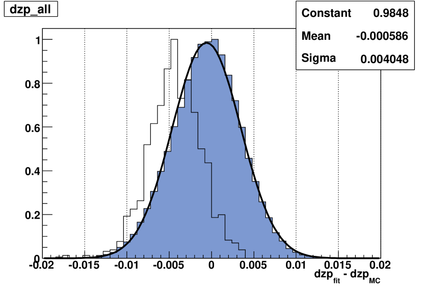
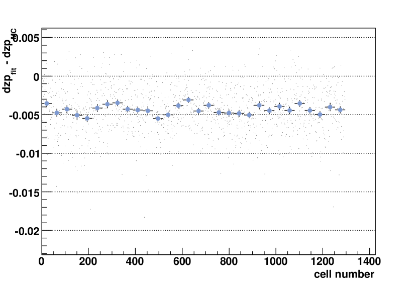
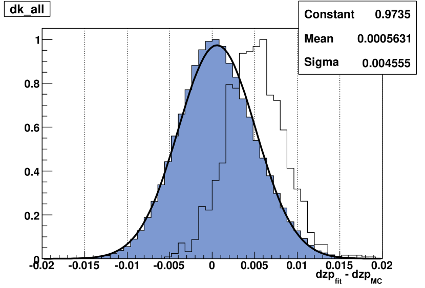
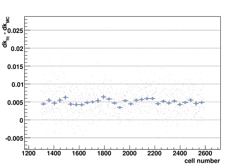
Figures (5) and (6) show the distribution of the difference between the simulated photometric distorsion model and the reconstructed grid calibration parameters, in the $i_{M}$-band, for all the 100 realization processed. It is clear from those figures that the extraction method is an unbiased estimator of the photometric distorsion model, as could be expected from a (almost) linear fit.

On the same figure, we have represented the same difference, obtained for one realization only. We see that the reconstructed grid correction parameters are offset by a small amount, and the value of the offset is almost exactly opposite for the $\delta{zp}({\mathbf{x}})$ and the $\delta{\lambda}({\mathbf{x}})$. This effect comes from the structure of the noise affecting the $\delta{zp}({\mathbf{x}})$ and $\delta{k}({\mathbf{x}})$ map estimates. All the $\delta{zp}({\mathbf{x}})$ (resp. $\delta{k}({\mathbf{x}})$) are positively correlated with a correlation coefficient of about $0.5$. These values can be easily explained if we consider that each $\delta{zp}$ (resp. $\delta{k}_{i}$) cell value is the difference between the the zero point (resp. color term) of cell number $i$ and the zero point (resp. color term) of the reference cell.

Robustification algorithms have been implemented in the fit procedure: the fit was performed several times, and at each cycle, the measurements with a partial $\chi^{2}$ above 4 sigmas of the median $\chi^{2}$ were removed. This is unavoidable, since least-square methods are extremely vulnerable to outliers, and since we are dealing with $10^{5}-10^{6}$ measurements, potentially affected by undetected cosmics or bad pixels. We have checked the robustification scheme by generating 2% of outliers in the simulated dataset. The error affecting the outliers was chosen uniform in the $[-2{\rm mag};+2{\rm mag}]$ range. The results presented in figures (5) and (6) show that the robustification procedure correctly rejects the outliers.

The extraction method described above ignores possible variations of the atmospheric absorption during one dithering scan. Since such variations can bias the grid parameter reconstruction, it is tempting to fit, along with the grid parameters, one global zero point per exposure, in order to correct from such variations. We have implemented this model, and run it on simulated data. We have found, inspecting the covariance matrix of the fit that there is an almost total degeneracy between the grid parameters and the exposure zero-points.

Not surprisingly, the uncertainties on the reconstructed grid parameters, marginalized over the exposure zero points are much higher, of the order of several percents. Hence, the only way to deal with atmospheric absorption is to add a control exposure at the end of the sequence, similar to the first exposure. This would allow one to assess whether the sequence was photometric or not. Unfortunately, no such control exposure is currently available. One may recover an acceptable accuracy by fitting a coarser (typically one coefficient per CCD) non-uniformity model to the data. One can still be reasonably confident that the atmospheric variations do not affect the grid data. Indeed, before taking a grid sequence, the observers ensured that the conditions were indeed photometric according to the SkyProbe monitor.

Finally, it is interesting to compare the minimum $\chi^{2}$ values obtained when fitting either the grid model presented above or the same model, with all $\delta{k}({\mathbf{x}})$ parameters fixed to zero. We notice that the $\delta\chi^{2}$ between both models is of the order of 3000 (for 215 parameters added). This is a very significant improvement. However the fractional improvement on the fit residuals remains very modest: below $10^{-2}$. This shows that when dealing with such a large dimensionality problem, we can get a perfectly acceptable reduced $\chi^{2}_{min}$ for a model which is obviously wrong. Hence, obtaining the true minimum of the $\chi^{2}$ function using an exact technique such as the one presented in appendix A is vital to determine the optimal grid corrections.

6.4 Results

All the datasets presented in table 5 were analyzed with the procedure described in §6.2, 6.3 and appendix A. We parametrize the color corrections as follows:

$$g_{ADU|{\mathbf{x}}} =g_{ADU|{\mathbf{x}}_{0}}+\delta zp_{g}({\mathbf{x}}) +\delta k_{ggr}({\mathbf{x}})\times\Bigl{[}(g-r)_{|{\mathbf{x}}_{0}}-(g-r)_{grid}\Bigr{]}$$

$$r_{ADU|{\mathbf{x}}} =r_{ADU|{\mathbf{x}}_{0}}+\delta zp_{r}({\mathbf{x}}) +\delta k_{rri}({\mathbf{x}})\times\Bigl{[}(r-i)_{|{\mathbf{x}}_{0}}-(r-i)_{grid}\Bigr{]}$$

$$i_{ADU|{\mathbf{x}}} =i_{ADU|{\mathbf{x}}_{0}}+\delta zp_{i}({\mathbf{x}}) +\delta k_{iri}({\mathbf{x}})\times\Bigl{[}(r-i)_{|{\mathbf{x}}_{0}}-(r-i)_{grid}\Bigr{]}$$

$$z_{ADU|{\mathbf{x}}} =z_{ADU|{\mathbf{x}}_{0}}+\delta zp_{z}({\mathbf{x}}) +\delta k_{ziz}({\mathbf{x}})\times\Bigl{[}(i-z)_{|{\mathbf{x}}_{0}}-(i-z)_{grid}\Bigr{]}$$

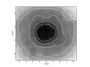
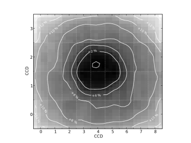
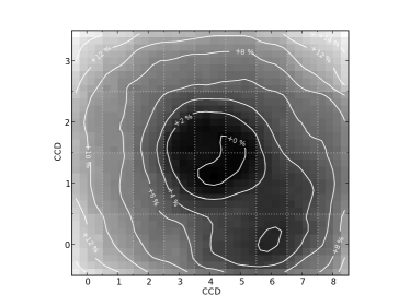
Figure 7 presents the $g_{M},r_{M},i_{M}$- and $z_{M}$-band $\delta zp$ maps obtained on the 2005B dataset, using images flat-fielded with twilight flats. In all bands, a same star will yield a higher instrumental flux if observed on the edge of the camera than if observed on the center. These maps include the plate scale variations, but display larger non-uniformities. Juramy et al. (2008) present strong evidence for internal reflections in the MegaPrime wide-field corrector which add extra light in the center of the field of view, and hence tend to explain the need for correcting twilight flats. The structure of the $\delta zp({\mathbf{x}})$ maps evolves slowly as a function of time, as shown on figure 8. This evolution is mainly due to small changes in the optical path (see table 5) and to the accumulation of metal shavings from the filter exchange mechanism on the top optical surface below the filter mechanism, due to the intense operation of the filter jukebox. This dust being somewhat shiny, it probably modified the internal reflection pattern within the optical path, corrupting the flatfields. The dust was identified and removed in January 2007, and a preventive program to monitor the cleanliness of the optical path was set up.

(a) $\delta{zp}_{g,g-r}({\mathbf{x}})$

(b) $\delta{zp}_{r,r-i}({\mathbf{x}})$

(c) $\delta{zp}_{i,r-i}({\mathbf{x}})$

(d) $\delta{zp}_{z,i-z}({\mathbf{x}})$

Figure 7: $g_{M},r_{M},i_{M}$- and $z_{M}$-band $\delta{zp}({\mathbf{x}})$ maps determined from grid observations taken in 2005. In all bands, the instrumental flux of a star, measured on the corner a flat-field corrected image, will be 10 to 15% higher than that of the same star, measured on the center of the mosaic. The plate scale variations account for about half of this effect. The other half is attributed to so-called “scattered light”, i.e. light that does not follow the normal path that form a star. In some bands, we see sharp steps between the two CCD amplifiers. These are due to the fact that the flat-field images are taken by combining all the images taken during a run, and that the gain of the amplifiers can vary by about 1% during a run.

(a) $\delta{zp}_{r,r-i}({\mathbf{x}})\ \ (2003B)$

(b) $\delta{zp}_{r,r-i}({\mathbf{x}})\ \ (2004B)$

(c) $\delta{zp}_{r,r-i}({\mathbf{x}})\ \ (2005B)$

(d) $\delta{zp}_{r,r-i}({\mathbf{x}})\ \ (2006B)$

Figure 8: $r_{M}-$band $\delta{zp}({\mathbf{x}})$ maps determined from grid observations taken from 2003 to 2007. The variations of the maps are due to metal shavings accumulating is the optical path, and modifying the “scattered light” pattern.

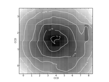
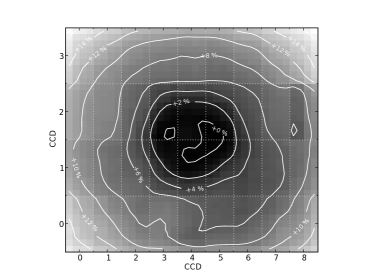
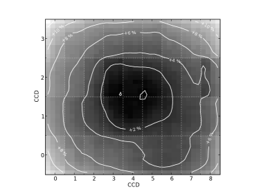
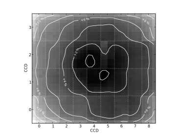
The $\delta k({\mathbf{x}})$ maps are presented in figure 9. We do measure non-zero color terms between the reference location and any other focal plane location. This came as a surprise, and was later validated by the filter scans provided by the filter manufacturer (see §7). The non-uniformity pattern is essentially invariant by rotation around the center of each filter. This is inherently the result of the manufacturer pushing the technology when coating filters of that size ($300{\rm mm}\times 300{\rm mm}$) with multiple layers. The coating chambers simply do have a projection beam uniform enough to deliver the uniformity routinely achieved on smaller filters. The $\delta k({\mathbf{x}})$ maps were determined independently on each grid set. No significant variations of the maps were found between 2003 and 2006.

The reduced $\chi^{2}_{\rm min}$ obtained from the fits is of about 4 in the $g_{M}$-band and 3 in the $r_{M},i_{M}$ and $z_{M}$-bands. Indeed, we have neglected the contribution of the flat field errors and of the fringing when evaluating the photometric measurement uncertainties. Since the fit is linear, we have chosen to re-scale the photometric errors by the appropriate amount, in order to obtain $\chi^{2}_{\rm min}/{\rm ndof}\sim 1$, and to renormalize the covariance matrix of the grid corrections accordingly.

The statistical uncertainties affecting the $\delta zp({\mathbf{x}})$ are of a little less than 0.001 mag in all bands. This uncertainty level is comparable to the photon noise affecting the bright star instrumental magnitudes. The statistical uncertainties on the $\delta k({\mathbf{x}})$ maps are of about 0.002 mags in all MegaCam bands. At the chosen grid reference color, they are slightly correlated with the $\delta zp({\mathbf{x}})$ maps with a correlation coefficient of $-0.25$. We have checked that, in all bands, the statistical uncertainty introduced by the grid corrections on the magnitudes transformed to the reference location is never larger than 0.002 mag for stars of colors $g_{M}-r_{M}<1.0$, and of about 0.003 for stars of $g_{M}-r_{M}\sim 1.5$.

   

(a) $\delta k_{g,g-r}({\mathbf{x}})$

(b) $\delta k_{r,r-i}({\mathbf{x}})$

(c) $\delta k_{i,r-i}({\mathbf{x}})$

(d) $\delta k_{z,i-z}({\mathbf{x}})$

Figure 9: $g_{M}$-, $r_{M}$, $i_{M}$- and $z_{M}$-band $\delta k({\mathbf{x}})$ maps determined from grid observations taken in 2005. In all bands, we observe a radial pattern, which is well reproduced using synthetic photometry and filter scans provided by the filter manufacturer (REOSC), as will be shown in §7.3. The contour lines are displayed to allow the reader to estimate the amplitude of the passband variations.

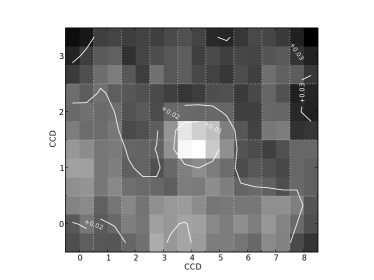
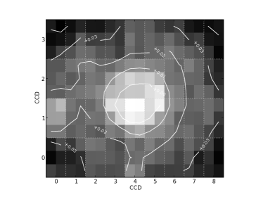
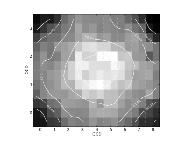
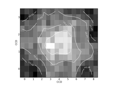
The fact that the imager passbands depend on the focal plane position has important consequences on the calibration scheme. In particular, a significant part (up to 1-2%) of the uniformity corrections depend on the color of each object. We will detail how we account for the grid corrections in section 6.6.

6.5 Comparison with Elixir findings

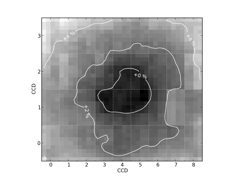
The Elixir analysis of the grid data did not find significant color terms and solved for the $\delta zp({\mathbf{x}})$ without $\delta k({\mathbf{x}})$ terms and did not solve for star magnitudes. The results are hence significantly different : the $\delta zp({\mathbf{x}})$ maps re-analyzed by the SNLS collaboration span a range larger by about 0.04 mag than the ones found by Elixir, as shown on figure 10. We found that the residual non-uniformity pattern observed on the Elixir processed images is not constant and varies from one grid observation set to another. The discovery of these non-uniformities triggered the reanalysis of the grid dataset described above.

Up to the T0006 CFHTLS release (spring 2009), data were processed using the standard Elixir recipe. The uniformity corrections presented in the previous section will be integrated in 2009 after further interactions with the Elixir team and the CFHTLS users community. This is planned for the final release of the CFHTLS data T0007 (spring 2010).

Figure 10: Residual non-uniformities measured on a set of grid exposures taken during semester 2004B, and processed with Elixir, using the photometric correction maps in use for releases T0004.

6.6 Applying the Grid Corrections to the Data

Because the grid corrections are color dependent, it is impossible to obtain uniform instrumental magnitudes for all objects. In practice, we have chosen to apply the $\delta zp({\mathbf{x}})$ maps directly to the instrumental star magnitudes, defining so-called “hat-magnitudes”:

$$\hat{g}_{ADU|{\mathbf{x}}} = g_{ADU|{\mathbf{x}}}-\delta zp_{g}({\mathbf{x}})$$

$$\ldots$$

$$\hat{z}_{ADU|{\mathbf{x}}} = z_{ADU|{\mathbf{x}}}-\delta zp_{z}({\mathbf{x}})$$ (3)

It would have been possible to apply them directly at the pixel level. We have chosen to deal directly with the fluxes mainly for practical reasons, as it did not imply a full reprocessing of the SNLS data.

The hat magnitudes of stars of colors equal to the grid reference colors are uniform across the focal plane. The hat magnitudes of all other objects vary according to the relations:

$$\hat{g}_{ADU|{\mathbf{x}}} =g_{ADU|{\mathbf{x}}_{0}}+\delta k_{ggr}({\mathbf{x}})\times\Bigl{[}(g-r)_{|{\mathbf{x}}_{0}}-(g-r)_{grid}\Bigr{]}$$

$$\ldots$$

$$\hat{z}_{ADU|{\mathbf{x}}} =z_{ADU|{\mathbf{x}}_{0}}+\delta k_{ziz}({\mathbf{x}})\times\Bigl{[}(i-z)_{|{\mathbf{x}}_{0}}-(i-z)_{grid}\Bigr{]}$$ (4)

It should be pointed out once again that the definition of the hat magnitudes depend on the conventional grid reference colors, ${\rm col}_{grid}$. However, we will see in §8 and §9 that the grid color conventions are purely internal quantities and have no impact on the calibrated tertiary magnitudes.

The instrumental magnitudes entering the calibration pipeline were measured on the survey images processed with the official Elixir pipeline, which included a correction for the non-uniformities of the imager. This correction was applied at the pixel level (see above). Hence, what we measured were actually “Elixir hat-magnitudes”:

$$\hat{g}^{Elixir}_{ADU|{\mathbf{x}}} = g_{ADU|{\mathbf{x}}}-\delta zp^{Elixir}_{g}({\mathbf{x}})$$

$$\ldots$$

$$\hat{z}^{Elixir}_{ADU|{\mathbf{x}}} = z_{ADU|{\mathbf{x}}}-\delta zp^{Elixir}_{z}({\mathbf{x}})$$ (5)

As a consequence, the Elixir grid corrections had to be removed and the new $\delta zp({\mathbf{x}})$ corrections applied:

$$\hat{g}_{ADU|{\mathbf{x}}} = \hat{g}^{Elixir}_{ADU|{\mathbf{x}}}+\delta zp_{g}^{Elixir}({\mathbf{x}})-\delta zp_{g}({\mathbf{x}})$$

$$\ldots$$

$$\hat{z}_{ADU|{\mathbf{x}}} = \hat{z}^{Elixir}_{ADU|{\mathbf{x}}}+\delta zp_{z}^{Elixir}({\mathbf{x}})-\delta zp_{z}({\mathbf{x}})$$

There are basically two ways to handle the residual color corrections. We can elect a specific focal plane position (e.g. ${\mathbf{x}}_{0}$), transform all the hat magnitudes to this position, using the $\delta k({\mathbf{x}})$ maps and choose to report all the MegaCam magnitudes at this specific position. However, stars are complicated objects, and even main sequence stars do not follow linear color corrections over large color ranges, of one magnitude or more. Furthermore, non stellar objects such as galaxies or supernovae do not obey the grid corrections. Instead, we chose to leave the science object instrumental magnitudes untouched, and define a system of “local natural magnitudes”. This is possible because the ditherings applied to the survey images are small, which ensures that each object is always observed with the same effective filters. Working with natural magnitudes ensures that they can be directly converted into broadband fluxes, provided that we have a model of the telescope effective passbands at each position of the focal plane – as well as a spectrum with known magnitudes. Building such a model is the subject of §7.

The average $\delta k({\mathbf{x}})$ maps may be obtained from the CDS. The $\delta zp({\mathbf{x}})$ will be made available along with the next Elixir data release. Indeed, some further work with the Elixir team is needed, in order to decide the optimal grid reference colors for each component of the CFHT Legacy Survey and validate the new reduction procedure with a larger user base.

7 MegaCam Passbands

7.1 Transmission of the filters in the telescope beam

MegaCam filters are interference filters and exhibit a transmission depending on the crossing angle, as expected for this type of filters. We describe in this paragraph how we synthesized the transmission of the filters in the telescope beam from laboratory measurements of the filter transmissions.

We have at our disposal two kinds of laboratory measurements: a set of transmission curves measured at about a dozen of positions on the filter, all on the sides of the filters because the equipment has a limited mechanical clearance. Some of the positions were measured at 0, 2, 4 and 6 degrees from normal incidence (Benedict, private communication). The other set of measurements was provided by the filters manufacturer : it consists in a transmission curve at normal incidence at 10 positions along a radius for each filter. From the first set of measurements, we can check that the circular symmetry is an excellent approximation. We can also model the angular dependence. Assuming the circular symmetry, interpolating the other set of measurements provides us with transmission curves at normal incidence anywhere on the filters. Since filters are located at about 10 cm from the focal plane, we identify in what follows a position on the focal plane with a position on the filter.

The angular dependence of interference filters transmission can be approximated by:

$$T\left(\lambda,\theta\right)=T\left(\lambda\left[1-\frac{\sin^{2}\theta}{n^{2}}\right]^{-1/2},\theta=0\right)$$

where $n$ is the refracting index of the filter, and $\theta$ the incidence angle. This expression, exact for a single Fabry-Perrot layer, is sufficiently accurate to describe the angular dependence measured on the MegaCam filters. We find effective indices of 1.80, 1.70, 1.80, 1.60, 1.50 for $u_{M},g_{M},r_{M},i_{M}$ and $z_{M}$ respectively, with an uncertainty of about 0.1. The angular dependence of the transmission has potentially two effects: it induces a radial dependence of the transmission of a filter, even if it were perfectly uniform; secondly, it shifts towards the blue the transmission in the telescope beam compared to the laboratory measurements at normal incidence. The first effect is in fact very small for MegaCam: the mean angle of the beam changes by about 10 milliradians between the center and the corner of the mosaic, and the cut-on and cut-off wavelengths of a filter are shifted by less than a part in $10^{4}$, and cannot account for the position dependence of the transmission measured on the sky. The second effect turns out to be non-negligible in the f/4 beam at CFHT prime focus: it shifts the filter central wavelengths by a few per mil. In order to synthesize the transmission of the filters, we integrated the measurements provided by the manufacturer over the telescope beam (with central occultation), assuming the above expression for the angular dependence. If compared to normal incidence transmissions, the effective wavelengths shift to the blue uniformly across the focal plane by amounts ranging from 4 Å for $u_{M}$ band to 14 Å for $z_{M}$ band.

7.2 Effective passbands

The effective passbands combine many contributions, among which (1) the CCD quantum efficiencies (2) the filter transmissions (3) the transmission of the various lenses and windows in the optical path (4) the mirror reflectivity (5) the average atmospheric transmission at Mauna Kea as recently determined by the SuperNova Factory (SNF) Collaboration (Buton & SNfactory Collaboration, 2009) and (6) the transmission spectrum of the telluric features including the strong ${\rm O_{2}}$, ${\rm OH}$ and ${\rm H_{2}0}$ absorption features in the red and near infrared (Hinkle et al., 2003).

The effective passbands, along with their ingredients are listed in appendix B. The full electronic version of these tables can be retrieved from the CDS.

7.3 Comparison of the observed and synthetic color terms

Figure 11: Difference between the $i_{M}$ instrumental magnitude of stars located on the edge of the focal plane (ccd # 9, 17, 18 & 26) as a function of their $(r_{M}-i_{M})$ color at the reference location. The large dots are the profile of the star measurements, corrected for the $\delta zp({\mathbf{x}})$ map, the small dots are the synthetic magnitudes, computed using the Pickles (1998) library and models of the passbands at the the center of the focal plane and at 11.5 cm from the center. The line shows the average linear grid color correction $\delta k({\mathbf{x}})\times(r_{M}-i_{M})$. As can be seen, the grid color corrections are well approximated by linear relations.

Figure 12: Comparison of the color terms measured on the grid data, with synthetic ones as a function of the distance to field center. The measurement points are averages at the quoted radius, with their error bars displaying the r.m.s over the circle. The synthetic ones are computed by integrating the Pickles (1998) stellar library in the synthetic transmissions. The synthetic color terms depend only mildly on the color range and stellar types, except for the $r_{M}$ band, where the disagreement worsens with the Stritzinger et al. (2005) library.

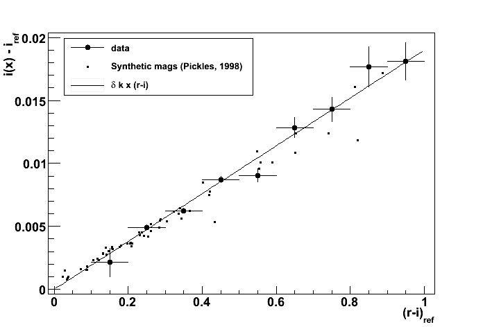
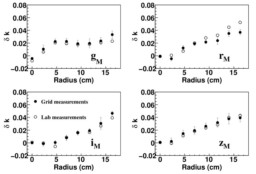
Figure 11 compares the $i_{M}$-band instrumental magnitudes of stars observed at the edge of the focal plane and at the reference location as a function of the star $(r_{M}-i_{M})$ colors. As can be seen, there is a good agreement between the synthetic magnitudes computed using the effective passband models presented in this section and the grid measurements. Note also that the effect of the filter non-uniformities is small, and well described by a linear color term. Figure 12 compares the color terms across the focal plane measured with the grid data with synthetic evaluations from the Pickles (1998) stellar library. Except for the filter itself, we used average transmissions, and in particular the average quantum efficiency curve for the CCDs.

Similar results are obtained using the Stritzinger et al. (2005) stellar library, except for the $r_{M}$ band, where the agreement becomes worse than shown here. We suspect that stellar SEDs are poorly indexed by $r_{M}-i_{M}$, and do not regard this mild disagreement (at the level of 0.01) as very serious. The fair agreement in the other bands, together with its stability with a change of stellar library is indeed a good indication of the quality of the grid solution. Taken at face value, the differences between the two sets of curves cause shifts of the zero points below the millimagnitude level for all bands (and is hence negligible) except for $r_{M}$ band where it would reach 2 millimagnitudes. We decided to ignore this potential contribution to the error budget because the synthetic $r_{M}$ color terms are very sensitive to the assumed stellar population, making the result questionable.

8 Landolt Stars

8.1 The Landolt Photometric System

The photometric catalog published by Landolt (1992b) is the most widely used standard star network. It contains $UBVRI$ Johnson-Kron-Cousins magnitudes of 526 stars centered on the celestial equator in the $11.5<V<16.0$ magnitude range. The repeatability is of about 1% in all bands resulting in magnitude uncertainties of 0.003 mag. The uniformity of the catalog is believed to be excellent, of about 1%. This standard star network was used to calibrate the broadband observations of the nearby SNe Ia used to supplement the SNLS dataset. The systematic differences between photometric systems are not well controlled and can amount to $2\%-4\%$. In order to avoid this additional source of error in the cosmological analyzes, we rely on the Landolt (1992b) standard star network to calibrate the SNLS survey.

The genealogy of the Landolt $UBV$ magnitudes can be traced back to the pioneering work of Johnson & Morgan (1951, 1953); Johnson & Harris (1954); Johnson (1955, 1963). Landolt (1973) transferred the Johnson (1963) photometric system to a set of 642 bright ($6.0<V<12.5$) equatorial stars, selected for their stability. This program was conducted at Kitt Peak National Observatory (KPNO), using the 16- and 36-inches telescopes, and a refrigerated 1P21 photomultiplier similar to that used by Johnson and collaborators. $R$- and $I$-band magnitudes were added about ten years later. The catalog published in (Landolt, 1983) gives $UBVRI$ magnitudes of 223 $7.0<V<12.5$ stars. This work was based on observations made on the Cerro Tololo Inter-American Observatory (CTIO) 0.4- and 0.9-m telescopes, using a different type of photomultiplier (RCA 31034) and slightly different filters. The $UBV$ magnitudes were tied to the Landolt (1973) system, the $RI$ band observations were tied to the system defined by Cousins (1978). Finally, Landolt (1992b) published $UBVRI$ magnitudes of 526 fainter ($11.5<V<16.0$) equatorial stars, tied to the 1983 catalog. This catalog was built from observations taken with the CTIO 0.9-m and 1.5-m telescopes, RCA 31034A and Hamamatsu R943-02 photomultipliers and the same $UBVRI$ filters used to develop the 1983 catalog. Additional papers containing photometry of particularly well-studied stars, mainly spectrophotometric standards were also published (Landolt, 1992a; Landolt & Uomoto, 2007). In particular, Landolt & Uomoto (2007) contains Landolt magnitudes of 31 stars, among which spectrophotometric standards used to calibrate the Hubble Space Telescope. Most Landolt (1992b) standards are red objects with an average $B-V$ color of $0.81\pm 0.52(rms)$. The Landolt stars observed by MegaCam are mainly located in the Selected Area (SA) fields, which contain very few blue stars. The average $B-V$ color of the Landolt stars observed with MegaCam is $0.77\pm 0.31(rms)$. As a consequence there are very few observed stars in the color range $0<B-V<0.25$.

Contrary to statements found in the literature, the Landolt system is not defined in terms of any particular magnitude of Vega, nor is the Johnson system. The absolute “gray” zero-point of the Johnson system is linked to the former “International Photovisual System” via 9 stars in the so-called “North Polar Sequence”, reobserved by Johnson & Morgan (1951). The color zero-points were set from 6 A0V stars of which Vega is one, by the condition that the average $B-V$ and $U-B$ color index of these stars is exactly zero (Johnson & Morgan, 1953). Vega and the North Polar Sequence objects were too bright for Landolt to observe, even on small telescopes. As noted above, the Landolt $R$ and $I$ magnitudes are tied to the system defined by Cousins (1976). The zero-points of this latter system are also defined so that the colors of a “typical” A0V star are all zero. However, no mention of Vega appears in Cousins (1976). Hence, there are large uncertainties on the magnitudes of Vega in the Landolt system.

It must also be noted that the Landolt system is not a natural system. The reduction procedure used to derive the calibrated magnitudes from the raw observations is described in great detail in Landolt (2007) and can be summarized as follows. First, airmass corrections are applied to the data in order to obtain magnitudes above the atmosphere. Second order (i.e. color dependent) corrections are applied to the $B-V,U-B,V-R,R-I,V-I$ color indexes, while only a first order correction was applied to the $V$ band magnitudes. Then, zero-points as well as (unpublished) linear color corrections are determined, for each night using standard stars. This procedure is not discussed in the Landolt (1973, 1983, 1992b) papers. The zero-points and color corrections are parametrized as:

$$V = V_{|X=0} + z + f\times(B-V)_{|X=0}$$

$$(B-V) = (B-V)_{|X=0} + a + b\times(B-V)_{|X=0}$$

$$(U-B) = (U-B)_{|X=0} + c + d\times(U-B)_{|X=0}$$

$$(V-R) = (V-R)_{|X=0} + p + q\times(V-R)_{|X=0}$$

$$(R-I) = (R-I)_{|X=0} + r + s\times(R-I)_{|X=0}$$

$$(V-I) = (V-I)_{|X=0} + t + u\times(V-I)_{|X=0}$$

where the $(X=0)$ quantities are the instrumental magnitudes and colors extrapolated to an airmass of zero. The color correction parameters vary from night to night, and can be large. For example, while building the Landolt & Uomoto (2007) catalog, typical values of $+0.026$, $+1.036$, $+0.913$, $+1.033$ and $+1.093$ and $+1.069$ were derived for the $f,b,d,q,s$ and $u$ parameters respectively (Landolt, private communication). Finally, at the end of the reduction procedure, smaller color corrections are applied to the calibrated magnitudes, in order to account for the changes of instrumentation throughout each program. These corrections are discussed in the Landolt papers. They are non-linear and parametrized using (non-continuous) piecewise-linear functions. They are generally about a factor two smaller than the unpublished color corrections discussed above.

An obvious difficulty when trying to calibrate MegaCam against the Landolt system, is that the $UBVRI$ and $g_{M},r_{M},i_{M},z_{M}$ passbands are extremely different, leading to large and non-linear color transformations between both systems. Furthermore, these color transformation are extremely difficult to model, especially for blue stars ($0<B-V<0.4$) given the scarcity of the Landolt stars in this region.

Note also that the reddest Landolt band, $I$-band, is significantly bluer than the MegaCam $z_{M}$-band. Hence, calibrating the latter band requires extrapolating the Landolt calibration to redder wavelengths.

In Astier et al. (2006), we attempted to model these color transformations, using synthetic photometry and the library of spectra published by Pickles (1998). The color transformations were interpolated from the synthetic MegaCam-Landolt $g_{M}-V\ vs.\ B-V\ldots z_{M}-I\ vs.\ R-I$ color-color diagrams. The synthetic magnitudes of each spectrum were computed using (1) models of the Landolt and MegaCam passbands and (2) the measurement of the Vega spectral energy distribution published by Bohlin & Gilliland (2004b). The MegaCam filter model was not as sophisticated as the one presented in §7 and in appendix B. It was an average of the Sagem / REOSC measurements. Hence it was significantly bluer than the filters at the center of the focal plane. To approximate the Landolt passbands, we used the determinations published in Bessell (1990), each one being shifted in wavelength by a quantity $\delta\lambda$ that had to be determined. These shifts were estimated by comparing the synthetic and observed Landolt magnitudes of the Baldwin Stone Southern Hemisphere spectrophotometric standard, observed by Landolt (1992a); Hamuy et al. (1992, 1994). We found at that time that the $B,V,R$ and $I$ Bessell filters had to be blueshifted by 41, 27, 21 and 25 Å respectively, in order to match the Landolt effective filters. The Landolt-to-MegaCam synthetic color transformations computed using these blueshifted filters reproduced the measurements well.

Redoing this study using the new determination of the MegaCam filters, and alternate libraries of spectrophotometric standards with known Landolt magnitudes, (Stritzinger et al., 2005; Bohlin, 2007, aka CALSPEC) we were not able to reproduce the blueshifts listed above. Both libraries gave compatible results, namely small redshifts of less than 10 Å for the $B$, $V$ and $R$-bands, and a blueshift of about $-40$ Å for the $I$-band. The reasons for the discrepancy between the results relying on the Hamuy data, on one hand, and the Stritzinger or CALSPEC data on the other hand are not yet well understood. It may point to a wavelength, or flux calibration problem affecting the Hamuy et al. (1992, 1994) spectra. By an unhappy coincidence, the (probably) incorrect Bessell filter blueshifts derived in Astier et al. (2006) allowed us nevertheless to obtain the correct synthetic color transformations, because the MegaCam filter models we used at that time were also slightly bluer than our current model at the center of the focal plane, where most Landolt stars are observed (see figure 13).

Because of the large differences between the Landolt and MegaCam filters, the modeling of the large Landolt-to-MegaCam color relations turned out to be delicate. In addition to the broken linear relations used in this paper (see below), we also considered a more physical model based on SED libraries and manipulating filter passbands. To decide between the two approaches, we did a series of blind tests on fake standard star observations based on physical models and including realistic noise. We found that the broken linear method used here was considerably more robust to uncertainties in the stellar library, although at the cost of not providing as direct a physical interpretation to our measurements.

Further attempts to refine the analysis presented in Astier et al. (2006) using synthetic photometry proved unsuccessful. Eventually, we came to the following conclusions. First, it is illusory to seek a description of the Landolt system as a natural system of some “effective” hypothetical instrument. Using shifted Bessell filters to describe the Landolt passbands is not accurate given how the shape of these filters differ from the shape of the filters used by Landolt. For example, using a refined modeling of the Landolt instrument, we obtained an estimate of the $B-V$ magnitude of Vega which differed by 0.02 mag from the estimate obtained with shifted Bessell filters.

Second, the concept of Landolt-to-MegaCam color transformation is not well-defined. These transformations depend on the mean properties (metallicity and $\log g$) of the stellar population observed by Landolt. In particular, since there are less than a dozen of Landolt stars observed in the $0<B-V<0.25$ region –where most A0V stars lie, including Vega– there are large systematic uncertainties affecting these transformations in this region.

Finally, it is possible to reduce significantly the impact of the systematics affecting the Landolt-to-MegaCam color transformations by choosing a fundamental standard whose colors are close to the mean color of the Landolt stars. It is then enough to model roughly the color transformations using piecewise-linear functions, as described in the next section. The choice of an optimal primary standard is discussed in §10.

8.2 Calibration Model

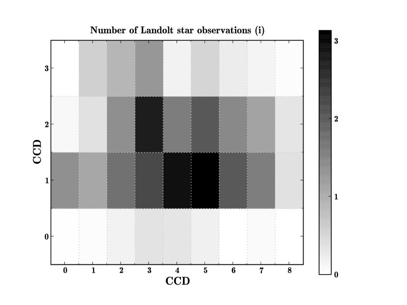
Landolt fields are observed almost each potentially photometric night. The flux of the Landolt stars is measured using the aperture photometry algorithm described in section 4. On average, between 2 and 3 stars are observed each night, in each band, on each central CCD (figure 13). On the other hand, less than 0.5 Landolt star per night are observed on the CCDs which are on the sides of the focal plane. The Landolt star observations allow us to determine the zero-points of each night, in each band, along with additional (nuisance) parameters, such as the coefficients describing the Landolt to MegaCam transformations and the mean airmass coefficients.

Figure 13: Average number of Landolt star observations per CCD, in the $i_{M}$-band. CCD number 0 is top left, while CCD number 35 bottom right. Two to three stars per night and per band are observed on the central CCDs. On the other hand, often less than 0.5 (and even less than 0.1 for CCDs 27 to 35) star are observed on the CCDs located on the side of the focal plane. Hence, each CCD cannot be calibrated independently, and we have to rely on the uniformity maps to propagate the calibration to the entire focal plane.

Due to the significant differences between the Landolt Johnson-Kron-Cousins-$UBVRI$ and MegaCam $g_{M},r_{M},i_{M},z_{M}$ filter-sets, the Landolt-to-MegaCam color transformations were found to be large and even non-linear. We model them using piecewise-linear functions of the form:

$${C}({\rm color};\alpha,\beta)=\begin{cases}\ \alpha\times{\rm color},\ \ \ \ \text{if ${\rm color}<{\rm color}_{break}$}\\ \ \alpha\times{\rm color}_{break}+\beta\times\Bigl{(}{\rm color}-{\rm color}_{break}\Bigr{)},\\ \ \ \ \ \ \ \ \ \ \ \ \ \ \ \ \ \ \ \ \ \ \ \ \ \ \ \ \ \ \ \ \ \ \ \ \ \ \ \ \ {\text{otherwise}}\\ \end{cases}$$

where ${\rm color}$ is a Landolt color. The equation above has three unknown parameters: 2 slopes, $\alpha$ and $\beta$, and a “color break” marking the transition between the two slopes. The slopes $\alpha$ and $\beta$ are fitted along with the zero-points. The parameter ${\rm color}_{break}$ is adjusted by studying the fit residuals, and fixed. We have found that the sensitivity of the zero points to the break position is small: in all bands they vary by less than 0.0015 mag if the break varies by 0.1 mag. As discussed above, if we choose a fundamental standard whose colors are similar to the Landolt star colors, the impact of the break position will be even smaller than 0.001 mag.

Since the MegaCam passbands are not uniform, there are, in practice as many photometric systems as there are locations on the focal plane. The density of Landolt stars in the calibration fields does not allow us to calibrate independently each location, and we must rely on the grid maps to propagate the calibration to the whole focal plane. To establish the calibration equations, let’s first assume that the Landolt stars are all observed at the reference location, ${\mathbf{x}}_{0}$. The relations between the MegaCam instrumental “hat magnitudes” (corrected for “gray” non-uniformities) as defined in §6 and the magnitudes reported by Landolt ($UBVRI$) can be parametrized as:

$$\hat{g}_{ADU|{\mathbf{x}}_{0}} = V -k_{g}(X-1) +C(B-V;\alpha_{g},\beta_{g}) +ZP_{g}$$

$$\hat{r}_{ADU|{\mathbf{x}}_{0}} = R -k_{r}(X-1) +C(V-R;\alpha_{r},\beta_{r}) +ZP_{r}$$

$$\hat{i}_{ADU|{\mathbf{x}}_{0}} = I -k_{i}(X-1) +C(R-I;\alpha_{i},\beta_{i}) +ZP_{i}$$

$$\hat{z}_{ADU|{\mathbf{x}}_{0}} = I -k_{z}(X-1) +C(R-I;\alpha_{z},\beta_{z}) +ZP_{z}$$

$X$ is the airmass of the observation, $k_{u},\ldots k_{z}$ are the airmass coefficients and $ZP_{u},\ldots ZP_{z}$ the zero-points. The free parameters of the calibration relations above are the five airmass terms $k_{ugriz}$, the ten color transformations slopes $\alpha_{ugriz}$ and $\beta_{ugriz}$ and about 1600 zero points —one zero-point per night and per band. All these parameters are fit simultaneously on the whole calibration dataset.

The airmass range of the calibration data taken each night is extremely variable and does not allow one to fit an airmass coefficient per night and per band. For this reason, we have chosen to fit one global airmass coefficient per band. This has no consequence on the tertiary magnitudes which are built by averaging the data coming from many different epochs.

Quite often, second order terms of the form $k^{\prime}\times(X-1)\times{\rm color}$ enter the airmass parametrization and are neglected here. This will be discussed in more detail in §12. We have estimated the magnitude of these contributions using the passband models discussed in §7 and synthetic photometry and found them to be extremely small ($<0.001$ mag).

In reality, the Landolt stars are not observed at the focal plane reference location, but at many random locations. We therefore rely on the grid transformations determined in §6 in order to relate the instrumental magnitudes of the Landolt stars at any position with the same magnitudes at the reference position. The calibration equations actually implemented in the zero-point fit are therefore a little more complex:

$$\hat{g}_{ADU|{\mathbf{x}}} = \delta k_{ggr}({\mathbf{x}})\ \Bigl{(}(g-r)_{|{\mathbf{x}}_{0}}-(g-r)_{grid}\Bigr{)}+V -k_{g}(X-1) +$$

$$C(B-V;\alpha_{g},\beta_{g})+ZP_{g}$$

$$\ldots$$

$$\hat{z}_{ADU|{\mathbf{x}}} = \delta k_{ziz}({\mathbf{x}})\ \Bigl{(}(i-z)_{|{\mathbf{x}}_{0}}-(i-z)_{grid}\Bigr{)}+I -k_{z}(X-1) +$$

$$C(R-I;\alpha_{z},\beta_{z})+ZP_{z}$$

These equations imply that the MegaCam colors of the Landolt stars, measured at the reference location: $(g-r)_{|{\mathbf{x}}_{0}}$, …$(i-z)_{|{\mathbf{x}}_{0}}$ must be determined in the course of the calibration fit. They are determined iteratively from the MegaCam observations of the Landolt stars: in a first pass, we ignore the color grid corrections and obtain a first approximation of the MegaCam colors of the Landolt stars. These colors are then injected into the fit, and we iterate.

The fact that the grid reference colors appear explicitly in the calibration equations may seem a little odd. As mentioned above, these colors are internal quantities, and should not impact the calibration. Indeed, it can be verified that changing the grid reference colors and changing the $\delta zp({\mathbf{x}})$ maps entering in the definition of the hat magnitudes accordingly has no impact on the value of the zero points.

Finally, a few words must be said about the uncertainty model. One must recall that the Landolt stars do not form an exact one-parameter sequence, and cannot be perfectly indexed by one color only. In practice, the Landolt-MegaCam color-color diagrams are affected by an intrinsic star-to-star dispersion partly of astrophysical origin, of about 1% in the $g_{M}r_{M}i_{M}$-bands and 2% in the $z_{M}$-band. The dispersion of the fit residuals is dominated by this star-to-star dispersion and not by the star measurement uncertainties (closer to 0.1%). Since each star is measured several times, this means that the error model has a very specific structure which must be modeled. The star-to-star dispersion, in each band, is estimated from the fit residuals. The correlations between the same band contributions of each star are accounted for by fitting one additional parameter per star and per band, $\delta{\rm mag}$, this parameter being constrained by adding terms in the $\chi^{2}$ of the form $\left(\delta{\rm mag}/\sigma_{star-to-star}\right)^{2}$.

8.3 Results

Table 6: Landolt to MegaCam color transformation slopes and airmass correction terms.

band	Landolt	color	$\alpha$	$\beta$	$k$	$k_{Elixir}$ a
	color index	break
$g_{M}$	$B-V$	$+0.45$	$+0.4957\pm 0.0153$	$+0.4583\pm 0.0026$	$-0.1830\pm 0.0017$	$-0.15$
$r_{M}$	$V-R$	$+0.65$	$+0.1654\pm 0.0049$	$+0.2079\pm 0.0248$	$-0.1346\pm 0.0017$	$-0.10$
$i_{M}$	$R-I$	$+0.40$	$+0.2069\pm 0.0093$	$+0.1702\pm 0.0056$	$-0.0467\pm 0.0017$	$-0.04$
$z_{M}$	$R-I$	$+0.35$	$-0.1949\pm 0.0301$	$-0.4420\pm 0.0133$	$-0.0585\pm 0.0034$	$-0.03$

• canonical airmass coefficients reported by the Elixir pipeline in the image headers.

(a) $g_{M}-V\ vs.\ B-V$

(b) $r_{M}-R\ vs.\ V-R$

(c) $i_{M}-I\ vs.\ R-I$

(d) $z_{M}-I\ vs.\ R-I$

Figure 14: Upper panels: color-color plots considered in the $g_{M}$, $r_{M}$, $i_{M}$ and $z_{M}$ zero-point fits. The black points correspond to individual Landolt star measurements. The red points are the average of the calibrated measurements of a same star. The color-color transformations are modeled as piecewise-linear functions, with breaks at $B-V=+0.45$, $V-R=+0.65$, $R-I=+0.40$ and $R-I=+0.35$ in the $g_{M}$, $r_{M}$, $i_{M}$ and $z_{M}$ bands respectively. Lower panels: color-color plots residuals (average of each Landolt star’s calibrated measurements only).

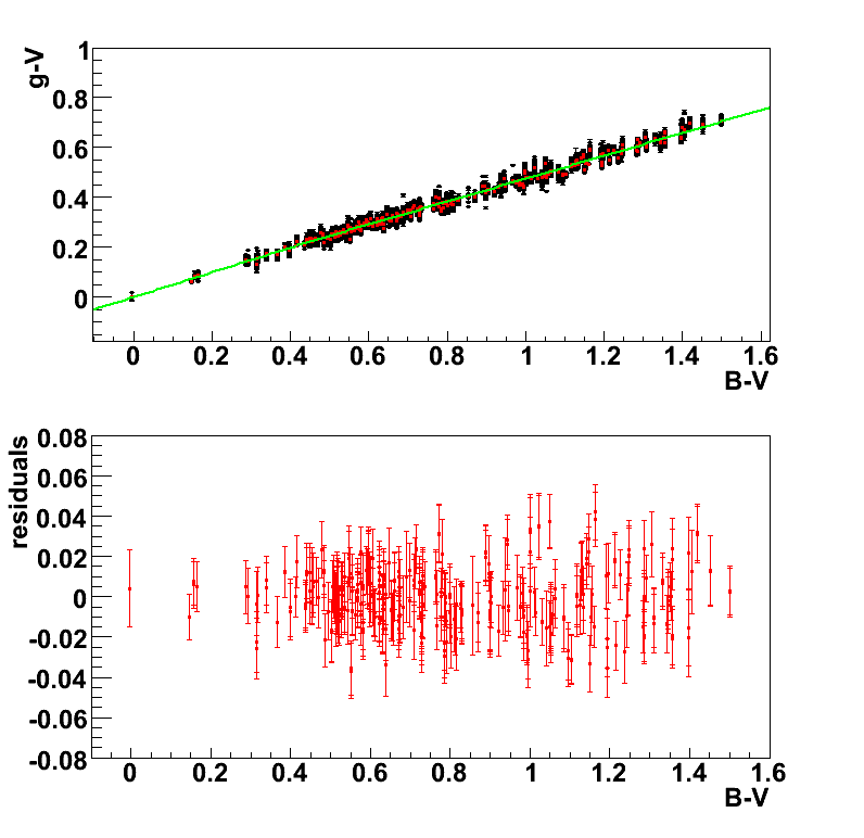
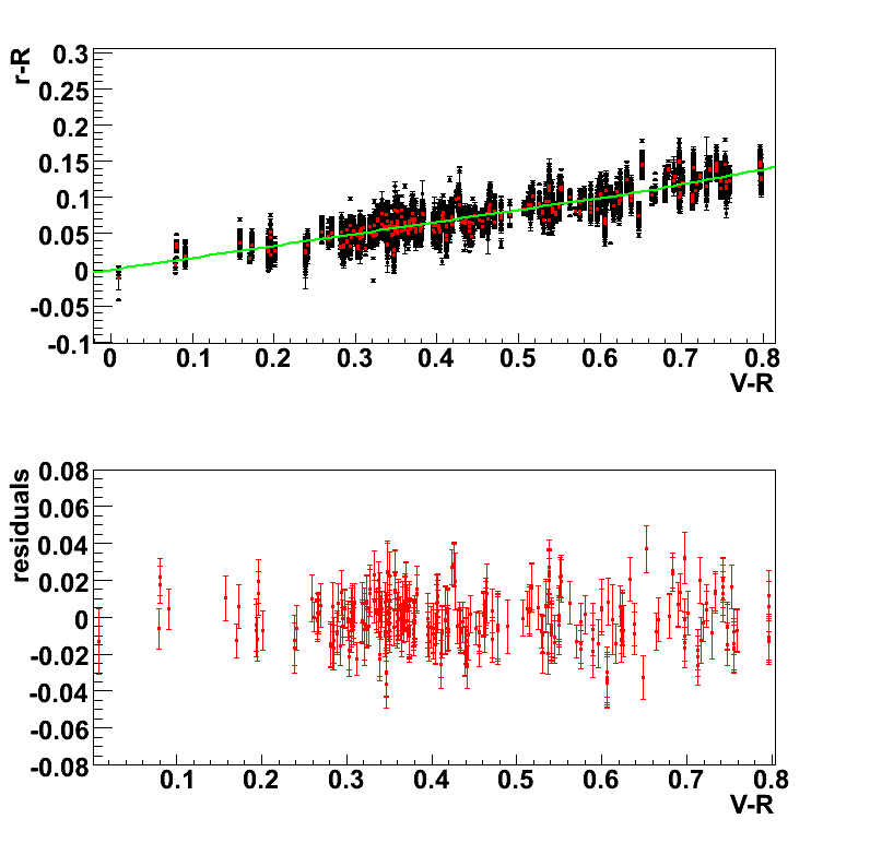
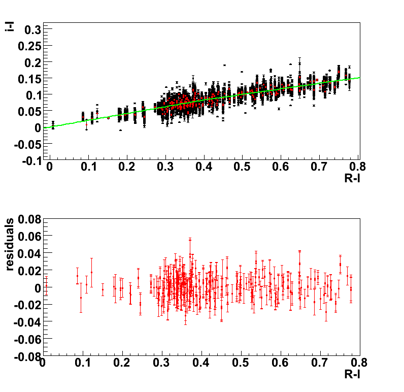
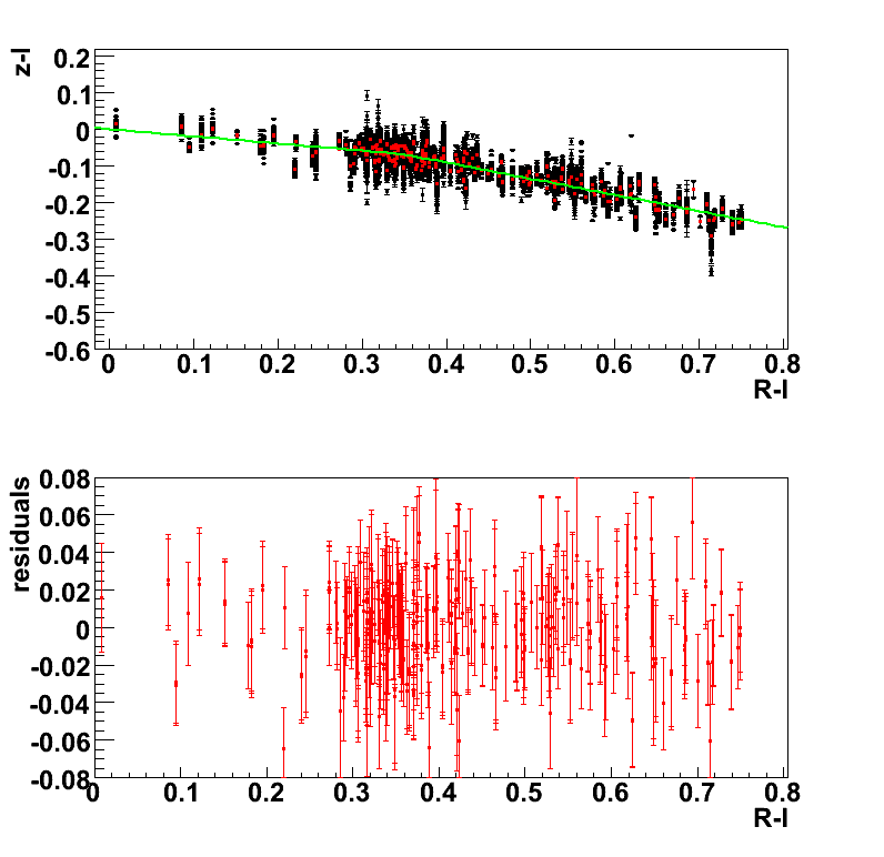
Figure 14 presents the color-color diagrams considered in the zero-point fit described above. The parameters of the Landolt-to-MegaCam color transformations are summarized in table 6. These slopes are measured with precisions of about 1% on average, this error budget being dominated by the star-to-star dispersion.

(a) $g_{M}$

(b) $r_{M}$

(c) $i_{M}$

(d) $z_{M}$

Figure 15: $g_{M}$, $r_{M}$, $i_{M}$ and $z_{M}$ zero-point as a function of time. The zero-point evolution is classically due to dust accumulating in the optical path and the natural degradation of the mirror coating over time. We also indicate the main events (recoating, labeled “[R]”, and washings “[W]”) which affected the primary mirror during the three first years of the survey. The significant improvement observed around +200 days is due a mirror recoating (August 15th, 2003). The effect of two additional mirror cleanings, which took place on April 14th, 2004 and January 26th, 2005 are also clearly visible. The full MegaCam / MegaPrime history log is available at http://www.cfht.hawaii.edu/Instruments/Imaging/MegaPrime/megaprimehistory.html.

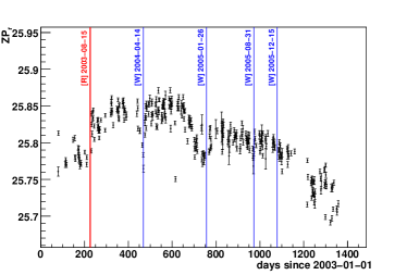
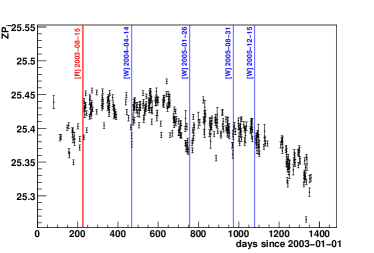
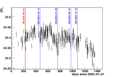
The airmass coefficients are summarized in table 6. As can be seen, they do differ from the mean coefficients reported by Elixir, and these differences induce sizeable differences on the calibrated magnitudes.

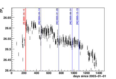
Figure 15 presents the variation of the $g_{M},r_{M},i_{M}$ and $z_{M}$ zero-points as a function of time. The effect of dust accumulating on the optical path is clearly visible. The recoveries observed at various points of the survey can be explained with the full MegaCam / MegaPrime history log. The spectacular improvement observed at the beginning of the survey is due to the recoating of the mirror (August 15th, 2003). Two additional significant improvements were due to mirror cleanings (April 14th, 2004 and January 26th, 2005). Note that an additional mirror recoating took place on August, 2007, during the fourth year of the survey. It allowed one to recover the efficiency levels observed at the beginning of the survey.

The zero-point uncertainties determined at this stage are of about 0.007, 0.003, 0.004 and 0.011 mag in the $g_{M},r_{M},i_{M}$- and $z_{M}$-bands respectively. These uncertainties, are dominated by the uncertainties on the color transformation parameters discussed above. Indeed the average Landolt star colors are very far from zero: $B-V\sim 0.77$, $V-R\sim 0.46$ and $R-I\sim 0.42$. Since the color transformations are global, this also means that the zero-points in a given band are correlated. If we remove the color transformation contributions, the intrinsic zero-point uncertainties are of about 0.003 mag in the $g_{M},r_{M},i_{M}$-bands and 0.005 mag in $z_{M}$.

We will see in the next sections that the impact of the zero-point uncertainties on the flux interpretation of the tertiary standard actually depends on the colors of the fundamental standard used to interpret the fluxes. If we choose a standard such as Vega, the color transformation uncertainties will dominate. If we choose a star whose colors are closer to the average Landolt star colors, the zero-point contributions to the calibrated flux error budget will be close to the intrinsic uncertainties.

9 MegaCam Magnitudes

We are now ready to define the MegaCam magnitude system. As discussed in the introduction of this paper, a requirement of the SNLS calibration is that the MegaCam magnitudes must be easily interpreted as physical fluxes. This requires that the MegaCam magnitudes be defined as natural magnitudes, i.e. their definition should not integrate any term depending on each star’s color.

9.1 Uniform Magnitudes

First, let’s assume that the MegaCam passbands are spatially uniform. Or equivalently, that all our tertiary standards are observed at the focal plane reference location. In this case, the definition of the MegaCam magnitudes is:

$$g_{|{\mathbf{x}}_{0}} \equiv \hat{g}_{ADU|{\mathbf{x}}_{0}}+ZP_{g}$$

$$\ldots$$

$$z_{|{\mathbf{x}}_{0}} \equiv \hat{z}_{ADU|{\mathbf{x}}_{0}}+ZP_{z}$$

In reality, the tertiary standards are observed at various reference locations. But since we know how the hat magnitudes transform all over the focal plane, we can define the MegaCam magnitudes as:

$$g_{|{\mathbf{x}}_{0}} \equiv \hat{g}_{ADU|{\mathbf{x}}}-\delta k_{ggr}({\mathbf{x}})\times\Bigl{[}(g-r)_{|{\mathbf{x}}_{0}}-(g-r)_{grid}\Bigr{]}+ZP_{g}$$

$$\ldots$$

$$z_{|{\mathbf{x}}_{0}} \equiv \hat{z}_{ADU|{\mathbf{x}}}-\delta k_{ziz}({\mathbf{x}})\times\Bigl{[}(i-z)_{|{\mathbf{x}}_{0}}-(i-z)_{grid}\Bigr{]}+ZP_{z}$$ (6)

With this definition, the calibrated magnitudes do not depend on the focal plane position where the stars have been observed. We call them Uniform Magnitudes. These are typically the kind of magnitudes we would like to report to the end users, since they hide the complexity of the MegaCam imager to the external user. However, the Uniform Magnitudes are not natural magnitudes: indeed, they include a color term in their definition.

9.2 Local Natural Magnitudes

The definition above tells us how to define the MegaCam natural magnitudes. They must incorporate the grid color corrections. We define these magnitudes as:

$$g_{|{\mathbf{x}}} \equiv {g}_{|{\mathbf{x}}_{0}}+\delta k_{ggr}({\mathbf{x}})\times\Bigl{[}(g-r)_{|{\mathbf{x}}_{0}}-(g-r)_{ref}\Bigr{]}$$

$$\ldots$$

$$z_{|{\mathbf{x}}} \equiv {z}_{|{\mathbf{x}}_{0}}+\delta k_{ziz}({\mathbf{x}})\times\Bigl{[}(i-z)_{|{\mathbf{x}}_{0}}-(i-z)_{ref}\Bigr{]}$$ (7)

where $g_{|{\mathbf{x}}_{0}}$ …$z_{|{\mathbf{x}}_{0}}$ are the magnitudes defined above, and $(g-r)_{ref}$ …$(i-z)_{ref}$ arbitrary color zero points. With this definition, the relation between the calibrated magnitudes and the instrumental magnitudes is:

$$g_{|{\mathbf{x}}} = \hat{g}_{ADU|{\mathbf{x}}}+ZP_{g}-\delta k_{ggr}({\mathbf{x}})\times\Bigl{[}(g-r)_{ref}-(g-r)_{grid}\Bigr{]}$$

$$\ldots$$

$$z_{|{\mathbf{x}}} = \hat{z}_{ADU|{\mathbf{x}}}+ZP_{z}-\delta k_{ziz}({\mathbf{x}})\times\Bigl{[}(i-z)_{ref}-(i-z)_{grid}\Bigr{]}$$ (8)

As we can see, the $g_{|{\mathbf{x}}}$, …$z_{|{\mathbf{x}}}$ form a natural magnitude system. We call them Local Natural Magnitudes. On the other hand, the definition of these magnitudes explicitly depends on where each star was observed on the focal plane.

Once again, it is easy to verify that the calibrated magnitudes do not depend on the choice of the grid reference colors, since the quantities $\hat{m}_{ADU|{\mathbf{x}}}+\delta k({\mathbf{x}})\times({\rm color}_{grid})$ are themselves independent of those reference colors. We also have introduced another set of reference colors: $(g-r)_{ref},\ldots(i-z)_{ref}$. These colors have the same status as the grid reference colors: they have been introduced to make explicit that there is some degree of arbitrariness in the Local Magnitude definition. In practice, it is useful to take these colors equal the colors of the fundamental standard at the center of the focal plane:

$$(g-r)_{ref} = (g-r)_{|{\mathbf{x}}_{0}}^{ref}$$

$$(r-i)_{ref} = (r-i)_{|{\mathbf{x}}_{0}}^{ref}$$

$$(i-z)_{ref} = (i-z)_{|{\mathbf{x}}_{0}}^{ref}$$

10 Flux Interpretation of the MegaCam Magnitudes

Now that we have defined a system of natural magnitudes, we still have to explicit the magnitude to flux conversion. To do this, we rely on a “fundamental spectrophotometric standard”, i.e. a star of known SED, $S_{ref}(\lambda)$ and known MegaCam magnitudes in the system defined above. The calibrated broadband flux, $F_{|{\mathbf{x}}}$ of an object of magnitude $m_{|{\mathbf{x}}}$ is then:

$$\text{F}_{|{\mathbf{x}}}=10^{-0.4\ \left(m_{|{\mathbf{x}}}-m_{ref}\right)}\times\int S_{ref}(\lambda)T(\lambda;{\mathbf{x}})d\lambda$$ (9)

where $T(\lambda;{\mathbf{x}})$ is the effective passband of the imager at location ${\mathbf{x}}$ on the focal plane.

Systematic uncertainties affect this mapping function. First, the MegaCam passbands are not known perfectly. Furthermore, the SED of the fundamental standard is not perfectly measured. Finally, the MegaCam magnitudes of the fundamental standard, in the system defined in the previous section are not known perfectly. At best, the fundamental standard is directly observed with the survey telescope, and the measurement uncertainties must be taken into account. Most often, the fundamental standard is too bright to be directly observed, and its magnitudes must be inferred in some way, introducing additional uncertainties.

It must also be noted that the quantities relevant for the cosmology studies are not exactly physical fluxes, but rather the ratio of physical fluxes, measured in different passbands. In other words, the cosmological measurements are completely insensitive to any change of the absolute flux scale. For this reason, we report the uncertainties of the fluxes and magnitudes relative to a reference band, namely the Landolt $V$-band. In particular, the relevant uncertainties are those affecting (1) the ratios $\int S_{ref}(\lambda)T(\lambda;{\mathbf{x}})d\lambda/\int S_{ref}(\lambda)V(\lambda)d\lambda$ and (2) the colors $g_{ref}-V$, $r_{ref}-V$, $i_{ref}-V$ and $z_{ref}-V$.

10.1 Selecting a Fundamental Standard

No spectrophotometric standard usable as a fundamental standard has reliable magnitudes established from MegaCam observations. Such a program is underway, but has not been completed yet. The MegaCam magnitudes of the fundamental standard must therefore be infered from its Landolt magnitudes, using the Landolt to MegaCam color transformations. For example, if the Landolt colors of the star are bluer than the color break:

$$g_{|{\mathbf{x}}_{0}}^{ref} = V^{ref}+\alpha_{g}\times(B-V)^{ref}+\Delta g^{ref}_{|{\mathbf{x}}_{0}}$$

$$\ldots$$

$$z_{|{\mathbf{x}}_{0}}^{ref} = I^{ref}+\alpha_{z}\times(R-I)^{ref}+\Delta z^{ref}_{|{\mathbf{x}}_{0}}$$ (10)

where the quantities $\Delta m^{ref}_{|{\mathbf{x}}_{0}}$ account for the fact that the fundamental standard departs slightly from the Landolt-to-MegaCam color-color law. The uncertainties on the MegaCam magnitudes of the fundamental standard account directly as systematic errors on the calibrated fluxes. The $\Delta m^{ref}_{|{\mathbf{x}}_{0}}$ offsets can be as large as one percent, given the standard deviation of the residuals to the Landolt-to-MegaCam color laws. Hence, they must be evaluated, using synthetic photometry. Furthermore, we point out that the uncertainty on the Landolt-to-MegaCam color transformations also affect the estimates of $g_{|{\mathbf{x}}_{0}}$, …$z_{|{\mathbf{x}}_{0}}$. Our concern in this section, is therefore to choose a fundamental standard, which would allow us to minimize this error budget.

A standard choice is the star $\alpha$-Lyræ, also called Vega. Vega is one of the six A0V stars that define the zero-points of the historical Johnson & Morgan (1951, 1953) UBV system. The Landolt magnitudes of this star being all close to zero (although not exactly zero), the Landolt system is often (improperly) referred to as a “Vega based system” and the SED of Vega is generally used to convert the Landolt magnitudes into fluxes. This was the approach used in Astier et al. (2006). The “canonical” magnitudes of Vega reported, for example in Fukugita et al. (1996) were used to twist the SED of Vega measured by Bohlin & Gilliland (2004b) and to get an approximation of the SED of the hypothetical fundamental standard of the Landolt system.

However, a close study of the systematic error budget shows that Vega is not a wise choice if we seek a 1% precision or better on the calibrated fluxes. First, Landolt did not actually observe Vega directly while building his catalogs due to its brightness. An estimate of the Landolt Vega $U-B$ and $B-V$ colors can be obtained by propagating the initial measurements of Johnson & Morgan (1951) through the color transformations cited by Landolt (1973, 1983, 1992b). The $R-I$ color index can traced back from the original Cousins (1978) papers. However, values of $R-I$ that differ by about 0.05 mag are cited in Taylor (1986); Fukugita et al. (1996). Furthermore, no measurement of the $V-R$ color index could be found in the literature. In any case, it is not possible to guarantee a precision of 0.01 mag on the Vega magnitudes reconstructed in such a way.

Another problem with Vega, is that it is significantly bluer than the average Landolt star ($B-V\sim 0.77$) and the average tertiary standards. As discussed in §8, there are large uncertainties associated with the modeling of the Landolt-to-MegaCam color transformations. In particular, given the low number of blue Landolt stars, it is nearly impossible to tell anything about the linearity of the color transformations in the bluer parts of the color-color diagrams. Furthermore, as noted in §8, the blue side of the Landolt-to-MegaCam transformations (the $\alpha$ parameters) are determined with a precision not better than 1.5% in $g$ and $3\%$ in $z$. This induces an additional uncertainty of about 1% on the MegaCam colors of Vega infered with equation 10. This problem disappears if we use, as a fundamental standard, a star of colors close to the average color of the Landolt stars, and if possible, a star directly observed by Landolt.

Few Landolt stars have measured spectral energy distributions, covering the wavelength-range $3000\AA\ -11000\AA$ covered by MegaCam. The HST community has put considerable effort into building a database of high-quality spectrophotometric standards —the so-called CALSPEC database (Bohlin, 2000a). An absolute flux scale was defined, based on NLTE models of three pure hydrogen white-dwarfs: G191-B2B, GD 153 and GD 71. The SEDs of several key standards such as Vega and BD +17 4708 have been re-observed and re-calibrated with the Space Telescope Imaging Spectrograph (STIS) and the Near Infrared Camera and Multi-Object Spectrometer (NICMOS) instruments (Bohlin, 2000b; Bohlin & Gilliland, 2004b; Bohlin, 2007). More recently, Landolt & Uomoto (2007, hereafter LU07) published magnitudes of some of the CALSPEC HST spectrophotometric standards. Combining these two sources, we found that six stars have simultaneously known Landolt magnitudes and known SEDs, published by the CALSPEC project and measured exclusively with the HST STIS and NICMOS instruments: AGK +81 266, BD +17 4708, G 191-B2B, GD 71, GRW 705824 and LDS 749B. Most of these objects are very blue stars, except BD +17 4708, whose colors are close to the average Landolt colors.

We have therefore selected BD +17 4708 as a fundamental standard. This F8-type star has been chosen as a fundamental standard for many photometric systems, notably that of the Sloan Digital Sky Survey (SDSS) (Fukugita et al., 1996; Smith et al., 2002; Gunn et al., 1998, 2006; Ivezić et al., 2007) and consequently has been studied by many groups, which have derived estimates of its extinction, effective temperature, metallicity and surface gravity (see Ramírez et al., 2006, and references therein). Bohlin & Gilliland (2004a) have measured the absolute spectral energy distribution of BD +17 4708 in the wavelength range $1700\ \AA<\lambda<10000\ \AA$, with an accuracy of less than 0.5% in the transfer of the flux calibration of the three white dwarfs primary standards, and an accuracy of the relative flux distribution of about 2%.

On the other hand, it has been pointed out that BD +17 4708 may be a binary system, with a faint late-M companion of mass $\sim 0.15M_{\odot}$ revolving around the main star in about 220 days (Latham et al., 1988; Ramírez et al., 2006). Furthermore, with a $V$-band magnitude of 9.464, BD +17 4708 is a little bright to be observed directly with MegaCam with a good accuracy. The indirect determination of its MegaCam magnitudes is presented in the next section.

In addition to BD +17 4708, LU07 present magnitudes for the fundamental CALSPEC white dwarf calibrators. We also considered using these stars, but the fact that they are even bluer than Vega exacerbates the extrapolation problem when calculating their MegaCam magnitudes. Furthermore, there is some evidence that a similar problem affects the Landolt magnitudes themselves. As noted earlier, the original Landolt telescope/detector system no longer exists, so the magnitudes tabulated in LU07 have been transformed from some natural system to the Landolt (1992b) system using a similar method as that described in 9.1. These transformations were calculated using “typical” Landolt stars, which are much redder than the white dwarfs. Therefore, these transformations may not be accurate for the very blue white dwarfs, especially in $B$ and $U$ where the absence of a Balmer break makes the SEDs very different.

Without knowing the exact Landolt catalog system passbands we have no way of precisely calculating the amount of bias present or correcting for it, but we can check for the plausibility of this issue by simulating a similar set of observations and reduction procedures as actually used by LU07. We start with an assumed model for the Landolt catalog passbands Bessell (1990) and use the natural system passbands given in LU07, folding in mirror reflectivity and photomultiplier response, then carry out synthetic photometry using a library of SEDs Pickles (1998) in both systems. We then calculate multi-step linear transformations following the prescription of Landolt (1992b) using the redder stars and compare the transformed magnitudes of the CALSPEC WDs to the actual synthetic magnitudes in the natural system. We find that the transformations are biased at the 1-2% level, particularly in $B$ where the LU07 $B$ filter has a “notch” near the peak transmission. The exact amount of bias is sensitive to the assumed Landolt catalog filters, but its existence is not. We conclude that there is reason to be cautious when using the WDs for photometric calibration. Note that these concerns have no effect on the CALSPEC spectroscopic calibration.

10.2 The MegaCam Magnitudes of BD +17 4708

At first order, the MegaCam magnitudes of BD +17 4708 can be derived from the magnitudes and colors reported by Landolt, and the Landolt-to-MegaCam color transformations determined in §8 (see equation 10). In table 7, we report the $g_{M}-V$, $r_{M}-V$, $i_{M}-V$ and $z_{M}-V$ colors of BD +17 4708. The uncertainties quoted by Landolt are propagated, assuming that the magnitudes and colors $V$, $B-V$, $V-R$ and $R-I$ reported by Landolt are essentially independent. Note that the $i_{M}-V$ and $z_{M}-V$ are strongly correlated, with a correlation coefficient of 0.96. The statistical uncertainties affecting the Landolt-to-MegaCam color transformations do also affect the MegaCam colors reported in table 7. However, we will see in §11 that the impact of the color transformations on the calibrated tertiary fluxes is actually much smaller. As a consequence, we do not include them in the final uncertainty budget listed in table 7.

The determination of the offsets $\Delta g_{|{\mathbf{x}}_{0}}^{ref}$ …$\Delta z_{|{\mathbf{x}}_{0}}^{ref}$ defined in equation 10 is a little more complex. These quantities account for how the BD +17 4708 magnitudes differ, on average, from those of the Landolt stars whose colors are close to BD +17 4708. To estimate them, we will rely on (1) estimates of the extinction, temperature, metallicity and surface gravity of BD +17 4708, (2) rough estimates of the same quantities for Landolt stars of colors similar to those of BD +17 4708 and (3) the Phoenix library of synthetic star SED models (Hauschildt et al., 1997; Baron & Hauschildt, 1998; Hauschildt & Baron, 1999, and references therein).

The extinction, temperature, surface gravity and metallicity of BD +17 4708 are estimated in Ramírez et al. (2006): $E(B-V)\simeq 0.010\pm 0.003$, $T_{eff}\simeq 6141\pm 50K$, $\log g=3.87\pm 0.08$ and $[{\rm M/H}]=-1.74\pm 0.09$. (Ramírez et al., 2006) also gives rough estimates of the type (late-M), mass ($\sim 0.15M_{\odot}$) and effective temperature ($\sim 3000K$) of its faint companion.

On the other hand, not much is known about the Landolt stars. We assume them to be nearby disk stars. Their mean metallicity may be derived from Ramírez et al. (2007): $-0.5<[{\rm M/H}]<-0.3$, substantially higher than the metallicity of BD +17 4708. Landolt stars of colors similar to those of BD +17 4708 have an effective temperature $T_{eff}\sim 6200K$ and a surface gravity $\log g\sim 4.3$ (Allen, 1976). In what follows, we estimate the magnitude offsets induced by (1) the fact that BD +17 4708 is a likely binary system (2) the metallicity differences between BD +17 4708 and the mean Landolt star (3) the surface gravity differences and (4) the extinction differences.

Binarity

We can estimate the impact of the likely faint companion with synthetic photometry. We select the Phoenix stellar models whose parameters are as close as possible to those of BD +17 4708 and its companion, respectively $T_{eff}=6000K$, $\log g=3.5$, $[M/H]=-2$ and $T_{eff}=3000K$, $\log g=4.5$ and $[M/H]=-2$ (Ramírez et al., 2006). The impact on the calibration is given by the difference of residuals to the Landolt-to-MegaCam color transformation, with and without the contribution of the faint companion. We obtain (in the sense with companion minus without companion):

$$\Delta g\simeq+0.001$$

$$\Delta r\simeq+0.004$$

$$\Delta i\simeq-0.002$$

$$\Delta z\simeq-0.015$$ (11)

There is a large uncertainty, of about 50% on those numbers. We account for them as additional systematic uncertainties, as we do not known the fraction of Landolt stars that are also in binary systems.

Metallicity

As noted above the metallicity of BD +17 4708 is significantly lower than that of Landolt stars of similar colors. The impact of this difference was estimated by computing the offsets between the MegaCam synthetic magnitudes of GAIA / Phoenix stars of metallicities and colors close to that of BD +17 4708, and the synthetic magnitudes of Phoenix SEDs of similar colors but metallicity close to that of Landolt stars. We obtained the following offsets (in the sense BD +17 4708 mag minus Landolt mag):

$$\Delta g=+0.007\pm 0.002$$

$$\Delta r=+0.003\pm 0.001$$

$$\Delta i=+0.002\pm 0.001$$

$$\Delta z=-0.009\pm 0.001$$ (12)

These offsets are applied to the first order estimates of the magnitudes of BD +17 4708.

Surface Gravity

The impact of the surface gravity differences between the Landolt stars and BD +17 4708 can be evaluated in a similar fashion. We find that the corrections are smaller than 0.001 mag in all bands except in $z_{M}$ (in the sense BD +17 4708 mag minus Landolt mag):

$$\Delta z=-0.001\pm 0.003$$ (13)

We apply this offset to the BD +17 4708 magnitude estimates, and retain a systematic uncertainty of 0.003 mag in the systematic error budget.

Extinction

The mean reddening affecting the Landolt stars is poorly known. It can be constrained by the locus of the Landolt stars, in the $V-R$ vs. $R-I$ color-color diagram. Indeed, the $V-R$ and $R-I$ colors of the Landolt stars are very well correlated in the color region of BD +17 4708. More precisely, the quantity $\Delta_{VRI}=(R-I)-0.7(V-R)$, computed in the same color region, has an RMS of 0.019 and an average value of $0.995\pm 0.002$. For BD +17 4708, $\Delta_{VRI}=0.111$. This quantity can be related to unmeasured quantities such as the reddening using synthetic photometry:

$$\Delta_{VRI}^{BD\leavevmode\nobreak\ +17\leavevmode\nobreak\ 4708}-\Delta_{VRI}^{Landolt} = \frac{\partial\Delta_{VRI}}{\partial E(B-V)}\ \delta E(B-V)+$$

$$\frac{\partial\Delta_{VRI}}{\partial[M/H]}\ \delta[M/H]+$$

$$\frac{\partial\Delta_{VRI}}{\partial\log g}\ \delta\log g$$

Using the Phoenix models, we find that the derivatives of $\Delta_{VRI}$ w.r.t. the extinction and metallicity in the color region of BD +17 4708 to be, respectively: $0.22$, $0.02$, the effect of the surface gravity being essentially negligible in this color range. This can be translated into a constraint on the extinction difference between BD +17 4708 and the Landolt stars of similar colors:

$$\Delta E(B-V)=E(B-V)(BD\ +17)-E(B-V)({\rm Landolt})\simeq 0.045$$

Again, using synthetic photometry and the Cardelli et al. (1989) law, this can be translated into calibration offsets:

$$\Delta g_{M} =-0.01\times\Delta E(B-V) =-0.0005$$

$$\Delta r_{M} =+0.02\times\Delta E(B-V) =+0.0009$$

$$\Delta i_{M} =+0.01\times\Delta E(B-V) =+0.0005$$

$$\Delta z_{M} =-0.19\times\Delta E(B-V) =-0.0085$$ (14)

The effect of the reddening differences between BD +17 4708 and the Landolt stars impacts essentially the $z_{M}$-band magnitudes, because this band requires an extrapolation from $I$ to $z_{M}$. We will consider these offsets as additional systematic uncertainties.

To summarize: we have derived MegaCam Natural colors $g-V$, $r-V$, $i-V$ and $z-V$ for BD +17 4708, relying on the Landolt-to-MegaCam color transformations, and on synthetic photometry computed from the Phoenix / GAIA spectral library. The results along with their uncertainties are summarized in table 7. The Landolt magnitudes of BD +17 4708, as well as our estimates of the BD +17 4708 MegaCam magnitudes are all correlated. The full covariance matrix, ${\mathbf{V}}_{BD\leavevmode\nobreak\ +17\leavevmode\nobreak\ 4708}$, reported in table 19 (appendix D) is the sum of two $9\times 9$ components:

$${\mathbf{V}}_{BD\leavevmode\nobreak\ +17\leavevmode\nobreak\ 4708}={\mathbf{V}}_{Landolt}+{\mathbf{V}}_{\Delta m}$$

${\mathbf{V}}_{\Delta m}$ contains the uncertainties on the deviations to the linear Landolt-to-MegaCam color corrections derived in this section and assumed to be independent. ${\mathbf{V}}_{Landolt}$ accounts for the Landolt uncertainties on the $g-V$, $r-V$, $i-V$, $z-V$, $U-V$, $B-V$, $R-V$ and $I-V$-colors. Note that since Landolt & Uomoto (2007) do not discuss the correlations between their measurement uncertainties, we had to make an assumption on their error budget: we have chosen to assume that their $V$, $U-B$, $B-V$, $V-R$, $R-I$ and $V-I$ measurements are essentially independent. This is equivalent to assuming that the individual magnitudes measurements are all affected by an overall “gray” uncertainty, that correlate them positively. This “gray” uncertainty is reflected in the higher $V$-band uncertainty reported by Landolt & Uomoto (2007). The uncertainties on the MegaCam $X-V$ colors are obtained by propagating the Landolt errors using equation 10.

To be complete, we should also add the contribution of the uncertainties that affect the Landolt-to-MegaCam transformation coefficients themselves. However, as will be discussed later, this contribution is itself strongly correlated with the zero-point uncertainties, hence with the tertiary star magnitudes. Since the uncertainties we are ultimately interested in are those which affect the differences between the tertiary star magnitudes and the corresponding magnitudes of BD +17 4708, we will discuss this term later in the analysis, once we have discussed the tertiary star uncertainty budget. Note however that this contribution depends on the difference between the BD +17 4708 colors and the average Landolt star colors. Since BD +17 4708 is much redder than Vega, this contribution is greatly reduced by using this star instead of Vega.

Finally, the MegaCam magnitudes of BD +17 4708, along with their covariance matrix can be computed from the quantities listed in table 7. We find $g_{M}=9.6906\pm 0.0035$, $r_{M}=9.2183\pm 0.0050$, $i_{M}=8.9142\pm 0.0037$ and $z_{M}=8.7736\pm 0.0180$. The full covariance matrix (without the color transformation uncertainties) is reported in appendix D (table 19).

Table 7: Landolt and MegaCam Magnitudes and colors of BD +17 4708 with their uncertainties.

	1st order	offset	final	Landolt	Color	$\log g$	$[M/H]$	$E(B-V)$	binarity	total
			value	uncertainties	transformations$\dagger$					uncertainty
$V$	–	–	$+9.464$	$\pm 0.0026$	–	–	–	–	–	$\pm 0.0026$
$U-V$	–	–	$+0.260$	$\pm 0.0026$	–	–	–	–	–	$\pm 0.0026$
$B-V$	–	–	$+0.443$	$\pm 0.0015$	–	–	–	–	–	$\pm 0.0015$
$R-V$	–	–	$-0.298$	$\pm 0.0011$	–	–	–	–	–	$\pm 0.0011$
$I-V$	–	–	$-0.618$	$\pm 0.0013$	–	–	–	–	–	$\pm 0.0013$
$g_{M}-V$	$+0.2196$	$+0.007$	$+0.2266$	$\pm 0.0007$	$\pm 0.0067$	$<0.001$	$\pm 0.002$	$<0.001$	$\pm 0.001$	$\pm 0.0023$
$r_{M}-V$	$-0.2487$	$+0.003$	$-0.2457$	$\pm 0.0009$	$\pm 0.0015$	$<0.001$	$\pm 0.001$	$\pm 0.001$	$\pm 0.004$	$\pm 0.0043$
$i_{M}-V$	$-0.5518$	$+0.002$	$-0.5498$	$\pm 0.0013$	$\pm 0.0029$	$<0.001$	$\pm 0.001$	$<0.001$	$\pm 0.002$	$\pm 0.0026$
$z_{M}-V$	$-0.6804$	$-0.010$	$-0.6904$	$\pm 0.0013$	$\pm 0.0185$	$\pm 0.003$	$\pm 0.001$	$\pm 0.009$	$\pm 0.015$	$\pm 0.0178$

• Not included in the total uncertainty budget reported in the last column (total uncertainty). The total impact of the color transformation uncertainties on the calibrated tertiary fluxes is much smaller. It is discussed in section 11.

11 Tertiary Catalogs

We now turn to the production of the tertiary standard catalogs. One such catalog is produced for each of the four SNLS fields, using science and calibration exposures taken under photometric conditions. Once established for each of the four SNLS fields, the tertiary standard catalogs allow any user to propagate the calibration to any SNLS exposure. In this section, we discuss the general procedure to derive tertiary standard catalogs from the science and calibration exposures.

11.1 Tertiary Star Selection

The tertiary standard catalogs should only contain well measured, isolated, non-variable stars. The star identification is carried out as follows. The objects are detected on deep stacks of the SNLS fields, using the SExtractor package (Bertin & Arnouts, 1996). The second moments ($m_{xx}$, $m_{yy}$, $m_{xy}$) of the sources detected on each CCD are estimated from a 2-D Gaussian fit. The star locus in the $m_{xx}$ versus $m_{yy}$ diagram is then identified. A first list of tertiary standard candidates is established. It contains all the isolated objects belonging to the star locus and measured with a signal-to-noise ratio better than 10. By “isolated”, we mean that the aperture flux pollution due to the closest neighbor must be less that 0.1% of the star flux.

Figure 16: Average number of measurements per tertiary standard (in percentage of the total number of good epochs) in the $g_{M},r_{M},i_{M}$- and $z_{M}$-bands, as a function of the tertiary standard magnitude. The efficiency drops we observe depend on the signal-to-noise cut applied during the object detection. These drops set the magnitude limits of the tertiary catalogs. The drop observed for small magnitude stars is mainly due to saturation. We keep all the bright stars, provided that they have more than 3 non-saturated measurements.

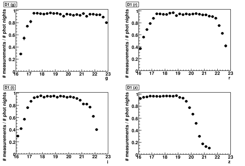
The selection is then refined by examining the contents of each star aperture. If the aperture contains pixels flagged as bad in the dead pixel maps, identified cosmics or pixels whose value is below 10 sigma below the sky background, the star measurement is rejected. At the end of this selection process, we end up with approximately 100 to 200 tertiary standard candidates per CCD, depending on the field.

The master lists of tertiary star candidates are then matched with the detection catalogs produced for each individual frame. The completeness of these catalogs varies from one epoch to another, depending on the observing conditions. Figure 16 shows the number of measurements as a function of the star magnitude for the D1 field. We see that our catalogs are complete below mag 22, 21.5, 21, and 19 for bands $g_{M}$, $r_{M}$, $i_{M}$ and $z_{M}$ respectively. Above theses magnitudes, an increasing fraction of the detections does not pass the signal-to-noise cuts ($>5$) and the calibrated magnitudes we may compute from these measurements will be biased. We therefore choose not to report calibrated magnitudes fainter than the thresholds listed above.

The last cut applied to the tertiary star candidates is based on their variability: at the end of the calibration process, we examine the lightcurves of each candidate (actually, we compute the partial $\chi^{2}$ of each individual calibrated measurement around the average calibrated magnitude) and reject all the objects which display a dispersion above a given threshold.

11.2 Building the Tertiary Catalogs

The flux of the field stars are measured using the photometry algorithms described in §4. We use the exact same algorithms that were used to measured the standard star fluxes. In practice, we use adaptive apertures of 7.5 seeing (14 pixels on average). The measured fluxes are divided by the exposure time reported in the image headers with a precision of 3 milliseconds, and then transposed to an airmass of 1 using the extinction coefficients reported in table 6. The effect of varying airmass on the $g_{M},r_{M},i_{M}$ and $z_{M}$ effective passbands is very small (below 5Å in the 1.0 - 1.6 airmass range). Therefore, no second-order airmass-color correction was applied. No evidence for such an effect was found in the calibration residuals. Finally, we compute the so-called “hat instrumental magnitudes” de-applying the Elixir uniformity maps, and applying the $\delta zp({\mathbf{x}})$ as described in §6.

The science exposures are taken in sequences of 5 to 10 exposures, depending on the band. These measurements are merged in order to produce one single list of averaged magnitudes per night. The merging procedure selects one exposure of the sequence as a reference, and allows for one free photometric alignment factor for each exposure. This permits to account for the atmospheric extinction variations during the sequence, as well as additional effects, such as fluctuations of the image quality, inducing variations of the aperture corrections. We found that on most nights, the fluctuations from one exposure to another do not exceed 0.3%.

The Local Natural Magnitudes described in the previous section are then computed using the night and band zero-points, the photometric grid maps $\delta k({\mathbf{x}})$, the grid reference colors and the MegaCam colors of the fundamental standard (namely BD +17 4708). At this stage, we have a lightcurve for each selected tertiary star, with observations taken at 20 epochs on average, spanning a time range of 3 years. All the calibrated measurements of each selected tertiary star, in each band are then averaged, in order to produce the tertiary catalogs. This averaging process is iterative: it comprises several outlier rejection steps, and attempts to identify the non-photometric nights, as described below. In the following of this section, we detail the most important points of the procedure.

11.3 Photometric Error Model

The uncertainties estimated by the photometric algorithm, reflect only the Poissonian fluctuations of the background and star photon counts. They do not account for fluctuations of the seeing and atmospheric transmission from one exposure to another. As a consequence, the uncertainties affecting the bright stars are underestimated. Since we do perform an outlier rejection while averaging the night fluxes, it is essential to build a realistic error model.

The uncertainties $\sigma_{\phi}$ affecting each measurement $\phi$ can be classically parametrized as:

$$\sigma_{\phi}=a\ \sqrt{\phi}\ \oplus\ b\ \phi\ \oplus\ c$$ (15)

where $\oplus$ is the quadratic summation symbol. The first term is the stochastic Poisson noise. The second term describes all the multiplicative fluctuations from one exposure to another, such as the atmospheric extinction, the aperture correction variations and the flat-field noise. The last term accounts for all the fluctuations which are independent of the flux, primarily the background subtraction residuals. The $a,b$ and $c$ coefficients are fitted on the data for each night, in each band. On photometric nights, the typical values of the $b$ coefficient is $0.002$. This gives an estimate of the photometric repeatability on short time scales, in photometric conditions.

11.4 Outlier Rejection

The calibrated measurements being averaged are polluted by a small fraction of outliers, usually due to CCD defects or cosmics. The outlier rejection algorithm is based on the comparison of the partial $\chi^{2}$ of each individual measurement, object or night, compared to the $\chi^{2}$ value we could expect from a 5-$\sigma$ measurement, object or night. The expected 5-$\sigma$ cut is computed in a robust way, from the median value of the individual measurements.

Additional procedures were implemented, in order to identify the “non-photometric nights”, as well as the variable stars.

11.5 Photometric Night Selection

As noted in §3, the calibration exposures are often taken several hours before or after the science exposures. The atmospheric transparency may therefore vary significantly between both sets of exposures. However the SNLS dataset is exceptional in the sense that each field was observed on a very large number of epochs, with the calibration and science images taken in many different configurations (different times in the night, variable time intervals between the science and calibration exposures). This ensures that the atmospheric transparency variations affect similarly the calibration and science exposures. Therefore, these variations can be treated just like an additional source of noise —once we have identified the pathological nights, displaying variations of more than 10%, or suffering from a large amount of absorption.

The night selection was performed as follows: first, the nights which are obviously affected by a large absorption, i.e. whose fitted zero-points depart from the average zero-points measured on the neighboring nights by more than 0.1 mag are identified and removed. Then, the nights containing a science exposure sequence which is non photometric, i.e. presenting an exposure-to-exposure variation greater than 1% are also rejected.

After having applied those two cuts, we are left with two sets of nights. The first set contains the nights during which a large number of calibration exposures was taken, over a large time range ($>3$ hours). The second set contains the nights with calibration exposures concentrated at a given time. The long term photometric stability of the first set of nights can be estimated directly by measuring the dispersion of the zero-points determined on each calibration exposure. The photometric stability of the second set cannot be estimated likewise; instead, since the dispersion of the calibrated magnitudes around their mean can be measured, we can identify and reject the non-stable nights from science data only.

Tertiary catalogs were built using (1) the first set of nights, rejecting those which display a zero-point stability worse than 1% and (2) the same nights plus the nights from the second set, the pathological nights being identified and removed, using the calibration residuals. Table 8 summarizes the number of nights flagged as photometric for both sets, and the measured dispersion of the calibration residuals. This dispersion of about 1% is mainly due to the atmospheric variations. As we can see, the dispersion is about the same in both sets of nights. With the larger set however, the statistical gain on the precision on the mean calibrated magnitudes is significant. Moreover, the mean differences between the magnitudes computed with each set of nights are compatible with the expected dispersion, which shows that no non-photometric night has been accidentally left in the larger set. As a consequence, the tertiary catalogs released with this paper are the ones built with the larger set. In all fields, the uncertainty due to the atmospheric absorption variations is of about 0.002 mag in $g_{M},r_{M},i_{M}$ and 0.003 mag in $z_{M}$.

Table 8: Night-to-night dispersion, number of nights and resulting statistical uncertainty for night sets 1 & 2.

		Set #1			Set #2
field	band	$\sigma$	# nights	$\sigma/\sqrt{N}$	$\sigma$	# nights	$\sigma/\sqrt{N}$
D1	$g$	0.007	13	0.002	0.009	28	0.002
	$r$	0.009	14	0.002	0.007	32	0.001
	$i$	0.007	11	0.002	0.009	36	0.002
	$z$	0.014	11	0.004	0.014	19	0.003
D2	$g$	0.007	8	0.003	0.007	13	0.002
	$r$	0.006	12	0.002	0.007	21	0.002
	$i$	0.004	7	0.002	0.008	25	0.002
	$z$	0.011	3	0.006	0.010	10	0.003
D3	$g$	0.002	15	0.002	0.009	29	0.002
	$r$	0.007	18	0.002	0.009	34	0.002
	$i$	0.006	14	0.002	0.013	40	0.002
	$z$	0.009	3	0.005	0.011	10	0.003
D4	$g$	0.008	18	0.002	0.009	30	0.002
	$r$	0.006	16	0.002	0.007	34	0.001
	$i$	0.006	11	0.002	0.008	29	0.002
	$z$	0.007	7	0.003	0.013	19	0.003

11.6 Results

The Local Natural Magnitudes of the tertiary standard are listed in appendix in tables LABEL:tab:d1_tertiaries, LABEL:tab:d2_tertiaries, LABEL:tab:d3_tertiaries and LABEL:tab:d4_tertiaries. We also report the corresponding $\delta k({\mathbf{x}})$ grid coefficients at the mean focal plane position where the star was observed, so that the Uniform Magnitudes can be computed from the Local Magnitudes.

(a) $r_{M}-i_{M}\ vs.g_{M}-r_{M}$

(b) $r_{M}-i_{M}\ vs.g_{M}-r_{M}$ (profile)

Figure 17: Left: $r_{M}-i_{M}$ versus $g_{M}-r_{M}$ color-color plot of the tertiary standards (Uniform Magnitudes). The agreement between all fields is good, and the contamination of non-stellar objects seems to be very low. Right: a zoom on the blue branch of the same color-color plot, after subtraction of the mean slope. We see that the colors of all four fields agree at the percent level.

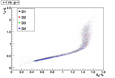
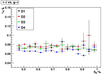
Figure 17 shows the $r_{M}-i_{M}vs.g_{M}-r_{M}$ color-color plot for all four SNLS fields. Since we are comparing objects over the whole focal plane, this figure was produced using Uniform Magnitudes instead of Local Natural Magnitudes. As we can see, the color distributions of the four SNLS fields are compatible at the 1%-level. Note that larger field-to-field differences in the stellar loci would not necessarily suggest a drift of the calibration. Indeed, we have verified using the Phoenix / GAIA library that larger effects, up to 4 to 6% may be observed due, for example, to systematic differences in the star metallicities.

As can be seen on figure 17, the MegaCam magnitude system defined in this paper is close to a Vega-based system. Indeed, it is tied to Landolt through quasi-linear color relations. Note however that our magnitudes probably depart from true Vega magnitudes by a few percents, and the amplitude of this departure is not known with precision. Other surveys, such as the Sloan Digital Sky Survey (SDSS) use a different calibration path and report magnitudes in an almost AB-system. Hence, the MegaCam magnitudes differ from SDSS magnitudes by (1) a small color term due to small differences in the effective passbands and (2) a constant term, which accounts for the differences between a AB- and a Vega-like system (see appendix G for more details).

11.7 Statistical Uncertainties

Figure 18: Average random uncertainties as a function of the magnitudes for the SNLS DEEP fields, in the $g_{M},r_{M},i_{M}$ and $z_{M}$-bands.

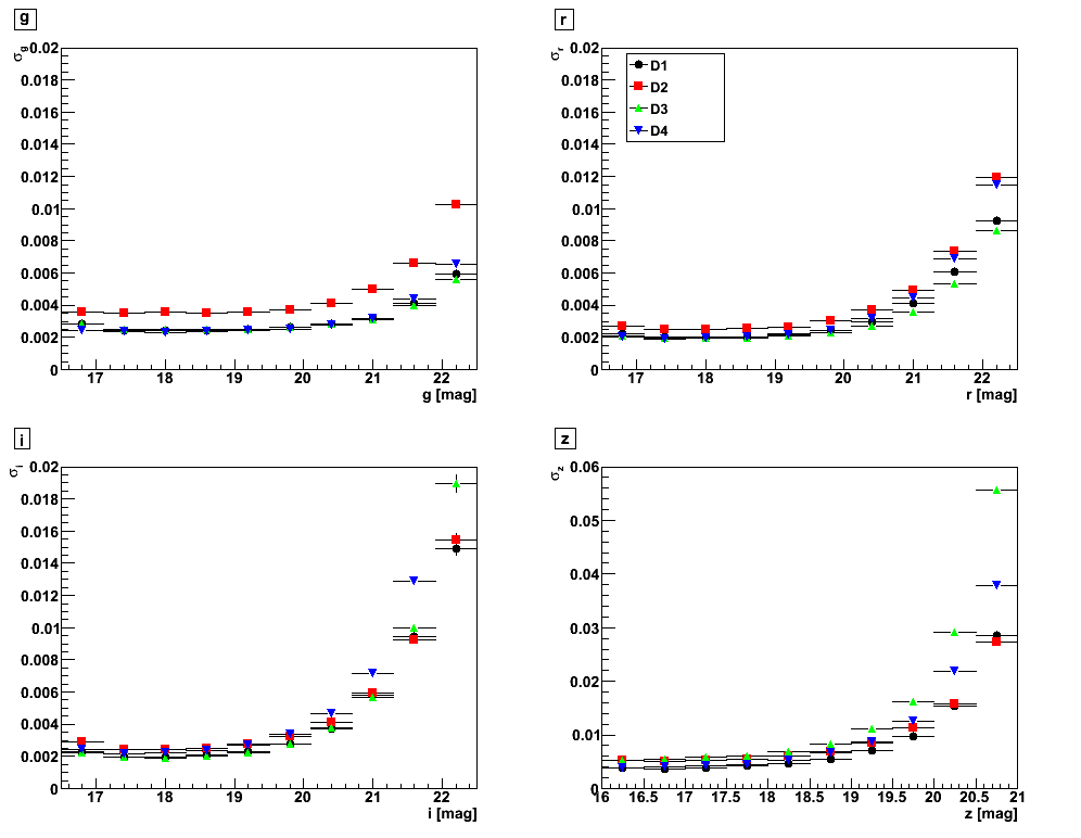
The statistical uncertainties affecting the tertiary standard calibrated fluxes comprise four independent components: (1) the tertiary standard flux measurement uncertainties —photon noise, flatfield noise and readout noise— (2) the atmospheric transparency variations between the science and calibration exposures (3) the intrinsic zero-points uncertainties and (4) the Landolt-to-MegaCam color transformation uncertainties. In this section, we shall discuss the impact of each contribution.

As discussed in the previous sections, we are interested in the uncertainties affecting the tertiary standard relative fluxes. Inspecting equation 9, we see that they are essentially equal to the statistical uncertainties on the differences between the tertiary standard calibrated magnitudes and the MegaCam magnitudes of BD +17 4708: $g_{|{\mathbf{x}}}-g_{ref}$, …$z_{|{\mathbf{x}}}-z_{ref}$.

Table 8 summarizes the night-to-night dispersion affecting the calibrated tertiary fluxes. These dispersions are mainly attributed to the atmospheric transparency variations between the calibration and science exposures. We have looked for systematic variations of the atmospheric transparency as a function of the time of the night (§12) and concluded that we can safely assume these variations to be independent from night to night. Hence, we derive a statistical uncertainty by dividing the measured dispersion by the square root of the number of photometric nights. The resulting uncertainties are of about 0.002 mag in $g_{M},r_{M},i_{M}$ and 0.003 in $z_{M}$.

The intrinsic zero-point uncertainties are of about 0.003 in the $g_{M},r_{M},$ and $i_{M}$-bands and 0.005 in the $z_{M}$-band. Given the large number of epochs, the resulting statistical error is lower than 0.001 mag in the $g_{M},r_{M},i_{M}$-bands and of about 0.001 mag in the $z_{M}$-band.

The uncertainties reported along with the calibrated magnitudes of the tertiaries (see tables LABEL:tab:d1_tertiaries, LABEL:tab:d2_tertiaries, LABEL:tab:d3_tertiaries and LABEL:tab:d4_tertiaries in appendix E) combine the uncertainties related to the photon-noise, zero-point and atmospheric variations. They are shown on figure 18. In the $g_{M},r_{M}$ and $i_{M}$-bands, for stars brighter than 20, they are dominated by the night-to-night atmospheric dispersion reported in table 8, and then by photon noise. In the $z_{M}$-band, the photon noise dominates for stars fainter than about 18.5. This is expected given the low quantum efficiency of the MegaCam detectors in the red.

The last cause of statistical uncertainties are the Landolt-to-MegaCam color transformations which impact the $g_{|{\mathbf{x}}}-g_{BD\leavevmode\nobreak\ +17\leavevmode\nobreak\ 4708}$, …$z_{|{\mathbf{x}}}-z_{BD\leavevmode\nobreak\ +17\leavevmode\nobreak\ 4708}$ magnitude differences. Since we fit global color transformations, these uncertainties are correlated and do not average out, whatever the number of epochs. We found them to be equal to $0.002$ mag in $g_{M}$, $0.0015$ mag in $r_{M}$, $0.0012$ in $i_{M}$ and $0.005$ in $z_{M}$. This is the dominant contribution to the statistical uncertainty budget.

12 Systematic Uncertainties

The systematic uncertainties that affect the calibrated fluxes are summarized in table 12.

12.1 Photometry Related Errors

As discussed in §4, we use variable size apertures to measure the flux of the calibration and tertiary stars. We do not expect the PSF to be identical on the science exposures, which are long guided exposures, and calibration exposures of much shorter exposure time, not guided, and slightly defocused. We found that on average, the seeing measured on the calibration exposures is higher than the seeing measured on the science exposures by about 0.13 arcseconds. We also have evidence that the shape of the PSF is different. As described in §4.3, we also have computed the fractional increase of flux between our standard apertures and apertures twice as large. The differences between these science image aperture corrections minus the calibration image aperture corrections are summarized in table 9. On average, we collect 0.2% more photons on the science images than on the calibration images. The tertiary star magnitudes are corrected for this effect. The residual systematic uncertainties are well below 0.001 mag.

Table 9: Aperture correction differences between the science and calibration exposures, in the sense science minus calibration exposures.

band	$\delta{\rm aper}$
$g_{M}$	$+0.0027\pm 0.0003$
$r_{M}$	$+0.0026\pm 0.0004$
$i_{M}$	$+0.0020\pm 0.0003$
$z_{M}$	$+0.0020\pm 0.0005$

12.2 The Airmass Corrections

As described in §8, the airmass dependent term is modeled as a linear correction, neglecting the second order corrections, of the form: $k^{\prime}\times(X-1)\times{\rm color}$. The second order coefficients can be modeled using synthetic photometry. Their theoretical values are summarized in table 10. Neglecting the second order correction result in a bias equal to:

$$k^{\prime}\times(X-1)\times\Bigl{[}<{\rm color}_{science}>-<{\rm color}_{Landolt}>\Bigr{]}$$

The values of these biases are listed in table 10. As we can see, they are smaller than 0.001 mag in all bands. We therefore ignore them in the systematic error budget.

Table 10: Synthetic second order airmass corrections.

band	color	$k^{\prime}$	$<{\rm color}>$	$<{\rm color}>$	bias a
	index	(synth)	(Landolt)	(tertiaries)
$g_{M}$	$g-r$	$-0.014$	$+0.735$	$+0.950$	$<0.001$
$r_{M}$	$r-i$	$-0.005$	$+0.408$	$+0.618$	$<0.001$
$i_{M}$	$r-i$	$<0.001$	$+0.408$	$+0.618$	$<0.001$
$z_{M}$	$i-z$	$<0.001$	$+0.192$	$+0.272$	$<0.001$

• Effects on the tertiary magnitudes of neglecting the second order correction. The resulting bias is smaller than 0.001 mag in all bands.

12.3 The Shutter Precision

As described in §2, the actual exposure time is measured using a dedicated system with a precision of 0.001 second. The shutter ballistics was investigated by the CFHT team using sequences of exposures of the same field, taken with increasing exposure times. Cuillandre (2005) showed that the specification of 3 ms was actually met. The study could not measure a systematic shutter uncertainty. In order to be conservative, we assign an error of 3 ms to all the exposure times. This error is negligible for the science exposures, but not for the calibration exposures, of mean exposure time $T_{exp}\sim 2$ s. Being conservative, we consider that this induces a systematic error on the tertiary magnitudes, of $0.0015$ mag (correlated) in all bands.

12.4 Landolt Catalog Internal Dispersion

The Landolt (1992b) catalog is known to be remarkably uniform, with a reported internal dispersion of 0.003 mag. We have checked this assertion, and estimated the resulting error on the tertiary magnitudes. Indeed, we observe regularly 8 Landolt fields, containing about $250$ Landolt stars and representing a little less than half of the whole Landolt catalog. Since each SNLS field is itself calibrated with a subset of no more than the three or four Landolt fields that are observable along with it, we can expect to measure a sizeable error due to the Landolt catalog internal dispersion.

The field-to-field dispersion of the zero-points was measured on the stable nights during which more than one Landolt field was observed. We have measured it to be of 0.002 mag in $gri$ and 0.004 in $z$. Since each SNLS field is calibrated with about 4 different Landolt fields on average, we estimate the uncertainty to be of about 0.001 mag in the $gri$-bands and 0.002 mag in the $z$-band.

12.5 Grid Reference Colors

As discussed in §6, there is a hidden color reference associated to each $\delta zp({\mathbf{x}})$ map. The grid sequences were calibrated using the average run zero-points provided by the Elixir pipeline. These zero-points are valid for an entire run (about two weeks), and do not account for the night-to-night variations. We have evaluated the night-to-night dispersion of the zero-points to be of about $\sigma_{n-to-n}\sim 0.01-0.02\ {\rm mag}$. The grid reference colors are known to this precision, and each $\delta zp({\mathbf{x}})$ map pixel is therefore affected by an error, equal to $\delta k({\mathbf{x}})\times\sigma_{n-to-n}$. Table 11 summarizes the largest associated uncertainty.

Table 11: Uncertainties on the grid reference colors and the associated max error affecting the grid pixels.

band	color	$\max_{\mathbf{x}}\left[\delta k({\mathbf{x}})\right]$	$\sigma_{\rm color}$	max grid error
$g_{M}$	$g-r$	0.04	0.021	$<0.001$
$r_{M}$	$r-i$	0.04	0.013	$<0.001$
$i_{M}$	$r-i$	0.05	0.013	$<0.001$
$z_{M}$	$i-z$	0.06	0.019	$<0.001$

12.6 Adequacy of the Grid Color Corrections

The agreement of the MegaCam passband model and the grid corrections has been discussed in 7.3. We have found that there is an excellent agreement between the synthetic color terms determined using the Pickles (1998) library and the color terms measured from the grid corrections, except in the $r_{M}$-band, where there might be a slight disagreement. We found, using the real spatial distribution of the Landolt star measurements, that the differences between the model predictions and grid measurements have an impact of less than 0.001 mag on the zero-points in the $g_{M}$, $i_{M}$ and $z_{M}$-bands, and of 0.002 mag in the $r_{M}$-band.

12.7 The Magnitudes of BD +17 4708

BD +17 4708 is too bright to be observed directly with MegaCam. Its MegaCam magnitudes were determined indirectly in §9. The uncertainties on these estimates are dominated by astrophysical considerations, especially the impact of the fact that BD +17 4708 is possibly a binary system.

12.8 The SED of BD +17 4708

The last source of systematic uncertainties that must be discussed is related to the measurement of the SED of BD +17 4708. We use version 2 of the determination published by Bohlin & Gilliland (2004a), available on the CALSPEC web site. The uncertainties affecting this measurement come from two sources. First, the repeatability of the STIS observations, which is routinely monitored with repeated observations of the star AGK +81 266. According to figure 1 of Bohlin & Gilliland (2004a) this repeatability is of about 0.3% in the $g_{M}$-, $r_{M}$-, $i_{M}$- and and 0.6% in the $z_{M}$-bands respectively (1 $\sigma$ errors). There are hints that there are correlations between these uncertainties. We have computed our own repeatability model using the original monitoring spectra of AGK +81 266, integrated in the MegaCam passbands. We found a repeatability of 0.2%, 0.3%, 0.3% and 0.6% in the $g_{M}$-, $r_{M}$-, $i_{M}$- and $z_{M}$-bands respectively, with strong correlations between the neighboring bands.

The other main source of uncertainty come from the model flux distributions of the three primary standards themselves. This includes internal uncertainties of the NLTE white dwarf atmosphere modeling, as well as uncertainties in the determination of the star metallicities, surface gravity and effective temperature, from the observation of the Balmer line profiles. From the results presented in Bohlin (2002), we adopt a 0.5% uncertainty (1 $\sigma$) over the range 3000Å- 10000Å. This translates into uncertainties on the $g_{M}$, $r_{M}$, $i_{M}$ and $z_{M}$ synthetic broadband fluxes of BD +17 4708, relative to the synthetic $V$-band flux, which are essentially negligible, except for the $i_{M}$- and $z_{M}$-bands (0.15% and 0.24% respectively).

The sum of the two contributions is dominated by the repeatability of the STIS instrument. Combining both sources of uncertainties, we obtain the covariance matrix listed in appendix D, table 21.

Table 12: Summary of the systematic uncertainties affecting the calibrated magnitudes and fluxes.

	$g_{M}$	$r_{M}$	$i_{M}$	$z_{M}$
Aperture corrections	$<0.001$	$<0.001$	$<0.001$	$<0.001$
Background subtraction	$<0.001$	$<0.001$	$\pm 0.005$	$<0.001$
Shutter precision	$\pm 0.0015$	$\pm 0.0015$	$\pm 0.0015$	$\pm 0.0015$
Linearity	$<0.001$	$<0.001$	$<0.001$	$<0.001$
Second order airmass corrections	$<0.001$	$<0.001$	$<0.001$	$<0.001$
Grid Reference Colors	$<0.001$	$<0.001$	$<0.001$	$<0.001$
Grid Color Corrections	$<0.001$	$<0.001$	$\pm 0.002$	$<0.001$
Landolt catalog	$\pm 0.001$	$\pm 0.001$	$\pm 0.001$	$\pm 0.002$
Magnitudes of BD +17 4708	$\pm 0.002$	$\pm 0.004$	$\pm 0.003$	$\pm 0.018$
Total	$\pm 0.003$	$\pm 0.004$	$\pm 0.006$	$\pm 0.018$
SED of BD +17 4708	$\pm 0.001$	$\pm 0.002$	$\pm 0.004$	$\pm 0.007$
Total	$\pm 0.003$	$\pm 0.005$	$\pm 0.007$	$\pm 0.019$

12.9 Summary: the Full Uncertainty Budget

We obtain the full uncertainty budget by combining the statistical and systematic uncertainties. The full covariance matrix is listed in table 20 (appendix D). As discussed above, we have chosen to report the uncertainties that affect the quantities $g_{M}-g_{ref}$, $r_{M}-r_{ref}$, $i_{M}-i_{ref}$ and $z_{M}-z_{ref}$, i.e. the differences between the tertiary magnitudes BD +17 4708 magnitudes. Note that these quantities are correlated with the Landolt magnitudes of BD +17 4708: $U_{ref}$, $B_{ref}$, $V_{ref}$, $R_{ref}$ and $I_{ref}$. Since the SNLS cosmology analysis does compare nearby supernova $UBVRI$ magnitudes with the MegaCam magnitudes of more distant supernovae, we cannot ignore these correlations. Hence, we report a $9\times 9$ covariance matrix, containing all these correlations.

The contribution of the uncertainties affecting the measurement of the SED of BD +17 4708 are listed in table 21. Similarly, we report a $9\times 9$ covariance matrix, including the 5 Landolt bands in addition to the MegaCam bands.

13 Discussion

In this paper, we have characterized the MegaCam focal plane photometric response, built a model of the MegaCam passbands, and defined a system of Local Natural Magnitudes, depending on the focal plane position. This system is implemented as four catalogs of tertiary standard stars, one for each of the four CFHTLS DEEP field. The relations between these magnitudes and their physical flux counterparts have been explicited. They rely on a specific star, BD +17 4708, with known Landolt $UBVRI$ and MegaCam $g_{M},r_{M},i_{M}$, $z_{M}$-magnitudes, and a known Spectral Energy Distribution measured and calibrated independently by Bohlin & Gilliland (2004a).

The statistical and systematic uncertainties affecting the tertiary magnitudes and their flux counterparts have been discussed in §10.2, §11.7 and §12. The uncertainties affecting the MegaCam magnitudes of each tertiary standard may be classically split into two different contributions. First, a statistical uncertainty which accounts for the flux measurement shot noise, the number of epochs averaged and the average photometric conditions under which this star was observed. This contribution is summarized in figure 18. In the $g_{M},r_{M}$ and $i_{M}$-bands, it amounts to about 0.0025 mag for a mag 18 star and stays below 0.005 mag up to mag 21. In the $z_{M}$-band, it is higher, of about 0.005 mag for a mag 18 star, and reaches 0.01 mag for a mag 19.5 star. The second contribution is a systematic uncertainty which is summarized in the first section of table 12 and characterizes how well the MegaCam system is tied to the Landolt system: 0.002 in $g_{M}$ and $r_{M}$, 0.006 in $i_{M}$ and 0.003 in $z_{M}$. Finally, the magnitude-to-flux conversion introduces additional uncertainties, of 0.005 mag or better in the $g_{M},r_{M},i_{M}$-bands and 0.019 mag in $z_{M}$. The final systematic uncertainty budget is detailed in table 12 and in the covariance matrices 20 and 21 listed in appendix D.

In order to fully quantify how well this system is tied to Landolt, we should also add to this budget the impact of the Landolt-to-MegaCam color term uncertainties. If one considers the full relevant color range from Vega ($B-V\sim$ 0) to the mean colors of the Landolt stars ($B-V\sim 0.77$), one finds that this contribution is large, between 0.005 and 0.015 mag, depending on the band. BD +17 4708 was chosen as a fundamental standard partly because its colors are closer to the mean color of the Landolt stars. This allows one to reduce the final impact of the Landolt-to-MegaCam color term uncertainties down to less than $0.002$ mag in $g_{M},r_{M},i_{M}$ and $0.005$ mag in $z_{M}$.

The statistical and systematic error budgets are extremely similar from one field to another, mainly because each field was treated on an equal footing, with the same observation strategy. The only systematic difference from one field to another is the mean effective airmass $\sim 1.2$ for D1 and D2 and $\sim 1.3$ for D3 and D4. Propagating the uncertainties affecting the airmass coefficients determined in §8, one finds that the impact of these differences on the final tertiary magnitudes is very small, below 0.001 mag.

The MegaCam magnitudes defined in this paper are tied to the Landolt system using (quasi-)linear color relations. Hence Vega (like any A0V star) should have MegaCam colors close to zero. Note however that the Landolt and MegaCam magnitudes of Vega are affected with large uncertainties of a few percents at least. We have not been able to quantify with precision the departure of this system from a strictly Vega-based system. This is the reason why we have discarded Vega as a fundamental standard, and used BD +17 4708 instead.

We would like to stress again, that the photometric system presented in this paper has been designed in such a way that no color correction (or grid color correction) ever has to be applied to the science objects’ magnitudes. Indeed, our main goal is to keep the connection between the magnitudes reported by the survey and the underlying physical fluxes. This is especially important when dealing with non-stellar objects, such as supernovae or galaxies.

The main application of this work is the calibration of the supernova lightcurves obtained during the 3 first years of the SNLS survey. Nevertheless, we release all the necessary information so that any MegaCam dataset can be anchored to this system, provided that one of the SNLS DEEP fields is regularly observed during the program along with the science data.

The calibration of the SNLS 3-year supernova lightcurves from the tertiary catalogs presented in this paper is discussed in detail in Guy et al. (2009, in prep) and anyone interested in tying a dataset to our system should study this paper as a first step. The recommended procedure may be briefly outlined as follows:

1. first, the instrumental magnitudes of the SNLS tertiary stars used as calibrators must be measured using the exact same photometry algorithm as the one used to estimate the flux of the science objects,

2. then, the zero-points are derived by comparing the instrumental magnitudes of the tertiaries with the calibrated magnitudes released with this paper (see appendix E),

3. the Local Natural Magnitudes can then be obtained by applying those zero-points to the science objects’ instrumental magnitudes,

4. finally physical broadband fluxes may be derived from the Local Natural Magnitudes using (a) equation 9 (b) the MegaCam magnitudes of BD +17 4708 reported in table 7 (c) the SED of BD +17 4708 discussed in §10.1 and (d) the MegaCam passband model detailed in appendix B. The filter model at the exact focal plane location of the science target may be obtained by interpolating between the filter scans detailed in tables LABEL:tab:u_band_table to LABEL:tab:z_band_table.

Very recently, Landolt (2009) published an extension of the catalog used in this paper. Bluer as well as fainter stars were added to the Landolt (1992b) catalog. The author tied the measurements to his former magnitude system. Note that for a small subset of the Landolt (1992b) catalog (about 40-50 stars), revised magnitudes were published. In general the magnitude changes are small, of about 0.003 mag, except for a handful of stars (less than 10), for which they can amount to 0.01 to 0.1 mag. We have checked that, for the stars used in this analysis, the average magnitude difference between both catalogs is smaller than 0.001 mag.

The SDSS-II first year dataset (Holtzman et al., 2008) relies on a similar calibration scheme. The calibration of the SDSS SN Ia lightcurves relies on the catalog of tertiary standard stars published by Ivezić et al. (2007). This latter catalog contains about 1.01 million non-variable stars located on the SDSS equatorial stripe 82 ($|\delta_{J2000}|<1.266,20h34<\alpha<4h$) and is believed to be uniform at the 1% level. Although the reduction of drift scan imaging data poses different problems, it is interesting to note that Ivezić et al. (2007) had to solve very similar problems, such as the uniformity of the photometric response along a drift scan, or the small differences between the filters which equip each column of the camera.

The Ivezić et al. (2007) catalog is calibrated to the natural SDSS 2.5-m photometric system, which deviates from a perfect AB system by about 4% in the $u$-band, and 1 to 2% in the $griz$-bands. Therefore, Holtzman et al. (2008) chose to tie their magnitudes to the HST white-dwarf scale. Several potential CALSPEC primary standards were observed with the smaller SDSS Photometric Telescope (PT) and their magnitudes were transferred to the SDSS 2.5-m photometric system using linear color transformations, supplemented by synthetic photometry in order to determine star-specific offsets with respect to the color transformations. As in our case, the color transformations are not well-defined in the white-dwarf color range. Hence, they chose to use the three CALSPEC red, faint, solar analogs P330E, P177D and P041C as primary standards. The calibration path adopted by Holtzman et al. (2008) is extremely similar to that presented in this paper. Its main advantage is that the SDSS Photometric Telescope response is well characterized, and that the color transformations between the PT and the science telescope are smaller.

There are several shortcomings affecting the calibration presented is this paper. First, BD +17 4708 has not been observed directly with MegaCam. We therefore rely on (1) the Landolt measurements of BD +17 4708, (2) the Landolt-to-MegaCam color transformations, (3) on the Phoenix / GAIA synthetic libraries and combined with estimates of BD +17 4708’s metallicity, surface gravity and extinction to estimate its MegaCam magnitudes. Then, the time interval between the calibration and science measurements is of several hours. We are therefore sensitive to the variations of the atmospheric conditions on such long periods. The large number of epochs allows one to reduce this source of uncertainty to 2 mmags on average. However, a more robust calibration would be obtained if calibration and science observations could be separated by intervals of a few minutes only, and if repeated exposures of the same field through the observation sequence could allow one to estimate the photometricity of the observing condition, during the science and calibration observations. Finally, the current grid dataset, with observations every 6 months, does not allow one to monitor precisely the run-to-run variations of the imager photometric response.

In order to overcome these shortcomings, we have designed a dedicated calibration program, called MAPC (MegaCam Absolute Photometric Calibration). MAPC combines observations of the DEEP fields, HST spectrophotometric standards which are a little fainter than BD +17 4708, and dithered observations of the SDSS equatorial stripe 82, all taken in a little less than 30 minutes. This program will allow us to redefine the MegaCam Local Natural Magnitudes independently of the Landolt magnitudes. We also will be able to explicit the connections of the MegaCam magnitudes with the widely used SDSS magnitude system.

A second article dealing with the precise photometric calibration of MegaCam data will follow the current effort. It should be noted that the photometric precision delivered since first light by the Elixir pipeline (4%) falls within the typical scientific requirements and has not been a limitation for most users. We expect, however, that the new level of precision provided by our current work will enable science currently unforeseen with the MegaCam data set.

Appendix A Measuring the Photometric Response Maps (details)

We have shown in §6 that fitting the uniformity maps $\delta zp({\mathbf{x}})$ and $\delta k({\mathbf{x}})$ from the dithered grid field observations is a very large dimensionality problem, involving about 200,000 parameters. Of these parameters, most are the grid stars instrumental magnitudes (i.e. nuisance parameters). The grid maps are developed on independent superpixels $\delta zp({\mathbf{x}})=\sum_{k=1}^{N}\alpha_{k}p_{k}({\mathbf{x}})$, $\delta k({\mathbf{x}})=\sum_{k=1}^{N^{\prime}}\beta_{k}q_{k}({\mathbf{x}})$. The $\delta zp({\mathbf{x}})$ are fit on $512\times 512$ superpixels, with 1296 superpixels on the focal plane. The precision obtained on the $\delta k({\mathbf{x}})$ parameters depends on the color lever arm. In order to maximize it, the $\delta k({\mathbf{x}})$ maps are developed on larger ($1024\times 1537$) superpixels, with only 216 superpixels on the focal plane. Since both maps have a reference cell, there are $N=1295$ and $N^{\prime}=215$ $\alpha_{k}$ and $\beta_{k}$ coefficients respectively, representing 1510 parameters in total. We have checked that first order methods, which do not require one to build the second derivatives of the $\chi^{2}$ converge very slowly and do not allow one to obtain the exact solution in a reasonable amount of iterations. In this section, we show that the structure of the problem is such that the dimensionality of the normal equations can be in fact greatly reduced. This allows us to obtain the exact solution of the problem in a single step.

First, the model fitted on the instrumental magnitudes of the grid stars is as follows. This model connects the expectation of the $j$th measured instrumental magnitude of star $i$, $m_{ADU|{\mathbf{x}}}(i,j)$ with the fit parameters, i.e. the grid map parameters $\alpha_{k}$ and $\beta_{k}$ and the magnitudes of the grid stars at the reference location, $m_{|{\mathbf{x}}_{0}}(i)$. The star colors are fixed, and recomputed iteratively until they do not vary by more than 0.0001 mag. The model can be written:

$$E\left[m_{ADU|{\mathbf{x}}}(i,j)\right] = m_{|{\mathbf{x}}_{0}}(i)+\sum_{k}\alpha_{k}p_{k}({\mathbf{x}}_{ij})+$$

$$\sum_{k}\beta_{k}q_{k}({\mathbf{x}}_{ij})\times\Bigl{(}{\rm col}_{|{\mathbf{x}}_{0}}(i)-{\rm col}_{grid}\Bigr{)}$$

Grouping together the grid map parameters $\alpha_{k}$ and $\beta_{k}$ in a single vector ${\mathbf{p}}$, and the star magnitudes in another (much larger) vector ${\mathbf{M}}$, the equation above can be rewritten in the more compact form:

$$E\left[m_{ADU|{\mathbf{x}}}(i,j)\right]={\mathbf{D}}_{ij}^{T}{\mathbf{p}}+{\mathbf{S}}_{i}^{T}{\mathbf{M}}$$ (16)

${\mathbf{D}}_{ij}$ and ${\mathbf{S}}_{i}$ are one-dimensional vectors, defined for each measurement $j$, and each star $i$. The large vector ${\mathbf{S}}_{i}$ contains a single non-zero element:

$${\mathbf{D}}_{ij}[k] = p_{k}(x_{ij})$$ (17)

$${\mathbf{D}}_{ij}[k+N] = q_{k}(x_{ij})\times{\rm color}_{i}$$ (18)

$${\mathbf{S}}_{i}[j] = \delta_{ij}$$ (19)

The $\chi^{2}$ to minimize can be written as:

$$\chi^{2}({\mathbf{p}},{\mathbf{M}})=\sum_{ij}w_{ij}\left({\mathbf{D}}_{ij}^{T}{\mathbf{p}}+{\mathbf{S}}_{i}^{T}{\mathbf{M}}-{m}_{ADU|{\mathbf{x}}}(i,j)\right)^{2}$$ (20)

where $w_{ij}$ is the weight of the measurement ${m}_{ADU|{\mathbf{x}}}(i,j)$. The associated normal equations are:

$$\begin{pmatrix}{\mathbf{W}}_{p}&{\mathbf{A}}^{T}\\ {\mathbf{A}}&{\mathbf{W}}_{M}\\ \end{pmatrix}\times\begin{pmatrix}{\mathbf{p}}\\ {\mathbf{M}}\\ \end{pmatrix}=\begin{pmatrix}{\mathbf{B}}_{p}\\ {\mathbf{B}}_{M}\\ \end{pmatrix}$$ (21)

where

$${\mathbf{W}}_{p} = \sum_{ij}\ w_{ij}\ {\mathbf{D}}_{ij}\ {\mathbf{D}}_{ij}^{T}$$ (22)

$${\mathbf{W}}_{M} = \sum_{ij}\ w_{ij}\ {\mathbf{S}}_{i}\ {\mathbf{S}}_{i}^{T}$$ (23)

$${\mathbf{A}} = \sum_{ij}\ w_{ij}\ {\mathbf{S}}_{i}\ {\mathbf{D}}_{ij}^{T}$$ (24)

and

$${\mathbf{B}}_{p} = \sum_{ij}\ w_{ij}\ m_{ADU|{\mathbf{x}}}(i,j)\ {\mathbf{D}}_{ij}$$ (25)

$${\mathbf{B}}_{M} = \sum_{ij}\ w_{ij}\ m_{ADU|{\mathbf{x}}}(i,j)\ {\mathbf{S}}_{i}$$ (26)

Since all coordinates but one of each vector ${\mathbf{S}}_{i}$ are zero, all the matrices ${\mathbf{S}}_{i}{\mathbf{S}}_{i}^{T}$ are diagonal. Hence ${\mathbf{W}}_{M}$ is diagonal. We can eliminate ${\mathbf{M}}$ from the above normal equations:

$$\left({\mathbf{W}}_{p}-{\mathbf{A}}^{T}{\mathbf{W}}_{M}^{-1}{\mathbf{A}}\right){\mathbf{p}}={\mathbf{B}}_{p}-{\mathbf{A}}^{T}{\mathbf{W}}_{M}^{-1}{\mathbf{B}}_{M}$$ (27)

and get a computationally tractable equation because ${\mathbf{W}}_{M}^{-1}$ is diagonal. This linear equation has the dimensionality of ${\mathbf{p}}$ and can be solved for ${\mathbf{p}}$. ${\mathbf{M}}$ can then be determined from:

$${\mathbf{M}}={\mathbf{W}}_{M}^{-1}\Bigl{(}{\mathbf{B}}_{M}-{\mathbf{A}}{\mathbf{p}}\Bigr{)}$$ (28)

using again that ${\mathbf{W}}_{M}$ is diagonal.

Equations 27 and 28 yield the exact solution of the linear least squares problem (20). Besides reaching the least squares minimum, the method described here provides us with the true covariance matrix of the calibration parameters. Indeed, one can show from equation (21) that the full covariance matrix, marginalized over the grid star magnitudes is given by:

$${\mathbf{C}}=\left({\mathbf{W}}_{p}-{\mathbf{A}}^{T}{\mathbf{W}}_{M}^{-1}{\mathbf{A}}\right)^{-1}$$ (29)

What allowed us to reduce the dimensionality of the problem and obtain the exact solution is the very specific structure of the $\chi^{2}$ second derivative matrix, which contained a very large diagonal sub-block. Such a structure seems to be very common in calibration problems, such as the ones described in Kaiser et al. (1999); Padmanabhan et al. (2008). This structure can be observed when we can distinguish a set of global parameters (here, the grid map parameters), combined with another much larger set of local parameters (here, the magnitudes). The key feature of the least-squares problem that makes it eligible for this technique is that no $\chi^{2}$ term contains two elements of ${\mathbf{M}}$. The same procedure still applies if the $m_{i}$ are vectors, with the difference that ${\mathbf{W}}_{M}$ is block-diagonal. In those cases, the factorization described here can be used, making the problem tractable or at least saving large amounts of computing time.

Appendix B MegaCam Passbands

In this section, we detail our model of the ingredients of the MegaCam effective passbands, presented in §7 and summarized on figure 19. For all bands, the model consists in the product of five components:

$$T(\lambda;{\mathbf{x}})=T_{f}(\lambda;{\mathbf{x}})\times T_{o}(\lambda)\times R_{m}(\lambda)\times T_{a}(\lambda)\times\varepsilon(\lambda)$$ (30)

$T_{f}(\lambda;{\mathbf{x}})$ is the position dependent transmission of the interference filters. $T_{o}(\lambda)$ is the transmission of the four lens optical system which equip MegaPrime. It also includes the transmission of the camera window. $R_{m}(\lambda)$ refers to the reflectivity of the primary mirror. $T_{a}(\lambda)$ is the average transmission of the atmosphere above Mauna Kea. Finally, $\varepsilon(\lambda)$, is the mean quantum efficiency of the E2V CCDs which equip the focal plane of MegaCam.

Figure 19: MegaCam effective passbands at the center of the focal plane (filled) and close to the sides of the focal plane (solid gray lines). As discussed in §6, the filters are bluer on the edges than at the center of the camera. We also display the cumulative effect of the main ingredients of the effective passbands: average quantum efficiency of the MegaCam CCDs $\epsilon(\lambda)$, mirror reflectivity $T_{m}(\lambda)$, transmission of the wide field adapter optics (including the camera window) $T_{o}(\lambda)$, and average atmospheric transmission $T_{a}(\lambda)$. The mirror reflectivity is essentially flat, and does not impact the passband shape. In the $z_{M}$-band, the red cutoff is determined by the quantum efficiency curve. The blue side of the $u_{M}$-band is shaped by the quantum efficiency curve as well as the optics and atmospheric transmissions, however the cutoff itself seems to be determined by the filter transmission.

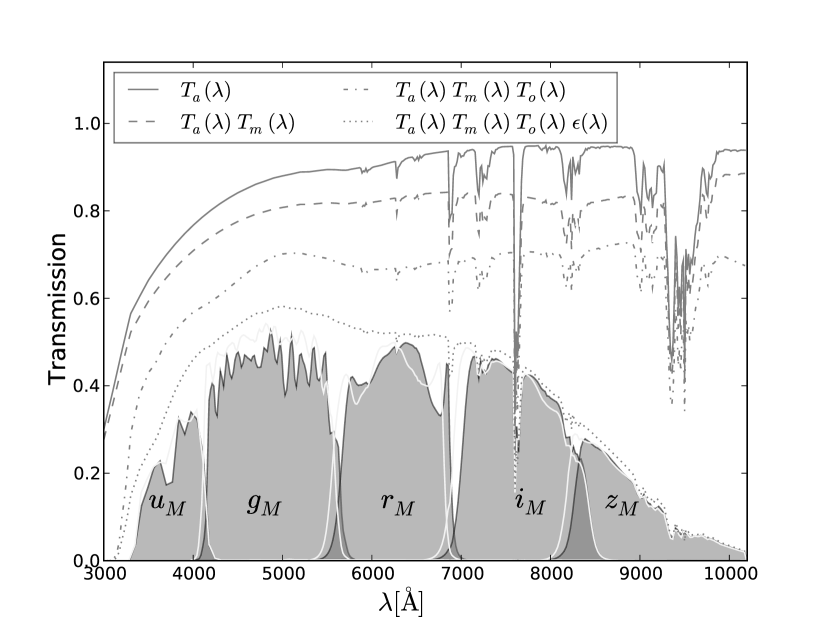
The transmission of the optical system, $T_{o}(\lambda)$ and the reflectivity of the primary mirror, $R_{m}(\lambda)$ were obtained from the CFHT team. The quantum efficiency $\varepsilon(\lambda)$ of the camera was obtained from the CEA team. It is actually an average model, derived from the measured quantum efficiencies of the chips which equip MegaCam. The Mauna Kea atmospheric transmission $T_{a}(\lambda)$ is being measured by the Nearby Factory Collaboration using the SuperNova Integral Field Spectrometer (Buton & SNfactory Collaboration 2009). We use a preliminary version of this measurement. Finally, the $O_{2}$ and $OH$ absorption lines have a sizeable impact on the $z_{M}$ passband. We use the determination presented in Hinkle et al. (2003). The resolution of the original determined being of about 0.15 Å, we have rebinned it, with to reach a bin size of about 3Å. Table 13 displays the product of all the components listed above.

Finally, the filter transmissions, $T_{f}(\lambda,{\mathbf{x}})$, were characterized by their manufacturer (Sagem / REOSC). For each filter, ten scans were performed at ten different locations — namely, at the center of the filter, and then, at 23, 47, 70, 93, 117, 140, 163, 186 and 210 millimeters from the center, along a diagonal. The transmissions reported by Sagem / REOSC were blueshifted as described in §7, in order to account for the fact that the f/4 beam does not cross the filters at a normal incidence on average. The resulting blueshifted transmissions $u_{M},g_{M},r_{M},i_{M},$ and $z_{M}$ are reported in tables LABEL:tab:u_band_table, LABEL:tab:g_band_table, LABEL:tab:r_band_table, LABEL:tab:i_band_table and LABEL:tab:z_band_table respectively. In order to build a passband model which is continuous as a function of the position, the scans presented in those tables were interpolated, assuming a central symmetry around the focal plane center, as indicated by the $\delta k({\mathbf{x}})$ maps.

The sidereal positions of the objects can be mapped to “filter coordinates” (in millimeters), using the following formula:

$$x_{f} = F\times\Bigl{[}\cos(\delta)\ \sin(\alpha-\alpha_{0})\Bigr{]}$$

$$y_{f} = F\times\Bigl{[}-\cos(\delta)\sin(\delta_{0})\cos(\alpha-\alpha_{0})+\sin(\delta)\cos(\delta_{0})\Bigr{]}$$ (31)

where $(x_{f},y_{f})$ are the point coordinates in the filter frame (expressed in millimeters), $F$ is the MegaPrime focal length (14,890 millimeters), $(\alpha,\delta)$ and $(\alpha_{0},\delta_{0})$ are the sidereal position of the object and the field center respectively. In the formula above, we use the fact that the distance between the filters and the focal plane is negligible compared to the focal length.

13

Table 13: Open Transmission of the MegaCam imager (no filters)

$\lambda$	transmission
$(\AA)$
…	…
3100.0	0.0013
…	…
4100.0	0.4817
…	…
5100.0	0.5764
…	…
6100.0	0.5190
…	…
7100.0	0.4976
…	…
8100.0	0.3705
…	…
9100.0	0.1394
…	…
10100.0	0.0272
…	…

14

Table 14: $u_{M}$ filter scan

$\lambda$	$T_{u_{M}}(\lambda;r)$	$T_{u_{M}}(\lambda;r)$	$T_{u_{M}}(\lambda;r)$	$T_{u_{M}}(\lambda;r)$	$T_{u_{M}}(\lambda;r)$	$T_{u_{M}}(\lambda;r)$	$T_{u_{M}}(\lambda;r)$	$T_{u_{M}}(\lambda;r)$	$T_{u_{M}}(\lambda;r)$	$T_{u_{M}}(\lambda;r)$
$(\AA)$	$r=0\ \rm{mm}$	$r=23\ \rm{mm}$	$r=47\ \rm{mm}$	$r=70\ \rm{mm}$	$r=93\ \rm{mm}$	$r=117\ \rm{mm}$	$r=140\ \rm{mm}$	$r=163\ \rm{mm}$	$r=186\ \rm{mm}$	$r=210\ \rm{mm}$
3275	0.0000	0.0000	0.0020	0.0000	0.0000	0.0000	0.0000	0.0000	0.0000	0.0000
3280	0.0000	0.0000	0.0041	0.0023	0.0020	0.0000	0.0000	0.0001	0.0001	0.0002
3285	0.0000	0.0020	0.0052	0.0048	0.0040	0.0021	0.0019	0.0019	0.0023	0.0024
3290	0.0019	0.0043	0.0068	0.0062	0.0052	0.0044	0.0039	0.0040	0.0048	0.0052
3295	0.0041	0.0056	0.0091	0.0083	0.0068	0.0057	0.0051	0.0052	0.0063	0.0069
3300	0.0054	0.0075	0.0125	0.0113	0.0091	0.0076	0.0067	0.0069	0.0086	0.0094
3305	0.0073	0.0103	0.0174	0.0156	0.0124	0.0103	0.0090	0.0093	0.0118	0.0130
3310	0.0100	0.0144	0.0247	0.0221	0.0173	0.0142	0.0123	0.0129	0.0164	0.0181
3315	0.0139	0.0203	0.0355	0.0317	0.0247	0.0200	0.0173	0.0180	0.0229	0.0252
3320	0.0196	0.0290	0.0512	0.0458	0.0354	0.0285	0.0244	0.0254	0.0321	0.0351
3325	0.0280	0.0417	0.0740	0.0661	0.0510	0.0408	0.0347	0.0360	0.0449	0.0488
3330	0.0400	0.0598	0.1055	0.0944	0.0730	0.0582	0.0492	0.0506	0.0624	0.0671
3335	0.0574	0.0856	0.1479	0.1331	0.1038	0.0828	0.0696	0.0708	0.0862	0.0921
3340	0.0822	0.1211	0.2022	0.1834	0.1450	0.1163	0.0975	0.0981	0.1182	0.1257
3345	0.1158	0.1671	0.2651	0.2429	0.1961	0.1589	0.1336	0.1338	0.1596	0.1687
3350	0.1605	0.2242	0.3341	0.3096	0.2564	0.2116	0.1797	0.1796	0.2123	0.2233
3355	0.2168	0.2907	0.4043	0.3795	0.3234	0.2735	0.2359	0.2364	0.2762	0.2887
3360	0.2829	0.3627	0.4702	0.4474	0.3933	0.3415	0.3010	0.3031	0.3485	0.3623
3365	0.3558	0.4362	0.5287	0.5099	0.4631	0.4142	0.3740	0.3781	0.4268	0.4409
3370	0.4292	0.5027	0.5757	0.5630	0.5270	0.4860	0.4494	0.4554	0.5040	0.5171
3375	0.4964	0.5567	0.6092	0.6038	0.5812	0.5510	0.5217	0.5300	0.5739	0.5848
3380	0.5519	0.5962	0.6298	0.6319	0.6233	0.6059	0.5862	0.5963	0.6319	0.6400
3385	0.5923	0.6211	0.6404	0.6484	0.6514	0.6469	0.6369	0.6481	0.6732	0.6794
3390	0.6169	0.6341	0.6440	0.6557	0.6670	0.6719	0.6700	0.6806	0.6979	0.7042
3395	0.6300	0.6391	0.6434	0.6572	0.6740	0.6850	0.6891	0.6981	0.7130	0.7206
3400	0.6316	0.6365	0.6382	0.6528	0.6726	0.6877	0.6950	0.7042	0.7223	0.7311
3405	0.6237	0.6275	0.6282	0.6437	0.6650	0.6827	0.6925	0.7049	0.7281	0.7363
3410	0.6100	0.6145	0.6161	0.6318	0.6541	0.6732	0.6868	0.7043	0.7294	0.7355
3415	0.5954	0.6017	0.6053	0.6209	0.6430	0.6641	0.6815	0.7036	0.7250	0.7305
3420	0.5841	0.5923	0.5975	0.6132	0.6354	0.6581	0.6778	0.7010	0.7185	0.7269
3425	0.5761	0.5850	0.5919	0.6076	0.6298	0.6529	0.6734	0.6942	0.7156	0.7303
3430	0.5694	0.5777	0.5853	0.6008	0.6228	0.6459	0.6655	0.6863	0.7219	0.7432
3435	0.5636	0.5705	0.5778	0.5925	0.6140	0.6364	0.6565	0.6832	0.7390	0.7634
3440	0.5617	0.5668	0.5739	0.5868	0.6064	0.6286	0.6528	0.6910	0.7622	0.7838
3445	0.5694	0.5735	0.5804	0.5906	0.6073	0.6305	0.6611	0.7123	0.7835	0.7985
3450	0.5915	0.5959	0.6032	0.6100	0.6238	0.6470	0.6841	0.7409	0.7964	0.8044
3455	0.6271	0.6338	0.6413	0.6456	0.6562	0.6788	0.7170	0.7678	0.7999	0.8023
…	…	…	…	…	…	…	…	…	…	…

Table 14: continued.

15

Table 15: $g_{M}$ filter scan

$\lambda$	$T_{g_{M}}(\lambda;r)$	$T_{g_{M}}(\lambda;r)$	$T_{g_{M}}(\lambda;r)$	$T_{g_{M}}(\lambda;r)$	$T_{g_{M}}(\lambda;r)$	$T_{g_{M}}(\lambda;r)$	$T_{g_{M}}(\lambda;r)$	$T_{g_{M}}(\lambda;r)$	$T_{g_{M}}(\lambda;r)$	$T_{g_{M}}(\lambda;r)$
$(\AA)$	$r=0\ \rm{mm}$	$r=23\ \rm{mm}$	$r=47\ \rm{mm}$	$r=70\ \rm{mm}$	$r=93\ \rm{mm}$	$r=117\ \rm{mm}$	$r=140\ \rm{mm}$	$r=163\ \rm{mm}$	$r=186\ \rm{mm}$	$r=210\ \rm{mm}$
3975	0.0000	0.0000	0.0000	0.0000	0.0000	0.0000	0.0000	0.0000	0.0007	0.0009
3980	0.0000	0.0000	0.0000	0.0000	0.0000	0.0000	0.0000	0.0000	0.0027	0.0031
3985	0.0000	0.0000	0.0000	0.0000	0.0000	0.0000	0.0000	0.0000	0.0042	0.0048
3990	0.0000	0.0000	0.0000	0.0000	0.0000	0.0000	0.0000	0.0007	0.0050	0.0056
3995	0.0000	0.0000	0.0007	0.0007	0.0007	0.0007	0.0008	0.0028	0.0058	0.0065
4000	0.0000	0.0000	0.0026	0.0026	0.0026	0.0027	0.0030	0.0044	0.0067	0.0073
4005	0.0000	0.0000	0.0040	0.0040	0.0040	0.0041	0.0046	0.0051	0.0075	0.0082
4010	0.0000	0.0000	0.0045	0.0046	0.0046	0.0048	0.0053	0.0058	0.0084	0.0092
4015	0.0000	0.0000	0.0051	0.0052	0.0052	0.0054	0.0060	0.0065	0.0094	0.0104
4020	0.0008	0.0007	0.0056	0.0057	0.0058	0.0061	0.0067	0.0073	0.0107	0.0120
4025	0.0028	0.0026	0.0062	0.0063	0.0064	0.0067	0.0074	0.0081	0.0123	0.0142
4030	0.0041	0.0037	0.0068	0.0069	0.0071	0.0074	0.0083	0.0091	0.0147	0.0173
4035	0.0046	0.0041	0.0076	0.0077	0.0079	0.0083	0.0093	0.0104	0.0181	0.0219
4040	0.0050	0.0046	0.0086	0.0088	0.0090	0.0094	0.0108	0.0121	0.0230	0.0285
4045	0.0055	0.0052	0.0102	0.0104	0.0105	0.0111	0.0128	0.0147	0.0302	0.0380
4050	0.0060	0.0061	0.0125	0.0127	0.0127	0.0134	0.0158	0.0184	0.0403	0.0511
4055	0.0067	0.0073	0.0158	0.0160	0.0159	0.0168	0.0201	0.0238	0.0541	0.0683
4060	0.0077	0.0090	0.0204	0.0207	0.0205	0.0216	0.0262	0.0313	0.0718	0.0893
4065	0.0091	0.0115	0.0270	0.0273	0.0270	0.0284	0.0347	0.0416	0.0931	0.1134
4070	0.0111	0.0152	0.0361	0.0365	0.0359	0.0378	0.0462	0.0554	0.1174	0.1398
4075	0.0139	0.0202	0.0478	0.0484	0.0477	0.0501	0.0610	0.0725	0.1435	0.1671
4080	0.0178	0.0270	0.0622	0.0630	0.0623	0.0656	0.0790	0.0927	0.1703	0.1950
4085	0.0231	0.0356	0.0784	0.0796	0.0793	0.0835	0.0992	0.1147	0.1974	0.2241
4090	0.0301	0.0459	0.0952	0.0970	0.0975	0.1028	0.1204	0.1373	0.2257	0.2564
4095	0.0389	0.0574	0.1121	0.1144	0.1161	0.1226	0.1420	0.1601	0.2578	0.2950
4100	0.0492	0.0697	0.1284	0.1313	0.1343	0.1421	0.1634	0.1832	0.2965	0.3432
4105	0.0606	0.0826	0.1448	0.1484	0.1525	0.1618	0.1857	0.2082	0.3456	0.4042
4110	0.0726	0.0963	0.1632	0.1672	0.1722	0.1832	0.2111	0.2379	0.4078	0.4789
4115	0.0845	0.1118	0.1859	0.1902	0.1957	0.2086	0.2424	0.2753	0.4832	0.5645
4120	0.0967	0.1312	0.2164	0.2209	0.2263	0.2415	0.2832	0.3241	0.5693	0.6553
4125	0.1098	0.1572	0.2579	0.2625	0.2673	0.2850	0.3363	0.3863	0.6593	0.7421
4130	0.1255	0.1937	0.3137	0.3183	0.3219	0.3422	0.4037	0.4624	0.7445	0.8159
4135	0.1467	0.2458	0.3865	0.3908	0.3928	0.4153	0.4860	0.5506	0.8173	0.8710
4140	0.1762	0.3164	0.4746	0.4785	0.4785	0.5022	0.5784	0.6439	0.8709	0.9050
4145	0.2186	0.4066	0.5731	0.5764	0.5745	0.5980	0.6731	0.7333	0.9034	0.9205
4150	0.2775	0.5115	0.6733	0.6758	0.6730	0.6942	0.7611	0.8101	0.9181	0.9239
4155	0.3547	0.6195	0.7631	0.7649	0.7624	0.7799	0.8323	0.8668	0.9209	0.9221
…	…	…	…	…	…	…	…	…	…	…

Table 15: continued.

16

Table 16: $r_{M}$ filter scan

$\lambda$	$T_{r_{M}}(\lambda;r)$	$T_{r_{M}}(\lambda;r)$	$T_{r_{M}}(\lambda;r)$	$T_{r_{M}}(\lambda;r)$	$T_{r_{M}}(\lambda;r)$	$T_{r_{M}}(\lambda;r)$	$T_{r_{M}}(\lambda;r)$	$T_{r_{M}}(\lambda;r)$	$T_{r_{M}}(\lambda;r)$	$T_{r_{M}}(\lambda;r)$
$(\AA)$	$r=0\ \rm{mm}$	$r=23\ \rm{mm}$	$r=47\ \rm{mm}$	$r=70\ \rm{mm}$	$r=93\ \rm{mm}$	$r=117\ \rm{mm}$	$r=140\ \rm{mm}$	$r=163\ \rm{mm}$	$r=186\ \rm{mm}$	$r=210\ \rm{mm}$
5295	0.0000	0.0000	0.0000	0.0000	0.0000	0.0000	0.0000	0.0001	0.0000	0.0000
5300	0.0000	0.0000	0.0000	0.0000	0.0000	0.0000	0.0000	0.0012	0.0002	0.0000
5305	0.0000	0.0000	0.0000	0.0000	0.0000	0.0000	0.0000	0.0027	0.0012	0.0000
5310	0.0000	0.0000	0.0000	0.0000	0.0000	0.0000	0.0001	0.0035	0.0028	0.0002
5315	0.0000	0.0000	0.0000	0.0000	0.0000	0.0000	0.0013	0.0038	0.0037	0.0012
5320	0.0000	0.0000	0.0000	0.0000	0.0000	0.0000	0.0029	0.0042	0.0040	0.0027
5325	0.0000	0.0000	0.0000	0.0000	0.0000	0.0001	0.0038	0.0046	0.0044	0.0035
5330	0.0000	0.0000	0.0000	0.0000	0.0000	0.0012	0.0041	0.0050	0.0048	0.0039
5335	0.0000	0.0000	0.0000	0.0000	0.0000	0.0027	0.0045	0.0055	0.0052	0.0042
5340	0.0000	0.0000	0.0000	0.0000	0.0012	0.0035	0.0049	0.0061	0.0058	0.0046
5345	0.0000	0.0000	0.0000	0.0000	0.0027	0.0038	0.0054	0.0067	0.0064	0.0051
5350	0.0000	0.0000	0.0000	0.0012	0.0036	0.0042	0.0059	0.0073	0.0070	0.0056
5355	0.0000	0.0000	0.0000	0.0027	0.0039	0.0046	0.0065	0.0081	0.0077	0.0061
5360	0.0000	0.0000	0.0000	0.0035	0.0043	0.0050	0.0071	0.0089	0.0085	0.0068
5365	0.0000	0.0000	0.0013	0.0038	0.0047	0.0055	0.0078	0.0098	0.0094	0.0074
5370	0.0000	0.0000	0.0028	0.0042	0.0051	0.0060	0.0086	0.0108	0.0104	0.0082
5375	0.0000	0.0000	0.0036	0.0045	0.0055	0.0065	0.0094	0.0119	0.0115	0.0090
5380	0.0012	0.0013	0.0040	0.0050	0.0061	0.0071	0.0104	0.0131	0.0127	0.0100
5385	0.0028	0.0028	0.0043	0.0054	0.0066	0.0078	0.0114	0.0145	0.0140	0.0110
5390	0.0036	0.0037	0.0047	0.0059	0.0073	0.0086	0.0125	0.0159	0.0155	0.0121
5395	0.0039	0.0040	0.0051	0.0064	0.0079	0.0094	0.0138	0.0176	0.0171	0.0134
5400	0.0042	0.0044	0.0056	0.0070	0.0087	0.0103	0.0152	0.0194	0.0189	0.0148
5405	0.0046	0.0048	0.0061	0.0077	0.0095	0.0113	0.0167	0.0214	0.0208	0.0163
5410	0.0050	0.0052	0.0066	0.0084	0.0104	0.0125	0.0184	0.0237	0.0231	0.0180
5415	0.0055	0.0057	0.0072	0.0092	0.0115	0.0137	0.0203	0.0262	0.0255	0.0199
5420	0.0060	0.0062	0.0079	0.0101	0.0126	0.0151	0.0224	0.0290	0.0283	0.0221
5425	0.0065	0.0068	0.0087	0.0111	0.0138	0.0166	0.0248	0.0321	0.0313	0.0244
5430	0.0071	0.0074	0.0095	0.0121	0.0152	0.0182	0.0273	0.0356	0.0347	0.0270
5435	0.0078	0.0081	0.0104	0.0133	0.0167	0.0201	0.0302	0.0394	0.0385	0.0299
5440	0.0085	0.0088	0.0114	0.0146	0.0183	0.0221	0.0334	0.0436	0.0428	0.0332
5445	0.0093	0.0096	0.0125	0.0160	0.0202	0.0244	0.0369	0.0484	0.0475	0.0368
5450	0.0102	0.0105	0.0137	0.0176	0.0222	0.0269	0.0409	0.0537	0.0528	0.0409
5455	0.0111	0.0116	0.0150	0.0194	0.0245	0.0297	0.0453	0.0596	0.0587	0.0454
5460	0.0122	0.0127	0.0165	0.0213	0.0270	0.0328	0.0501	0.0662	0.0653	0.0505
5465	0.0134	0.0139	0.0181	0.0235	0.0298	0.0362	0.0555	0.0734	0.0726	0.0562
5470	0.0147	0.0152	0.0199	0.0258	0.0329	0.0400	0.0614	0.0814	0.0807	0.0625
5475	0.0161	0.0167	0.0219	0.0285	0.0363	0.0442	0.0680	0.0901	0.0896	0.0695
…	…	…	…	…	…	…	…	…	…	…

Table 16: continued.

17

Table 17: $i_{M}$ filter scan

$\lambda$	$T_{i_{M}}(\lambda;r)$	$T_{i_{M}}(\lambda;r)$	$T_{i_{M}}(\lambda;r)$	$T_{i_{M}}(\lambda;r)$	$T_{i_{M}}(\lambda;r)$	$T_{i_{M}}(\lambda;r)$	$T_{i_{M}}(\lambda;r)$	$T_{i_{M}}(\lambda;r)$	$T_{i_{M}}(\lambda;r)$	$T_{i_{M}}(\lambda;r)$
$(\AA)$	$r=0\ \rm{mm}$	$r=23\ \rm{mm}$	$r=47\ \rm{mm}$	$r=70\ \rm{mm}$	$r=93\ \rm{mm}$	$r=117\ \rm{mm}$	$r=140\ \rm{mm}$	$r=163\ \rm{mm}$	$r=186\ \rm{mm}$	$r=210\ \rm{mm}$
6565	0.0000	0.0000	0.0000	0.0000	0.0000	0.0000	0.0000	0.0000	0.0001	0.0001
6570	0.0000	0.0000	0.0000	0.0000	0.0000	0.0000	0.0000	0.0005	0.0005	0.0005
6575	0.0000	0.0000	0.0000	0.0000	0.0000	0.0000	0.0000	0.0013	0.0014	0.0013
6580	0.0000	0.0000	0.0000	0.0000	0.0000	0.0000	0.0000	0.0023	0.0024	0.0023
6585	0.0000	0.0000	0.0000	0.0000	0.0000	0.0000	0.0000	0.0033	0.0034	0.0032
6590	0.0000	0.0000	0.0000	0.0000	0.0000	0.0000	0.0000	0.0037	0.0038	0.0036
6595	0.0000	0.0000	0.0000	0.0000	0.0000	0.0000	0.0005	0.0039	0.0041	0.0039
6600	0.0000	0.0000	0.0000	0.0000	0.0000	0.0000	0.0014	0.0042	0.0044	0.0042
6605	0.0000	0.0000	0.0000	0.0000	0.0000	0.0000	0.0024	0.0045	0.0047	0.0044
6610	0.0000	0.0000	0.0000	0.0000	0.0000	0.0004	0.0034	0.0048	0.0050	0.0047
6615	0.0000	0.0000	0.0000	0.0000	0.0004	0.0013	0.0038	0.0051	0.0053	0.0051
6620	0.0000	0.0000	0.0000	0.0000	0.0014	0.0023	0.0041	0.0055	0.0057	0.0054
6625	0.0000	0.0000	0.0000	0.0000	0.0023	0.0033	0.0043	0.0059	0.0061	0.0058
6630	0.0000	0.0000	0.0000	0.0004	0.0033	0.0036	0.0046	0.0063	0.0066	0.0062
6635	0.0000	0.0000	0.0000	0.0014	0.0037	0.0038	0.0049	0.0067	0.0070	0.0067
6640	0.0000	0.0000	0.0000	0.0023	0.0039	0.0041	0.0053	0.0072	0.0076	0.0072
6645	0.0000	0.0000	0.0000	0.0033	0.0042	0.0043	0.0056	0.0077	0.0081	0.0077
6650	0.0005	0.0005	0.0000	0.0036	0.0044	0.0046	0.0060	0.0083	0.0087	0.0083
6655	0.0014	0.0014	0.0000	0.0039	0.0047	0.0049	0.0064	0.0089	0.0094	0.0089
6660	0.0024	0.0023	0.0005	0.0041	0.0050	0.0053	0.0069	0.0095	0.0101	0.0095
6665	0.0034	0.0033	0.0014	0.0044	0.0054	0.0056	0.0074	0.0102	0.0108	0.0103
6670	0.0037	0.0036	0.0024	0.0047	0.0057	0.0060	0.0079	0.0110	0.0116	0.0110
6675	0.0039	0.0039	0.0034	0.0050	0.0061	0.0064	0.0084	0.0118	0.0125	0.0119
6680	0.0042	0.0041	0.0037	0.0053	0.0065	0.0068	0.0090	0.0127	0.0135	0.0128
6685	0.0044	0.0044	0.0040	0.0056	0.0070	0.0073	0.0097	0.0137	0.0145	0.0138
6690	0.0047	0.0047	0.0042	0.0060	0.0074	0.0078	0.0104	0.0147	0.0156	0.0148
6695	0.0050	0.0050	0.0045	0.0064	0.0080	0.0084	0.0111	0.0158	0.0169	0.0160
6700	0.0054	0.0053	0.0048	0.0069	0.0085	0.0090	0.0119	0.0171	0.0182	0.0173
6705	0.0057	0.0056	0.0051	0.0073	0.0091	0.0096	0.0128	0.0184	0.0197	0.0187
6710	0.0061	0.0060	0.0054	0.0078	0.0098	0.0103	0.0138	0.0199	0.0213	0.0202
6715	0.0065	0.0064	0.0058	0.0084	0.0105	0.0110	0.0148	0.0214	0.0230	0.0218
6720	0.0069	0.0068	0.0062	0.0090	0.0112	0.0118	0.0160	0.0232	0.0249	0.0236
6725	0.0074	0.0073	0.0066	0.0096	0.0120	0.0127	0.0172	0.0250	0.0269	0.0256
6730	0.0079	0.0078	0.0071	0.0103	0.0129	0.0136	0.0185	0.0270	0.0292	0.0277
6735	0.0085	0.0083	0.0075	0.0110	0.0138	0.0146	0.0199	0.0293	0.0316	0.0300
6740	0.0091	0.0089	0.0081	0.0118	0.0149	0.0157	0.0215	0.0317	0.0343	0.0326
6745	0.0097	0.0096	0.0086	0.0127	0.0160	0.0169	0.0232	0.0343	0.0372	0.0354
…	…	…	…	…	…	…	…	…	…	…

Table 17: continued.

18

Table 18: $z_{M}$ filter scan

$\lambda$	$T_{z_{M}}(\lambda;r)$	$T_{z_{M}}(\lambda;r)$	$T_{z_{M}}(\lambda;r)$	$T_{z_{M}}(\lambda;r)$	$T_{z_{M}}(\lambda;r)$	$T_{z_{M}}(\lambda;r)$	$T_{z_{M}}(\lambda;r)$	$T_{z_{M}}(\lambda;r)$	$T_{z_{M}}(\lambda;r)$	$T_{z_{M}}(\lambda;r)$
$(\AA)$	$r=0\ \rm{mm}$	$r=23\ \rm{mm}$	$r=47\ \rm{mm}$	$r=70\ \rm{mm}$	$r=93\ \rm{mm}$	$r=117\ \rm{mm}$	$r=140\ \rm{mm}$	$r=163\ \rm{mm}$	$r=186\ \rm{mm}$	$r=210\ \rm{mm}$
7840	0.0000	0.0000	0.0000	0.0000	0.0000	0.0000	0.0000	0.0000	0.0000	0.0000
7845	0.0000	0.0000	0.0000	0.0000	0.0000	0.0000	0.0000	0.0003	0.0000	0.0000
7850	0.0000	0.0000	0.0000	0.0000	0.0000	0.0000	0.0002	0.0007	0.0000	0.0000
7855	0.0000	0.0000	0.0000	0.0000	0.0000	0.0000	0.0007	0.0015	0.0000	0.0000
7860	0.0000	0.0000	0.0000	0.0000	0.0000	0.0000	0.0015	0.0022	0.0000	0.0000
7865	0.0000	0.0000	0.0000	0.0000	0.0000	0.0000	0.0022	0.0031	0.0003	0.0000
7870	0.0000	0.0000	0.0000	0.0000	0.0000	0.0000	0.0031	0.0038	0.0007	0.0000
7875	0.0000	0.0000	0.0000	0.0000	0.0000	0.0002	0.0038	0.0040	0.0014	0.0000
7880	0.0000	0.0000	0.0000	0.0000	0.0000	0.0007	0.0040	0.0043	0.0021	0.0000
7885	0.0000	0.0000	0.0000	0.0000	0.0000	0.0014	0.0043	0.0046	0.0029	0.0001
7890	0.0000	0.0000	0.0000	0.0000	0.0002	0.0022	0.0046	0.0049	0.0036	0.0003
7895	0.0000	0.0000	0.0000	0.0000	0.0008	0.0030	0.0049	0.0053	0.0038	0.0008
7900	0.0000	0.0000	0.0000	0.0001	0.0015	0.0036	0.0053	0.0056	0.0041	0.0015
7905	0.0000	0.0000	0.0000	0.0007	0.0022	0.0039	0.0056	0.0060	0.0044	0.0022
7910	0.0000	0.0000	0.0000	0.0014	0.0031	0.0041	0.0060	0.0065	0.0047	0.0030
7915	0.0000	0.0000	0.0000	0.0022	0.0038	0.0044	0.0065	0.0069	0.0050	0.0036
7920	0.0000	0.0000	0.0001	0.0029	0.0040	0.0047	0.0069	0.0075	0.0053	0.0039
7925	0.0000	0.0000	0.0008	0.0036	0.0043	0.0051	0.0074	0.0080	0.0057	0.0042
7930	0.0000	0.0000	0.0015	0.0039	0.0046	0.0054	0.0080	0.0086	0.0061	0.0044
7935	0.0000	0.0000	0.0022	0.0041	0.0049	0.0058	0.0086	0.0093	0.0066	0.0047
7940	0.0000	0.0000	0.0030	0.0044	0.0053	0.0062	0.0093	0.0100	0.0071	0.0050
7945	0.0001	0.0000	0.0037	0.0047	0.0056	0.0067	0.0100	0.0108	0.0076	0.0054
7950	0.0008	0.0001	0.0040	0.0051	0.0060	0.0072	0.0107	0.0116	0.0082	0.0057
7955	0.0014	0.0008	0.0043	0.0054	0.0064	0.0077	0.0116	0.0126	0.0088	0.0061
7960	0.0022	0.0015	0.0046	0.0058	0.0069	0.0083	0.0126	0.0137	0.0096	0.0066
7965	0.0031	0.0023	0.0050	0.0064	0.0077	0.0092	0.0141	0.0153	0.0106	0.0072
7970	0.0039	0.0033	0.0056	0.0072	0.0086	0.0104	0.0159	0.0173	0.0119	0.0080
7975	0.0044	0.0042	0.0063	0.0080	0.0096	0.0116	0.0180	0.0196	0.0133	0.0089
7980	0.0048	0.0046	0.0070	0.0089	0.0107	0.0129	0.0202	0.0221	0.0149	0.0098
7985	0.0053	0.0050	0.0077	0.0098	0.0118	0.0143	0.0225	0.0246	0.0165	0.0108
7990	0.0056	0.0054	0.0082	0.0106	0.0128	0.0155	0.0246	0.0269	0.0180	0.0117
7995	0.0060	0.0057	0.0088	0.0114	0.0137	0.0167	0.0266	0.0292	0.0194	0.0125
8000	0.0064	0.0061	0.0094	0.0122	0.0148	0.0180	0.0288	0.0316	0.0209	0.0134
8005	0.0068	0.0065	0.0101	0.0131	0.0159	0.0194	0.0313	0.0344	0.0227	0.0144
8010	0.0073	0.0069	0.0108	0.0141	0.0171	0.0210	0.0340	0.0374	0.0246	0.0155
8015	0.0078	0.0074	0.0116	0.0152	0.0185	0.0227	0.0370	0.0408	0.0267	0.0167
8020	0.0083	0.0079	0.0125	0.0163	0.0199	0.0246	0.0402	0.0444	0.0289	0.0181
…	…	…	…	…	…	…	…	…	…	…

Table 18: continued.

Appendix C Linearity Checks

Photometric standards are bright stars. Even when observed with short exposure times, their brightest pixel is commonly close to saturation. On the contrary, most if not all supernovae represent a small increase over the sky level. Since any amplifying electronic system is bound to become non-linear when approaching saturation, we tried to measure or bound non-linearities of MegaCam’s photometric response.

For this purpose, we did not use the light emitting diodes built in the MegaPrime setup, although they enable in principle to inject controlled amounts of light in the imager. These diodes illuminate the detectors almost uniformly, and the response could be different than to localized astronomical sources. Using genuine astronomical observations is obviously less flexible, and we had to restrict our linearity test to checking if star measurements are altered at the high end of the dynamic range.

Images of a low Galactic latitude field were observed on the same night, within ten minutes, with exposure times of 1,2,4,8 and 16 s, at an almost constant airmass of 1.01 and without ditherings between exposures. These images were flat-fielded using standard flats, but this is essentially irrelevant to what follows. We measured fluxes of stars in a 16 pixels radius aperture ($f_{16}$), after a thorough estimation of the background level. Namely, we first detected sources down to a S/N of about 3, generously masked pixels attributed to these sources and used the remaining pixels to compute a local background average level below each source. For these low background levels, it is important to use a mean rather than a median, because the Poisson distribution describing the pixel statistics is skewed. We also computed the aperture flux in a 27 pixels radius ($f_{27}$) and fitted a linear relation to $f_{27}-f_{16}$ vs $f_{16}$ of the isolated measurements in each CCD. The slope provides us with an average aperture correction to 27 pixels radius and the offset indicates the quality of the background subtraction. We averaged the aperture corrections per exposure and applied them to the $f_{16}$ measurements, and checked that our background residuals (mostly below 0.1 ADU per pixel) do not affect the fluxes we are considering by more than one part in a thousand. Fig. 20 displays ratios of fluxes (per unit time) measured with different exposure times as a function of object brightest pixel value, averaged over the mosaic. Average values of these ratios differ slightly from unity, and the difference is compatible with the expected differences of aperture corrections beyond 27 pixels in radius. A lower response at the high end of the range would cause a rise of this ratio with peak flux, and we do not see such a trend. We assume that the system is linear on the lower half of the peak flux range and compare the average ratio at peak flux (in the 16 s exposure) below 32,000 ADUs to the same quantity above 50,000 ADUs: we find differences below the per mil with uncertainties below the per mil as well. We hence conclude that possible average departures from linearity affect bright star fluxes by less than one part in a thousand (which roughly corresponds to 1 % at the pixel level). Possible non-linearities are therefore ignored.

Figure 20: Difference to unity of ratios of fluxes measured in different duration exposures, as a function of peak flux. We deduce from this plot that star fluxes measured at the high end of the dynamic range are on average not altered by more than about one part in a thousand. The flux independent offsets can be attributed to e.g. unaccounted for aperture corrections or errors in the reported exposure times.

Appendix D Uncertainties and Covariance Matrices

We now report the various covariance matrices discussed in the paper. All of them (tables 19, 20 and 21) are available online.

First, we report the covariance matrix of the uncertainties affecting the estimated MegaCam $g_{ref}$, $r_{ref}$, $i_{ref}$, and $z_{ref}$ and the Landolt $U_{ref}$, $B_{ref}$, $V_{ref}$, $R_{ref}$ and $I_{ref}$ BD +17 4708 magnitudes. It is listed in table 19. Note that this matrix was established assuming that the Landolt $V_{ref}$, $U-B_{ref}$, $B-V_{ref}$, $V-R_{ref}$, $R-I_{ref}$ and $V-I_{ref}$ measurements are all independent. As discussed in §10, this is equivalent to assuming that the Landolt calibrated magnitudes are all affected by an overall “gray scale” uncertainty, which correlate them positively and that the Landolt $V$-band uncertainty is a good estimate of it. This gray scale uncertainty does not affect the Landolt colors though.

Table 19: Full covariance matrix of the BD +17 4708 MegaCam and Landolt magnitude uncertainties. See §10 for details.

$${\mathbf{V}}_{BD\leavevmode\nobreak\ +17\leavevmode\nobreak\ 4708}=10^{-6}\times\begin{pmatrix}12.3128&6.7600&6.7600&6.7600&7.8753&7.8753&6.7600&6.7600&6.7600\\ &25.6028&6.7600&6.7600&6.7600&6.7600&6.7600&7.7698&6.7600\\ &&13.4847&8.4173&6.7600&6.7600&6.7600&6.7600&8.4500\\ &&&324.4808&6.7600&6.7600&6.7600&6.7600&8.4500\\ &&&&13.4200&9.0100&6.7600&6.7600&6.7600\\ &&&&&9.0100&6.7600&6.7600&6.7600\\ &&&&&&6.7600&6.7600&6.7600\\ &&&&&&&7.9700&6.7600\\ &&&&&&&&8.4500\\ \end{pmatrix}\ \ \ \ \ \ \ \ \ \begin{matrix}g_{ref}\\ r_{ref}\\ i_{ref}\\ z_{ref}\\ U_{ref}\\ B_{ref}\\ V_{ref}\\ R_{ref}\\ I_{ref}\\ \end{matrix}$$

Then, we also report the covariance matrix of the uncertainties affecting the MegaCam tertiary magnitudes. As discussed in §10, the relevant quantities used to map calibrated magnitudes into fluxes are the differences between the tertiary standard magnitudes and the magnitudes of BD +17 4708: $g_{M}-g_{ref}\ldots z_{M}-z_{ref}$. By construction, these uncertainties are correlated to the Landolt magnitudes of BD +17 4708. Hence, we report in table 20 the covariance matrix of the $g_{M}-g_{ref}$, …$z_{M}-z_{ref}$, $U_{ref}$, …$I_{ref}$ magnitude uncertainties. This matrix contains (1) the statistical uncertainties affecting the zero points and the Landolt-to-MegaCam color transformation slopes and (2) the systematic uncertainties listed in the upper part of table 12. As discussed in §11, the influence of the color transformation slopes is greatly reduced thanks to the fact that the colors of BD +17 4708 is much closer to the average colors of the Landolt stars.

In principle, we could have separately reported the uncertainties affecting each field’s tertiary standards. Indeed, some SNLS fields are better observed that others. However, we have noticed that the total uncertainty budget is dominated by the systematics. Hence, the $g_{M}-g_{ref}$ …$z_{M}-z_{ref}$ uncertainties are almost fully correlated, as can be seen on figure 21. Hence, we have decided to report only an “average” $9\times 9$ matrix, valid for each SNLS field, instead of the full $21\times 21$ matrix.

Figure 21: Correlation matrix of the (statistical and systematic) uncertainties affecting the $\Delta g_{D1}=g-g_{ref}(D1)$, …$\Delta g_{D4}=g-g_{ref}(D4)$ … $\Delta z(D1)=z-z_{ref}(D1)$ … $\Delta z_{D4}=z-z_{ref}(D4)$, $U_{ref}$ … $I_{ref}$ magnitudes. As can be seen, the uncertainties on each field’s tertiary star magnitudes are almost fully correlated in each band. Hence, we report only an average $9\times 9$ matrix, valid for each field. The non-zero correlations between the bands come from the overall “gray scale uncertainty” that affect the Landolt magnitudes.

Table 20: Final covariance matrix of the uncertainties affecting (1) the differences between the tertiary MegaCam magnitudes and the MegaCam magnitudes of BD +17 4708 and (2) the Landolt magnitudes of BD +17 4708.

$${\mathbf{V}}_{final}=10^{-6}\times\begin{pmatrix}21.2013&6.7600&6.7600&6.7600&-7.8753&-7.8753&-6.7600&-6.7600&-6.7600\\ &34.0033&6.7600&6.7600&-6.7600&-6.7600&-6.7600&-7.7698&-6.7600\\ &&50.5137&8.4173&-6.7600&-6.7600&-6.7600&-6.7600&-8.4500\\ &&&345.0753&-6.7600&-6.7600&-6.7600&-6.7600&-8.4500\\ &&&&13.4200&9.0100&6.7600&6.7600&6.7600\\ &&&&&9.0100&6.7600&6.7600&6.7600\\ &&&&&&6.7600&6.7600&6.7600\\ &&&&&&&7.9700&6.7600\\ &&&&&&&&8.4500\\ \end{pmatrix}\ \ \ \ \ \ \ \ \ \begin{matrix}g_{M}-g_{ref}\\ r_{M}-r_{ref}\\ i_{M}-i_{ref}\\ z_{M}-z_{ref}\\ U_{ref}\\ B_{ref}\\ V_{ref}\\ R_{ref}\\ I_{ref}\\ \end{matrix}$$

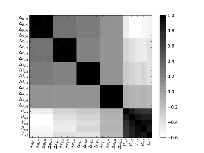
Finally, there is a last set of (systematic) uncertainties, which affects only the calibrated fluxes derived from the tertiary standard magnitudes: the errors related to the measurement of the SED of BD +17 4708, including the repeatability of the STIS measurements, and the absolute calibration of the STIS instrument. These uncertainties are discussed in §12. The associated covariance matrix is reported in table 21.

Table 21: Covariance matrix of the uncertainties affecting the synthetic instrumental magnitudes of BD +17 4708.

$${\mathbf{V}}_{SED_{BD+17}}=10^{-6}\times\begin{pmatrix}5.2760&1.1170&-2.0222&-6.1807&6.2336&6.0589&3.2774&0.6793&-3.2182\\ &8.9793&7.8773&9.9974&2.3035&1.7390&3.6392&8.9824&8.3187\\ &&14.2570&23.3526&-3.5755&-2.5778&1.7173&8.8588&16.9508\\ &&&46.0064&-9.7314&-7.8124&0.5591&11.9371&29.7526\\ &&&&11.0517&8.4008&3.6545&1.4931&-5.4785\\ &&&&&7.5107&3.6710&1.1458&-4.1358\\ &&&&&&3.2572&3.4286&1.3518\\ &&&&&&&9.1231&9.6018\\ &&&&&&&&20.7291\\ \end{pmatrix}\ \ \ \ \ \ \begin{matrix}g_{ref}\\ r_{ref}\\ i_{ref}\\ z_{ref}\\ U_{ref}\\ B_{ref}\\ V_{ref}\\ R_{ref}\\ I_{ref}\\ \end{matrix}$$

Appendix E Tertiary Catalogs

The tertiary catalogs built for the SNLS fields D1, D2, D3 and D4 are listed in tables LABEL:tab:d1_tertiaries, LABEL:tab:d2_tertiaries, LABEL:tab:d3_tertiaries and LABEL:tab:d4_tertiaries respectively.

They include the $u_{M}$ band calibrated magnitudes, derived as discussed in the previous section. For each star, we report the Local Natural Magnitudes, along with the $\delta k({\mathbf{x}})$ grid coefficient at the focal plane position where the star was observed. The Uniform Magnitudes can then be derived using the approximate formulas:

$$u_{|{\mathbf{x}}_{0}} = u_{|{\mathbf{x}}}-\delta k_{uug}({\mathbf{x}})\times(u_{|{\mathbf{x}}}-g_{|{\mathbf{x}}})$$

$$g_{|{\mathbf{x}}_{0}} = g_{|{\mathbf{x}}}-\delta k_{ggr}({\mathbf{x}})\times(g_{|{\mathbf{x}}}-r_{|{\mathbf{x}}})$$

$$r_{|{\mathbf{x}}_{0}} = r_{|{\mathbf{x}}}-\delta k_{rri}({\mathbf{x}})\times(r_{|{\mathbf{x}}}-i_{|{\mathbf{x}}})$$

$$i_{|{\mathbf{x}}_{0}} = i_{|{\mathbf{x}}}-\delta k_{iri}({\mathbf{x}})\times(r_{|{\mathbf{x}}}-i_{|{\mathbf{x}}})$$

$$z_{|{\mathbf{x}}_{0}} = z_{|{\mathbf{x}}}-\delta k_{ziz}({\mathbf{x}})\times(z_{|{\mathbf{x}}}-i_{|{\mathbf{x}}})$$ (32)

Indeed, the error resulting from using the local color: $\delta k({\mathbf{x}})\times{\rm col}_{|{\mathbf{x}}}$ instead of the color at the focal plane reference location: $\delta k(x)\times{\rm col}_{|{\mathbf{x}}_{0}}$, as requested by the grid definition, is smaller than 0.001 mag.

19

Table 22: Tertiary catalog for the SNLS field D1.

RA	DEC	$g_{M}$	$\sigma_{g_{M}}$	$N_{g_{M}}$	$\delta k_{ggr}$	$r_{M}$	$\sigma_{r_{M}}$	$N_{r_{M}}$	$\delta k_{rri}$	$i_{M}$	$\sigma_{i_{M}}$	$N_{i_{M}}$	$\delta k_{iri}$	$z_{M}$	$\sigma_{z_{M}}$	$N_{z_{M}}$	$\delta k_{ziz}$
(J2000)	(J2000)
$35.99905$	$-4.30274$	$20.282$	$0.009$	$3$	$0.033$	$18.768$	$0.005$	$6$	$0.037$	$17.716$	$0.005$	$7$	$0.024$	$17.263$	$0.011$	$3$	$0.053$
$36.00073$	$-4.44487$	$20.086$	$0.003$	$19$	$0.029$	$18.640$	$0.003$	$23$	$0.033$	$17.483$	$0.002$	$22$	$0.019$	$16.974$	$0.005$	$17$	$0.043$
$36.00134$	$-4.61800$	$17.520$	$0.003$	$17$	$0.021$	$16.727$	$0.003$	$16$	$0.032$	$16.312$	$0.005$	$5$	$0.020$	$16.124$	$0.005$	$14$	$0.034$
$36.00196$	$-4.26749$	–	–	–	–	$20.921$	$0.010$	$15$	$0.037$	$20.483$	$0.008$	$20$	$0.024$	–	–	–	–
$36.00311$	$-4.16810$	$20.873$	$0.004$	$25$	$0.029$	$20.122$	$0.004$	$22$	$0.043$	$19.706$	$0.004$	$30$	$0.041$	–	–	–	–
$36.00338$	$-4.45709$	$20.845$	$0.004$	$26$	$0.029$	$19.361$	$0.003$	$29$	$0.033$	$18.399$	$0.002$	$33$	$0.019$	$17.976$	$0.005$	$19$	$0.043$
$36.00416$	$-4.00506$	$20.662$	$0.008$	$5$	$0.040$	$19.356$	$0.004$	$10$	$0.040$	$18.657$	$0.003$	$15$	$0.050$	$18.292$	$0.006$	$18$	$0.037$
$36.00428$	$-4.65547$	$18.647$	$0.003$	$21$	$0.021$	$18.066$	$0.002$	$28$	$0.032$	$17.719$	$0.002$	$28$	$0.020$	$17.540$	$0.004$	$19$	$0.034$
$36.00460$	$-4.85283$	$19.996$	$0.003$	$23$	$0.025$	$19.556$	$0.003$	$29$	$0.044$	$19.267$	$0.003$	$31$	$0.039$	–	–	–	–
$36.00562$	$-4.42695$	–	–	–	–	$20.583$	$0.004$	$31$	$0.033$	$19.343$	$0.002$	$34$	$0.019$	$18.817$	$0.006$	$19$	$0.043$
$36.00588$	$-4.81196$	$20.736$	$0.004$	$23$	$0.024$	$19.257$	$0.002$	$29$	$0.041$	$17.770$	$0.002$	$32$	$0.034$	$17.107$	$0.004$	$19$	$0.043$
$36.00604$	$-4.07668$	–	–	–	–	$19.870$	$0.003$	$29$	$0.040$	$18.397$	$0.002$	$32$	$0.048$	$17.717$	$0.004$	$19$	$0.042$
$36.00673$	$-4.77046$	$20.013$	$0.003$	$26$	$0.024$	$19.509$	$0.003$	$29$	$0.041$	$19.229$	$0.002$	$34$	$0.034$	–	–	–	–
$36.00686$	$-4.27621$	$19.126$	$0.002$	$27$	$0.033$	$18.310$	$0.002$	$29$	$0.037$	$17.818$	$0.002$	$34$	$0.024$	$17.599$	$0.004$	$19$	$0.053$
$36.00716$	$-4.53652$	$18.682$	$0.002$	$27$	$0.020$	$17.831$	$0.002$	$24$	$0.024$	$17.397$	$0.002$	$29$	$0.021$	$17.187$	$0.004$	$18$	$0.028$
$36.00852$	$-4.96286$	–	–	–	–	–	–	–	–	$20.346$	$0.005$	$32$	$0.042$	–	–	–	–
$36.00870$	$-4.32838$	$20.176$	$0.003$	$28$	$0.033$	$18.770$	$0.002$	$32$	$0.037$	$17.700$	$0.002$	$35$	$0.024$	$17.251$	$0.004$	$19$	$0.053$
$36.00882$	$-4.41460$	–	–	–	–	–	–	–	–	$20.204$	$0.003$	$34$	$0.024$	–	–	–	–
$36.00887$	$-4.80380$	–	–	–	–	$20.871$	$0.004$	$31$	$0.041$	$20.660$	$0.005$	$33$	$0.034$	–	–	–	–
$36.00898$	$-4.54691$	$18.720$	$0.002$	$28$	$0.020$	$17.312$	$0.002$	$32$	$0.024$	$16.325$	$0.003$	$16$	$0.021$	$15.868$	$0.004$	$16$	$0.028$
$36.00898$	$-4.97885$	–	–	–	–	$20.983$	$0.006$	$25$	$0.040$	$19.822$	$0.004$	$32$	$0.042$	–	–	–	–
$36.00906$	$-4.87077$	–	–	–	–	–	–	–	–	$19.991$	$0.003$	$34$	$0.039$	–	–	–	–
$36.00914$	$-4.56453$	–	–	–	–	$20.394$	$0.003$	$32$	$0.024$	$18.824$	$0.002$	$35$	$0.021$	$18.135$	$0.004$	$19$	$0.028$
$36.00947$	$-4.05131$	–	–	–	–	–	–	–	–	$19.738$	$0.003$	$35$	$0.050$	–	–	–	–
$36.01037$	$-4.09691$	$17.649$	$0.002$	$27$	$0.033$	$16.753$	$0.002$	$27$	$0.040$	$16.270$	$0.003$	$11$	$0.048$	$16.018$	$0.004$	$18$	$0.042$
$36.01078$	$-4.60296$	–	–	–	–	–	–	–	–	$20.328$	$0.003$	$35$	$0.020$	–	–	–	–
$36.01084$	$-4.01824$	$17.405$	$0.002$	$26$	$0.040$	$16.364$	$0.002$	$21$	$0.040$	$15.844$	$0.005$	$5$	$0.050$	$15.601$	$0.004$	$15$	$0.037$
$36.01106$	$-4.39612$	$19.801$	$0.002$	$27$	$0.034$	$18.398$	$0.002$	$32$	$0.035$	$17.334$	$0.002$	$36$	$0.024$	$16.885$	$0.004$	$19$	$0.049$
$36.01133$	$-4.17180$	$19.583$	$0.002$	$27$	$0.029$	$18.207$	$0.002$	$32$	$0.043$	$17.435$	$0.002$	$35$	$0.041$	$17.060$	$0.004$	$18$	$0.041$
$36.01161$	$-4.16873$	$18.587$	$0.002$	$27$	$0.029$	$17.464$	$0.002$	$32$	$0.043$	$16.863$	$0.002$	$33$	$0.041$	$16.565$	$0.004$	$19$	$0.041$
$36.01239$	$-4.74109$	–	–	–	–	$20.891$	$0.004$	$29$	$0.035$	$20.212$	$0.004$	$28$	$0.021$	–	–	–	–
$36.01324$	$-4.83961$	$17.036$	$0.003$	$24$	$0.025$	$16.306$	$0.002$	$19$	$0.044$	$15.899$	$0.005$	$4$	$0.039$	$15.719$	$0.004$	$16$	$0.034$
$36.01386$	$-4.79779$	–	–	–	–	–	–	–	–	$20.566$	$0.004$	$32$	$0.034$	–	–	–	–
$36.01520$	$-4.90408$	–	–	–	–	–	–	–	–	$20.887$	$0.005$	$31$	$0.039$	–	–	–	–
$36.01573$	$-4.94662$	$19.364$	$0.002$	$28$	$0.030$	$17.900$	$0.002$	$32$	$0.040$	$16.556$	$0.002$	$21$	$0.042$	$15.914$	$0.003$	$19$	$0.030$
$36.01626$	$-4.79657$	$19.247$	$0.002$	$28$	$0.024$	$18.490$	$0.002$	$32$	$0.041$	$18.055$	$0.002$	$35$	$0.034$	$17.843$	$0.004$	$19$	$0.043$
$36.01638$	$-4.38600$	–	–	–	–	$20.899$	$0.003$	$32$	$0.035$	$20.430$	$0.003$	$34$	$0.024$	–	–	–	–
…	…	…	…	…	…	…	…	…	…	…	…	…	…	…	…	…	…

20

Table 23: Tertiary catalog for the SNLS field D2.

RA	DEC	$g_{M}$	$\sigma_{g_{M}}$	$N_{g_{M}}$	$\delta k_{ggr}$	$r_{M}$	$\sigma_{r_{M}}$	$N_{r_{M}}$	$\delta k_{rri}$	$i_{M}$	$\sigma_{i_{M}}$	$N_{i_{M}}$	$\delta k_{iri}$	$z_{M}$	$\sigma_{z_{M}}$	$N_{z_{M}}$	$\delta k_{ziz}$
(J2000)	(J2000)
$149.62000$	$2.32533$	–	–	–	–	–	–	–	–	$19.279$	$0.005$	$12$	$0.024$	$18.541$	$0.013$	$7$	$0.049$
$149.62034$	$2.47045$	$20.461$	$0.007$	$7$	$0.029$	$20.018$	$0.006$	$9$	$0.043$	$19.753$	$0.007$	$10$	$0.041$	–	–	–	–
$149.62099$	$2.12191$	–	–	–	–	$19.902$	$0.005$	$14$	$0.024$	$18.885$	$0.004$	$15$	$0.021$	$18.428$	$0.011$	$8$	$0.034$
$149.62127$	$2.28208$	$20.950$	$0.006$	$13$	$0.034$	$19.544$	$0.003$	$21$	$0.035$	$18.108$	$0.003$	$20$	$0.019$	$17.509$	$0.007$	$9$	$0.043$
$149.62128$	$2.05220$	–	–	–	–	$20.943$	$0.009$	$14$	$0.032$	$19.227$	$0.004$	$14$	$0.020$	$18.485$	$0.012$	$7$	$0.034$
$149.62135$	$2.18374$	$18.549$	$0.004$	$9$	$0.020$	$17.867$	$0.003$	$18$	$0.024$	$17.464$	$0.003$	$16$	$0.021$	$17.347$	$0.007$	$8$	$0.028$
$149.62140$	$2.51753$	–	–	–	–	$20.898$	$0.008$	$14$	$0.043$	$19.744$	$0.005$	$15$	$0.041$	–	–	–	–
$149.62149$	$2.67409$	–	–	–	–	$20.668$	$0.007$	$14$	$0.040$	$20.041$	$0.007$	$14$	$0.050$	–	–	–	–
$149.62175$	$2.68895$	–	–	–	–	–	–	–	–	$20.835$	$0.012$	$9$	$0.050$	–	–	–	–
$149.62177$	$2.20355$	$18.592$	$0.004$	$11$	$0.029$	$18.000$	$0.003$	$17$	$0.033$	$17.642$	$0.003$	$18$	$0.019$	$17.531$	$0.006$	$9$	$0.028$
$149.62230$	$2.57420$	–	–	–	–	$20.297$	$0.005$	$19$	$0.040$	$19.631$	$0.004$	$18$	$0.048$	–	–	–	–
$149.62263$	$1.92858$	$19.642$	$0.005$	$9$	$0.024$	$18.292$	$0.003$	$15$	$0.041$	$17.462$	$0.003$	$14$	$0.034$	$17.085$	$0.007$	$8$	$0.043$
$149.62275$	$2.51222$	–	–	–	–	$20.832$	$0.008$	$16$	$0.043$	$18.985$	$0.003$	$21$	$0.041$	$18.223$	$0.007$	$10$	$0.041$
$149.62294$	$2.11823$	$17.441$	$0.003$	$13$	$0.021$	$16.822$	$0.003$	$17$	$0.032$	$16.465$	$0.004$	$8$	$0.020$	$16.305$	$0.006$	$9$	$0.034$
$149.62313$	$2.40304$	$18.341$	$0.004$	$13$	$0.033$	$17.832$	$0.003$	$19$	$0.037$	–	–	–	–	$17.417$	$0.016$	$2$	$0.053$
$149.62320$	$2.50133$	$20.344$	$0.005$	$10$	$0.029$	$19.667$	$0.004$	$18$	$0.043$	$19.234$	$0.003$	$22$	$0.041$	–	–	–	–
$149.62353$	$2.50588$	–	–	–	–	$20.410$	$0.006$	$16$	$0.043$	$19.174$	$0.003$	$21$	$0.041$	$18.641$	$0.008$	$10$	$0.041$
$149.62382$	$2.64884$	$18.973$	$0.004$	$12$	$0.040$	$17.916$	$0.003$	$21$	$0.040$	$17.353$	$0.003$	$18$	$0.050$	$17.090$	$0.006$	$8$	$0.037$
$149.62427$	$2.34592$	–	–	–	–	–	–	–	–	$20.848$	$0.007$	$20$	$0.024$	–	–	–	–
$149.62444$	$2.16455$	–	–	–	–	–	–	–	–	$20.803$	$0.007$	$21$	$0.021$	–	–	–	–
$149.62516$	$2.13512$	$17.438$	$0.003$	$13$	$0.020$	$16.817$	$0.003$	$18$	$0.024$	$16.478$	$0.004$	$10$	$0.021$	$16.320$	$0.005$	$10$	$0.028$
$149.62525$	$2.17352$	$20.459$	$0.005$	$12$	$0.020$	$19.001$	$0.003$	$21$	$0.024$	$17.972$	$0.002$	$23$	$0.021$	$17.539$	$0.006$	$10$	$0.028$
$149.62570$	$2.50842$	$20.549$	$0.005$	$12$	$0.029$	$20.088$	$0.004$	$19$	$0.043$	$19.771$	$0.004$	$21$	$0.041$	–	–	–	–
$149.62603$	$2.44159$	–	–	–	–	–	–	–	–	$20.360$	$0.005$	$21$	$0.024$	–	–	–	–
$149.62679$	$1.83224$	$20.165$	$0.005$	$11$	$0.025$	$18.777$	$0.003$	$21$	$0.044$	$17.656$	$0.002$	$22$	$0.039$	$17.149$	$0.005$	$10$	$0.034$
$149.62693$	$2.67197$	–	–	–	–	$20.867$	$0.006$	$16$	$0.040$	$19.072$	$0.003$	$19$	$0.050$	$18.245$	$0.007$	$9$	$0.037$
$149.62720$	$2.43592$	–	–	–	–	$20.383$	$0.004$	$21$	$0.037$	$19.929$	$0.004$	$24$	$0.024$	–	–	–	–
$149.62724$	$2.00441$	$16.690$	$0.004$	$10$	$0.021$	$16.129$	$0.005$	$7$	$0.035$	$15.799$	$0.007$	$3$	$0.021$	$15.665$	$0.005$	$9$	$0.037$
$149.62735$	$2.66318$	–	–	–	–	–	–	–	–	$20.590$	$0.006$	$21$	$0.050$	–	–	–	–
$149.62741$	$1.79608$	$20.114$	$0.004$	$13$	$0.025$	$18.731$	$0.003$	$21$	$0.044$	$17.766$	$0.003$	$21$	$0.039$	$17.321$	$0.005$	$10$	$0.034$
$149.62757$	$2.49767$	$19.662$	$0.004$	$10$	$0.029$	$18.302$	$0.003$	$17$	$0.043$	$17.008$	$0.003$	$18$	$0.041$	$16.388$	$0.006$	$9$	$0.041$
$149.62773$	$1.86667$	–	–	–	–	$20.874$	$0.006$	$18$	$0.044$	$19.450$	$0.003$	$23$	$0.039$	$18.855$	$0.008$	$10$	$0.034$
$149.62796$	$2.67539$	–	–	–	–	–	–	–	–	$20.927$	$0.008$	$18$	$0.050$	–	–	–	–
$149.62824$	$1.91106$	$19.654$	$0.004$	$12$	$0.024$	$18.785$	$0.003$	$21$	$0.041$	$18.308$	$0.002$	$24$	$0.034$	$18.105$	$0.006$	$10$	$0.043$
$149.62848$	$1.73792$	$20.954$	$0.006$	$11$	$0.030$	$19.472$	$0.003$	$21$	$0.040$	$18.398$	$0.003$	$21$	$0.042$	$17.921$	$0.006$	$10$	$0.030$
$149.62865$	$2.51922$	$19.958$	$0.004$	$13$	$0.029$	$18.476$	$0.003$	$21$	$0.043$	$17.228$	$0.002$	$23$	$0.041$	$16.675$	$0.005$	$10$	$0.041$
$149.62915$	$2.64270$	$20.923$	$0.005$	$13$	$0.040$	$19.525$	$0.003$	$21$	$0.040$	$18.742$	$0.003$	$25$	$0.050$	$18.387$	$0.007$	$10$	$0.037$
…	…	…	…	…	…	…	…	…	…	…	…	…	…	…	…	…	…

21

Table 24: Tertiary catalog for the SNLS field D3.

RA	DEC	$g_{M}$	$\sigma_{g_{M}}$	$N_{g_{M}}$	$\delta k_{ggr}$	$r_{M}$	$\sigma_{r_{M}}$	$N_{r_{M}}$	$\delta k_{rri}$	$i_{M}$	$\sigma_{i_{M}}$	$N_{i_{M}}$	$\delta k_{iri}$	$z_{M}$	$\sigma_{z_{M}}$	$N_{z_{M}}$	$\delta k_{ziz}$
(J2000)	(J2000)
$214.04057$	$53.08957$	–	–	–	–	–	–	–	–	$20.073$	$0.005$	$30$	$0.048$	–	–	–	–
$214.04316$	$52.79265$	$20.378$	$0.004$	$19$	$0.034$	$18.946$	$0.002$	$28$	$0.035$	$17.279$	$0.002$	$29$	$0.024$	$16.593$	$0.006$	$8$	$0.049$
$214.04573$	$52.83204$	$19.926$	$0.003$	$27$	$0.034$	$18.673$	$0.002$	$32$	$0.035$	$17.985$	$0.002$	$39$	$0.024$	$17.677$	$0.007$	$10$	$0.049$
$214.04591$	$53.05735$	–	–	–	–	$20.777$	$0.004$	$31$	$0.040$	$20.161$	$0.004$	$35$	$0.048$	–	–	–	–
$214.04705$	$52.63229$	–	–	–	–	$20.749$	$0.005$	$28$	$0.024$	$19.037$	$0.003$	$32$	$0.021$	$18.310$	$0.009$	$9$	$0.028$
$214.04802$	$52.66266$	$17.936$	$0.003$	$25$	$0.020$	$16.498$	$0.003$	$15$	$0.024$	–	–	–	–	$15.027$	$0.008$	$4$	$0.028$
$214.04907$	$52.59444$	$20.944$	$0.004$	$25$	$0.020$	$19.554$	$0.003$	$29$	$0.024$	$18.505$	$0.002$	$34$	$0.020$	$18.030$	$0.007$	$10$	$0.034$
$214.04999$	$52.47645$	$18.327$	$0.004$	$14$	$0.021$	$17.435$	$0.003$	$21$	$0.035$	$16.947$	$0.003$	$18$	$0.021$	$16.714$	$0.007$	$8$	$0.037$
$214.05001$	$53.17555$	$20.731$	$0.004$	$16$	$0.040$	$20.247$	$0.004$	$17$	$0.040$	$19.964$	$0.005$	$27$	$0.050$	–	–	–	–
$214.05245$	$52.27888$	–	–	–	–	$17.808$	$0.004$	$7$	$0.044$	$16.947$	$0.004$	$8$	$0.039$	$16.541$	$0.009$	$4$	$0.034$
$214.05296$	$52.83856$	–	–	–	–	$20.885$	$0.003$	$33$	$0.035$	$19.240$	$0.002$	$39$	$0.024$	$18.604$	$0.008$	$10$	$0.049$
$214.05366$	$53.04250$	$17.383$	$0.003$	$25$	$0.033$	$15.995$	$0.004$	$10$	$0.040$	–	–	–	–	$14.824$	$0.010$	$3$	$0.042$
$214.05610$	$53.12693$	–	–	–	–	$20.476$	$0.003$	$34$	$0.040$	$19.918$	$0.003$	$39$	$0.050$	–	–	–	–
$214.05647$	$52.36586$	–	–	–	–	–	–	–	–	$20.635$	$0.007$	$29$	$0.034$	–	–	–	–
$214.05660$	$52.68815$	$17.613$	$0.002$	$27$	$0.029$	$17.017$	$0.002$	$34$	$0.033$	$16.667$	$0.002$	$28$	$0.019$	$16.524$	$0.005$	$10$	$0.043$
$214.05815$	$52.41449$	$19.833$	$0.008$	$3$	$0.024$	$19.148$	$0.004$	$10$	$0.041$	$18.760$	$0.003$	$24$	$0.034$	$18.572$	$0.010$	$8$	$0.043$
$214.05909$	$53.10057$	$18.543$	$0.002$	$28$	$0.040$	$18.069$	$0.002$	$34$	$0.040$	$17.790$	$0.002$	$39$	$0.050$	$17.664$	$0.006$	$10$	$0.037$
$214.05940$	$52.22233$	$18.895$	$0.004$	$13$	$0.030$	$17.517$	$0.003$	$16$	$0.040$	$16.711$	$0.003$	$11$	$0.042$	$16.323$	$0.006$	$8$	$0.030$
$214.05970$	$52.91299$	$19.717$	$0.003$	$28$	$0.033$	$18.259$	$0.002$	$31$	$0.037$	$16.948$	$0.002$	$35$	$0.024$	$16.382$	$0.005$	$10$	$0.053$
$214.05972$	$52.66918$	–	–	–	–	$20.921$	$0.003$	$34$	$0.024$	$19.399$	$0.002$	$39$	$0.021$	$18.794$	$0.008$	$10$	$0.028$
$214.06035$	$52.53434$	–	–	–	–	$20.948$	$0.004$	$34$	$0.032$	$19.155$	$0.002$	$39$	$0.020$	$18.365$	$0.007$	$10$	$0.034$
$214.06214$	$52.63167$	$20.342$	$0.003$	$28$	$0.020$	$18.985$	$0.002$	$34$	$0.024$	$17.480$	$0.002$	$39$	$0.021$	$16.827$	$0.005$	$10$	$0.028$
$214.06233$	$52.39881$	–	–	–	–	–	–	–	–	$20.400$	$0.004$	$38$	$0.034$	–	–	–	–
$214.06299$	$52.80484$	$18.096$	$0.002$	$28$	$0.034$	$17.526$	$0.002$	$34$	$0.035$	$17.185$	$0.002$	$37$	$0.024$	$17.044$	$0.005$	$10$	$0.049$
$214.06355$	$52.48590$	–	–	–	–	$19.753$	$0.002$	$33$	$0.035$	$18.366$	$0.002$	$39$	$0.021$	$17.755$	$0.006$	$10$	$0.037$
$214.06365$	$52.44070$	–	–	–	–	–	–	–	–	$20.976$	$0.007$	$32$	$0.021$	–	–	–	–
$214.06534$	$52.51261$	$19.890$	$0.003$	$28$	$0.021$	$18.477$	$0.002$	$34$	$0.035$	$17.470$	$0.002$	$39$	$0.021$	$16.996$	$0.005$	$10$	$0.037$
$214.06552$	$52.33159$	–	–	–	–	–	–	–	–	$20.095$	$0.003$	$39$	$0.039$	–	–	–	–
$214.06559$	$52.31804$	$17.934$	$0.002$	$28$	$0.025$	$17.156$	$0.002$	$34$	$0.044$	$16.696$	$0.002$	$31$	$0.039$	$16.464$	$0.005$	$10$	$0.034$
$214.06638$	$52.55993$	$20.364$	$0.003$	$28$	$0.021$	$18.905$	$0.002$	$34$	$0.032$	$17.751$	$0.002$	$39$	$0.020$	$17.220$	$0.005$	$10$	$0.034$
$214.06685$	$52.30431$	–	–	–	–	$19.681$	$0.002$	$33$	$0.044$	$18.612$	$0.002$	$39$	$0.039$	$18.100$	$0.006$	$10$	$0.034$
$214.06686$	$53.11036$	–	–	–	–	–	–	–	–	$20.936$	$0.005$	$39$	$0.050$	–	–	–	–
$214.06701$	$52.63149$	$20.834$	$0.003$	$28$	$0.020$	$19.408$	$0.002$	$34$	$0.024$	$18.093$	$0.002$	$39$	$0.021$	$17.508$	$0.006$	$10$	$0.028$
$214.06710$	$52.59462$	$17.697$	$0.002$	$27$	$0.021$	$16.940$	$0.002$	$33$	$0.032$	$16.522$	$0.002$	$22$	$0.021$	$16.308$	$0.005$	$10$	$0.034$
$214.06754$	$52.89887$	$19.008$	$0.002$	$28$	$0.033$	$18.300$	$0.002$	$32$	$0.037$	$17.905$	$0.002$	$38$	$0.024$	$17.749$	$0.007$	$8$	$0.053$
$214.06777$	$53.05638$	–	–	–	–	–	–	–	–	$20.478$	$0.004$	$39$	$0.048$	–	–	–	–
$214.06783$	$52.32591$	–	–	–	–	$20.036$	$0.002$	$34$	$0.044$	$19.287$	$0.002$	$39$	$0.039$	$18.921$	$0.009$	$9$	$0.034$
…	…	…	…	…	…	…	…	…	…	…	…	…	…	…	…	…	…

22

Table 25: Tertiary catalog for the SNLS field D4.

RA	DEC	$g_{M}$	$\sigma_{g_{M}}$	$N_{g_{M}}$	$\delta k_{ggr}$	$r_{M}$	$\sigma_{r_{M}}$	$N_{r_{M}}$	$\delta k_{rri}$	$i_{M}$	$\sigma_{i_{M}}$	$N_{i_{M}}$	$\delta k_{iri}$	$z_{M}$	$\sigma_{z_{M}}$	$N_{z_{M}}$	$\delta k_{ziz}$
(J2000)	(J2000)
$333.35788$	$-17.79348$	–	–	–	–	$20.685$	$0.009$	$14$	$0.024$	$19.508$	$0.006$	$18$	$0.021$	$18.979$	$0.015$	$10$	$0.028$
$333.35796$	$-17.84145$	–	–	–	–	$20.541$	$0.009$	$11$	$0.032$	$20.123$	$0.009$	$14$	$0.020$	–	–	–	–
$333.35919$	$-17.64129$	–	–	–	–	$19.762$	$0.003$	$31$	$0.035$	$18.954$	$0.003$	$26$	$0.024$	$18.648$	$0.009$	$16$	$0.049$
$333.35945$	$-17.58542$	–	–	–	–	–	–	–	–	$20.406$	$0.007$	$23$	$0.024$	–	–	–	–
$333.35955$	$-17.45383$	–	–	–	–	–	–	–	–	$20.456$	$0.010$	$17$	$0.041$	–	–	–	–
$333.35968$	$-17.52410$	–	–	–	–	$20.662$	$0.006$	$30$	$0.037$	$20.179$	$0.006$	$23$	$0.024$	–	–	–	–
$333.35984$	$-17.39324$	$20.821$	$0.004$	$28$	$0.033$	$19.977$	$0.004$	$27$	$0.040$	$19.466$	$0.005$	$24$	$0.048$	–	–	–	–
$333.36014$	$-17.76888$	$17.215$	$0.002$	$28$	$0.020$	$16.382$	$0.003$	$13$	$0.024$	$15.938$	$0.006$	$3$	$0.021$	$15.737$	$0.004$	$15$	$0.028$
$333.36015$	$-18.06026$	–	–	–	–	–	–	–	–	$20.166$	$0.007$	$21$	$0.034$	–	–	–	–
$333.36124$	$-17.66393$	$19.921$	$0.003$	$29$	$0.029$	$18.450$	$0.002$	$28$	$0.033$	$17.234$	$0.002$	$28$	$0.019$	$16.704$	$0.004$	$16$	$0.043$
$333.36128$	$-17.38790$	$19.486$	$0.003$	$26$	$0.033$	$18.828$	$0.002$	$32$	$0.040$	$18.428$	$0.003$	$26$	$0.048$	$18.273$	$0.007$	$16$	$0.042$
$333.36139$	$-17.30919$	$19.850$	$0.003$	$26$	$0.040$	$19.126$	$0.003$	$28$	$0.040$	$18.737$	$0.003$	$25$	$0.050$	$18.567$	$0.008$	$16$	$0.037$
$333.36183$	$-17.76437$	$17.665$	$0.002$	$28$	$0.020$	$17.086$	$0.002$	$29$	$0.024$	$16.776$	$0.002$	$22$	$0.021$	$16.649$	$0.004$	$17$	$0.028$
$333.36198$	$-18.15114$	$20.146$	$0.003$	$22$	$0.025$	$19.971$	$0.004$	$23$	$0.044$	$19.892$	$0.005$	$23$	$0.042$	–	–	–	–
$333.36212$	$-17.52031$	–	–	–	–	–	–	–	–	$20.728$	$0.008$	$20$	$0.024$	–	–	–	–
$333.36233$	$-17.63395$	$17.770$	$0.002$	$29$	$0.034$	$16.802$	$0.002$	$33$	$0.035$	$16.309$	$0.003$	$16$	$0.024$	$16.097$	$0.004$	$19$	$0.049$
$333.36247$	$-17.26413$	–	–	–	–	$20.044$	$0.004$	$28$	$0.040$	$18.830$	$0.003$	$28$	$0.050$	$18.273$	$0.007$	$16$	$0.037$
$333.36252$	$-17.69630$	$20.351$	$0.003$	$29$	$0.029$	$19.056$	$0.002$	$34$	$0.033$	$18.344$	$0.002$	$29$	$0.019$	$18.028$	$0.005$	$18$	$0.043$
$333.36290$	$-17.68844$	$19.345$	$0.002$	$30$	$0.029$	$17.842$	$0.002$	$33$	$0.033$	$16.563$	$0.002$	$22$	$0.019$	$16.033$	$0.004$	$18$	$0.043$
$333.36309$	$-17.75397$	$19.149$	$0.002$	$29$	$0.020$	$18.453$	$0.002$	$34$	$0.024$	$18.079$	$0.002$	$29$	$0.021$	$17.912$	$0.005$	$19$	$0.028$
$333.36337$	$-17.84771$	–	–	–	–	$20.525$	$0.004$	$33$	$0.032$	$20.149$	$0.005$	$28$	$0.020$	–	–	–	–
$333.36352$	$-18.03406$	–	–	–	–	$20.913$	$0.006$	$28$	$0.041$	$19.717$	$0.004$	$29$	$0.034$	–	–	–	–
$333.36386$	$-18.14651$	$20.709$	$0.004$	$24$	$0.025$	$19.197$	$0.003$	$29$	$0.044$	$17.800$	$0.002$	$27$	$0.042$	$17.157$	$0.005$	$14$	$0.034$
$333.36395$	$-17.43115$	–	–	–	–	–	–	–	–	$19.502$	$0.004$	$27$	$0.041$	$18.721$	$0.008$	$16$	$0.041$
$333.36439$	$-18.02007$	–	–	–	–	$20.318$	$0.004$	$30$	$0.041$	$19.057$	$0.003$	$29$	$0.034$	$18.484$	$0.006$	$17$	$0.043$
$333.36442$	$-17.45408$	–	–	–	–	–	–	–	–	$20.022$	$0.006$	$20$	$0.041$	–	–	–	–
$333.36459$	$-17.21264$	$18.992$	$0.004$	$10$	$0.040$	$17.581$	$0.003$	$13$	$0.040$	$16.582$	$0.004$	$8$	$0.050$	$16.100$	$0.010$	$4$	$0.037$
$333.36467$	$-17.54705$	$20.560$	$0.003$	$30$	$0.033$	$19.276$	$0.002$	$34$	$0.037$	$18.598$	$0.002$	$29$	$0.024$	$18.300$	$0.006$	$18$	$0.053$
$333.36483$	$-18.15027$	–	–	–	–	–	–	–	–	$20.736$	$0.008$	$21$	$0.042$	–	–	–	–
$333.36490$	$-18.03335$	–	–	–	–	–	–	–	–	$20.708$	$0.007$	$25$	$0.034$	–	–	–	–
$333.36497$	$-17.41420$	–	–	–	–	–	–	–	–	$20.862$	$0.009$	$18$	$0.041$	–	–	–	–
$333.36550$	$-17.51455$	$19.162$	$0.002$	$30$	$0.033$	$18.401$	$0.002$	$34$	$0.037$	$17.962$	$0.002$	$29$	$0.024$	$17.773$	$0.005$	$19$	$0.053$
$333.36579$	$-17.95646$	–	–	–	–	–	–	–	–	$20.198$	$0.005$	$27$	$0.021$	–	–	–	–
$333.36613$	$-17.77279$	$17.218$	$0.002$	$29$	$0.020$	$16.556$	$0.002$	$27$	$0.024$	$16.205$	$0.003$	$10$	$0.021$	$16.045$	$0.004$	$19$	$0.028$
$333.36655$	$-17.51977$	$20.637$	$0.003$	$30$	$0.033$	$19.208$	$0.002$	$34$	$0.037$	$17.913$	$0.002$	$29$	$0.024$	$17.375$	$0.004$	$19$	$0.053$
$333.36671$	$-17.89921$	$19.272$	$0.002$	$30$	$0.021$	$18.311$	$0.002$	$34$	$0.035$	$17.827$	$0.002$	$29$	$0.021$	$17.578$	$0.004$	$19$	$0.037$
$333.36710$	$-17.47462$	$17.946$	$0.002$	$27$	$0.029$	$17.193$	$0.002$	$31$	$0.043$	$16.767$	$0.002$	$23$	$0.024$	$16.558$	$0.004$	$16$	$0.041$
…	…	…	…	…	…	…	…	…	…	…	…	…	…	…	…	…	…

Appendix F Calibration of the $u_{M}$-band Data

The DEEP survey $u_{M}$-band data have also been analyzed. This calibration is less robust however, given the difficulties inherent to the calibration of near-UV data, and also given the small number of $u_{M}$-band epochs. Indeed, the $u_{M}$-band dataset not being formally part of the SNLS dataset, and the exposures are not time sequenced. In this section, we list the main results obtained on the $u_{M}$-band data.

The uniformity studies described in §6 have also been performed on the $u_{M}$-band data. Figure 22 presents one of the $\delta zp({\mathbf{x}})$ and $\delta k({\mathbf{x}})$ maps obtained in semester 2005B. We note that the $u_{M}$-band filter seems to be much more uniform than the other band filters. Also there seem to be sharp passband variations between the various CCDs. This is due to the fact that the blue edge of the MegaCam $u_{M}$-band is determined by the CCD quantum efficiencies.

 

(a) $\delta zp_{u,u-g}({\mathbf{x}})$

(b) $\delta k_{u,u-g}({\mathbf{x}})$

Figure 22: $u_{M}$-band grid maps. As can be seen, the $u_{M}$ filter seems more uniform than the other band filters. Sharp variations can be observed in the $\delta k({\mathbf{x}})$ maps. This is due to the fact that the blue edge of the $u_{M}$-filter is determined by the quantum efficiency of each CCD. Hence, the passband variations.

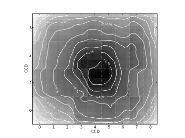
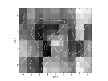
The $u_{M}$-band Landolt observations have been analyzed with the same procedure as the one described in this paper. The Landolt-to-MegaCam color transformations were modeled using a piecewise-linear function, with a break at $(U-B)_{0}\sim 0.4$:

$$u_{ADU|{\mathbf{x}}_{0}} = U-k_{u}\times(X-1) + \alpha_{u}\times(U-B)$$

$${\rm if\ U-B<(U-B)_{0}}$$

$$u_{ADU|{\mathbf{x}}_{0}} = U-k_{u}\times(X-1) + \alpha_{u}\times(U-B)_{0}$$

$$+ \beta_{u}\times\left[(U-B)-(U-B)_{0}\right]$$

$${\rm if\ U-B>(U-B)_{0}}$$

We found:

$$\alpha_{u} = -0.2450\pm 0.0108$$

$$\beta_{u} = -0.2787\pm 0.0070$$

$$k_{u} = -0.0758\pm 0.0087$$ (33)

The zero-points determined along with the global parameters $\alpha_{u}$, $\beta_{u}$ and $k_{u}$ were applied to the tertiary instrumental magnitudes which where then averaged to give final calibrated magnitudes. Due to the smaller number of epochs, the night selection was much less robust. We just remove the “pathological nights” that display an absorption larger than 0.1 mag.

(a) $u_{M}-g_{M}\ vs.g_{M}-r_{M}$

(b) $u_{M}-g_{M}\ vs.g_{M}-r_{M}$ (profile)

Figure 23: Left: $u_{M}-g_{M}$ versus $g_{M}-r_{M}$ color-color plot of the tertiary standards. Right: a zoom on the $0.4<u_{M}-g_{M}<1.5$ region of the color-color plot, after subtraction of the mean slope. We see that the $u_{M}-g_{M}$ colors of the three D1, D2 and D3 fields agree within one percent. The origin of the systematic shift which affect the D4 colors is not clearly identified.

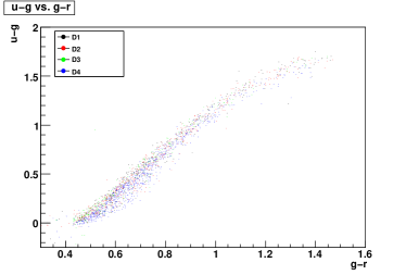
Figure 23 presents the $u_{M}-g_{M}$ versus $g_{M}-r_{M}$ color-color diagram for all four SNLS fields. As can be seen, the $u_{M}-g_{M}$ colors of the three D1, D2 and D3 fields agree within one percent. On the other hand, the stellar locus of the D4 field is about 4% away from that of the other fields. The reason for this is not clear yet. In particular, D4 is affected by the same Galactic absorption as, for exampled, D1 ($E(B-V)\sim 0.027$ for both). Note that we observe the same phenomenon –although much weaker– on the $r_{M}-i_{M}$ vs. $g_{M}-r_{M}$ diagram (figure 17).

The $u_{M}$-band magnitudes determined in this section can be retrieved in electronic form at the CDS. Aside from the main catalogs, described in the previous section, we have released similar catalogs containing the subset of tertiary standards with $u_{M}$-band magnitudes.

As for the main catalogs, we report the Local Natural Magnitudes of each star. The flux interpretation of those magnitudes relies on the MegaCam $u_{M}$-band magnitude of BD +17 4708, which can be derived as described in §10. Using the color transformations determine above, we can compute a first order estimate of the $u_{M}$-band magnitude of BD +17 4708:

$$u_{BD\leavevmode\nobreak\ +17\leavevmode\nobreak\ 4708}=9.7688\pm 0.0027\ +\Delta u_{M}$$

This estimate should be corrected by an offset $\Delta u$, which would account for the fact that the actual $u_{M}$-band magnitude of BD +17 4708 which would be observed by MegaCam does not necessarily follow exactly the linear Landolt-to-MegaCam color law. Such an offset may be computed using synthetic photometry of BD +17 4708 as described in §10. However, given the fact that we have not extensively tested the instrument and the Mauna Kea atmospheric extinction in the $u_{M}$-band, we prefer not to publish any number.

Clearly, the $u_{M}$-band calibration of the CFHTLS survey will be considerably improved by (1) adding more epochs and (2) observing a set of fundamental standards directly with MegaCam. This is the goal of the MAPC program, already discussed in this paper.

Appendix G MegaCam-to-SDSS Color Transformations

Two CFHTLS DEEP fields, D2 and D3 were also observed by the SDSS collaboration. While the intercalibration of the MegaCam and SDSS surveys deserves its own paper, it is possible to use the observations of D2 and D3 to derive the color transformations between the SDSS and MegaCam magnitudes. We used the SDSS DR6 catalogs and determined the color transformations between the SDSS and MegaCam transformations at the focal plane center. We found the color transformations to be linear, and equal to:

$$u_{|{\mathbf{x}}_{0}}-u_{SDSS} = -0.211(\pm 0.004)\times(u_{SDSS}-g_{SDSS})+{\Delta zp_{u}}$$

$$g_{|{\mathbf{x}}_{0}}-g_{SDSS} = -0.155(\pm 0.003)\times(g_{SDSS}-r_{SDSS})+{\Delta zp_{g}}$$

$$r_{|{\mathbf{x}}_{0}}-r_{SDSS} = -0.030(\pm 0.004)\times(r_{SDSS}-i_{SDSS})+{\Delta zp_{r}}$$

$$i_{|{\mathbf{x}}_{0}}-i_{SDSS} = -0.102(\pm 0.005)\times(r_{SDSS}-i_{SDSS})+{\Delta zp_{i}}$$

$$z_{|{\mathbf{x}}_{0}}-z_{SDSS} = +0.036(\pm 0.008)\times(i_{SDSS}-z_{SDSS})+{\Delta zp_{z}}$$ (34)

As one can expect, there are non-zero offsets between the SDSS 2.5-m and the SNLS system ($\Delta u\sim-0.56$, $\Delta g\sim+0.11$, $\Delta r\sim-0.14$, $\Delta i\sim-0.32$ and $\Delta z\sim-0.43$). The precise measurement of these offsets along with the associated uncertainties will be the subject of a later paper.