Searching for Galactic White Dwarf Binaries in Mock LISA Data using an $\mathcal{F}$-Statistic Template Bank

Abstract

We describe an $\mathcal{F}$-statistic search for continuous gravitational waves from galactic white-dwarf binaries in simulated LISA Data. Our search method employs a hierarchical template-grid based exploration of the parameter space. In the first stage, candidate sources are identified in searches using different simulated laser signal combinations (known as TDI variables). Since each source generates a primary maximum near its true “Doppler parameters” (intrinsic frequency and sky position) as well as numerous secondary maxima of the $\mathcal{F}$-statistic in Doppler parameter space, a search for multiple sources needs to distinguish between true signals and secondary maxima associated with other, “louder” signals. Our method does this by applying a coincidence test to reject candidates which are not found at nearby parameter space positions in searches using each of the three TDI variables. For signals surviving the coincidence test, we perform a fully coherent search over a refined parameter grid to provide an accurate parameter estimation for the final candidates. Suitably tuned, the pipeline is able to extract 1989 true signals with only 5 false alarms. The use of the rigid adiabatic approximation allows recovery of signal parameters with errors comparable to statistical expectations, although there is still some systematic excess with respect to statistical errors expected from Gaussian noise. An experimental iterative pipeline with seven rounds of signal subtraction and re-analysis of the residuals allows us to increase the number of signals recovered to a total of 3419 with 29 false alarms.

I Introduction

The Mock LISA Data Challenges (MLDCs) MLDC Task Force (a) have the purpose of encouraging the development of LISA data-analysis tools and assessing the technical readiness of the community to perform gravitational-wave (GW) astronomy with LISA. The rounds completed so far have been labelled MLDC1 Arnaud et al. (2007), MLDC2 Babak et al. (2008a), MLDC1B Babak et al. (2008b), and MLDC3 Babak et al. (2008b, 2009). The challenges have consisted of several data-sets containing different types of simulated sources and LISA noise, including quasi-periodic signals from white-dwarf binaries (WDBs). In this paper we describe an analysis performed on MLDC2 data, using an improved version of the pipeline that we originally applied in our MLDC2 entryBabak et al. (2008a); Prix and Whelan (2007a)

GW signals from WDBs will be long-lasting and (quasi-)monochromatic with slowly-varying intrinsic frequency $f(\tau)$; in this sense they belong to the class of continuous GWs. In the case of ground-based detectors the typical sources of continuous GWs are spinning neutron stars with non-axisymmetric deformations. One of the standard tools developed for these searches is the $\mathcal{F}$-statistic. We have applied this method in our MLDC searches, adapting the LAL/LALApps LIGO Scientific Collaboration search code ComputeFStatistic_v2 used within the LIGO Scientific Collaboration to search for periodic GW signals in data from ground-based detectors such as LIGO and GEO 600, e.g. see Wette et al. (2008).

MLDC1 and MLDC1B contained data sets with a relatively small number of simulated WDB signals, and the results of our searches on those data are reported elsewhere Prix and Whelan (2007b); Whelan et al. (2008). The MLDC2 data-set contains a full simulated galaxy of WDB signals, with the challenge being to extract as many of these signals as possible. One approach, used by Crowder et al Crowder and Cornish (2007b, a), is to fit the overall signal with a multi-source template. Our analysis instead applies the traditional method of searching for individual sources. An important challenge in that regard is to distinguish secondary maxima in parameter space from primary peaks of true signals. We accomplish this through a hierarchical pipeline, which follows up candidates found in coincidence between searches carried out with different LISA observables.

The plan for the rest of this paper is as follows: In section II we review the fundamentals of the $\mathcal{F}$-statistic search as applied to WDB signals in mock LISA data. In section III we describe our pipeline including the coincidence condition used to distinguish true signals from secondary maxima, and the estimation of expected statistical errors in the signal parameters. In section IV we describe some of the techniques used to evaluate the effectiveness of our pipeline: the post-hoc classification of candidates into found signals and false alarms, and the discrepancies between the candidate parameters returned by our pipeline and the simulated values. In section V we describe the results of our pipeline in its optimal configuration and compare those with the results obtained using less sophisticated models of the LISA response. In section VI we present the results of an iterative program in which the signals found by the pipeline are subtracted from the data stream and then the pipeline is re-run on the residuals.

II Search method for continuous signals from white-dwarf binaries

II.1 The $\mathcal{F}$-statistic

The $\mathcal{F}$-statistic was originally developed in Jaranowski et al. (1998), extended to the multi-detector case in Cutler and Schutz (2005), and generalized to the full Time-Domain Interferometry (TDI) Armstrong et al. (1999) framework for LISA in Krolak et al. (2004). The formalism for our application of this method to mock LISA data has been described in Prix and Whelan (2007b) and Whelan et al. (2008), to which the reader is referred for details. Here we review the fundamentals of the method relevant to the current application.

The signal received from a monochromatic GW source like a white-dwarf binary with negligible orbital evolution can be characterized by seven parameters. The three Doppler parameters are the intrinsic frequency $f$ and two coordinates describing the sky location, such as galactic latitude $\beta$ and longitude $\lambda$, and can be denoted as $\theta\equiv\{f,\beta,\lambda\}$. The four amplitude parameters are the overall GW amplitude $h_{0}$, the inclination angle $\iota$ of the orbital plane, the polarization angle $\psi$, and the initial phase $\phi_{0}$. One set of convenient combinations $\mathcal{A}^{\mu}=\mathcal{A}^{\mu}(h_{0},\iota,\psi,\phi_{0})$ is

$$\mathcal{A}^{1} =A_{+}\cos\phi_{0}\cos 2\psi-A_{\times}\sin\phi_{0}\sin 2\psi\,,$$ (1a)

$$\mathcal{A}^{2} =A_{+}\cos\phi_{0}\sin 2\psi+A_{\times}\sin\phi_{0}\cos 2\psi\,,$$ (1b)

$$\mathcal{A}^{3} =-A_{+}\sin\phi_{0}\cos 2\psi-A_{\times}\cos\phi_{0}\sin 2\psi\,,$$ (1c)

$$\mathcal{A}^{4} =-A_{+}\sin\phi_{0}\sin 2\psi+A_{\times}\cos\phi_{0}\cos 2\psi\,,$$ (1d)

where $A_{+}=h_{0}(1+\cos^{2}\iota)/2$ and $A_{\times}=h_{0}\cos\iota$. Using these combinations, it is possible to write the signal received in a detector $I$ with instrumental noise $n^{I}(t)$ as

$$x^{I}(t)=n^{I}(t)+\mathcal{A}^{\mu}\,h^{I}_{\mu}(t;\theta)\,,$$ (2)

where we introduce the convention of an implicit sum $\sum_{\mu=1}^{4}$ over repeated indices $\mu,\nu$, and the form of the template waveforms $h^{I}_{\mu}(t;\theta)$ depends on the Doppler parameters and the specifics of the detector, such as orientation and motion as a function of time.

Following the notation of Cutler and Schutz (2005); Prix (2007), we write the different data-streams $x^{I}(t)$ as a vector $\mathchoice{\mbox{\boldmath$\displaystyle x$}}{\mbox{\boldmath$\textstyle x$}}{\mbox{\boldmath$\scriptstyle x$}}{\mbox{\boldmath$\scriptscriptstyle x$}}(t)$, and we define the standard multi-detector (with uncorrelated noise) scalar product as

$$(\mathchoice{\mbox{\boldmath$\displaystyle x$}}{\mbox{\boldmath$\textstyle x$}}{\mbox{\boldmath$\scriptstyle x$}}{\mbox{\boldmath$\scriptscriptstyle x$}}|\mathchoice{\mbox{\boldmath$\displaystyle y$}}{\mbox{\boldmath$\textstyle y$}}{\mbox{\boldmath$\scriptstyle y$}}{\mbox{\boldmath$\scriptscriptstyle y$}})=\sum_{\alpha}\sum_{I}\int_{-\infty}^{\infty}\widetilde{x}_{\alpha}^{I*}(f)\,[S_{\alpha\,I}(f)]^{-1}\,\widetilde{y}_{\alpha}^{I}(f)\,df\,.$$ (3)

Here we have broken up the observation time into intervals labelled by $\alpha$, $\widetilde{x}_{\alpha}$ is the Fourier-transform of the data in the $\alpha$th time interval, $x^{*}$ denotes complex conjugation, and $\{S_{\alpha\,I}(f)\}$ is the two-sided noise power spectral density appropriate to the $\alpha$th time interval. We search for a signal $\{\mathcal{A}_{\mathrm{s}},\theta_{\mathrm{s}}\}$ by seeking the parameters $\{\mathcal{A}_{\mathrm{c}},\theta_{\mathrm{c}}\}$ which maximize the log-likelihood ratio

$$L(\mathchoice{\mbox{\boldmath$\displaystyle x$}}{\mbox{\boldmath$\textstyle x$}}{\mbox{\boldmath$\scriptstyle x$}}{\mbox{\boldmath$\scriptscriptstyle x$}};\mathcal{A},\theta)=(\mathchoice{\mbox{\boldmath$\displaystyle x$}}{\mbox{\boldmath$\textstyle x$}}{\mbox{\boldmath$\scriptstyle x$}}{\mbox{\boldmath$\scriptscriptstyle x$}}|\mathchoice{\mbox{\boldmath$\displaystyle h$}}{\mbox{\boldmath$\textstyle h$}}{\mbox{\boldmath$\scriptstyle h$}}{\mbox{\boldmath$\scriptscriptstyle h$}})-\frac{1}{2}(\mathchoice{\mbox{\boldmath$\displaystyle h$}}{\mbox{\boldmath$\textstyle h$}}{\mbox{\boldmath$\scriptstyle h$}}{\mbox{\boldmath$\scriptscriptstyle h$}}|\mathchoice{\mbox{\boldmath$\displaystyle h$}}{\mbox{\boldmath$\textstyle h$}}{\mbox{\boldmath$\scriptstyle h$}}{\mbox{\boldmath$\scriptscriptstyle h$}})=\mathcal{A}^{\mu}(\mathchoice{\mbox{\boldmath$\displaystyle x$}}{\mbox{\boldmath$\textstyle x$}}{\mbox{\boldmath$\scriptstyle x$}}{\mbox{\boldmath$\scriptscriptstyle x$}}|\mathchoice{\mbox{\boldmath$\displaystyle h$}}{\mbox{\boldmath$\textstyle h$}}{\mbox{\boldmath$\scriptstyle h$}}{\mbox{\boldmath$\scriptscriptstyle h$}}_{\mu})-\frac{1}{2}\mathcal{A}^{\mu}(\mathchoice{\mbox{\boldmath$\displaystyle h$}}{\mbox{\boldmath$\textstyle h$}}{\mbox{\boldmath$\scriptstyle h$}}{\mbox{\boldmath$\scriptscriptstyle h$}}_{\mu}|\mathchoice{\mbox{\boldmath$\displaystyle h$}}{\mbox{\boldmath$\textstyle h$}}{\mbox{\boldmath$\scriptstyle h$}}{\mbox{\boldmath$\scriptscriptstyle h$}}_{\nu})\mathcal{A}^{\nu}\,.$$ (4)

Defining

$$x_{\mu}(\theta)\equiv(\mathchoice{\mbox{\boldmath$\displaystyle x$}}{\mbox{\boldmath$\textstyle x$}}{\mbox{\boldmath$\scriptstyle x$}}{\mbox{\boldmath$\scriptscriptstyle x$}}|\mathchoice{\mbox{\boldmath$\displaystyle h$}}{\mbox{\boldmath$\textstyle h$}}{\mbox{\boldmath$\scriptstyle h$}}{\mbox{\boldmath$\scriptscriptstyle h$}}_{\mu})\,,\quad\mbox{and}\quad\mathcal{M}_{\mu\nu}(\theta)\equiv(\mathchoice{\mbox{\boldmath$\displaystyle h$}}{\mbox{\boldmath$\textstyle h$}}{\mbox{\boldmath$\scriptstyle h$}}{\mbox{\boldmath$\scriptscriptstyle h$}}_{\mu}|\mathchoice{\mbox{\boldmath$\displaystyle h$}}{\mbox{\boldmath$\textstyle h$}}{\mbox{\boldmath$\scriptstyle h$}}{\mbox{\boldmath$\scriptscriptstyle h$}}_{\nu})\,,$$ (5)

we see that $L$ is maximized for given $\theta$ by the amplitude estimator $\mathcal{A}_{{\mathrm{c}}}^{\mu}=\mathcal{M}^{\mu\nu}x_{\nu}$, where $\mathcal{M}^{\mu\nu}$ is the inverse matrix of $\mathcal{M}_{\mu\nu}$. Thus the detection statistic $L$, maximized over the amplitude parameters $\mathcal{A}$ is

$$2\mathcal{F}(\mathchoice{\mbox{\boldmath$\displaystyle x$}}{\mbox{\boldmath$\textstyle x$}}{\mbox{\boldmath$\scriptstyle x$}}{\mbox{\boldmath$\scriptscriptstyle x$}};\theta)\equiv\,x_{\mu}\,\mathcal{M}^{\mu\nu}\,x_{\nu}\,,$$ (6)

which defines the (multi-detector) $\mathcal{F}$-statistic. One can show that the expectation in the perfect-match case $\theta=\theta_{\mathrm{s}}$ is $E[2\mathcal{F}(\theta_{\mathrm{s}})]=4+\left\lvert\mathcal{A}_{\mathrm{s}}\right\rvert^{2}$, where we used the definition

$$\left\lvert\mathcal{A}\right\rvert^{2}\equiv\mathcal{A}^{\mu}\mathcal{M}_{\mu\nu}(\theta_{\mathrm{s}})\mathcal{A}^{\nu}\,,$$ (7)

for the norm of a 4-vector $\mathcal{A}^{\mu}$, using $\mathcal{M}_{\mu\nu}$ as a metric on the amplitude-parameter space. Note that $\left\lvert\mathcal{A}_{\mathrm{s}}\right\rvert$ is the (optimal) signal-to-noise ratio (SNR) of the true signal $\{\mathcal{A}_{\mathrm{s}},\theta_{\mathrm{s}}\}$.

II.2 Modelling the LISA response

The MLDC data were generated by two different programs: Synthetic LISA Vallisneri simulates a detector output consisting of Doppler shifts of the LISA lasers due to relative motion of the spacecraft, while LISA Simulator Cornish and Rubbo simulates the phase differences between laser light following different paths between the spacecraft. In both cases the underlying variables are combined with appropriate time shifts to form TDI observables which cancel the (otherwise dominating) laser frequency noise Armstrong et al. (1999); Tinto et al. (2004); Krolak et al. (2004). One choice of such TDI quantities is the set of three observables $\{X,Y,Z\}$. These observables, which can be thought of as representing the output of three virtual “detectors” (which we label with the index $I$), are related to the gravitational wave tensor ${\mathchoice{\mathord{\hbox to0.0pt{\hbox to8.79988pt{\hss$\displaystyle h$\hss}\hss}\raise 7.98605pt\hbox to8.79988pt{\hss\hbox{$\scriptstyle\leftrightarrow$}\hss}}}{\mathord{\hbox to0.0pt{\hbox to8.79988pt{\hss$\textstyle h$\hss}\hss}\raise 7.98605pt\hbox to8.79988pt{\hss\hbox{$\scriptstyle\leftrightarrow$}\hss}}}{\mathord{\hbox to0.0pt{\hbox to6.99988pt{\hss$\scriptstyle h$\hss}\hss}\raise 5.59023pt\hbox to6.99988pt{\hss\hbox{$\scriptscriptstyle\leftrightarrow$}\hss}}}{\mathord{\hbox to0.0pt{\hbox to6.99988pt{\hss$\scriptscriptstyle h$\hss}\hss}\raise 3.99301pt\hbox to6.99988pt{\hss\hbox{$\scriptscriptstyle\leftrightarrow$}\hss}}}}\mathord{}$ through the detector “response”, which can be modelled at different levels of accuracy. Our current approach uses the rigid adiabatic approximation Rubbo et al. (2004), but we also consider the long-wavelength limit (LWL). In the LWL approximation the reduced wavelength $c/(2\pi f)$ is assumed to be large compared to the distance $L$ between the spacecraft, which corresponds to a light-travel time of $T=L/c\sim 17\text{\,s}$ (assuming equal arm-lengths), and so this approximation requires $f\ll 10\text{\,mHz}$. These alternatives and their consequences are considered in more detail in Whelan et al. (2008), but here we summarize the relevant approximations as they apply to our search.

Figure 1: LISA configuration and TDI conventions used.

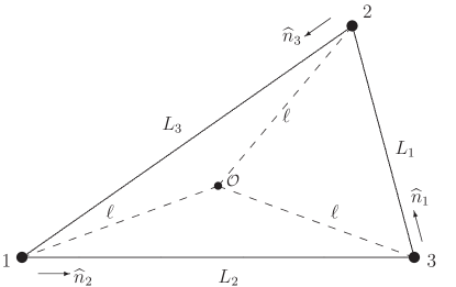
It is convenient to describe the “response” of a gravitational wave detector in the frequency domain in terms of a response function $R(f)$, relating the detector output to a “strain” more closely connected to the metric perturbation tensor ${\mathchoice{\mathord{\hbox to0.0pt{\hbox to8.79988pt{\hss$\displaystyle h$\hss}\hss}\raise 7.98605pt\hbox to8.79988pt{\hss\hbox{$\scriptstyle\leftrightarrow$}\hss}}}{\mathord{\hbox to0.0pt{\hbox to8.79988pt{\hss$\textstyle h$\hss}\hss}\raise 7.98605pt\hbox to8.79988pt{\hss\hbox{$\scriptstyle\leftrightarrow$}\hss}}}{\mathord{\hbox to0.0pt{\hbox to6.99988pt{\hss$\scriptstyle h$\hss}\hss}\raise 5.59023pt\hbox to6.99988pt{\hss\hbox{$\scriptscriptstyle\leftrightarrow$}\hss}}}{\mathord{\hbox to0.0pt{\hbox to6.99988pt{\hss$\scriptscriptstyle h$\hss}\hss}\raise 3.99301pt\hbox to6.99988pt{\hss\hbox{$\scriptscriptstyle\leftrightarrow$}\hss}}}}\mathord{}$, so that

$$\widetilde{X}(f)=\frac{\widetilde{h}^{X}(f)}{R(f)}=\frac{{\mathchoice{\mathord{\hbox to0.0pt{\hbox to8.79988pt{\hss$\displaystyle d$\hss}\hss}\raise 7.98605pt\hbox to8.79988pt{\hss\hbox{$\scriptstyle\leftrightarrow$}\hss}}}{\mathord{\hbox to0.0pt{\hbox to8.79988pt{\hss$\textstyle d$\hss}\hss}\raise 7.98605pt\hbox to8.79988pt{\hss\hbox{$\scriptstyle\leftrightarrow$}\hss}}}{\mathord{\hbox to0.0pt{\hbox to6.99988pt{\hss$\scriptstyle d$\hss}\hss}\raise 5.59023pt\hbox to6.99988pt{\hss\hbox{$\scriptscriptstyle\leftrightarrow$}\hss}}}{\mathord{\hbox to0.0pt{\hbox to6.99988pt{\hss$\scriptscriptstyle d$\hss}\hss}\raise 3.99301pt\hbox to6.99988pt{\hss\hbox{$\scriptscriptstyle\leftrightarrow$}\hss}}}}\mathord{}^{X}:\widetilde{{\mathchoice{\mathord{\hbox to0.0pt{\hbox to8.79988pt{\hss$\displaystyle h$\hss}\hss}\raise 7.98605pt\hbox to8.79988pt{\hss\hbox{$\scriptstyle\leftrightarrow$}\hss}}}{\mathord{\hbox to0.0pt{\hbox to8.79988pt{\hss$\textstyle h$\hss}\hss}\raise 7.98605pt\hbox to8.79988pt{\hss\hbox{$\scriptstyle\leftrightarrow$}\hss}}}{\mathord{\hbox to0.0pt{\hbox to6.99988pt{\hss$\scriptstyle h$\hss}\hss}\raise 5.59023pt\hbox to6.99988pt{\hss\hbox{$\scriptscriptstyle\leftrightarrow$}\hss}}}{\mathord{\hbox to0.0pt{\hbox to6.99988pt{\hss$\scriptscriptstyle h$\hss}\hss}\raise 3.99301pt\hbox to6.99988pt{\hss\hbox{$\scriptscriptstyle\leftrightarrow$}\hss}}}}\mathord{}}(f)}{R(f)}\,,$$ (8)

where $:$ denotes the contraction of both tensor indices. In the long-wavelength limit,

$$R^{\text{synthLISA}}(f)\approx R^{\text{synthLISA}}_{\text{LWL}}(f) =\left(\frac{1}{4\pi fT}\right)^{2}\,,$$ (9a)

$$R^{\text{LISAsim}}(f)\approx R^{\text{LISAsim}}_{\text{LWL}}(f) =i\frac{1}{4\pi fT}\,,$$ (9b)

and ${\mathchoice{\mathord{\hbox to0.0pt{\hbox to8.79988pt{\hss$\displaystyle d$\hss}\hss}\raise 7.98605pt\hbox to8.79988pt{\hss\hbox{$\scriptstyle\leftrightarrow$}\hss}}}{\mathord{\hbox to0.0pt{\hbox to8.79988pt{\hss$\textstyle d$\hss}\hss}\raise 7.98605pt\hbox to8.79988pt{\hss\hbox{$\scriptstyle\leftrightarrow$}\hss}}}{\mathord{\hbox to0.0pt{\hbox to6.99988pt{\hss$\scriptstyle d$\hss}\hss}\raise 5.59023pt\hbox to6.99988pt{\hss\hbox{$\scriptscriptstyle\leftrightarrow$}\hss}}}{\mathord{\hbox to0.0pt{\hbox to6.99988pt{\hss$\scriptscriptstyle d$\hss}\hss}\raise 3.99301pt\hbox to6.99988pt{\hss\hbox{$\scriptscriptstyle\leftrightarrow$}\hss}}}}\mathord{}^{X}\approx{\mathchoice{\mathord{\hbox to0.0pt{\hbox to8.79988pt{\hss$\displaystyle d$\hss}\hss}\raise 7.98605pt\hbox to8.79988pt{\hss\hbox{$\scriptstyle\leftrightarrow$}\hss}}}{\mathord{\hbox to0.0pt{\hbox to8.79988pt{\hss$\textstyle d$\hss}\hss}\raise 7.98605pt\hbox to8.79988pt{\hss\hbox{$\scriptstyle\leftrightarrow$}\hss}}}{\mathord{\hbox to0.0pt{\hbox to6.99988pt{\hss$\scriptstyle d$\hss}\hss}\raise 5.59023pt\hbox to6.99988pt{\hss\hbox{$\scriptscriptstyle\leftrightarrow$}\hss}}}{\mathord{\hbox to0.0pt{\hbox to6.99988pt{\hss$\scriptscriptstyle d$\hss}\hss}\raise 3.99301pt\hbox to6.99988pt{\hss\hbox{$\scriptscriptstyle\leftrightarrow$}\hss}}}}\mathord{}^{X}_{\text{LWL}}\equiv(\widehat{n}_{2}\otimes\widehat{n}_{2}-\widehat{n}_{3}\otimes\widehat{n}_{3})/2$ is the usual LWL response tensor for a GW interferometer with arms $\widehat{n}_{2}$ and $\widehat{n}_{3}$. The analogous expressions for $Y$ and $Z$ are obtained by cyclic permutations of the indices $1\rightarrow 2\rightarrow 3\rightarrow 1$. In the remainder of this section we will give explicit expressions associated with the $X$ variable, with the understanding that the formulas related to $Y$ and $Z$ can be constructed by analogy.

A more accurate approximation to the TDI response is the so-called rigid adiabatic (RA) approximation Rubbo et al. (2004), which is valid in the regime where the finite lengths of data used to approximate the idealized Fourier transforms are short enough that the geometry and orientation of the detector doesn’t change significantly during this time. In the RA formalism, the response is

$$R(f)=\frac{R_{\text{LWL}}(f)\,e^{i4\pi fT}}{\operatorname{sinc}\left({2\pi fT}\right)}\,,$$ (10)

and, for a wave propagating along the unit vector $\widehat{k}$,

$${\mathchoice{\mathord{\hbox to0.0pt{\hbox to8.79988pt{\hss$\displaystyle d$\hss}\hss}\raise 7.98605pt\hbox to8.79988pt{\hss\hbox{$\scriptstyle\leftrightarrow$}\hss}}}{\mathord{\hbox to0.0pt{\hbox to8.79988pt{\hss$\textstyle d$\hss}\hss}\raise 7.98605pt\hbox to8.79988pt{\hss\hbox{$\scriptstyle\leftrightarrow$}\hss}}}{\mathord{\hbox to0.0pt{\hbox to6.99988pt{\hss$\scriptstyle d$\hss}\hss}\raise 5.59023pt\hbox to6.99988pt{\hss\hbox{$\scriptscriptstyle\leftrightarrow$}\hss}}}{\mathord{\hbox to0.0pt{\hbox to6.99988pt{\hss$\scriptscriptstyle d$\hss}\hss}\raise 3.99301pt\hbox to6.99988pt{\hss\hbox{$\scriptscriptstyle\leftrightarrow$}\hss}}}}\mathord{}^{X}(f,\widehat{k})=\left\{\mathfrak{T}_{\widehat{n}_{2}}(f,\widehat{k})\,\frac{\widehat{n}_{2}\otimes\widehat{n}_{2}}{2}-\mathfrak{T}_{-\widehat{n}_{3}}(f,\widehat{k})\,\frac{\widehat{n}_{3}\otimes\widehat{n}_{3}}{2}\right\}\,,$$ (11)

where (defining $\xi(\widehat{k})\equiv(1-\widehat{k}\cdot\widehat{n})$)

$$\mathfrak{T}_{\widehat{n}}(f,\widehat{k})=\frac{e^{i2\pi fT\widehat{k}\cdot\widehat{n}/3}}{2}\{e^{i\pi fT\xi(\widehat{k})}\operatorname{sinc}[\pi fT\xi(-\widehat{k})]+e^{-i\pi fT\xi(-\widehat{k})}\operatorname{sinc}[\pi fT\xi(\widehat{k})]\}$$ (12)

is a transfer function associated with the arm along $\widehat{n}$. Note that this is related to the $\mathcal{T}_{\widehat{n}}(f,\widehat{k})$ defined in Rubbo et al. (2004) by an overall phase, and also that $\mathfrak{T}_{\widehat{n}}(f,\widehat{k})$ reduces to unity in the LWL $f\ll 1/(\pi T)$.

The input to the LAL/LALApps search code consists of Fourier-transformed data stretches of duration $T_{\text{SFT}}$, referred to as Short Fourier Transforms (SFTs). This is a common data format used within the LIGO Scientific Collaboration for continuous-wave searches (e.g., see Abbott et al. (2007)). The time baseline $T_{\text{SFT}}$ has to be chosen sufficiently short such that the noise-floor can be approximated as stationary and the rotation and acceleration of the LISA detector can be neglected, and we chose $T_{\text{SFT}}=7$ days.

We produce “calibrated SFTs” by Fourier-transforming the raw TDI data and applying a frequency-domain response function to produce a Fourier transformed strain

$$\widetilde{x}^{X}(f)\equiv R(f)\,\widetilde{X}(f)\,.$$ (13)

For our MLDC1 analysis Prix and Whelan (2007b) and MLDC2 submission Prix and Whelan (2007a) we used the long-wavelength approximation $R_{\text{LWL}}(f)$ for calibrating SFTs, but for subsequent analyses (including our MLDC1B search Whelan et al. (2008)) we have produced “rigid adiabatic” SFTs, which use the full form of $R(f)$ defined in (10).

Our pipeline includes modifications to implement the full form of ${\mathchoice{\mathord{\hbox to0.0pt{\hbox to8.79988pt{\hss$\displaystyle d$\hss}\hss}\raise 7.98605pt\hbox to8.79988pt{\hss\hbox{$\scriptstyle\leftrightarrow$}\hss}}}{\mathord{\hbox to0.0pt{\hbox to8.79988pt{\hss$\textstyle d$\hss}\hss}\raise 7.98605pt\hbox to8.79988pt{\hss\hbox{$\scriptstyle\leftrightarrow$}\hss}}}{\mathord{\hbox to0.0pt{\hbox to6.99988pt{\hss$\scriptstyle d$\hss}\hss}\raise 5.59023pt\hbox to6.99988pt{\hss\hbox{$\scriptscriptstyle\leftrightarrow$}\hss}}}{\mathord{\hbox to0.0pt{\hbox to6.99988pt{\hss$\scriptscriptstyle d$\hss}\hss}\raise 3.99301pt\hbox to6.99988pt{\hss\hbox{$\scriptscriptstyle\leftrightarrow$}\hss}}}}\mathord{}^{I}(f,\widehat{k})$. However, a logistically simpler intermediate approximation was also used in the initial followup to our MLDC2 work. In this “partial rigid adiabatic” (pRA) formalism, the more precise form of $R(f)$ from (10) is used to construct the SFTs, but the further analysis proceeds with the simpler form of ${\mathchoice{\mathord{\hbox to0.0pt{\hbox to8.79988pt{\hss$\displaystyle d$\hss}\hss}\raise 7.98605pt\hbox to8.79988pt{\hss\hbox{$\scriptstyle\leftrightarrow$}\hss}}}{\mathord{\hbox to0.0pt{\hbox to8.79988pt{\hss$\textstyle d$\hss}\hss}\raise 7.98605pt\hbox to8.79988pt{\hss\hbox{$\scriptstyle\leftrightarrow$}\hss}}}{\mathord{\hbox to0.0pt{\hbox to6.99988pt{\hss$\scriptstyle d$\hss}\hss}\raise 5.59023pt\hbox to6.99988pt{\hss\hbox{$\scriptscriptstyle\leftrightarrow$}\hss}}}{\mathord{\hbox to0.0pt{\hbox to6.99988pt{\hss$\scriptscriptstyle d$\hss}\hss}\raise 3.99301pt\hbox to6.99988pt{\hss\hbox{$\scriptscriptstyle\leftrightarrow$}\hss}}}}\mathord{}^{I}_{\text{LWL}}$. See table 1 for a summary of the three different levels of response approximation considered in this analysis.

full name	label	response	detector tensor
long-wavelength	LW	$R_{\text{LWL}}(f)$	${\mathchoice{\mathord{\hbox to0.0pt{\hbox to8.79988pt{\hss$\displaystyle d$\hss}\hss}\raise 7.98605pt\hbox to8.79988pt{\hss\hbox{$\scriptstyle\leftrightarrow$}\hss}}}{\mathord{\hbox to0.0pt{\hbox to8.79988pt{\hss$\textstyle d$\hss}\hss}\raise 7.98605pt\hbox to8.79988pt{\hss\hbox{$\scriptstyle\leftrightarrow$}\hss}}}{\mathord{\hbox to0.0pt{\hbox to6.99988pt{\hss$\scriptstyle d$\hss}\hss}\raise 5.59023pt\hbox to6.99988pt{\hss\hbox{$\scriptscriptstyle\leftrightarrow$}\hss}}}{\mathord{\hbox to0.0pt{\hbox to6.99988pt{\hss$\scriptscriptstyle d$\hss}\hss}\raise 3.99301pt\hbox to6.99988pt{\hss\hbox{$\scriptscriptstyle\leftrightarrow$}\hss}}}}\mathord{}^{I}_{\text{LWL}}$
partial rigid adiabatic	pRA	$R(f)$	${\mathchoice{\mathord{\hbox to0.0pt{\hbox to8.79988pt{\hss$\displaystyle d$\hss}\hss}\raise 7.98605pt\hbox to8.79988pt{\hss\hbox{$\scriptstyle\leftrightarrow$}\hss}}}{\mathord{\hbox to0.0pt{\hbox to8.79988pt{\hss$\textstyle d$\hss}\hss}\raise 7.98605pt\hbox to8.79988pt{\hss\hbox{$\scriptstyle\leftrightarrow$}\hss}}}{\mathord{\hbox to0.0pt{\hbox to6.99988pt{\hss$\scriptstyle d$\hss}\hss}\raise 5.59023pt\hbox to6.99988pt{\hss\hbox{$\scriptscriptstyle\leftrightarrow$}\hss}}}{\mathord{\hbox to0.0pt{\hbox to6.99988pt{\hss$\scriptscriptstyle d$\hss}\hss}\raise 3.99301pt\hbox to6.99988pt{\hss\hbox{$\scriptscriptstyle\leftrightarrow$}\hss}}}}\mathord{}^{I}_{\text{LWL}}$
full rigid adiabatic	RA	$R(f)$	${\mathchoice{\mathord{\hbox to0.0pt{\hbox to8.79988pt{\hss$\displaystyle d$\hss}\hss}\raise 7.98605pt\hbox to8.79988pt{\hss\hbox{$\scriptstyle\leftrightarrow$}\hss}}}{\mathord{\hbox to0.0pt{\hbox to8.79988pt{\hss$\textstyle d$\hss}\hss}\raise 7.98605pt\hbox to8.79988pt{\hss\hbox{$\scriptstyle\leftrightarrow$}\hss}}}{\mathord{\hbox to0.0pt{\hbox to6.99988pt{\hss$\scriptstyle d$\hss}\hss}\raise 5.59023pt\hbox to6.99988pt{\hss\hbox{$\scriptscriptstyle\leftrightarrow$}\hss}}}{\mathord{\hbox to0.0pt{\hbox to6.99988pt{\hss$\scriptscriptstyle d$\hss}\hss}\raise 3.99301pt\hbox to6.99988pt{\hss\hbox{$\scriptscriptstyle\leftrightarrow$}\hss}}}}\mathord{}^{I}(f,\widehat{k})$

Table 1: Definitions of the long-wavelength (LW), partial rigid adiabatic (pRA), and full rigid adiabatic (RA) formalisms, in terms of the response function $R(f)$ (used to calibrate SFTs) and the detector tensor ${\mathchoice{\mathord{\hbox to0.0pt{\hbox to8.79988pt{\hss$\displaystyle d$\hss}\hss}\raise 7.98605pt\hbox to8.79988pt{\hss\hbox{$\scriptstyle\leftrightarrow$}\hss}}}{\mathord{\hbox to0.0pt{\hbox to8.79988pt{\hss$\textstyle d$\hss}\hss}\raise 7.98605pt\hbox to8.79988pt{\hss\hbox{$\scriptstyle\leftrightarrow$}\hss}}}{\mathord{\hbox to0.0pt{\hbox to6.99988pt{\hss$\scriptstyle d$\hss}\hss}\raise 5.59023pt\hbox to6.99988pt{\hss\hbox{$\scriptscriptstyle\leftrightarrow$}\hss}}}{\mathord{\hbox to0.0pt{\hbox to6.99988pt{\hss$\scriptscriptstyle d$\hss}\hss}\raise 3.99301pt\hbox to6.99988pt{\hss\hbox{$\scriptscriptstyle\leftrightarrow$}\hss}}}}\mathord{}^{I}(f,\widehat{k})$.

III Search on Mock LISA Data

III.1 Search Pipeline

Figure 2: Doppler space structure of $\mathcal{F}$-statistic in each of the three TDI variables ($\mathcal{F}_{X}$, $\mathcal{F}_{Y}$, $\mathcal{F}_{Z}$) for a single source (indicated by the black cross) at $f_{\text{signal}}\sim 2.9044\text{\,mHz}$. Shown are points with $2\mathcal{F}>20$ over the whole sky and within a Frequency window of $f_{\text{signal}}\pm 2\times 10^{-4}f_{\text{signal}}$. White circles indicate local maxima in $2\mathcal{F}$. While the absolute maximum at the true signal parameters coincides in the three “single-detector” searches, many secondary maxima are found at different points in each of the three searches. This is the basis of the coincidence criterion used to distinguish between true signals and secondary maxima.

As in MLDC1 Prix (2007), we used the standard LAL/LALApps software LIGO Scientific Collaboration developed for the search for continuous GWs with ground-based detectors, in particular the code ComputeFStatistic_v2, which implements the multi-detector $\mathcal{F}$-statistic (6). We extended our LISA-specific generalizations of the code to allow analysis in either the long-wavelength or rigid adiabatic formalisms.

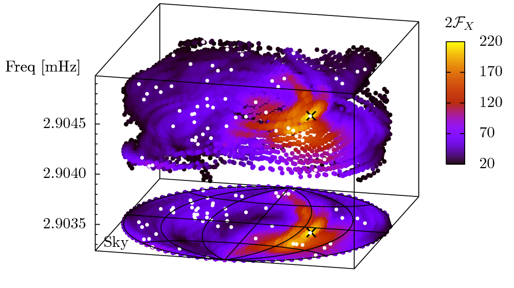
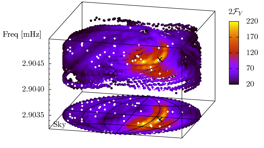
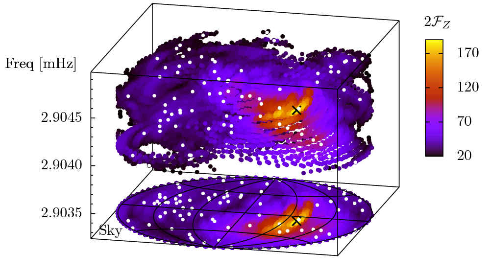
Both single- and multi-detector $\mathcal{F}$-statistic searches are complicated by the presence of secondary maxima in Doppler parameter space, i.e., points where $\mathcal{F}$ reaches a substantial local maximum, separated from the primary maximum at Doppler parameters of the true signal. This is illustrated in figure 2 for a search with only one injected signal. If only one signal is present, the global maximum of $2\mathcal{F}$ can be identified as the parameters of the true signal. Our original MLDC1 search identified the loudest signal within a narrow frequency band as the true signal, but could not distinguish between secondary maxima due to that signal and weaker true signals nearby in frequency and at different points in the sky.

In constructing our MLDC2 pipelinePrix and Whelan (2007a), we observed empirically that the same source tended to generate different patterns in secondary maxima across the sky in the TDI variables $X$, $Y$, and $Z$. We thus identified “true” signal candidates by requiring them to have consistent Doppler parameters in single-detector searches performed using the $X$, $Y$, and $Z$ observables. (The noise correlation among those three observables is irrelevant because this stage involves coincidences among the results of three single-detector searches rather than a coherent multi-detector search.) Note that a coherent multi-detector search involving $X$, $Y$ and $Z$ does not have this discriminating power, as it also yields a likelihood surface with primary and secondary maxima, similar to figure 2. The details of the coincidence criterion are discussed below, but it is based on requiring a low Doppler mismatch Prix (2007)

$$m=g_{ij}\delta\theta^{i}\delta\theta^{j}\sim 1-\frac{E\left[2\mathcal{F}(\theta+\delta\theta)\right]}{E\left[2\mathcal{F}(\theta)\right]}$$ (14)

between candidates in different single-detector searches. No condition was placed on the consistency of the recovered amplitude parameters, in part because the LW searches in particular are known to produce unreliable Doppler parameters. Once signals had been identified in coincidence between pairs of single-detector searches, those candidates were followed up with finer-gridded single-detector searches, and candidates surviving in coincidence were then targeted with a coherent multi-detector search using the noise-independent TDI combinations $X$ and $Y-Z$ as the two “detectors”.

The detailed pipeline was thus as follows:

• Wide parameter-space single-detector searches using each of the TDI variables $X$, $Y$, and $Z$. Up to $N=100,000$ Doppler parameter points with $2\mathcal{F}>2\mathcal{F}_{\text{th}}=20$ values are kept. Note that only one year of data is used in these initial single-detector stages. This was empirically found to cut down on false alarms.

• Identification of local maxima in each “detector”. A signal is a local maximum if there is no signal with higher $2\mathcal{F}$ value at a Doppler mismatch (14) of $m<m_{\text{LM}}=2$.

• Identification of coarse coincidences among the searches, using the coincidence condition $m<m_{\text{COINC1}}=0.8$. For our search of MLDC2 data, a set of candidates in the three detectors was considered to be in coincidence if each pair of candidates was within the prescribed mismatch.

• Followup of initial candidates with finer-gridded single-detector searches and tighter coincidence. The search “zooms in” by iteratively increasing the resolution of the Doppler parameter grid for each detector. At the end of this process, coincidence among the detectors is checked again with the tighter condition $m<m_{\text{COINC2}}=0.2$.

• Final multi-detector followup of surviving candidates. Now a multi-detector search is performed with the TDI combinations $X$ and $Y-Z$, which have independent noise contributions. As in stage four, the search “zooms in” on the true Doppler parameters iteratively. The ultimate resolution of the search is set by this multi-detector search, which uses the full two years of data.

III.2 Parameter Errorbars

We estimated the errors expected from Gaussian fluctuations of the noise using the Fisher information matrices on the amplitude and Doppler parameter subspaces. For the amplitude parameters, the expected discrepancy $\Delta\mathcal{A}=\mathcal{A}_{{\mathrm{c}}}-\mathcal{A}_{{\mathrm{s}}}$ between the parameters $\mathcal{A}_{{\mathrm{c}}}$ returned by the search and the true signal parameters $\mathcal{A}_{{\mathrm{s}}}$ is described by the expectation value

$$E\left[\Delta\mathcal{A}^{\mu}\Delta\mathcal{A}^{\nu}\right]=\mathcal{M}^{\mu\nu}(\theta_{\mathrm{s}})\,,$$ (15)

so we can quote an errorbar on a particular $\mathcal{A}^{\mu}$ of

$$\sigma_{\mathcal{A}^{\mu}}=\sqrt{\mathcal{M}^{\mu\mu}}\,,$$ (16)

with no implied sum over $\mu$ (we made no attempt to translate this back into errorbars on the physical parameters $h_{0}$, $\cos\iota$, $\psi$ and $\phi_{0}$).

Note, however, that this definition assumes that either the Doppler parameters $\theta_{\mathrm{s}}$ are perfectly matched by the candidate (i.e., $\theta_{\mathrm{c}}=\theta_{\mathrm{s}}$) or there are no correlations between amplitude- and Doppler-coordinates in the full parameter-space Fisher matrix. In practice none of these two conditions are satisfied in the present search. Therefore we expect deviations from these predicted error-distributions even in the case of perfectly Gaussian noise.

For the Doppler parameters, the expected discrepancy $\Delta\theta^{i}=\theta^{i}_{\mathrm{c}}-\theta^{i}_{\mathrm{s}}$, between the Doppler parameters $\theta^{i}_{\mathrm{c}}$ of the primary $2\mathcal{F}$ maximum and those $\theta^{i}_{\mathrm{c}}$ of the simulated signal is described by

$$E\left[\Delta\theta^{i}\Delta\theta^{j}\right]=\bar{\Gamma}^{ij}\,,$$ (17)

where $\bar{\Gamma}^{ij}$ is the inverse of the Fisher information matrix

$$\bar{\Gamma}_{ij}=g_{ij}\,\left\lvert\mathcal{A}_{{\mathrm{c}}}\right\rvert^{2}\,,$$ (18)

which can be defined in terms of the Doppler metric $g_{ij}$ associated with the mismatch (14). Similar to the error-estimates on amplitudes, this definition assumes either perfectly matched amplitude parameters (i.e., $\mathcal{A}_{{\mathrm{c}}}=\mathcal{A}_{{\mathrm{s}}}$) or a block-diagonal Fisher matrix over the full parameter space, with no correlations between amplitude- and Doppler-space. In practice none of these conditions is true and we therefore expect deviations from the predicted error estimates.

Rather than the full $\mathcal{F}$-statistic metric, we use the approximate orbital metric Prix (2007). This metric is approximated having constant elements in terms of the coordinates $\{\omega_{0},k_{x},k_{y}\}$ where

$$\omega_{0} =2\pi f\,,$$ (19a)

$$k_{x} =-2\pi f\frac{v_{\text{orb}}}{c}\cos\beta\cos\lambda\,,$$ (19b)

$$k_{y} =-2\pi f\frac{v_{\text{orb}}}{c}\cos\beta\sin\lambda\,.$$ (19c)

A limitation of the orbital metric is that it cannot distinguish between the points $\{f,\beta,\lambda\}$ and $\{f,-\beta,\lambda\}$ which are reflected through the ecliptic. (The search itself can distinguish between points with different signs of ecliptic latitude, thanks to the different amplitude modulation, but this is not captured in the orbital metric.) Assigning error bars to the frequency $f$ and ecliptic longitude $\lambda$ is straightforward, but converting an uncertainty in $\cos\beta$ into an uncertainty in ecliptic latitude $\beta$ is complicated by the orbital metric becoming singular at the ecliptic. As a workaround, we first calculate error bars

$$\sigma_{f}^{2} =\frac{\partial f}{\partial\theta^{i}}\frac{\partial f}{\partial\theta^{j}}\bar{\Gamma}^{ij}\,,$$ (20a)

$$\sigma_{\lambda}^{2} =\frac{\partial\lambda}{\partial\theta^{i}}\frac{\partial\lambda}{\partial\theta^{j}}\bar{\Gamma}^{ij}\,,$$ (20b)

$$\sigma_{\cos\beta}^{2} =\frac{\partial\cos\beta}{\partial\theta^{i}}\frac{\partial\cos\beta}{\partial\theta^{j}}\bar{\Gamma}^{ij}\,,$$ (20c)

and then estimate the error in $$\beta$$ as

$$\sigma_{\beta}:=\cos^{-1}(\cos\beta-\sigma_{\cos\beta})-\left\lvert\beta\right\rvert\,,$$ (20d)

so that

$$cos(\left\lvert\beta\right\rvert+\sigma_{\beta})=\cos\beta+\sigma_{\cos\beta}\,,$$ (20e)

i.e., we match the one-sigma equation in the direction away from the ecliptic, where the conversion between $$\beta \cos\beta \sigma_{\beta}>\left\lvert\beta\right\rvert \pm 1\sigma$$ and should be well behaved. It is of course possible that , in which case the interval we define straddles the ecliptic, but this agrees qualitatively with the observation that some signals near the ecliptic are recovered in the opposite hemisphere.

IV Evaluation

IV.1 Signal Identification

When run on the MLDC 2.1 dataset, our pipeline returns $\sim 2000$ signals found in coincidence. To evaluate its performance, we check how many of those sources were found at parameters consistent with those of one of the galactic binary signals injected into the data. The original datasets were generated with $\sim 30\,$million signals, but of those 59401 were considered “bright” enough to detect by the MLDC Task Force and their parameters were placed into a separate key file. It is against that key that we compare our results.

In part due to the known inaccuracies in amplitude parameters associated with the long-wavelength and partial rigid adiabatic responses, we checked for consistency using only the Doppler parameters (frequency and sky position). A signal was considered to be “found” if the Doppler parameters of the candidate and the key had a mismatch

$$m_{{\mathrm{c}}{\mathrm{s}}}=g_{ij}\Delta\theta^{i}\Delta\theta^{j}$$ (21)

of 1 or less. (In the case of multiple injected and/or candidate signals satisfying the mismatch condition, the brightest were “paired off” first.) If no injected signal matched a candidate, that candidate was considered to be a “false alarm”.

IV.2 Parameter Errors

These expectation values (15) and (17) allow us to define, as in Whelan et al. (2008),

$$\epsilon_{\theta}=\sqrt{\frac{\bar{\Gamma}_{ij}}{3}\Delta\theta^{i}\Delta\theta^{j}}\,,$$ (22)

and

$$\epsilon_{\mathcal{A}}=\sqrt{\frac{\mathcal{M}_{\mu\nu}}{4}\Delta\mathcal{A}^{\mu}\Delta\mathcal{A}^{\nu}}=\frac{\left\lvert\Delta\mathcal{A}\right\rvert}{2}\,,$$ (23)

so that

$$E\left[\epsilon_{\theta}^{2}\right]=1=E\left[\epsilon_{\mathcal{A}}^{2}\right]\,,$$ (24)

in the ideal case of statistical errors due to Gaussian noise, and no correlations between amplitude- and Doppler-parameters.

V Results without signal subtraction

V.1 Signal Recovery

The signal recovery of our pipeline using the various response models is summarized in table 2. Note that signal recovery is not significantly affected by the scalar response function $R(f)$, so the pRA search performs almost identically to the LW one. (See section II.2 and table 1 for the definitions of the different models of the LISA response.) However, the use of the full response tensor ${\mathchoice{\mathord{\hbox to0.0pt{\hbox to8.79988pt{\hss$\displaystyle d$\hss}\hss}\raise 7.98605pt\hbox to8.79988pt{\hss\hbox{$\scriptstyle\leftrightarrow$}\hss}}}{\mathord{\hbox to0.0pt{\hbox to8.79988pt{\hss$\textstyle d$\hss}\hss}\raise 7.98605pt\hbox to8.79988pt{\hss\hbox{$\scriptstyle\leftrightarrow$}\hss}}}{\mathord{\hbox to0.0pt{\hbox to6.99988pt{\hss$\scriptstyle d$\hss}\hss}\raise 5.59023pt\hbox to6.99988pt{\hss\hbox{$\scriptscriptstyle\leftrightarrow$}\hss}}}{\mathord{\hbox to0.0pt{\hbox to6.99988pt{\hss$\scriptscriptstyle d$\hss}\hss}\raise 3.99301pt\hbox to6.99988pt{\hss\hbox{$\scriptscriptstyle\leftrightarrow$}\hss}}}}\mathord{}(f,\widehat{k})$ in the full RA search leads to an increase in the number of found signals from 1704 to 1989, with much of the improvement coming from higher-frequency signals, and a reduction in the number of false alarms. Note that while the designated “bright signals” key contained 59401 sources, many of those were still not bright by the standards of our search, having low values of $\left\lvert\mathcal{A}_{{\mathrm{s}}}\right\rvert^{2}$. Since the faintest signal found by our search had $2\mathcal{F}=\left\lvert\mathcal{A}_{{\mathrm{c}}}\right\rvert^{2}=69.4$, we focus attention on sources with $\left\lvert\mathcal{A}_{{\mathrm{s}}}\right\rvert^{2}\geq 40$, of which there are 6586 in the key file.

Freqs	Signals	Found			False
	($\left\lvert\mathcal{A}\right\rvert^{2}>40$)	RA	pRA	LW	RA	pRA	LW
0–5 mHz	4446	1025	984	982	2	1	1
5–10 mHz	1967	822	652	652	3	5	5
10–15 mHz	163	133	68	68	0	1	1
15–20 mHz	7	7	2	2	0	0	0
20–27 mHz	3	2	0	0	0	2	2
Total	6586	1989	1706	1704	5	9	9

Table 2: Comparison of galactic WDB signal recovery with long-wavelength (LW), partial rigid adiabatic (pRA) and full rigid adiabatic (RA) response. The pRA and LW response functions differ only in the scalar piece $R(f)$, and produce similarly efficient searches. The RA response, including the full response tensor ${\mathchoice{\mathord{\hbox to0.0pt{\hbox to8.79988pt{\hss$\displaystyle d$\hss}\hss}\raise 7.98605pt\hbox to8.79988pt{\hss\hbox{$\scriptstyle\leftrightarrow$}\hss}}}{\mathord{\hbox to0.0pt{\hbox to8.79988pt{\hss$\textstyle d$\hss}\hss}\raise 7.98605pt\hbox to8.79988pt{\hss\hbox{$\scriptstyle\leftrightarrow$}\hss}}}{\mathord{\hbox to0.0pt{\hbox to6.99988pt{\hss$\scriptstyle d$\hss}\hss}\raise 5.59023pt\hbox to6.99988pt{\hss\hbox{$\scriptscriptstyle\leftrightarrow$}\hss}}}{\mathord{\hbox to0.0pt{\hbox to6.99988pt{\hss$\scriptscriptstyle d$\hss}\hss}\raise 3.99301pt\hbox to6.99988pt{\hss\hbox{$\scriptscriptstyle\leftrightarrow$}\hss}}}}\mathord{}(f,\widehat{k})$, leads to more found signals and fewer false alarms, especially at higher frequencies.

V.2 Doppler parameter accuracy

As described in section IV.2, we can compare the Doppler parameters $\theta_{\mathrm{c}}$ of each candidate with those $\theta_{\mathrm{s}}$ of the corresponding signal in the key. The errors, as a function of candidate frequency, are shown in figure 3. We show the errors for the searches using the full (RA) and partial (pRA) rigid adiabatic responses. The Doppler parameters returned using the long-wavelength (LW) limit are almost identical to the pRA results, so we omit those. We plot the combined measure $\epsilon_{\theta}$ defined in (22) (which has $E\left[\epsilon_{\theta}^{2}\right]=1$ in the case of Gaussian statistical errors), the error $\Delta f$ in the measured frequency and the angle $\phi_{\text{sky}}$ between the recovered and actual sky positions.

Figure 3: Doppler parameter errors as a function of frequency. The left panel shows the error measure $\epsilon_{\theta}$ defined in (22) which is normalized to have expected unit RMS value in the case of perfectly matched amplitude parameters and statistical errors caused by Gaussian noise. The right panels show the errors in frequency and sky position. We show the errors for searches using the partial rigid adiabatic (pRA) and full rigid adiabatic (RA) responses. The Doppler errors using the naïve long-wavelength limit are nearly identical to the pRA results and are therefore omitted.

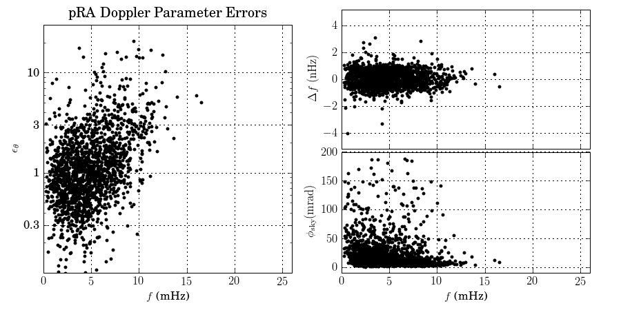
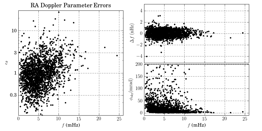
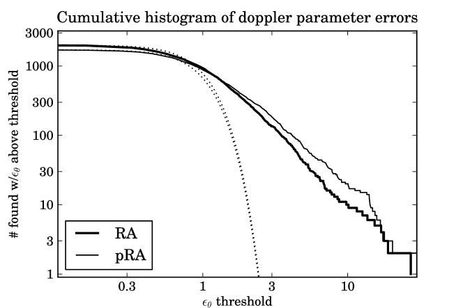
The pRA Doppler errors are seen to be a bit larger than the RA Doppler errors. We can quantify this by making a cumulative histogram of the Doppler error measure $\epsilon_{\theta}$ defined in (22). For statistical errors arising from Gaussian noise and neglecting amplitude-Doppler correlations, $3\epsilon_{\theta}^{2}$ should follow a central $\chi^{2}$ distribution with three degrees of freedom, i.e.,

$$P(\epsilon_{\theta}>\epsilon_{\theta}^{*})=\operatorname{erfc}\left(\epsilon_{\theta}^{*}\sqrt{\frac{3}{2}}\right)+\sqrt{\frac{6}{\pi}}\,\epsilon_{\theta}^{*}\,e^{-3{\epsilon_{\theta}^{*}}^{2}/2}\,.$$ (25)

The cumulative histograms of $\epsilon_{\theta}$ for the RA and pRA search, together with these theoretical expectations, are plotted in figure 4.

Figure 4: Cumulative histograms for Doppler parameter errors $\epsilon_{\theta}$ (see figure 3 for definitions). The dotted lines show the appropriately scaled theoretical CDF (25) in the case of perfectly matched amplitude parameters and statistical errors caused by Gaussian noise, where $3\epsilon_{\theta}^{2}$ follows a central $\chi^{2}$ distribution with three degrees of freedom.

V.3 Amplitude parameter accuracy

As described in section IV.2, we compare the vector of Amplitude parameters $\mathcal{A}_{{\mathrm{c}}}$ of each candidate with those $\mathcal{A}_{{\mathrm{s}}}$ of the corresponding signal in the key. The natural geometrical structure for studying those vectors is the metric $\mathcal{M}_{\mu\nu}$. (For concreteness we use $\mathcal{M}_{\mu\nu}(\theta_{\mathrm{s}})$, i.e. evaluated at the Doppler parameters of the signal in the key). We can use the quantity $\epsilon_{\mathcal{A}}$ defined in (23) (which has $E\left[\epsilon_{\mathcal{A}}^{2}\right]=1$ in the case of Gaussian statistical errors and perfectly matched Doppler parameters) as a measure of the overall discrepancy. We can also separate out the discrepancy in the length of the amplitude vectors from the angle between them in the four-dimensional amplitude parameter space, using quantities defined in Whelan et al. (2008):

$${\delta_{\mathcal{A}}}\equiv\frac{\left\lvert\mathcal{A}_{{\mathrm{c}}}\right\rvert^{2}-\left\lvert\mathcal{A}_{{\mathrm{s}}}\right\rvert^{2}-4}{2\,\left\lvert\mathcal{A}_{{\mathrm{s}}}\right\rvert^{2}}$$ (26)

is a measure of the amplitude discrepancy designed to have $E\left[{\delta_{\mathcal{A}}}\right]=0$, while

$${\phi_{\mathcal{A}}}\equiv\cos^{-1}\left(\frac{\mathcal{A}_{{\mathrm{c}}}^{\mu}\mathcal{M}_{\mu\nu}\mathcal{A}_{{\mathrm{s}}}^{\nu}}{\left\lvert\mathcal{A}_{{\mathrm{c}}}\right\rvert\left\lvert\mathcal{A}_{{\mathrm{s}}}\right\rvert}\right)$$ (27)

measures the angle between the amplitude parameter vectors, and can be thought of as a phase discrepancy. Both ${\delta_{\mathcal{A}}}$ and ${\phi_{\mathcal{A}}}$ have expected standard deviation $\left\lvert\mathcal{A}_{{\mathrm{s}}}\right\rvert^{-1}$ in the case of Gaussian statistical errors.

In figure 5, figure 6, and figure 7 we plot $\epsilon_{\mathcal{A}}$, ${\delta_{\mathcal{A}}}$ and ${\phi_{\mathcal{A}}}$ for the signals recovered in the LWL, pRA, and RA searches, respectively.

Figure 5: Amplitude parameter errors using the long-wavelength limit (LWL) approximation, as a function of frequency. The left panel shows the error measure $\epsilon_{\mathcal{A}}$ defined in (23) which is normalized to have expected unit RMS value in the case of statistical errors caused by Gaussian noise. The right panels show the errors in the magnitude and direction of the amplitude parameter vector, as measured by the amplitude difference ${\delta_{\mathcal{A}}}$ defined in (26) and the angle ${\phi_{\mathcal{A}}}$ between the true and recovered amplitude parameter vectors, defined in (27) Note the frequency-dependent systematic phase error ${\phi_{\mathcal{A}}}$ and loss in SNR (${\delta_{\mathcal{A}}}<0$), discussed in section V.3.

Figure 6: Amplitude parameter errors using the partial rigid adiabatic (pRA) approximation, as a function of frequency. The quantities shown are as in figure 5. Note the frequency-dependent systematic loss in SNR (${\delta_{\mathcal{A}}}<0$), discussed in section V.3.

Figure 7: Amplitude parameter errors using the full rigid adiabatic (RA) approximation, as a function of frequency. The quantities shown are as in figure 5. Note that the frequency-dependent systematic phase error seen in figure 5 and loss in SNR seen in figure 5 and figure 5 are absent, as discussed in section V.3.

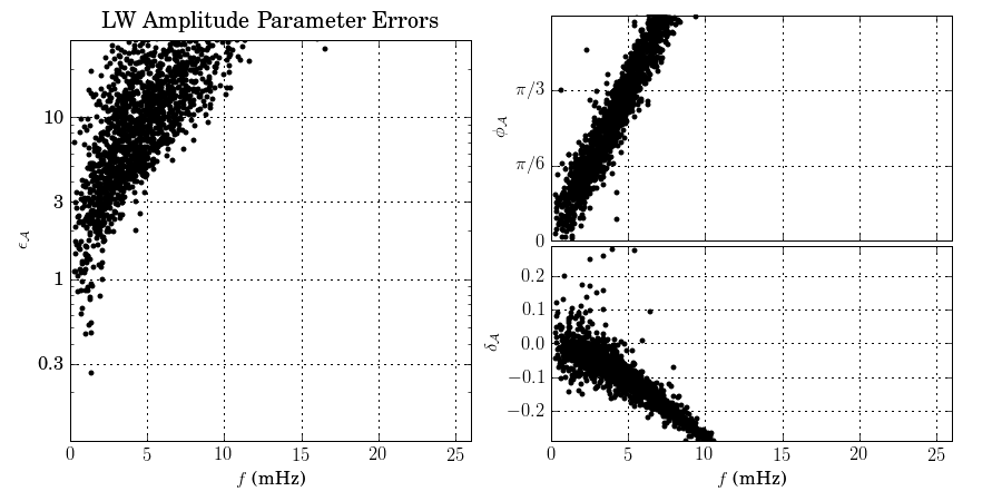
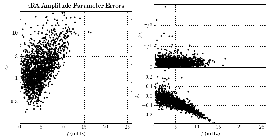
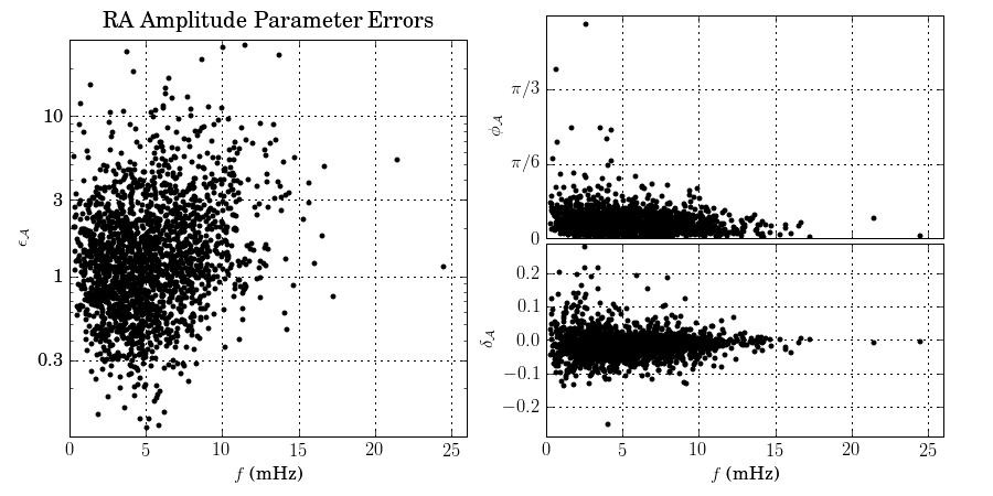
The LWL results have substantial systematic errors in both ${\delta_{\mathcal{A}}}$ and ${\phi_{\mathcal{A}}}$. The error in ${\phi_{\mathcal{A}}}$, which increases linearly with frequency, turns out to be mostly due to a systematic error in the initial phase $\phi_{0}$ corresponding to a time shift of $2T$. This problem can be traced to the absence of the factor of $e^{i4\pi fT}$ from (10) in the scalar response function $R_{\text{LWL}}(f)$ used in the LW search, and is fixed in the partial rigid adiabatic (pRA) approximation. There is also a systematic trend towards negative ${\delta_{\mathcal{A}}}$, which, recalling that $2\mathcal{F}=\left\lvert\mathcal{A}_{{\mathrm{c}}}\right\rvert^{2}$, corresponds to a signal being recovered with lower SNR than expected from the true amplitude parameters. Part of this effect is removed by the inclusion of $\operatorname{sinc}\left({2\pi fT}\right)$ in the denominator of (10), but the pRA results still show show a frequency-dependent SNR deficiency. Both effects are absent in the full RA search.

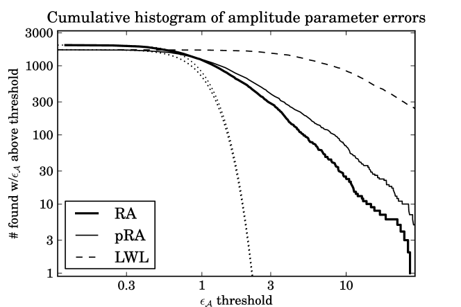
We can quantify the systematic errors, especially those still present in the RA search, by making a cumulative histogram of $\epsilon_{\mathcal{A}}$. For statistical errors arising from Gaussian noise (and neglecting amplitude-Doppler correlations), $4\epsilon_{\theta}^{2}$ should follow a central $\chi^{2}$ distribution with four degrees of freedom, i.e.,

$$P(\epsilon_{\mathcal{A}}>\epsilon_{\mathcal{A}}^{*})=e^{-2{\epsilon_{\mathcal{A}}^{*}}^{2}}\left(1+2{\epsilon_{\mathcal{A}}^{*}}^{2}\right)\,.$$ (28)

The cumulative histograms of $\epsilon_{\mathcal{A}}$ for the RA, pRA, and LWL searches, together with these theoretical expectations, are plotted in figure 8.

Figure 8: Cumulative histograms for Amplitude parameter errors $\epsilon_{\mathcal{A}}$ (see figure 7 for definitions). The dotted lines show the appropriately scaled theoretical CDF (28) in the case of statistical errors caused by Gaussian noise (and neglecting amplitude-Doppler correlations), where $4\epsilon_{\mathcal{A}}^{2}$ follows a central $\chi^{2}$ distribution with four degrees of freedom. The systematic errors illustrated by the non-Gaussian tails are greatly reduced by using the rigid adiabatic (RA) response.

V.4 Errors relative to estimated errorbars

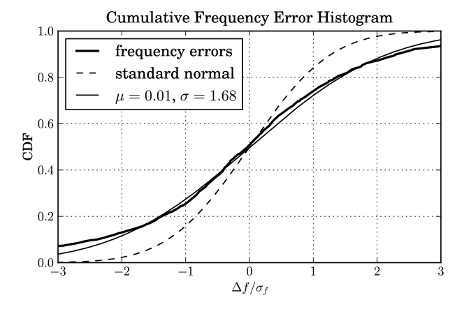
Another quantitative comparison of the size of the parameter errors to theoretical expectations is the ratio of the actual parameter errors $\Delta\mathcal{A}^{\mu}$ or $\Delta\theta^{i}$ to the errorbars $\sigma_{\mathcal{A}^{\mu}}$ or $\sigma_{\theta^{i}}$ defined in section III.2. We plot these for the full rigid adiabatic search. In figure 9 we histogram the relative frequency errors $\Delta{f}/\sigma_{f}$ for the 1989 recovered signals. For comparison, we also plot the cumulative histogram for a standard normal distribution, and for one with a mean $0.01$ and standard deviation of $1.68$, the values measured from the actual $\Delta{f}/\sigma_{f}$ distribution. In figure 10 we make similar histograms of the errors in the galactic latitude $\beta$ and longitude $\lambda$. We see that while the errors in sky location are comparable in scale to the computed errorbars, the frequency errors are slightly larger than expected, with a standard deviation of 1.68 (rather than unity) on $\Delta{f}/\sigma_{f}$. (This error is of comparable size in the RA, pRA, and LW searches.)

Figure 9: Cumulative histogram of frequency errors as a fraction of the errorbars estimated according to (20a), for the full RA search. We plot the histogram of the actual values, along with those for two Gaussian distributions: one with unit variance and zero mean (standard normal) and one with a mean of $0.01$ and standard deviation of $1.68$, equal to those in the actual distribution of $\Delta{f}/\sigma_{f}$ values.

Figure 10: Cumulative histograms for errors in the recovered galactic latitude $\beta$ and longitude $\lambda$ as a fraction of the errorbars estimated according to (20d) and (20b), for the full RA search, along with Gaussian distributions for comparison as in figure 9.

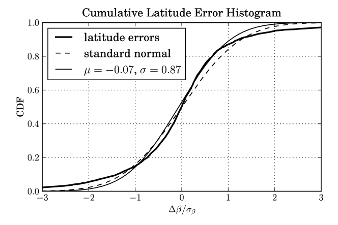
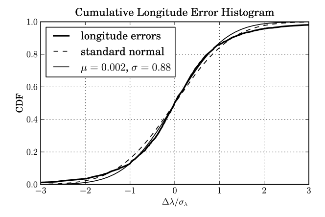
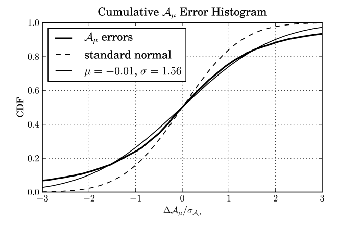
For the amplitude parameters, we collect together $\{\Delta\mathcal{A}^{\mu}/\sigma_{\mathcal{A}^{\mu}}|\mu=1,2,3,4\}$ for each of the 1989 recovered signals, and histogram those 7956 values. We see a slight systematic excess in these errors, with a standard deviation of 1.56 on the distribution of $\Delta\mathcal{A}^{\mu}/\sigma_{\mathcal{A}^{\mu}}$ values. This is smaller than the corresponding value of 2.21 from the pRA search and much smaller than the 15.22 found in the LW search. Replacing the long-wavelength approximation with the full rigid adiabatic response gives us amplitude parameters we can trust.

Figure 11: Cumulative histogram of the errors in all amplitude parameters $\mathcal{A}^{\mu}$ a fraction of the errorbars estimated according to (16), for the full RA search, along with Gaussian distributions for comparison as in figure 10.

VI Results with signal subtraction

A known limitation of our search pipeline is that it identifies individual signals, treating all of the other signals as background noise. One proposed approach is to generate signals corresponding to the candidates returned by a search of the data, subtract those from the data, and re-run the search on the resulting residuals. (This approach is a pedestrian alternative to the multiple-signal templates used in Crowder and Cornish (2007b, a).) This approach is only likely to work in a search which returns reliable signal parameters, and so we did not attempt it with our original long-wavelength-approximation pipeline. However, since the pipeline using the rigid adiabatic response generates very few false alarms, and reasonable Doppler and amplitude parameter accuracy, we can use it for a simple, illustrative signal subtraction program. The algorithm we use is as follows:

1. Run the original dataset through the standard pipeline described in section III to obtain a set of candidate signals.

2. Invert the amplitude parameter vectors ($\mathcal{A}^{\mu}\longrightarrow-\mathcal{A}^{\mu}$) of the candidate signals, and use those parameters to generate a composite signal to cancel out the signals found so far. For this step we used the lisatools MLDC Task Force (b) routines used to generate the original challenge data, in particular the FastGalaxy code Cornish and Littenberg (2007) and synthetic LISA Vallisneri .

3. Add this cancellation data set to the original MLDC data and generate a new set of SFTs with the found signals subtracted out.

4. Run the signal-subtracted dataset through the standard pipeline to obtain a set of “new” candidate signals.

5. Compare the new signals with the signals already found to distinguish duplicates (corresponding to unmatched residual portions of signals) from truly new signals. This is done using the same matching criterion used to compare found signals with a key, described in section IV.1. In this step, duplicates are analogous to “matched” signals and truly new signals are analogous to “false alarms”.

6. Combine the old and new signal lists to obtain a master list of signals found so far. Duplicates are only listed once, using the Doppler parameters with which they were found in the original search, and combined amplitude parameter vectors $\mathcal{A}^{\mu}_{\text{old}}+\mathcal{A}^{\mu}_{\text{new}}$.

7. Repeat the process from step 2, using the new master list of signals found so far to subtract from the original dataset.

The results of the iterative procedure are shown in table 3. We performed seven rounds of iterative subtraction and re-analysis (stopping the process at that point because the last round only added two new signals). This procedure increased the number of “true” signals found from 1989 to 3419, but also increased the false alarm rate, with the number of false alarms going from 5 to 29. This increase in the false alarm rate is not surprising, since we are looking for the weaker signals that remain after the brightest ones have been removed.

Rounds of Subtraction	0	1	2	3	4	5	6	7
Found Signals	1989	2962	3250	3346	3392	3405	3417	3419
False Alarms	5	23	24	27	28	28	29	29

Table 3: Results of iterative signal subtraction, described in section VI.

VII Comparison to Entries in the Second Mock LISA Data Challenge

An earlier version of this pipeline, using the long-wavelength approximation, was used to generate our entry in the second Mock LISA Data Challenge Prix and Whelan (2007a). Several other MLDC2 entries analyzed the same data set, as described in Babak et al. (2008a). The parameters returned by those “blind” searches are recorded at MLDC Task Force (c), and can be compared to the present pipeline using the criteria described in section IV. A script to do this is in the MLDCevaluation/Galaxy_Evaluation/AEI directory of lisatools MLDC Task Force (b), and we have run this on the entries, along with suitably converted versions of the searches reported in section V and section VI. For brevity we only report the numbers of false alarms and false dismissals, which are summarized in table 4.

Search	MTJPL	PWAEI	IMPAN	UTB	LW	RA	RAsubt
Found Signals	18084	1766	264	281	1704	1989	3419
False Alarms	1240	11	140	3581	9	5	29

Table 4: Comparison of different entries in the Second Mock LISA Data Challenge, and results of the current pipeline. The MLDC2 entries, which are described in Babak et al. (2008a) and available from MLDC Task Force (c), are: “MTJPL”, a submission by Crowder et al Crowder and Cornish (2007b, a) using the Metropolis-Hastings Monte Carlo with a multi-signal template; “PWAEI”, a submission by two of the present authors (Prix and Whelan) using a version of the present pipeline with the long-wavelength response Prix and Whelan (2007a); “IMPAN”, a submission by Królak and Błaut using an $\mathcal{F}$-statistic method Krolak et al. (2004) which was refined for subsequent MLDC rounds Blaut et al. (2009a, b); and “UTB”, a submission by Nayak et al using a tomographic method to map the overall distribution of galactic binaries Nayak et al. (2007). Included for comparison are “LW”, the present search with the long-wavelength response; “RA”, the present search with the rigid adiabatic response; and “RAsubt”, the search described in section VI with seven rounds of signal subtraction.

Our original MLDC entry returned the second highest number of true signals. While the UTB entry included more candidate signals than ours, very few of them were associated with actual sources according to the method of section IV.1. Incidentally, the same qualitative information carried in the right-hand panel Figure 1 of Babak et al. (2008a) is reflected in table 4, which considers the match between Doppler parameters of candidate signals and sources in the key: the PWAEI candidates have the lowest false alarm percentage, most of the 18084 MTJPL signals are real, and the UTB signals, in addition to having no amplitude parameter information and not determining the sign of the ecliptic latitude, have no discernible one-to-one correlation with the true sources.

The results of our original MLDC entry (“PWAEI”) are similar to the LW results reported in section V, but not identical because the original search used the LISA simulator data, and the present search uses data from synthetic LISA. The addition of the rigid adiabatic response makes a drastic improvement in amplitude parameter recovery as detailed in section V.3, but also increases the number of recovered signals, as does the experimental iterative signal subtraction technique detailed in section VI. The various incarnations of our pipeline recovered between 1704 and 3419 of the 59401 “bright” signals present in the data set (which contained a further 30 million background signals assumed to be undetectable); note, however, that due to our current pipeline first-stage threshold of $2\mathcal{F}>20$ (see Sec. III.1) we only expect to be able to find at most 6586 or so signals with $\left\lvert\mathcal{A}_{{\mathrm{s}}}\right\rvert^{2}\geq 40$. The MTJPL search by Crowder et al was able to recover 18084 true signals. This is still less than 59401, so the a priori assessment of “bright” signals should be taken with a grain of salt. However, the MTJPL pipeline also only missed 49 of those 6586 signals with $\left\lvert\mathcal{A}_{{\mathrm{s}}}\right\rvert^{2}\geq 40$, which indicates a higher intrinsic efficiency.

One advantage of our pipeline is speed. The full search can run in a matter of hours using a few hundred nodes of a computing cluster. The iterative signal subtraction was run over the course of a week, but much of that was taken up in subtracting signals and re-starting the pipeline by hand. The speed will also be affected by the choice of first-stage threshold in our pipeline (currently $2\mathcal{F}>20$). We could increase the number of signals found by lowering this threshold, but the next-stage follow-up steps and signal-subtraction would then take more time. More work would be required to understand how much efficiency could be gained at what computing cost by lowering this threshold, and how it would affect the quality and reliablity of signal extraction.

VIII Conclusions

We have applied an $\mathcal{F}$-statistic template bank search to mock LISA data containing a full galaxy of simulated white-dwarf binary systems. A multi-stage pipeline requiring Doppler parameter coincidence between searches using different TDI variables is effective in distinguishing true signals from false alarms and allows 1989 signals to be recovered with only 5 false alarms.

The use of the rigid adiabatic model for LISA response, including a response tensor depending on signal frequency and sky direction, eliminates the systematic amplitude parameter errors associated with searches using a long-wavelength approximation, and also allows more signals to be identified than with the simpler long-wavelength response tensor.

The relatively accurate recovery of both amplitude and Doppler parameters allows an experimental implementation of an iterative signal subtraction pipeline; after seven rounds of signal subtraction and re-analysis, the number of found signals was increased to 3419, with a total of 29 false alarms.