Multiple-relaxation-time lattice Boltzmann model for compressible fluids

Abstract

We present an energy-conserving multiple-relaxation-time finite difference lattice Boltzmann model for compressible flows. This model is based on a 16-discrete-velocity model. The collision step is first calculated in the moment space and then mapped back to the velocity space. The moment space and corresponding transformation matrix are constructed according to the group representation theory. Equilibria of the nonconserved moments are chosen according to the need of recovering compressible Navier-Stokes equations through the Chapman-Enskog expansion. Numerical experiments showed that compressible flows with strong shocks can be well simulated by the present model. The used benchmark tests include (i) shock tubes, such as the Sod, Lax, Colella explosion wave, collision of two strong shocks and a new shock tube with high mach number, (ii) regular and Mach shock reflections, (iii) shock wave reaction on cylindrical bubble problems, and (iv)Couette flow. The new model works for both low and high speeds compressible flows. It contains more physical information and has better numerical stability and accuracy than its single-relaxation-time version.

I Introduction

The Lattice Boltzmann (LB) method is an innovative numerical scheme originated from Lattice Gas Automata (LGA)1 and aim to simulate various hydrodynamics2 . The LB method was introduced to overcome some serious deficiencies of LGA, such as intrinsic noise, limited values of transport coefficients, non-Galilean invariance, and implementation difficulty in three dimensions. In the past two decades, most of the LB models are based on the famous Bhatnagar-Gross-Krook (BGK) approximation5 where a Single Relaxation Time (SRT) is used. Due to its validity and simplicity, the SRT LB method has been widely used to simulate various fluid flow problems, such as the multiphase flowShanChen ; Swift ; XGL1 ; XGL2 ; XGL6 ; XSB ; SS2007 ; Xu2009 , magnetohydrodynamicsPRL1991 ; 7 ; 8 ; PRA1991 ; PRE2002 ; PRE2004 ; CiCP2008 , flows through porous media9 ; 10 ; 10a and thermal fluid dynamics11 ; 11a ; 12 , etc.

However, the extreme simplicity of the SRT leads also to some constraints for the SRT LB model. For example, the simulation will be unstable when the relaxation time $\tau$ is close to 0.5, the model works only for low Mach number flows. One possible remedy is to use the Multiple Relaxation Time (MRT) methodHSB ; 13 . In real fluid the equilibrating rates of mass, momentum, energy, etc. are generally different. This difference can be manifested by the non-unique adjustable parameters in the MRT LB model. In contrast to the SRT model, the MRT version has much more adjustable parameters and degrees of freedom. The relaxation rates of various processes owing to particle collisions may be adjusted independently. The main strategy of the MRT LB scheme is that the collision step is first calculated in the moment space and then mapped back to the velocity space. The advection step is still computed in the velocity space. In many cases, it has been shown by Luo, et al17 ; 19 that the MRT LB model has better numerical stability.

Recently, the MRT LB method has attracted considerable interest and much progress has been achieved. For example, MRT models for viscoelastic fluids15 ; 16 ; 16a , multiphase flows20 ; 200 , flow with free surfaces18 , etc. were developed; optimal boundary condition for MRT LB was composed14 . To simulate system with temperature field, Luo, et al.19 suggested a hybrid thermal MRT LB model. These models work only for nearly incompressible fluids with very low Mach number.

LB community has long been attempting to construct models for compressible fluidsAlexander1 ; li1 ; sun1 ; yan1 . Alexander and Chen et al.Alexander1 constructed a model where the sound speed is adjustable so that the Mach number can be enhanced. Li, et al.li1 gave a model by reforming the velocity space. Sun, et al.sun1 formulated adaptive LB models where the particle velocities are determined by the mean velocity and internal energy. Yan, et al. yan1 proposed three-speed-three-energy-level models. Besides the standard LB mentioned above, some researchers have also tried to develop Finite Difference (FD) LB for compressible fluids20a ; 21a ; 2a , but in the real simulations the accessible Mach number is still not large. The model introduced by Kataoka and Tsutahara21a uses only sixteen discrete velocities and hence has a high computational efficiency.

The low-Mach number constraint is generally related to a numerical stability problem. The latter has been partly addressed by a number of techniques, such as the entropic method16+ ; 17+ , the fix-up scheme16+ ; 18+ , Flux-limitersSofonea1 and dissipation43 ; Brownlee1 techniques. In existing SRT models, it seems that the most effective solution to overcome the low Mach number constraint is to introduce artificial viscosity. But with the artificial viscosity, some fundamental kinetics are not very clear. In many cases, the MRT formulation has been shown to offer improved numerical stability, and provide additional physics. In this paper we present an energy-conserving multiple relaxation time finite difference lattice Boltzmann model for compressible flows with high Mach number. This model is based on the one proposed by Kataoka and Tsutahara21a . The moment space and transformation matrix are constructed according to the group representation theory. Equilibria of the nonconserved moments in the moment space are chosen when recovering compressible Navier-Stokes (NS) equations through the Chapman-Enskog (CE) expansion.

This paper is organized as follows. In Sect. II a brief review to the MRT LB model is presented. In Sect. III the new model is constructed. The von Neumann stability analysis is given in Sect. IV. Section V shows the numerical tests and some simulation results. Section VI provides a summary and concludes the paper.

II Brief review of the MRT LB model

The evolution of the distribution function $f_{i}$ for the particle velocity $v_{i}$ is governed by the following equation:

$$\frac{\partial f_{i}}{\partial t}+v_{i\alpha}\frac{\partial f_{i}}{\partial x_{\alpha}}=-\mathbf{S}_{ik}\left[f_{k}-f_{k}^{eq}\right]\text{,}$$ (1)

where $f_{i}$ ($f_{i}^{eq}$) is the particle (equilibrium) distribution function, $v_{i}$ represents a group of particle velocities, subscript $i$ indicates the particle’s direction, $i=1,\ldots,N$, $N$ is the number of discrete velocities, the subscript $\alpha$ indicates $x$ or $y$ component, $\mathbf{S}$ is the collision matrix. The equation reduces to the usual lattice BGK equation if all the relaxation parameters are set to be a single relaxation time $\tau$, namely $\mathbf{S}=\frac{1}{\tau}\mathbf{I}$, where $\mathbf{I}$ is the identity matrix.

The discrete (equilibrium) distribution function $f_{i}$ ($f_{i}^{eq}$) in Eq. (1) can be listed with the following matrixes:

$$\mathbf{f}=\left(f_{1},f_{2},\cdots,f_{N}\right)^{T}\text{,}$$ (2a)

$$\mathbf{f}^{eq}=\left(f_{1}^{eq},f_{2}^{eq},\cdots,f_{N}^{eq}\right)^{T}\text{,}$$ (2b)

where $$T$$ is the transpose operator.

Given a set of discrete velocities $v_{i}$, and corresponding distribution functions $f_{i}$, we can get a velocity space $S^{V}$, spanned by discrete velocities $v_{i}$, and a moment space $S^{M}$, spanned by moments of particle distribution function $f_{i}$, where $i=1,\cdots,N$. Similarly, we also express the moments of distribution function with the column matrix: $\hat{\mathbf{f}}=\left(\hat{f}_{1},\hat{f}_{2},\cdots,\hat{f}_{N}\right)^{T}$, where $\hat{f}_{i}=m_{ij}f_{j}$, $m_{ij}$ is an element of the matrix $\mathbf{M}$ and is a polynomial of discrete velocities. Obviously, the moments are simply linear combination of distribution functions$\ f_{i}$, and the mapping between moment space and velocity space is defined by the linear transformation $\mathbf{M}$, i.e., $\hat{\mathbf{f}}=\mathbf{Mf}$, $\mathbf{f=M}^{-1}\hat{\mathbf{f}}$, where $\mathbf{M}=\left(m_{1},m_{2},\cdots,m_{N}\right)^{T},m_{i}=(m_{i1},m_{i2},\cdots,m_{iN})$.

The LB simulation consists of two steps: the collision step and the advection one. In the MRT LB method, the advection step is computed in the velocity space. The collision step is first calculated in the moment space and then mapped to the velocity space. So, the MRT LB equation can be described as:

$$\frac{\partial f_{i}}{\partial t}+v_{i\alpha}\frac{\partial f_{i}}{\partial x_{\alpha}}=-\mathbf{M}_{il}^{-1}\hat{\mathbf{S}}_{lk}(\hat{f}_{k}-\hat{f}_{k}^{eq})\text{,}$$ (3)

where $\hat{\mathbf{S}}=\mathbf{MSM}^{-1}=diag(s_{1},s_{2},\cdots,s_{N})$ is the diagonal relaxation matrix. $\hat{f}_{i}^{eq}$ is the equilibrium value of the moment $\hat{f}_{i}$. The moments can be divided into two groups. The first group consists of the moments locally conserved in the collision process, i.e. $\hat{f}_{i}=\hat{f}_{i}^{eq}$. The second group consists of the moments not conserved, i.e. $\hat{f}_{i}\neq\hat{f}_{i}^{eq}$. The equilibrium $\hat{f}_{i}^{eq}$ is a function of conserved moments.

III Energy-conserving MRT LB model

We use the two-dimensional discrete velocity model by Kataoka and Tsutahara21a (see Fig. 1). It can be expressed as:

$$\left(v_{i1},v_{i2}\right)=\left\{\begin{array}[]{cc}\mathbf{cyc}:\left(\pm 1,0\right)\text{,}&\text{for }1\leq i\leq 4\text{,}\\ \mathbf{cyc}:\left(\pm 6,0\right)\text{,}&\text{for }5\leq i\leq 8\text{,}\\ \sqrt{2}\left(\pm 1,\pm 1\right)\text{,}&\text{for }9\leq i\leq 12\text{,}\\ \frac{3}{\sqrt{2}}\left(\pm 1,\pm 1\right)\text{,}&\text{for }13\leq i\leq 16\text{,}\end{array}\right.$$ (4)

where cyc indicates the cyclic permutation.

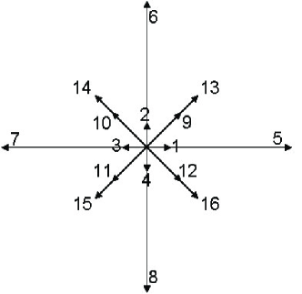
Figure 1: Distribution of $\mathbf{v}_{i\alpha}$ for the discrete velocity model.

III.1 Construction of transformation matrix $\mathbf{M}$

The transformation matrix $\mathbf{M}$ is constructed according to the irreducible representations of SO(2) group:

$$1\text{,}$$

$$\cos\theta\text{,}\sin\theta\text{,}$$

$$\sin^{2}\theta+\cos^{2}\theta\text{,}\cos 2\theta\text{,}\sin 2\theta\text{,}$$

$$\cos\theta(\sin^{2}\theta+\cos^{2}\theta)\text{,}\sin\theta(\sin^{2}\theta+\cos^{2}\theta)\text{,}\cos 3\theta\text{,}\sin 3\theta\text{,}$$

$$(\sin^{2}\theta+\cos^{2}\theta)^{2}\text{,}\cos 2\theta(\sin^{2}\theta+\cos^{2}\theta)\text{,}\sin 2\theta(\sin^{2}\theta+\cos^{2}\theta)\text{,}\cos 4\theta\text{,}\sin 4\theta\text{,}$$

$$\cdots$$

Let $v_{ix}$ and $v_{iy}$ play the roles of $\cos\theta$ and $\sin\theta$, respectively. Then we define

$$m_{1i}=1\text{,}$$ (5a)

$$m_{2i}=v_{ix}\text{,}$$ (5b)

$$m_{3i}=v_{iy}\text{,}$$ (5c)

$$m_{4i}=(v_{ix}^{2}+v_{iy}^{2})/2\text{,}$$ (5d)

$$m_{5i}=v_{ix}^{2}-v_{iy}^{2}\text{,}$$ (5e)

$$m_{6i}=v_{ix}v_{iy}\text{,}$$ (5f)

$$m_{7i}=v_{ix}(v_{ix}^{2}+v_{iy}^{2})/2\text{,}$$ (5g)

$$m_{8i}=v_{iy}(v_{ix}^{2}+v_{iy}^{2})/2\text{,}$$ (5h)

$$m_{9i}=v_{ix}(v_{ix}^{2}-3v_{iy}^{2})\text{,}$$ (5i)

$$m_{10i}=v_{iy}(3v_{ix}^{2}-v_{iy}^{2})\text{,}$$ (5j)

$$m_{11i}=(v_{ix}^{2}+v_{iy}^{2})^{2}/4\text{,}$$ (5k)

$$m_{12i}=v_{ix}^{4}-6v_{ix}^{2}v_{iy}^{2}+v_{iy}^{4}\text{,}$$ (5l)

$$m_{13i}=(v_{ix}^{2}+v_{iy}^{2})(v_{ix}^{2}-v_{iy}^{2})\text{,}$$ (5m)

$$m_{14i}=(v_{ix}^{2}+v_{iy}^{2})v_{ix}v_{iy}\text{,}$$ (5n)

$$m_{15i}=v_{ix}(v_{ix}^{2}-3v_{iy}^{2})(v_{ix}^{2}+v_{iy}^{2})\text{,}$$ (5o)

$$m_{16i}=v_{iy}(3v_{ix}^{2}-v_{iy}^{2})(v_{ix}^{2}+v_{iy}^{2})\text{.}$$ (5p)

where $$i=1,\cdots,16$$.

For two-dimensional compressible models, we have four conserved moments, density $\rho$, momentums $j_{x}$, $j_{y}$, and energy $e$. They are denoted by $\hat{f}_{1}$, $\hat{f}_{2}$, $\hat{f}_{3}$ and $\hat{f}_{4}$, respectively. Specifically, $\hat{f}_{1}=\rho=\sum f_{i}m_{1i}$, $\hat{f}_{2}=j_{x}=\sum f_{i}m_{2i}$, $\hat{f}_{3}=j_{y}=\sum f_{i}m_{3i}$, $\hat{f}_{4}=e=\sum f_{i}m_{4i}$. To be consistent with the idiomatic expression of energy, in the definitions of $m_{4i}$, $m_{7i}$ and $m_{8i}$, a coefficient $1/2$ is used. Similarly, a coefficient $1/4$ is used in the definition of $m_{11i}$. Thus, the transformation matrix $\mathbf{M}$ can be expressed as follows:

$$\mathbf{M}=(m_{1},m_{2},\cdots,m_{16})^{T}\text{,}$$

where

$$m_{1}=(1,1,1,1,1,1,1,1,1,1,1,1,1,1,1,1)\text{,}$$

$$m_{2}=(1,0,-1,0,6,0,-6,0,\sqrt{2},-\sqrt{2},-\sqrt{2},\sqrt{2},\frac{3}{\sqrt{2}},-\frac{3}{\sqrt{2}},-\frac{3}{\sqrt{2}},\frac{3}{\sqrt{2}})\text{,}$$

$$m_{3}=(0,1,0,-1,0,6,0,-6,\sqrt{2},\sqrt{2},-\sqrt{2},-\sqrt{2},\frac{3}{\sqrt{2}},\frac{3}{\sqrt{2}},-\frac{3}{\sqrt{2}},-\frac{3}{\sqrt{2}})\text{,}$$

$$m_{4}=(\frac{1}{2},\frac{1}{2},\frac{1}{2},\frac{1}{2},18,18,18,18,2,2,2,2,\frac{9}{2},\frac{9}{2},\frac{9}{2},\frac{9}{2})\text{,}$$

$$m_{5}=(1,-1,1,-1,36,-36,36,-36,0,0,0,0,0,0,0,0)\text{,}$$

$$m_{6}=(0,0,0,0,0,0,0,0,2,-2,2,-2,\frac{9}{2},-\frac{9}{2},\frac{9}{2},-\frac{9}{2})\text{,}$$

$$m_{7}=(\frac{1}{2},0,-\frac{1}{2},0,108,0,-108,0,2\sqrt{2},-2\sqrt{2},-2\sqrt{2},2\sqrt{2},\frac{27}{2\sqrt{2}},-\frac{27}{2\sqrt{2}},-\frac{27}{2\sqrt{2}},\frac{27}{2\sqrt{2}})\text{,}$$

$$m_{8}=(0,\frac{1}{2},0,-\frac{1}{2},0,108,0,-108,2\sqrt{2},2\sqrt{2},-2\sqrt{2},-2\sqrt{2},\frac{27}{2\sqrt{2}},\frac{27}{2\sqrt{2}},-\frac{27}{2\sqrt{2}},-\frac{27}{2\sqrt{2}})\text{,}$$

$$m_{9}=(1,0,-1,0,216,0,-216,0,-4\sqrt{2},4\sqrt{2},4\sqrt{2},-4\sqrt{2},-\frac{27}{\sqrt{2}},\frac{27}{\sqrt{2}},\frac{27}{\sqrt{2}},-\frac{27}{\sqrt{2}})\text{,}$$

$$m_{10}=(0,-1,0,1,0,-216,0,216,4\sqrt{2},4\sqrt{2},-4\sqrt{2},-4\sqrt{2},\frac{27}{\sqrt{2}},\frac{27}{\sqrt{2}},-\frac{27}{\sqrt{2}},-\frac{27}{\sqrt{2}})\text{,}$$

$$m_{11}=(\frac{1}{4},\frac{1}{4},\frac{1}{4},\frac{1}{4},324,324,324,324,4,4,4,4,\frac{81}{4},\frac{81}{4},\frac{81}{4},\frac{81}{4})\text{,}$$

$$m_{12}=(1,1,1,1,1296,1296,1296,1296,-16,-16,-16,-16,-81,-81,-81,-81)\text{,}$$

$$m_{13}=(1,-1,1,-1,1296,-1296,1296,-1296,0,0,0,0,0,0,0,0)\text{,}$$

$$m_{14}=(0,0,0,0,0,0,0,0,8,-8,8,-8,\frac{81}{2},-\frac{81}{2},\frac{81}{2},-\frac{81}{2})\text{,}$$

$$m_{15}=(1,0,-1,0,7776,0,-7776,0,-16\sqrt{2},16\sqrt{2},16\sqrt{2},-16\sqrt{2},-\frac{243}{\sqrt{2}},\frac{243}{\sqrt{2}},\frac{243}{\sqrt{2}},-\frac{243}{\sqrt{2}})\text{,}$$

$$m_{16}=(0,-1,0,1,0,-7776,0,7776,16\sqrt{2},16\sqrt{2},-16\sqrt{2},-16\sqrt{2},\frac{243}{\sqrt{2}},\frac{243}{\sqrt{2}},-\frac{243}{\sqrt{2}},-\frac{243}{\sqrt{2}})\text{.}$$

III.2 Determination of $\hat{f}_{i}^{eq}$

We perform the Chapman-Enskog expansion20 ; 22 ; 23 on the two sides of Eq.(1). We define

$$f_{i}=f_{i}^{(0)}+f_{i}^{(1)}+f_{i}^{(2)}\text{,}$$ (6a)

$$\frac{\partial}{\partial t}=\frac{\partial}{\partial t_{1}}+\frac{\partial}{\partial t_{2}}\text{,}$$ (6b)

$$\frac{\partial}{\partial x}=\frac{\partial}{\partial x_{1}}\text{,}$$ (6c)

where $$f_{i}^{(0)} f_{i}^{(1)} \frac{\partial}{\partial t_{1}} \frac{\partial}{\partial x_{1}} f_{i}^{(2)} \frac{\partial}{\partial t_{2}} \epsilon \epsilon$$ is the zeroth order, , and  are the first order,  and are the second order terms of the Knudsen number . Equating the coefficients of the zeroth, the first, and the second order terms in gives

$$f_{i}^{(0)}=f_{i}^{eq}\text{,}$$ (7a)

$$(\frac{\partial}{\partial t_{1}}+v_{i\alpha}\frac{\partial}{\partial x_{1\alpha}})f_{i}^{(0)}=-\mathbf{S}_{il}f_{l}^{(1)}\text{,}$$ (7b)

$$\frac{\partial}{\partial t_{2}}f_{i}^{(0)}+(\frac{\partial}{\partial t_{1}}+v_{i\alpha}\frac{\partial}{\partial x_{1\alpha}})f_{i}^{(1)}=-\mathbf{S}_{il}f_{l}^{(2)}\text{.}$$ (7c)

They can be converted into moment space to obtain:

$$\hat{f}_{i}^{(0)}=\hat{f}_{i}^{eq}\text{,}$$ (8a)

$$(\frac{\partial}{\partial t_{1}}+\hat{\mathbf{E}}_{\alpha}\frac{\partial}{\partial x_{1\alpha}})\hat{f}_{i}^{(0)}=-\hat{\mathbf{S}}_{il}\hat{f}_{l}^{(1)}\text{,}$$ (8b)

$$\frac{\partial}{\partial t_{2}}\hat{f}_{i}^{(0)}+(\frac{\partial}{\partial t_{1}}+\hat{\mathbf{E}}_{\alpha}\frac{\partial}{\partial x_{1\alpha}})\hat{f}_{i}^{(1)}=-\hat{\mathbf{S}}_{il}\hat{f}_{l}^{(2)}\text{,}$$ (8c)

where $$\hat{\mathbf{E}}_{\alpha}=\mathbf{M}(v_{i\alpha}\mathbf{I})\mathbf{M}^{-1}$$.

The equilibria of the moments in the moment space can be defined as : $\hat{\mathbf{f}}^{eq}=(\rho,j_{x},j_{y},e,\hat{f}_{5}^{eq},\hat{f}_{6}^{eq},\cdots,\hat{f}_{16}^{eq})^{T}$. The first order deviations from equilibria are defined as : $\hat{\mathbf{f}}^{(1)}=(0,0,0,0,\hat{f}_{5}^{(1)},\hat{f}_{6}^{(1)},\cdots,\hat{f}_{16}^{(1)})^{T}$. In the same way, the second order deviations are $\hat{\mathbf{f}}^{(2)}=(0,0,0,0,\hat{f}_{5}^{(2)},\hat{f}_{6}^{(2)},\cdots,\hat{f}_{16}^{(2)})^{T}$. From Eq.(8b) we obtain

$$\frac{\partial\rho}{\partial t_{1}}+\frac{\partial j_{x}}{\partial x_{1}}+\frac{\partial j_{y}}{\partial y_{1}}=0\text{,}$$ (9a)

$$\frac{\partial j_{x}}{\partial t_{1}}+\frac{\partial}{\partial x_{1}}(e+\frac{1}{2}\hat{f}_{5}^{eq})+\frac{\partial}{\partial y_{1}}\hat{f}_{6}^{eq}=0\text{,}$$ (9b)

$$\frac{\partial j_{y}}{\partial t_{1}}+\frac{\partial}{\partial x_{1}}\hat{f}_{6}^{eq}+\frac{\partial}{\partial y_{1}}(e-\frac{1}{2}\hat{f}_{5}^{eq})=0\text{,}$$ (9c)

$$\frac{\partial e}{\partial t_{1}}+\frac{\partial}{\partial x_{1}}\hat{f}_{7}^{eq}+\frac{\partial}{\partial y_{1}}\hat{f}_{8}^{eq}=0\text{,}$$ (9d)

$$\frac{\partial}{\partial t_{1}}\hat{f}_{5}^{eq}+\frac{\partial}{\partial x_{1}}(\hat{f}_{7}^{eq}+\frac{1}{2}\hat{f}_{9}^{eq})+\frac{\partial}{\partial y_{1}}(-\hat{f}_{8}^{eq}+\frac{1}{2}\hat{f}_{10}^{eq})=-s_{5}\hat{f}_{5}^{(1)}\text{,}$$ (9e)

$$\frac{\partial}{\partial t_{1}}\hat{f}_{6}^{eq}+\frac{1}{4}\frac{\partial}{\partial x_{1}}(2\hat{f}_{8}^{eq}+\hat{f}_{10}^{eq})+\frac{1}{4}\frac{\partial}{\partial y_{1}}(2\hat{f}_{7}^{eq}-\hat{f}_{9}^{eq})=-s_{6}\hat{f}_{6}^{(1)}\text{,}$$ (9f)

$$\frac{\partial}{\partial t_{1}}\hat{f}_{7}^{eq}+\frac{\partial}{\partial x_{1}}(\hat{f}_{11}^{eq}+\frac{1}{4}\hat{f}_{13}^{eq})+\frac{1}{2}\frac{\partial}{\partial y_{1}}\hat{f}_{14}^{eq}=-s_{7}\hat{f}_{7}^{(1)}\text{,}$$ (9g)

$$\frac{\partial}{\partial t_{1}}\hat{f}_{8}^{eq}+\frac{1}{2}\frac{\partial}{\partial x_{1}}\hat{f}_{14}^{eq}+\frac{\partial}{\partial y_{1}}(\hat{f}_{11}^{eq}-\frac{1}{4}\hat{f}_{13}^{eq})=-s_{8}\hat{f}_{8}^{(1)}\text{,}$$ (9h)

$$\frac{\partial}{\partial t_{1}}\hat{f}_{9}^{eq}+\frac{1}{2}\frac{\partial}{\partial x_{1}}(\hat{f}_{12}^{eq}+\hat{f}_{13}^{eq})-\frac{\partial}{\partial y_{1}}\hat{f}_{14}^{eq}=-s_{9}\hat{f}_{9}^{(1)}\text{,}$$ (9i)

$$\frac{\partial}{\partial t_{1}}\hat{f}_{10}^{eq}+\frac{\partial}{\partial x_{1}}\hat{f}_{14}^{eq}+\frac{1}{2}\frac{\partial}{\partial y_{1}}(-\hat{f}_{12}^{eq}+\hat{f}_{13}^{eq})=-s_{10}\hat{f}_{10}^{(1)}\text{,}$$ (9j)

$$\frac{\partial}{\partial t_{1}}\hat{f}_{11}^{eq}+\frac{\partial}{\partial x_{1}}(-9j_{x}+\frac{25}{2}\hat{f}_{7}^{eq}+3\hat{f}_{9}^{eq})+\frac{\partial}{\partial y_{1}}(-9j_{y}+\frac{25}{2}\hat{f}_{8}^{eq}-3\hat{f}_{10}^{eq})=-s_{11}\hat{f}_{11}^{(1)}\text{,}$$ (9k)

$$\frac{\partial}{\partial t_{1}}\hat{f}_{12}^{eq}+\frac{\partial}{\partial x_{1}}\hat{f}_{15}^{eq}-\frac{\partial}{\partial y_{1}}\hat{f}_{16}^{eq}=-s_{12}\hat{f}_{12}^{(1)}\text{,}$$ (9l)

$$\frac{\partial}{\partial t_{1}}\hat{f}_{13}^{eq}+\frac{\partial}{\partial x_{1}}(-18j_{x}+\frac{1}{2}\hat{f}_{15}^{eq}+25\hat{f}_{7}^{eq}+6\hat{f}_{9}^{eq})+\frac{\partial}{\partial y_{1}}(18j_{y}+\frac{1}{2}\hat{f}_{16}^{eq}-25\hat{f}_{8}^{eq}+6\hat{f}_{10}^{eq})=-s_{13}\hat{f}_{13}^{(1)}\text{,}$$ (9m)

$$\frac{\partial}{\partial t_{1}}\hat{f}_{14}^{eq}+\frac{\partial}{\partial x_{1}}(-9j_{y}+\frac{1}{4}\hat{f}_{16}^{eq}+\frac{25}{2}\hat{f}_{8}^{eq}-3\hat{f}_{10}^{eq})-\frac{\partial}{\partial y_{1}}(9j_{x}+\frac{1}{4}\hat{f}_{15}^{eq}-\frac{25}{2}\hat{f}_{7}^{eq}-3\hat{f}_{9}^{eq})=-s_{14}\hat{f}_{14}^{(1)}\text{,}$$ (9n)

$$\frac{\partial}{\partial t_{1}}\hat{f}_{15}^{eq}+\frac{\partial}{\partial x_{1}}(75e-54\rho-18\hat{f}_{5}^{eq}+18\hat{f}_{11}^{eq}+\frac{25}{2}\hat{f}_{12}^{eq}+\frac{37}{2}\hat{f}_{13}^{eq})+\frac{\partial}{\partial y_{1}}(36\hat{f}_{6}^{eq}-13\hat{f}_{14}^{eq})=-s_{15}\hat{f}_{15}^{(1)}\text{,}$$ (9o)

$$\frac{\partial}{\partial t_{1}}\hat{f}_{16}^{eq}-\frac{\partial}{\partial x_{1}}(36\hat{f}_{6}^{eq}-13\hat{f}_{14}^{eq})-\frac{\partial}{\partial y_{1}}(75e-54\rho+18\hat{f}_{5}^{eq}+18\hat{f}_{11}^{eq}+\frac{25}{2}\hat{f}_{12}^{eq}-\frac{37}{2}\hat{f}_{13}^{eq})=-s_{16}\hat{f}_{16}^{(1)}\text{.}$$ (9p)

From Eq.(8c) we obtain

$$\frac{\partial\rho}{\partial t_{2}}=0\text{,}$$ (10a)

$$\frac{\partial j_{x}}{\partial t_{2}}+\frac{1}{2}\frac{\partial}{\partial x_{1}}\hat{f}_{5}^{(1)}+\frac{\partial}{\partial y_{1}}\hat{f}_{6}^{(1)}=0\text{,}$$ (10b)

$$\frac{\partial j_{y}}{\partial t_{2}}+\frac{\partial}{\partial x_{1}}\hat{f}_{6}^{(1)}-\frac{1}{2}\frac{\partial}{\partial y_{1}}\hat{f}_{5}^{(1)}=0\text{,}$$ (10c)

$$\frac{\partial e}{\partial t_{2}}+\frac{\partial}{\partial x_{1}}\hat{f}_{7}^{(1)}+\frac{\partial}{\partial y_{1}}\hat{f}_{8}^{(1)}=0\text{.}$$ (10d)

Adding Eq.(10) and the first four formulas of Eq.(9) leads to the following equations,

$$\frac{\partial\rho}{\partial t}+\frac{\partial j_{x}}{\partial x}+\frac{\partial j_{y}}{\partial y}=0\text{,}$$ (11a)

$$\frac{\partial j_{x}}{\partial t}+\frac{\partial}{\partial x}(e+\frac{1}{2}\hat{f}_{5}^{eq})+\frac{\partial}{\partial y}\hat{f}_{6}^{eq}=-\frac{1}{2}\frac{\partial}{\partial x}\hat{f}_{5}^{(1)}-\frac{\partial}{\partial y}\hat{f}_{6}^{(1)}\text{,}$$ (11b)

$$\frac{\partial j_{y}}{\partial t}+\frac{\partial}{\partial x}\hat{f}_{6}^{eq}+\frac{\partial}{\partial y}(e-\frac{1}{2}\hat{f}_{5}^{eq})=-\frac{\partial}{\partial x}\hat{f}_{6}^{(1)}+\frac{1}{2}\frac{\partial}{\partial y}\hat{f}_{5}^{(1)}\text{,}$$ (11c)

$$\frac{\partial e}{\partial t}+\frac{\partial}{\partial x}\hat{f}_{7}^{eq}+\frac{\partial}{\partial y}\hat{f}_{8}^{eq}=-\frac{\partial}{\partial x}\hat{f}_{7}^{(1)}-\frac{\partial}{\partial y}\hat{f}_{8}^{(1)}\text{.}$$ (11d)

To obatin the NS equations, we choose

$$\hat{f}_{5}^{eq}=(j_{x}^{2}-j_{y}^{2})/\rho\text{,}$$ (12a)

$$\hat{f}_{6}^{eq}=j_{x}j_{y}/\rho\text{,}$$ (12b)

$$\hat{f}_{7}^{eq}=(e+P)j_{x}/\rho\text{,}$$ (12c)

$$\hat{f}_{8}^{eq}=(e+P)j_{y}/\rho\text{,}$$ (12d)

$$\hat{f}_{9}^{eq}=(j_{x}^{2}-3j_{y}^{2})j_{x}/\rho^{2}\text{,}$$ (12e)

$$\hat{f}_{10}^{eq}=(3j_{x}^{2}-j_{y}^{2})j_{y}/\rho^{2}\text{,}$$ (12f)

$$\hat{f}_{11}^{eq}=2e^{2}/\rho-(j_{x}^{2}+j_{y}^{2})^{2}/4\rho^{3}\text{,}$$ (12g)

$$\hat{f}_{13}^{eq}=(6\rho e-2j_{x}^{2}-2j_{y}^{2})(j_{x}^{2}-j_{y}^{2})/\rho^{3}\text{,}$$ (12h)

$$\hat{f}_{14}^{eq}=(6\rho e-2j_{x}^{2}-2j_{y}^{2})j_{x}j_{y}/\rho^{3}\text{.}$$ (12i)

The definitions of $$\hat{f}_{12}^{eq} \hat{f}_{15}^{eq} \hat{f}_{16}^{eq} \hat{f}_{12}^{eq}=\hat{f}_{15}^{eq}=\hat{f}_{16}^{eq}=0$$, ,  have no effect on macroscopic equations, so we can choose . In this way the recovered NS equations are as follows:

$$\frac{\partial\rho}{\partial t}+\frac{\partial j_{x}}{\partial x}+\frac{\partial j_{y}}{\partial y}=0\text{,}$$ (13a)

$$\frac{\partial j_{x}}{\partial t}+\frac{\partial}{\partial x}\left(j_{x}^{2}/\rho\right)+\frac{\partial}{\partial y}\left(j_{x}j_{y}/\rho\right)=-\frac{\partial P}{\partial x}+\frac{\partial}{\partial x}[\mu_{s}(\frac{\partial u_{x}}{\partial x}-\frac{\partial u_{y}}{\partial y})]+\frac{\partial}{\partial y}[\mu_{v}(\frac{\partial u_{y}}{\partial x}+\frac{\partial u_{x}}{\partial y})]\text{,}$$ (13b)

$$\frac{\partial j_{y}}{\partial t}+\frac{\partial}{\partial x}\left(j_{x}j_{y}/\rho\right)+\frac{\partial}{\partial y}\left(j_{y}^{2}/\rho\right)=-\frac{\partial P}{\partial y}+\frac{\partial}{\partial x}[\mu_{v}(\frac{\partial u_{y}}{\partial x}+\frac{\partial u_{x}}{\partial y})]-\frac{\partial}{\partial y}[\mu_{s}(\frac{\partial u_{x}}{\partial x}-\frac{\partial u_{y}}{\partial y})]\text{,}$$ (13c)

$$\frac{\partial e}{\partial t}+\frac{\partial}{\partial x}[(e+P)j_{x}/\rho]+\frac{\partial}{\partial y}[(e+P)j_{y}/\rho]$$ (13d)

$$= \frac{\partial}{\partial x}[\lambda_{1}(2\frac{\partial T}{\partial x}+u_{y}\frac{\partial u_{y}}{\partial x}+u_{x}\frac{\partial u_{x}}{\partial x}-u_{x}\frac{\partial u_{y}}{\partial y}+u_{y}\frac{\partial u_{x}}{\partial y})]$$

$$+\frac{\partial}{\partial y}[\lambda_{2}(2\frac{\partial T}{\partial y}+u_{x}\frac{\partial u_{x}}{\partial y}-u_{y}\frac{\partial u_{x}}{\partial x}+u_{x}\frac{\partial u_{y}}{\partial x}+u_{y}\frac{\partial u_{y}}{\partial y})]\text{,}$$

where $$\mu_{s}= \rho RT/s_{5} \mu_{v}= \rho RT/s_{6} \lambda_{1}=\rho RT/s_{7} \lambda_{2}=\rho RT/s_{8} \mu_{s}= \mu_{v}=\mu \lambda_{1}=\lambda_{2}=\lambda$$ , , , . When  , , the above NS equations reduce to

$$\frac{\partial\rho}{\partial t}+\frac{\partial j_{\alpha}}{\partial x_{\alpha}}=0\text{,}$$ (14a)

$$\frac{\partial j_{\alpha}}{\partial t}+\frac{\partial\left(j_{\alpha}j_{\beta}/\rho\right)}{\partial x_{\beta}}=-\frac{\partial P}{\partial x_{\alpha}}+\frac{\partial}{\partial x_{\beta}}[\mu(\frac{\partial u_{\alpha}}{\partial x_{\beta}}+\frac{\partial u_{\beta}}{\partial x_{\alpha}}-\frac{\partial u_{\chi}}{\partial x_{\chi}}\delta_{\alpha\beta})]\text{,}$$ (14b)

$$\frac{\partial e}{\partial t}+\frac{\partial}{\partial x_{\alpha}}[(e+P)j_{\alpha}/\rho]=\frac{\partial}{\partial x_{\alpha}}[\lambda(2\frac{\partial T}{\partial x_{\alpha}}+u_{\beta}(\frac{\partial u_{\alpha}}{\partial x_{\beta}}+\frac{\partial u_{\beta}}{\partial x_{\alpha}}-\frac{\partial u_{\chi}}{\partial x_{\chi}}\delta_{\alpha\beta})]\text{.}$$ (14c)

IV Von Neumann Stability Analysis

In this section we perform the von Neumann stability analysis on the new MRT LB model. In the stability analysis, we write the solution of FD LB equation in the form of Fourier series. If all the eigenvalues of the coefficient matrix are less than 1, the algorithm is stable.

The distribution function $f_{i}(x_{\alpha},t)$ is split into two parts:

$$f_{i}(x_{\alpha},t)=\bar{f_{i}^{0}}+\Delta f_{i}(x_{\alpha},t)\text{,}$$ (15)

where $\bar{f_{i}^{0}}$ is the global equilibrium distribution function. It is a constant and does not vary with time or space, depends only on the average density, velocity and temperature. Similarly, the distribution function $\hat{f}_{i}(x_{\alpha},t)$ is split into two parts:

$$\hat{f}_{i}(x_{\alpha},t)=\hat{\bar{f_{i}^{0}}}+\Delta\hat{f}_{i}(x_{\alpha},t)\text{,}$$ (16)

where $\hat{\bar{f_{i}^{0}}}$ is a constant. Putting the Eq.(15) and Eq.(16) into Eq.(3) gives

$$\Delta f_{i}(x_{\alpha},t+\Delta t)=\Delta f_{i}(x_{\alpha},t)-\Delta tv_{i\alpha}\frac{\partial\Delta f_{i}}{\partial x_{\alpha}}-\Delta t\mathbf{M}_{il}^{-1}\hat{\mathbf{S}}_{lk}(\Delta\hat{f}_{k}-\Delta\hat{f}_{k}^{eq})\text{.}$$ (17)

The solution can be written as

$$\Delta f_{i}(x_{\alpha},t)=F_{i}^{t}\mathrm{exp}(\mathbf{i}k_{\alpha}x_{\alpha})\text{,}$$ (18)

where $F_{i}^{t}$ is an amplitude of sine wave at lattice point $x_{\alpha}$ and time $t$, $k_{\alpha}$ is the wave number. From the above two equations we can obtain $F_{i}^{t+\Delta t}=G_{ij}F_{j}^{t}.$ Coefficient matrix $G_{ij}$ describes the growth rate of amplitude $F_{i}^{t}$ in each time step $\Delta t$. If $\omega$ denotes the eigenvalue of coefficient matrix $G_{ij}$, the von Neumann stability condition is $\mathrm{max}|\omega|\leq 1$. Coefficient matrix $G_{ij}$ can be expressed as follows,

$$G_{ij} =\delta_{ij}-\frac{v_{i\alpha}\Delta t}{2\Delta x_{\alpha}}(e^{\mathbf{i}k_{\alpha}\Delta x_{\alpha}}-e^{-\mathbf{i}k_{\alpha}\Delta x_{\alpha}})\delta_{ij}+\frac{1}{2}(\frac{v_{i\alpha}\Delta t}{\Delta x_{\alpha}})^{2}(e^{\mathbf{i}k_{\alpha}\Delta x_{\alpha}}-2$$

$$+e^{-\mathbf{i}k_{\alpha}\Delta x_{\alpha}})\delta_{ij}-\Delta t\mathbf{M}_{il}^{-1}\hat{\mathbf{S}}_{lk}(\frac{\partial\hat{f}_{k}}{\partial f_{j}}-\frac{\partial\hat{f}_{k}^{eq}}{\partial f_{j}})\text{,}$$ (19)

where

$$\hat{f}_{k}=\mathbf{M}_{kp}f_{p}\text{,}$$

$$\frac{\partial\hat{f}_{k}^{eq}}{\partial f_{j}}=\frac{\partial\hat{f}_{k}^{eq}}{\partial\rho}\frac{\partial\rho}{\partial f_{j}}+\frac{\partial\hat{f}_{k}^{eq}}{\partial T}\frac{\partial T}{\partial f_{j}}+\frac{\partial\hat{f}_{k}^{eq}}{\partial u_{\alpha}}\frac{\partial u_{\alpha}}{\partial f_{j}}\text{.}$$ (20)

Coefficient matrix $G_{ij}$ contains a large number of matrix elements (as many as $16\times 16$), and every matrix element correlates with the macroscopic quantities and model parameters, so analytic analysis is very difficult. We conduct a quantitative analysis using Mathematica software.

In Fig.2 we show an example of stability comparison for the new MRT model and its SRT version. The abscissa is for $kdx$, and the vertical axis is for $|\omega|_{max}$ which is the largest eigenvalue of coefficient matrix $G_{ij}$. The macroscopic values in stability analysis are chosen as follows: $(\rho,u_{1},u_{2},T)$ = $(2.0,10.0,0.0,2.0)$, other common parameters are: $dx=dy=2\times 10^{-3}$, $dt=10^{-5}$. The relaxation time in SRT is $\tau=10^{-5}$, while the collision parameters in MRT are $s_{5}=6500$, $s_{7}=s_{8}=9\times 10^{4}$, $s_{9}=8\times 10^{4}$, $s_{13}=7\times 10^{4}$, $s_{14}=8\times 10^{3}$, $s_{15}=2.5\times 10^{4}$, the others are $10^{5}$. In this case, the MRT scheme is stable, while the SRT version is not. It is clear that, by choosing appropriate collision parameters, the stability of MRT can be much better than the SRT.

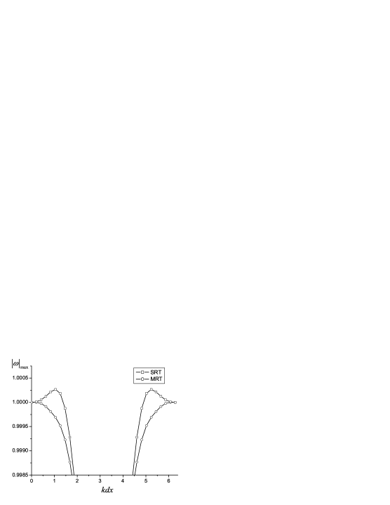
Figure 2: Stability comparison for the new MRT model and its SRT version.

V Numerical Simulations

In this section we study the following problems using the new MRT LB model: One-dimensional Riemann problems, shock reflections, shock wave reaction on cylindrical bubble, and Couette flow.

V.1 One-dimensional Riemann problems

Here, we study several typical one-dimensional Riemann problems, including the Sod, Lax shock tube, Colella explosion wave, collision of two strong shocks and a new shock tube with high Mach number. In the $x$ direction, $f_{i}=$ $f_{i}^{eq}$ is set on the boundary nodes before the disturbance reaches the two ends. In the $y$ direction, the periodic boundary condition is adopted. In the following part, subscripts “L” and “R” indicate the macroscopic variables at the left and right sides of discontinuity.

(a) Sod shock tube problem

The initial condition is

$$\left\{\begin{array}[]{cc}(\rho,u_{1},u_{2},T)|_{L}=(1.0,0.0,0.0,1.0)\text{,}&x\leq 0\text{.}\\ (\rho,u_{1},u_{2},T)|_{R}=(0.125,0.0,0.0,0.8)\text{,}&x>0\text{.}\end{array}\right.$$ (21)

Figure 3 shows a comparison of the MRT LB simulation results and exact solutions for the density, pressure, velocity and temperature of the Sod shock tube problem at time $t=0.18$. Here, in the collision matrix $s_{5}=s_{6}=5\times 10^{2}$, $s_{7}=s_{8}=10^{3}$, $s_{11}=2500$, and other collision parameters are$\ 10^{5}$. The red circles correspond to simulation results with the grid size $dx=dy=0.002$ and time step $dt=2\times 10^{-6}$ (case 1), the green triangles correspond to simulation results with $dx=dy=0.001$, $dt=10^{-6}$ (case 2), and solid lines represent the exact solutions. The relative errors of the density, pressure, velocity and temperature for case 1 are $0.234\%$, $0.182\%$, $3.32\%$ and $0.327\%$, respectively. The relative errors of the density, pressure, velocity and temperature for case 2 are $0.225\%$, $0.171\%$, $3.16\%$ and $0.322\%$, respectively. Here, the relative error is defined as $E=\sum_{I}\left|\varsigma_{{}_{I,J,num}}-\varsigma_{{}_{I,J,exa}}\right|/\sum_{I}\left|\varsigma_{{}_{I,J,exa}}\right|$, where $\varsigma_{{}_{I,J,num}}$ denotes the variables at the node of $(x_{I},y_{J})$ obtained from the numerical simulation, and $\varsigma_{{}_{I,J,exa}}$ is the exact solution at the same node. The simulation results successfully capture the main structure of the waves.

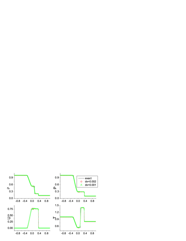
Figure 3: Comparison of the MRT LB simulation results and exact solutions for Sod shock tube at time $t=0.18$.

b) Lax shock tube problem

The initial condition of the problem is:

$$\left\{\begin{array}[]{cc}(\rho,u_{1},u_{2},T)|_{L}=(0.445,0.698,0.0,7.928)\text{,}&x\leq 0\text{.}\\ (\rho,u_{1},u_{2},T)|_{R}=(0.5,0.0,0.0,1.142)\text{,}&x>0\text{.}\end{array}\right.$$ (22)

Figure 4 shows the MRT LB numerical results and exact solutions for the Lax shock tube problem at time $t=0.2$. The red squares, green circles and blue triangles correspond to simulation results with different grid sizes and time steps: $dx=dy=0.004$, $dt=4\times 10^{-6}$ (case 1), $dx=dy=0.002$, $dt=2\times 10^{-6}$ (case 2), $dx=dy=0.001$, $dt=10^{-6}$ (case 3), respectively, and solid lines represent the exact solutions. The used parameters are $s_{7}=s_{8}=3\times 10^{3}$, $s_{13}=10^{2}$, other collision parameters are$\ 10^{5}$. The relative errors of the density, pressure, velocity and temperature for case 1 are $0.398\%$, $0.205\%$, $0.592\%$ and $0.310\%$, respectively. The relative errors for case 2 are $0.344\%$, $0.130\%$, $0.408\%$ and $0.287\%$, respectively. And the relative errors for case 3 are $0.334\%$, $0.117\%$, $0.372\%$ and $0.283\%$, respectively.

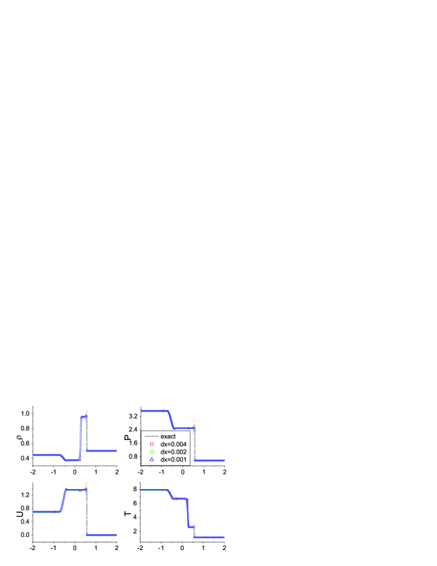
Figure 4: The MRT LB numerical and exact solutions for Lax shock tube at time $t=0.2$.

(c) Colella explosion wave

For the problem, the initial condition is

$$\left\{\begin{array}[]{cc}(\rho,u_{1},u_{2},T)|_{L}=(1.0,0.0,0.0,1000.0)\text{,}&x\leq 0\text{.}\\ (\rho,u_{1},u_{2},T)|_{R}=(1.0,0.0,0.0,0.01)\text{,}&x>0\text{.}\end{array}\right.$$ (23)

This is a strong temperature discontinuity problem that can be used to study the robustness and precision of numerical methods. Figure 5 gives density, pressure, velocity and temperature results at $t=0.1$. The red squares and green circles correspond to simulation results with different grid sizes and time steps: $dx=dy=0.002$, $dt=2\times 10^{-6}$ (case 1), and $dx=dy=0.001$, $dt=10^{-6}$ (case 2), respectively, and solid lines represent the exact solutions. Here, the parameters are $s_{7}=s_{8}=5\times 10^{4}$, $s_{11}=s_{13}=5\times 10^{5}$, other values of $s$ adopt $10^{5}$. The relative errors of the density, pressure, velocity and temperature for case 1 are $1.69\%$, $1.11\%$, $1.60\%$ and $0.779\%$, respectively. The relative errors for case 2 are $1.68\%$, $1.11\%$, $1.59\%$ and $0.777\%$, respectively. The oscillations at the interface are difficult to eliminate completely in our simulations.

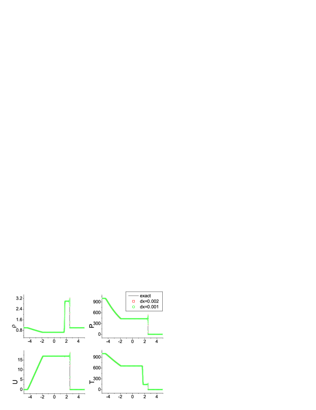
Figure 5: The MRT simulation results and exact solutions for the Colella explosion wave at time $t=0.1$.

(d) Collision of two strong shocks

The initial condition can be write as:

$$\left\{\begin{array}[]{cc}(\rho,u_{1},u_{2},T)|_{L}=(5.99924,19.5975,0.0,76.8254)\text{,}&x\leq 0\text{.}\\ (\rho,u_{1},u_{2},T)|_{R}=(5.99242,-6.19633,0.0,7.69222)\text{,}&x>0\text{.}\end{array}\right.$$ (24)

The MRT and SRT numerical results and exact solutions at time $t=0.1$ are shown in Fig.6, where the common parameters are $dx=dy=0.003$, $dt=10^{-5}$, the collision matrix in MRT is $s_{5}=s_{6}=5\times 10^{3}$, $s_{7}=s_{8}=3\times 10^{4}$, other values of $s$ are $10^{5}$, and the relaxation time in SRT is $\tau=10^{-5}$. The red squares and green circles correspond to the MRT and SRT simulation results, respectively, and solid lines represent the exact solutions. Compared with the simulation results of SRT, we can find that the oscillations at the discontinuity are weaker in MRT simulation.

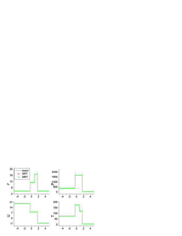
Figure 6: The MRT and SRT numerical results and exact solution for collision of two strong shocks at time $t=0.1$.

(e) High Mach number shock

In order to test the stability of the new model, we construct a new shock tube problem with the initial condition,

$$\left\{\begin{array}[]{cc}(\rho,u_{1},u_{2},T)|_{L}=(5.0,45.0,0.0,10.0)\text{,}&x\leq 0\text{.}\\ (\rho,u_{1},u_{2},T)|_{R}=(6.0,-20.0,0.0,5.0)\text{,}&x>0\text{.}\end{array}\right.$$ (25)

The Mach number of the left side is $10.1$, and the right is $6.3$. And this test is successfully passed by the MRT LB, but failed by the SRT. Figure 7 shows comparison of the MRT LB results and exact solutions at $t=0.018$, where the parameters are $dx=dy=0.003$, $dt=10^{-5}$, $s_{5}=s_{6}=1.5\times 10^{4}$, $s_{10}=5\times 10^{4}$, other values of $s$ are $10^{5}$. Circle symbols correspond to MRT simulation results, and solid lines represent the exact solutions.

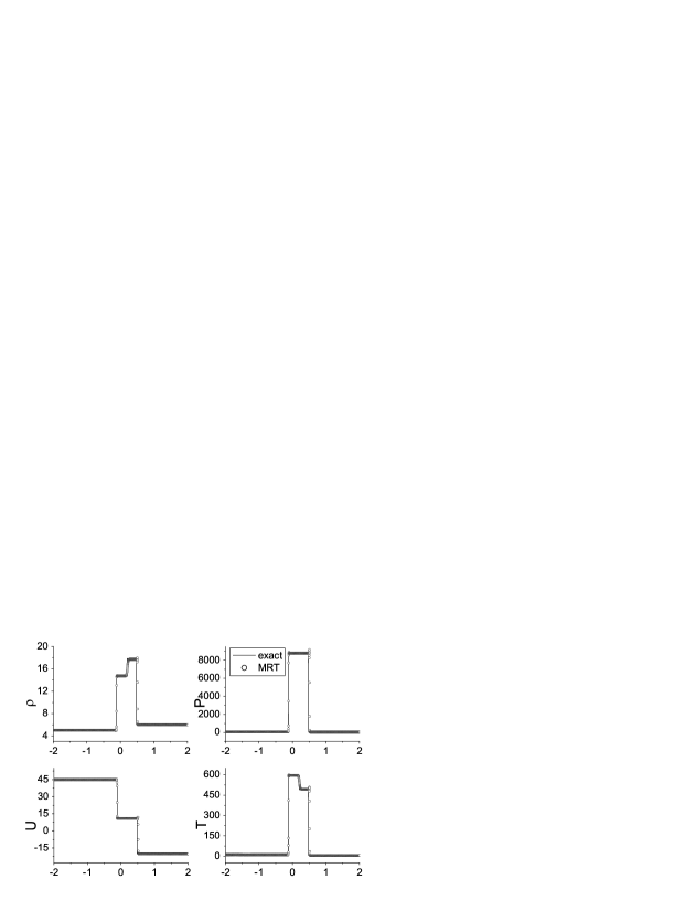
Figure 7: MRT LB results and exact solutions for the high Mach number shock tube problem at $t=0.018$.

V.2 Shock reflections

We adopt the macroscopic variable boundary conditions in Figs. 8-11. The values of the distribution functions on boundaries are assigned with the corresponding values of the equilibrium distribution functions. The determination methods of macroscopic quantities are explained combining with specific problems. Here we study two gas dynamic problems: regular and Mach shock reflections.

(a) Regular shock reflection

In the problem, we have performed a $30^{\circ}$ shock reflection, and the corresponding Mach number is $5$. The computational domain is a rectangle with length $0.6$ and height $0.2$, which is divided into $300\times 100.$ The reflecting wall lies at the bottom of the domain (reflecting boundary condition denotes the $y$ component of the fluid velocity on the boundary is reverse to that of interior point), and the linear extrapolation technique is applied to define the values of the macroscopic quantities on the right-hand boundary. The other two sides adopt the Dirichlet boundary conditions:

$$\left\{\begin{array}[]{l}(\rho\text{, }u_{1}\text{, }u_{2}\text{, }T)|_{0\text{, }y\text{, }t}=(1.0\text{, }5.0\text{, }0.0\text{, }0.5)\text{,}\\ (\rho\text{, }u_{1}\text{, }u_{2}\text{, }T)|_{x\text{, }0.2\text{, }t}=(2.27273\text{, }4.3\text{, -1.21244, 1.76})\text{.}\end{array}\right.$$ (26)

Initially, the entire interior zone is set the values of the left boundary. Parameters in the simulation are as follows: $dx=dy=0.002$, $dt=10^{-5}$, $s_{5}=10^{4}$, $s_{6}=2\times 10^{3}$, $s_{7}=s_{8}=10^{4}$, other collision parameters are $10^{5}$. Figure 8 shows the pressure contour at time $t=0.3$, and the density, temperature contours have similar results. From black to white, the grey level corresponds to the increase of the pressure. The result shows that the new MRT model has the ability to accurately capture the shock front.

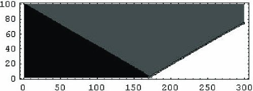
Figure 8: Pressure contour of regular shock reflection at time $t=0.3$.

(b) Mach reflection problem

This problem is on an unsteady shock reflection. A planar shock impacts an oblique surface which is at a $30^{\circ}$ angle to the propagation direction of the shock. The fluid in front of the shock has zero velocity, and the shock Mach number is $1.5$. The initial condition is as follows:

$$\left(\rho,u_{1},u_{2},T\right)\mid_{x\text{,}y\text{,}0}=\left\{\begin{array}[]{ll}(3.17647,0.555556\cos 30^{\circ},-0.555556\sin 30^{\circ},0.839506)\text{,}&\text{ if }y\geq h(x,0)\text{.}\\ (2.0,0.0,0.0,0.5)\text{,}&\text{ if }y<h(x,0)\text{.}\end{array}\right.$$ (27)

where $h(x,t)=\tan 60^{\circ}(x-150dx)-1.5t/\sin 30^{\circ}.$ The computational domain is divided into $600\times 300$. At the bottom boundary, reflecting boundary condition is used from the 150th grid, and the left side adopts the values of the initial post-shock flow; the left boundary is also assigned values of the initial post-shock flow, and at the right boundary the extrapolation technique is applied; at the top boundary, the macroscopic variables are assigned using the same method of the right boundary when $x>g(t)$, and are set the same values as the left boundary’s when $x\leq g(t)$, where $g(t)=150dx+\tan 30^{\circ}(0.9+1.5t/\sin 30^{\circ})$, $dx$ is the grid size in simulation. In Fig.9 we show the results of density, pressure, velocity in $x$ direction and temperature contours at $t=0.25$ in the part of $\left[50,450\right]\times\left[0,200\right]$. Parameters in the simulation are $dx=dy=0.003$, $dt=10^{-5}$, $s_{5}=10^{3}$, $s_{6}=5\times 10^{2}$, $s_{7}=s_{8}=10^{3}$, and other collision parameters are$\ 10^{5}$. The simulation results are accordant with those of other numerical methods41 ; 42 ; 43 ; CShuPRE .

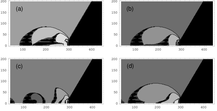
Figure 9: Mach reflection of shock wave. Figs. (a)-(d) shows the density, pressure, velocity in $x$ direction, and temperature at time $t=0.25$, respectively. From black to white, the grey level corresponds to the increase of values.

V.3 Shock wave reaction on cylindrical bubble problem

The problems are as follows: A planar shock wave with the Mach number $1.22$ impinges on a cylindrical bubble with different densities. In the first case the bubble has a lower density. In the second case the bubble’s density is higher.

Initial conditions for the first case are

$$\left(\rho,u_{1},u_{2},p\right)\mid_{x\text{,}y\text{,}0}=\left\{\begin{array}[]{cc}\left(1,0,0,1\right)\text{,}&\mathbf{pre-shock}\text{{,}}\\ \left(1.28,-0.3774,0,1.6512\right)\text{,}&\mathbf{post-shock}\text{{,}}\\ \left(0.1358,0,0,1\right)\text{,}&\mathbf{bubble}\text{{,}}\end{array}\right.$$ (28)

and for the second case are

$$\left(\rho,u_{1},u_{2},p\right)\mid_{x\text{,}y\text{,}0}=\left\{\begin{array}[]{cc}\left(1,0,0,1\right)\text{,}&\mathbf{pre-shock}\text{{,}}\\ \left(1.28,-0.3774,0,1.6512\right)\text{,}&\mathbf{post-shock}\text{{,}}\\ \left(3.1538,0,0,1\right)\text{,}&\mathbf{bubble}\text{{.}}\end{array}\right.$$ (29)

In the simulations, the right side adopts the values of the initial post-shock flow; the extrapolation technique is applied at the left boundary, and reflecting boundary conditions are imposed on the top and bottom. The common parameters are as follows: $dx=dy=0.003$, $dt=10^{-5}$. When simulate the low density cylindrical bubble, the collision parameters are $s_{5}=s_{6}=s_{7}=s_{8}=10^{4}$, and others are $10^{5}$; when simulate the high density bubble, the collision parameters are $s_{5}=10^{3}$, and $s=10^{5}$ for the others. In Fig. 10(a), from top to bottom, the three plots show the density contours at the times $t=0$, $0.5$, $0.65$, respectively. In Fig. 10(b), from top to bottom, the three plots show the density contours at the times $t=0$, $0.6$, $0.9$, respectively. These results are accordant with those from other methods24 and experiment24aa . The surface of bubbles is comparatively smooth, which indicates that the MRT modle has high accuracy and resolution.

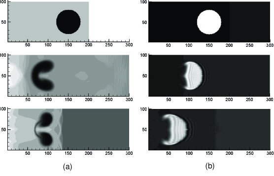
Figure 10: Snapshots of shock wave reaction on single bubble. The left column is for the process with initial condition (28), and the right column is for the process with initial condition (29). From black to white, the density value increases.

V.4 Couette flow

In order to demonstrate the accuracy of the model, numerical simulations of the incompressible Couette flow are carried out. Consider a viscous fluid flow between two infinite parallel flat plates, separated by a distance of $D$. The initial state of the fluid is $\rho=1$, $T=1$, $U=0$. At time $t=0$ the two plates start to move at velocities $U$, $-U$, respectively, ($U=0.1$). The periodic boundary condition is adopted in the x direction. The top and bottom boundaries are constant speed and constant temperature boundaries ($U=0.1,T=1$). The analytical solution of horizontal velocity along a vertical line is as follows:

$$u=2yU/D-\sum_{j}(-1)^{j+1}\frac{2U}{j\pi}\exp[-\frac{4j^{2}\pi^{2}\mu}{\rho D^{2}}t]\sin(\frac{2j\pi}{D}y)\text{,}$$

where $j$ is an integer, the two walls locate at $y=\pm D/2$.

We carried out a set of simulations: $dx=dy=0.004$, $dt=10^{-5}$, $NX\times NY=16\times 32$ (case 1), $dx=dy=0.002$, $dt=5\times 10^{-6}$, $NX\times NY=32\times 64$(case 2), $dx=dy=0.001$, $dt=2.5\times 10^{-6}$, $NX\times NY=64\times 128$ (case 3). All of the collision parameters are$\ 10^{5}$. Figure 11 shows a comparison of the MRT LB simulation results and exact solution for the horizontal velocity distribution at time $t=57.5$. The black squares, red triangles and green circles correspond to simulation results of case 1, case 2, and case 3, respectively, and solid line represents the exact solution. The relative errors of the horizontal velocity for the three cases are $7.02\%$, $3.86\%$ and $2.06\%$, respectively. So this model is of first order accuracy.

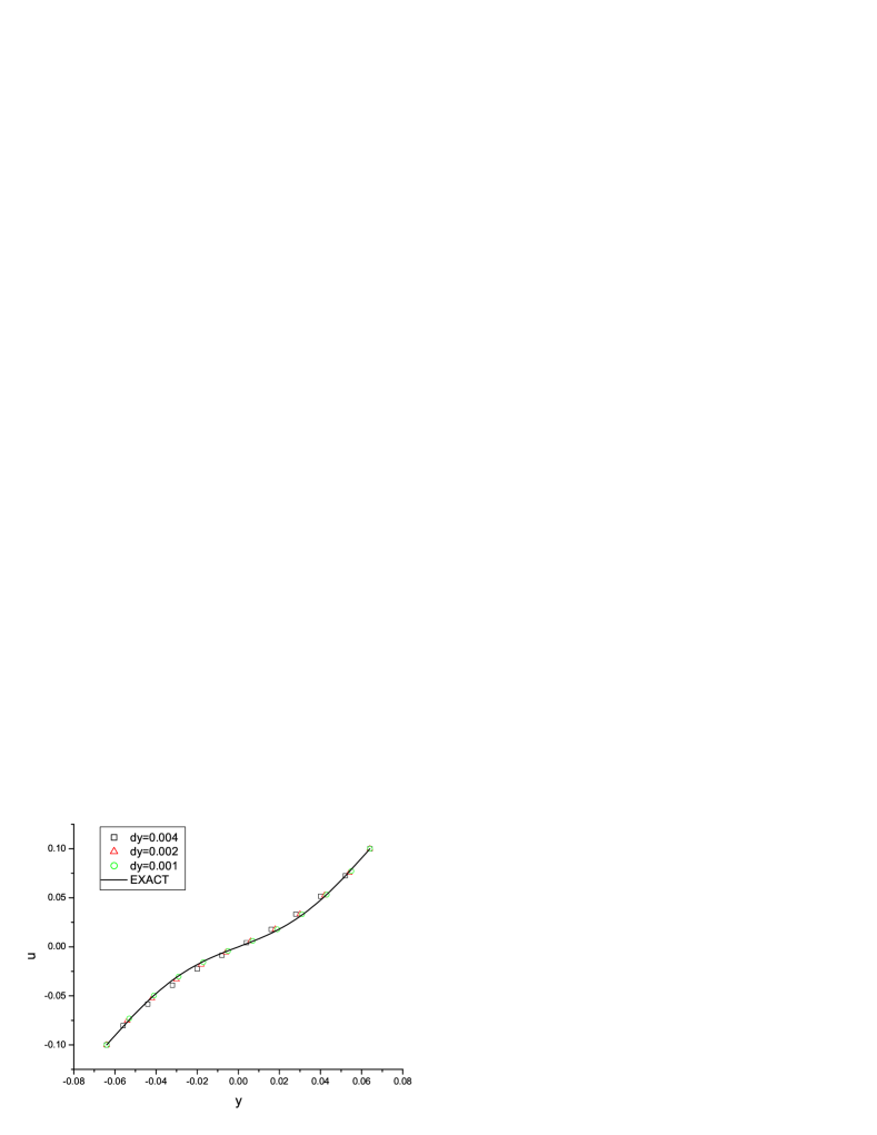
Figure 11: Comparison of the MRT LB simulation results and exact solutions for the horizontal velocity distribution of Couette fiow at time $t=57.5$.

VI Conclusion

An energy-conserving multiple-relaxation-time finite difference lattice Boltzmann model for compressible flows is proposed. This model is based on a 16-discrete-velocity model designed by Kataoka and Tsutahara21a . The collision step is first calculated in the moment space and then mapped back to the velocity space. The moment space and corresponding transformation matrix are constructed according to the group representation theory. Equilibria of the nonconserved moments are chosen according to the need of recovering compressible Navier-Stokes equations through the Chapman-Enskog expansion. In the new model different transport coefficients, such as viscosity and heat conductivity, are related to different collision parameters. Consequently, they can be controlled independently. This flexibility makes the MRT model contain more physical information and easier to satisfy the von Neumann stability condition than its SRT counterpart. The new model passed well-known benchmark tests, including (i) shock tubes, such as the Sod, Lax, Colella explosion wave, collision of two strong shocks and a new shock tube with high Mach number, (ii) regular and Mach shock reflections, (iii) shock wave reaction on cylindrical bubble problems, and (iv) Couette flow. This model works for both low and high speeds compressible flows. Both the LB and traditional CFD approach work when the Knudsen number is very small, but in the vicinity of shock wave, the system is in a nonequilibrium state, and the traditional Euler and Navier-Stokes descriptions are problematic. For such problems, LB has more sound physical ground.

Appendix. Spatial and temporal discretization effects

In our simulations, the time evolution is based on the usual first-order upwind scheme, while space discretization is performed through a Lax-Wendroff scheme.

$$\frac{\partial}{\partial t}f_{i}=[f_{i}(t+\delta t)-f_{i}(t)]/\delta t\text{,}$$ (30a)

$$\overrightarrow{v}_{i}\cdot\nabla f_{i} = v_{ix}[f_{i}(x+\delta x,y)-f_{i}(x-\delta x,y)]/2\delta x$$ (30b)

$$+v_{iy}[f_{i}(x,y+\delta y)-f_{i}(x,y-\delta y)]/2\delta y$$

$$-v_{ix}^{2}\delta t[f_{i}(x+\delta x,y)-2f_{i}(x,y)+f_{i}(x-\delta x,y)]/2\delta x^{2}$$

$$-v_{iy}^{2}\delta t[f_{i}(x,y+\delta y)-2f_{i}(x,y)+f_{i}(x,y-\delta y)]/2\delta y^{2}\text{.}$$

If we perform the following series expansion up to second order in Eq.(30a) and Eq.(30b)

$$f_{i}(t+\delta t)=f_{i}(t)+\delta t\frac{\partial}{\partial t}f_{i}+\frac{1}{2}\delta t^{2}\frac{\partial^{2}}{\partial t^{2}}f_{i}\text{,}$$ (31a)

$$f_{i}(x+\delta x,y,t)=f_{i}(x,y,t)+\delta x\frac{\partial}{\partial x}f_{i}+\frac{1}{2}\delta x^{2}\frac{\partial^{2}}{\partial x^{2}}f_{i}\text{,}$$ (31b)

$$f_{i}(x-\delta x,y,t)=f_{i}(x,y,t)-\delta x\frac{\partial}{\partial x}f_{i}+\frac{1}{2}\delta x^{2}\frac{\partial^{2}}{\partial x^{2}}f_{i}\text{,}$$ (31c)

we can get

$$\frac{\partial}{\partial t}f_{i}\Rightarrow\frac{\partial}{\partial t}f_{i}+\frac{1}{2}\delta t\frac{\partial^{2}}{\partial t^{2}}f_{i}\text{,}$$ (32a)

$$\overrightarrow{v}_{i}\cdot\nabla f_{i}\Rightarrow v_{ix}\frac{\partial}{\partial x}f_{i}+v_{iy}\frac{\partial}{\partial y}f_{i}-\frac{v_{ix}^{2}\delta t}{2}\frac{\partial^{2}}{\partial x^{2}}f_{i}-\frac{v_{iy}^{2}\delta t}{2}\frac{\partial^{2}}{\partial y^{2}}f_{i}\text{,}$$ (32b)

So a more accurate LB equation solved using the updating schemes mentioned above is,

$$\frac{\partial}{\partial t}f_{i}+\frac{1}{2}\delta t\frac{\partial^{2}}{\partial t^{2}}f_{i}+v_{i\beta}\frac{\partial}{\partial r_{\beta}}f_{i}-\frac{1}{2}\delta tv_{i\beta}^{2}\frac{\partial^{2}}{\partial r_{\beta}^{2}}f_{i}=-\mathbf{S}_{ik}\left[f_{k}-f_{k}^{eq}\right]\text{,}$$ (33)

To investigate the effect of the supplementary terms in Eq.(33), a similar Chapman-Enskog expansion procedure may be considered. The zeroth and first order LB equations Eq.(7a), Eq.(7b) remain unchanged when performing the Chapman–Enskog expansion, while the second-order equation (7c) becomes,

$$\frac{\partial}{\partial t_{2}}f_{i}^{(0)}+\frac{\partial}{\partial t_{1}}f_{i}^{(1)}-\frac{\delta t}{2}\frac{\partial}{\partial t_{1}}(\mathbf{S}_{il}f_{l}^{(1)})+v_{i\alpha}\frac{\partial}{\partial x_{1\alpha}}f_{i}^{(1)}+\frac{\delta t}{2}v_{i\alpha}\frac{\partial}{\partial x_{1\alpha}}(\mathbf{S}_{il}f_{l}^{(1)})+{}$$

$$\frac{\delta t}{2}v_{i\alpha}v_{i\beta}\frac{\partial}{\partial x_{1\alpha}}\frac{\partial}{\partial x_{1\beta}}f_{i}^{(0)}-\frac{\delta t}{2}v_{i\alpha}^{2}\frac{\partial^{2}}{\partial x_{1\alpha}^{2}}f_{i}^{(0)}=-\mathbf{S}_{il}f_{l}^{(2)}\text{.}$$ (34)

It can be converted into moment space to obtain:

$$\frac{\partial}{\partial t_{2}}\hat{f}_{i}^{(0)}+\frac{\partial}{\partial t_{1}}\hat{f}_{i}^{(1)}-\frac{\delta t}{2}\frac{\partial}{\partial t_{1}}(\hat{\mathbf{S}}_{il}\hat{f}_{l}^{(1)})+\hat{\mathbf{E}}_{i\alpha}\frac{\partial}{\partial x_{1\alpha}}\hat{f}_{i}^{(1)}+\frac{\delta t}{2}\hat{\mathbf{E}}_{i\alpha}\frac{\partial}{\partial x_{1\alpha}}(\hat{\mathbf{S}}_{il}\hat{f}_{l}^{(1)})+{}$$

$$\frac{\delta t}{2}\hat{\mathbf{E}}_{i\alpha}\hat{\mathbf{E}}_{i\beta}\frac{\partial}{\partial x_{1\alpha}}\frac{\partial}{\partial x_{1\beta}}\hat{f}_{i}^{(0)}-\frac{\delta t}{2}\hat{\mathbf{E}}_{i\alpha}^{2}\frac{\partial^{2}}{\partial x_{1\alpha}^{2}}\hat{f}_{i}^{(0)}=-\hat{\mathbf{S}}_{il}\hat{f}_{l}^{(2)}\text{,}$$ (35)

where $\hat{\mathbf{E}}_{\alpha}=\mathbf{M}(v_{\alpha}\mathbf{I})\mathbf{M}^{-1}$. From the equation, we obtain

$$\frac{\partial\rho}{\partial t_{2}}+\delta t\frac{\partial}{\partial x_{1}}\frac{\partial}{\partial y_{1}}\hat{f}_{6}^{eq}=0\text{,}$$ (36a)

$$\frac{\partial j_{x}}{\partial t_{2}}+\frac{1}{2}\frac{\partial}{\partial x_{1}}(1+\frac{\delta t}{2}s_{5})\hat{f}_{5}^{(1)}+\frac{\partial}{\partial y_{1}}(1+\frac{\delta t}{2}s_{6})\hat{f}_{6}^{(1)}+\frac{\delta t}{4}\frac{\partial}{\partial x_{1}}\frac{\partial}{\partial y_{1}}(\hat{f}_{10}^{eq}+2\hat{f}_{8}^{eq})=0\text{,}$$ (36b)

$$\frac{\partial j_{y}}{\partial t_{2}}+\frac{\partial}{\partial x_{1}}(1+\frac{\delta t}{2}s_{6})\hat{f}_{6}^{(1)}-\frac{1}{2}\frac{\partial}{\partial y_{1}}(1+\frac{\delta t}{2}s_{5})\hat{f}_{5}^{(1)}+\frac{\delta t}{4}\frac{\partial}{\partial x_{1}}\frac{\partial}{\partial y_{1}}(2\hat{f}_{7}^{eq}-\hat{f}_{9}^{eq})=0\text{,}$$ (36c)

$$\frac{\partial e}{\partial t_{2}}+\frac{\partial}{\partial x_{1}}(1+\frac{\delta t}{2}s_{7})\hat{f}_{7}^{(1)}+\frac{\partial}{\partial y_{1}}(1+\frac{\delta t}{2}s_{8})\hat{f}_{8}^{(1)}+\frac{\delta t}{2}\frac{\partial}{\partial x_{1}}\frac{\partial}{\partial y_{1}}\hat{f}_{14}^{eq}=0\text{.}$$ (36d)

In this way the recovered NS equations are as follows:

$$\frac{\partial\rho}{\partial t}+\frac{\partial j_{x}}{\partial x}+\frac{\partial j_{y}}{\partial y}=-\delta t\frac{\partial}{\partial x}\frac{\partial}{\partial y}(j_{x}j_{y}/\rho)\text{,}$$ (37a)

$$\frac{\partial j_{x}}{\partial t}+\frac{\partial}{\partial x}\left(j_{x}^{2}/\rho\right)+\frac{\partial}{\partial y}\left(j_{x}j_{y}/\rho\right)=-\frac{\partial P}{\partial x}+\frac{\partial}{\partial x}[\mu_{s}^{{}^{\prime}}(\frac{\partial u_{x}}{\partial x}-\frac{\partial u_{y}}{\partial y})]+\frac{\partial}{\partial y}[\mu_{v}^{{}^{\prime}}(\frac{\partial u_{y}}{\partial x}+\frac{\partial u_{x}}{\partial y})]-\delta t\frac{\partial}{\partial x}\frac{\partial}{\partial y}[(\rho u_{x}^{2}+P)u_{y}]\text{,}$$ (37b)

$$\frac{\partial j_{y}}{\partial t}+\frac{\partial}{\partial x}\left(j_{x}j_{y}/\rho\right)+\frac{\partial}{\partial y}\left(j_{y}^{2}/\rho\right)=-\frac{\partial P}{\partial y}+\frac{\partial}{\partial x}[\mu_{v}^{{}^{\prime}}(\frac{\partial u_{y}}{\partial x}+\frac{\partial u_{x}}{\partial y})]-\frac{\partial}{\partial y}[\mu_{s}^{{}^{\prime}}(\frac{\partial u_{x}}{\partial x}-\frac{\partial u_{y}}{\partial y})]-\delta t\frac{\partial}{\partial x}\frac{\partial}{\partial y}[(\rho u_{y}^{2}+P)u_{x}]\text{,}$$ (37c)

$$\frac{\partial e}{\partial t}+\frac{\partial}{\partial x}[(e+P)j_{x}/\rho]+\frac{\partial}{\partial y}[(e+P)j_{y}/\rho]$$ (37d)

$$= \frac{\partial}{\partial x}[\lambda_{1}^{{}^{\prime}}(2\frac{\partial T}{\partial x}+u_{y}\frac{\partial u_{y}}{\partial x}+u_{x}\frac{\partial u_{x}}{\partial x}-u_{x}\frac{\partial u_{y}}{\partial y}+u_{y}\frac{\partial u_{x}}{\partial y})]$$

$$+\frac{\partial}{\partial y}[\lambda_{2}^{{}^{\prime}}(2\frac{\partial T}{\partial y}+u_{x}\frac{\partial u_{x}}{\partial y}-u_{y}\frac{\partial u_{x}}{\partial x}+u_{x}\frac{\partial u_{y}}{\partial x}+u_{y}\frac{\partial u_{y}}{\partial y})]$$

$$-\delta t\frac{\partial}{\partial x}\frac{\partial}{\partial y}[(3P+\frac{1}{2}\rho u^{2})u_{x}u_{y}]\text{,}$$

where

$$\mu_{s}^{{}^{\prime}}=\rho RT(\frac{1}{s_{5}}+\frac{\delta t}{2})\text{, }\mu_{v}^{{}^{\prime}}=\rho RT(\frac{1}{s_{6}}+\frac{\delta t}{2})\text{, }\lambda_{1}^{{}^{\prime}}=\rho R^{2}T(\frac{1}{s_{7}}+\frac{\delta t}{2})\text{, }\lambda_{2}^{{}^{\prime}}=\rho R^{2}T(\frac{1}{s_{8}}+\frac{\delta t}{2})\text{.}$$

When $\delta t$ approaches $0$, equations (37a)-(37d) reduce to the Eqs.(13a)-(13d).

References

- (1) B. Chopard and M. Droz, Cellular Automata Modeling of Physical Systems, Cambridge University Press, New York (1998).
- (2) S. Succi, The Lattice Boltzmann Equation for Fluid Dynamics and Beyond,Oxford University Press, New York (2001).
- (3) P. Bhatnagar, E. P. Gross, and M. K. Krook, Phys. Rev. 94, 511 (1954).
- (4) X. Shan, H. Chen, Phys. Rev. E 47, 1815 (1993); Phys. Rev. E 49, 2941 (1994).
- (5) M. R. Swift, W. R. Osborn, J. M. Yeomans, Phys. Rev. Lett. 75, 830 (1995); G. Gonnella, E. Orlandini, and J. M. Yeomans, Phys. Rev. Lett. 78, 1695 (1997); A. J. Wagner and J. M. Yeomans, Rev. Lett. 80, 1429 (1998); D. Marenduzzo, E. Orlandini, and J.M. Yeomans, Phys. Rev. Lett. 92, 188301 (2004); R. Verberg, C.M. Pooley, J.M. Yeomans, and A. C. Balazs, Phys. Rev. Lett. 93,184501(2004); D. Marenduzzo, E. Orlandini, and J. M. Yeomans, Phys. Rev. Lett. 98, 118102 (2007).
- (6) Aiguo Xu, G. Gonnella, A. Lamura, Phys. Rev. E 67, 056105(2003); Phys. Rev. E 74, 011505(2006); Physica A 331, 10(2004); Physica A 344, 750(2004);Physica A 362, 42(2006).
- (7) Aiguo Xu, G. Gonnella, A. Lamura, G. Amati and F. Massaioli, Europhys. Lett. 71, 651 (2005).
- (8) Aiguo Xu, Commun. Theor. Phys. 39, 729(2003).
- (9) Aiguo Xu, S. Succi, B. M. Boghosiand, Math. & Comput. Simulat. 72, 249 (2006).
- (10) M. Sbragaglia, R. Benzi, L. Biferale, S. Succi, K. Sugiyama, and F. Toschi, Phys. Rev. E 75, 026702 (2007).
- (11) C. Wang, Aiguo Xu, Guangcai Zhang, Y. Li, Sci. China Ser. G-Phys. Mech. Astron. 52, 1337(2009).
- (12) S. Chen, H. Chen, D. Martinez, W. Matthaeus, Phys. Rev. Lett. 67, 3776 (1991).
- (13) D. O. Martinez, S. Chen,and W. H. Matthaeus, Phys. Plasmas 1, 1850 (1994).
- (14) V. Sofonea and W. G. Fruh, Eur. Phys. J. B, 20, 141 (2001).
- (15) S. Succi, M. Vergassola and R. Benzi, Phys. Rev. A 43, 4521 (1991).
- (16) W. Schaffenberger and A. Hanslmeier, Phys. Rev. E 66, 046702 (2002).
- (17) G. Breyiannis and D. Valougeorgis, Phys. Rev. E 69, 065702(R) (2004).
- (18) G. Vahala, B. Keating,M. Soe, J. Yepez, L. Vahala, J. Carter and S. Ziegeler, Commun. Comput. Phys. 4, 624 (2008).
- (19) D. H. Rothman, Geophysics, 53, 509 (1988).
- (20) A. Gunstensen and D. H. Rothman, J. Geophy. Research, 98, 6431 (1993).
- (21) Q. J. Kang, D. X. Zhang, S. Y. Chen, Phys. Rev. E 66, 056307 (2002).
- (22) F. J. Alexander, S. Chen, and J. D. Sterling, Phys. Rev. E 47, R2249 (1993).
- (23) Y. Qian, J. Sci. Comp. 8, 231 (1993).
- (24) Y. Chen, H. Ohashi, and M. Akiyama, J. Sci. Comp. 12, 169 (1997).
- (25) F. J. Higuera, S. Succi and R. Benzi, Europhys. Lett., 9, 345 (1989). F. J. Higuera and J. Jimenez, Europhys. Lett., 9, 662, (1989).
- (26) D. d’Humières, Generalized lattice-Boltzmann equations, in Rarefied Gas Dynamics: Theory and Simulations, edited by B. D. Shizgal and D. P Weaver, Progress in Astronautics and Aeronautics, Vol. 159(AIAA Press, Washington, DC, 1992), pp450-458.
- (27) P. Lallemand, and L. S. Luo, Phys. Rev. E 61, 6546 (2000).
- (28) P. Lallemand, and L. S. Luo, Phys. Rev. E 68, 036706 (2003).
- (29) L. Giraud, D. d’Humières, and P. Lallemand, Int. J. Mod. Phys. C 8, 805 (1997).
- (30) L. Giraud, D. d’Humières, and P. Lallemand, Europhys. Lett. 42, 625 (1998).
- (31) P. Lallemand, D. d’Humières, L. S. Luo and R. Rubinstein, Phys. Rev. E 67, 021203 (2003).
- (32) M. E. McCracken, and J. Abraham, Phys. Rev. E 71, 036701 (2005).
- (33) K. N. Premnath, and J. Abraham, J. Comp. Phys. 224, 539 (2007).
- (34) I. Ginzburg, and K. Steiner, Phil. Trans. R. Soc. Lond. A 360, 453 (2002).
- (35) I. Ginzbourg, and P. M. Adler, J. Physique II 4, 191 (1994).
- (36) F. J. Alexander, H. Chen, S. Chen and G. D. Doolen, Phys. Rev. A 46, 1967 (1992).
- (37) Y. X. Li ,L. S. Kang and Z. J. Wu, Neural Parallel Sci. Comput., 1, 43 (1993).
- (38) C. H. Sun, Phys Rev E 58, 7283 (1998); C. Sun and A. T. Hsu, Phys. Rev. E 68, 016303 (2003).
- (39) G. W. Yan, Y. S. Chen, S. X. Hu. Phys Rev E 59, 454 (1999).
- (40) M. Watari and M. Tsutahara, Phys. Rev. E 67, 036306 (2003); Phys. Rev. E 70, 016703 (2004).
- (41) T. Kataoka and M. Tsutahara, Phys. Rev. E 69, 035701(R) (2004); Phys. Rev. E 69, 056702 (2004).
- (42) Aiguo Xu, Europhys. Lett. 69, 214 (2005); Phys Rev E 71, 066706 (2005); Progr. Theore. Phys.(Suppl.) 162, 197 (2006).
- (43) F. Tosi, S. Ubertini, S. Succi, H. Chen, I.V. Karlin, Math. Comput. Simul. 72, 227(2006).
- (44) S. Ansumali, I.V. Karlin, J. Stat. Phys. 107, 291(2002).
- (45) Y. Li, R. Shock, R. Zhang, H. Chen, J. Fluid Mech. 519, 273(2004) .
- (46) V. Sofonea, A. Lamura, G. Gonnella, A. Cristea, Phys. Rev. E 70, 046702 (2004).
- (47) X.F.Pan, Aiguo Xu, Guangcai Zhang, S. Jiang, Int. J. Mod. Phys. C 18, 1747 (2007); Y. Gan, Aiguo Xu, Guangcai Zhang, X. Yu, Y. Li, Physica A 387, 1721 (2008).
- (48) R. A. Brownlee, A. N. Gorban, J. Levesley, Phys. Rev. E 75, 036711 (2007).
- (49) S. Chapman and T.G. Cowling, The mathematical theory of non-uniform gases, Cambridge University Press, London (1970).
- (50) R. Du, B. Shi, X. Chen, Phys. Lett. A 359,564 (2006).
- (51) K. Xu, L. Martinelli, and A. Jameson, J. Comput. Phys. 120, 48 (1995).
- (52) P. Colella, J. Comput. Phys. 87, 171 (1990).
- (53) K. Qu, C. Shu, and Y. T. Chew, Phys. Rev. E 75, 036706(2007).
- (54) C. Q. Jin, K. Xu, J. Comput. Phys. 218, 68 (2006).
- (55) J. F. Haas and B. Sturtevant, J. Fluid Mech. 181, 41 (1987).