Two–dimensional Anderson–Hubbard model in DMFT+$\Sigma$ approximation.

Abstract

Density of states, dynamic (optical) conductivity and phase diagram of paramagnetic two – dimensional Anderson – Hubbard model with strong correlations and disorder are analyzed within the generalized dynamical mean field theory (DMFT+$\Sigma$ approximation). Strong correlations are accounted by DMFT, while disorder is taken into account via the appropriate generalization of the self – consistent theory of localization. We consider the two – dimensional system with the rectangular “bare” density of states (DOS). The DMFT effective single impurity problem is solved by numerical renormalization group (NRG). Phases of “correlated metal”, Mott insulator and correlated Anderson insulator are identified from the evolution of density of states, optical conductivity and localization length, demonstrating both Mott – Hubbard and Anderson metal – insulator transitions in two – dimensional systems of the finite size, allowing us to construct the complete zero – temperature phase diagram of paramagnetic Anderson – Hubbard model. Localization length in our approximation is practically independent of the strength of Hubbard correlations. However, the divergence of localization length in finite size two – dimensional system at small disorder signifies the existence of an effective Anderson transition.

I Introduction

The study of disordered electronic systems with the account of interaction effects belongs to the central problems of the modern condensed matter theory Lee85 . According to the scaling theory of localization AALR79 there is no metallic state in two – dimensional (2D) systems, all electronic states are localized at the smallest possible disorder. This prediction was made first for noninteracting 2D systems, soon after it was shown that the weak electron – electron interaction in most cases enhance localization AAL80 . Experiments performed in early 80’s on different 2D systems 2Dexp essentially confirmed these predictions. However, some theoretical works produced an evidence of rather different possibility ma for 2D systems to evolve to the state with even infinite metallic – like conductivity at zero temperature ($T=0$) in case of weak disorder and sufficiently strong correlations. Experimental observation of metal – insulator transition (MIT) in 2D systems with weak enough disorder but strong correlations (low electronic densities) Krav04 , which apparently contradicted the predictions of the scaling theory of localization, stimulated extensive theoretical studies with no widely accepted solution up to now (see the review in Ref. AKS01, ).

One of the basic models allowing for the simultaneous account of both strong enough electronic correlations, leading to Mott MIT transition Mott90 , and effects of strong disorder, leading to Anderson MIT Anderson58 , is the Anderson – Hubbard model, intensively studied in recent years Dobrosavljevic97 ; Dobrosavljevic03 ; BV ; HubDis ; ShapiroPRB08 ; Shapiro08 ; PB09 .

In Refs. Dobrosavljevic97 ; Dobrosavljevic03 ; BV three – dimensional (3D) Anderson – Hubbard model was analyzed with dynamical mean field theory (DMFT), which is extensively used in the theory of strongly correlated electrons MetzVoll89 ; vollha93 ; pruschke ; georges96 . However, disorder effects were mostly taken into account via the average density of states and the coherent potential approximation (CPA) ulmke95 ; vlaming92 , which misses the effects of Anderson localization. To overcome this problem Dobrosavljević and Kotliar Dobrosavljevic97 have proposed the DMFT approach, where the solution of self – consistent stochastic DMFT equations were used to calculate geometrically averaged local density of states. This approach was further developed in Refs. Dobrosavljevic03 ; BV with DMFT account for Hubbard correlations, which leads to highly nontrivial phase diagram of 3D paramagnetic Anderson – Hubbard model BV , containing the phases of correlated metal, Mott insulator and correlated Anderson insulator. However, the major problem of the approach of Refs. Dobrosavljevic97 ; Dobrosavljevic03 ; BV is its practical inability of direct calculations of conductivity, which actually determines MIT itself.

In the previous work HubDis we have studied the 3D paramagnetic Anderson – Hubbard model using our recently developed DMFT+$\Sigma$ approximation JTL05 ; PRB05 ; FNT06 ; PRB07 , which conserves the standard single impurity DMFT approach, taking into account the local Hubbard correlations, allowing the use the usual “ impurity solvers” like NRG NRG ; BPH ; Bull , at the same time allowing to include additional (local or nonlocal) interactions. Strong disorder was accounted via some generalization of the self – consistent theory of localization VW ; WV ; MS ; MS86 ; VW92 ; Diagr . In the framework of this approach we have been able not only to reproduce the phase diagram qualitatively similar to that obtained in Ref. BV, , but also calculate the dynamic (optical) conductivity for the wide frequency range.

In Ref. Shapiro08, the Hubbard – Anderson model was studied both for 3D and 2D systems. As the main mechanism leading to delocalization a kind of “screening” of the random (disorder) potential by local Hubbard interaction was introduced ShapiroPRB08 . Then the Anderson – Hubbard model was reduced to an effective single – particle Anderson model with renormalized distribution of local site energies, which was calculated in the atomic limit. All the other effects of electronic correlations were neglected. Strong disorder effects were accounted within self – consistent theory of localization. In this approach the authors obtained the significant growth of localization length with growing Hubbard interaction in 2D. However, localization length itself remained finite, the system being localized at smallest possible disorder, so that Anderson in 2D is still absent. Similar result was obtained also in numerical simulations of 2D Anderson – Hubbard model in Ref. PB09, .

In this work we present a direct generalization of the method used in Ref. HubDis, to the case of 2D systems. We use the DMFT+$\Sigma$ approach to calculate DOS, optical conductivity, localization length and construct the phase diagram of 2D paramagnetic Anderson – Hubbard model with strong electronic correlations and strong disorder. Strong correlations are taken into account via DMFT, while disorder effects are treated by the appropriate generalization of the self – consistent theory localization.

The paper is organized as follows: in section II we present a brief description of our DMFT+$\Sigma$ approximation as applied to disordered Hubbard model. In section III we formulate the basic DMFT+$\Sigma$ expressions for optical conductivity and self – consistency equation for the generalizes diffusion coefficient. Our results for DOS, optical conductivity and localization length are given in section IV, where we also analyze the phase diagram of 2D disordered Hubbard model and briefly discuss the optical sum rule within our approach. Finally we present a short conclusion, which includes the discussion of problems yet to be solved.

II Basics of DMFT+$\Sigma$ approach.

In the following we consider paramagnetic disordered Anderson – Hubbard model at half – filling for arbitrary correlations and disorder. This model treats both Mott – Hubbard and Anderson MIT on the same footing. The Hamiltonian of the model can be written as:

$$H=-t\sum_{\langle ij\rangle\sigma}a_{i\sigma}^{\dagger}a_{j\sigma}+\sum_{i\sigma}\epsilon_{i}n_{i\sigma}+U\sum_{i}n_{i\uparrow}n_{i\downarrow},$$ (1)

where $t>0$ is nearest neighbor transfer integral, $U$ is the local Hubbard repulsion, $n_{i\sigma}=a_{i\sigma}^{\dagger}a_{i\sigma}$ is electron number operator at a given site $i$, $a_{i\sigma}$ ($a_{i\sigma}^{\dagger}$) is annihilation (creation) operator for an electron with spin $\sigma$, local energies $\epsilon_{i}$ are assumed to be randomly and independently distributed on different lattice sites. To simplify diagram technique in the following we assume $\epsilon_{i}$ distribution to be Gaussian:

$$\mathcal{P}(\epsilon_{i})=\frac{1}{\sqrt{2\pi}\Delta}\exp\left(-\frac{\epsilon_{i}^{2}}{2\Delta^{2}}\right)$$ (2)

Here $\Delta$ serves as disorder parameter and Gaussian random field (“white” noise) of energy levels $\epsilon_{i}$ at different lattice sites induces “impurity” – like scattering, leading to the standard diagram technique for calculations of the averaged Green’s functions Diagr .

DMDF+$\Sigma$ approach, initially proposed in Refs. JTL05 ; PRB05 ; FNT06 ; PRB07 as a simple method to include nonlocal interactions (fluctuations) into the standard (local) DMFT scheme, is also very convenient for the account in DMFT of any additional interaction (local or nonlocal) of arbitrary nature.

In DMFT+$\Sigma$ approximation we choose the single – particle Green’s function in the following form:

$$G_{\bf p}(\varepsilon)=\frac{1}{\varepsilon+\mu-\varepsilon({\bf p})-\Sigma(\varepsilon)-\Sigma_{\bf p}(\varepsilon)},$$ (3)

where $\varepsilon({\bf p})$ is the “bare” electron spectrum, $\Sigma(\varepsilon)$ is the local (DMFT) self – energy due to Hubbard interactions, while $\Sigma_{\bf p}(\varepsilon)$ is an “external” (in general case momentum dependent) self – energy due to some other interaction. The main assumption of our approach (both its advantage and deficiency) is precisely in this additive form (neglect of interference effects) for the total self – energy in (3) JTL05 ; PRB05 ; FNT06 ; PRB07 , which allows us to conserve the standard form of self – consistent DMFT equations georges96 with two major generalizations. First of all, at each iteration of DMFT – loop we recalculate an “external” self – energy $\Sigma_{\bf p}(\mu,\varepsilon,[G_{\bf p}(\varepsilon)])$ within some (approximate) scheme, taking into account the “external” interaction (in the present case that due to disorder scattering). Secondly, the local Green’s function for an effective DMFT – impurity problem is defined as:

$$G_{ii}(\varepsilon)=\frac{1}{N}\sum_{\bf p}\frac{1}{\varepsilon+\mu-\varepsilon({\bf p})-\Sigma(\varepsilon)-\Sigma_{\bf p}(\varepsilon)},$$ (4)

at each step of the standard DMFT procedure. Finally we obtain the desired Green’s function in the form of Eq. (3), where $\Sigma(\varepsilon)$ and $\Sigma_{\bf p}(\varepsilon)$ are self – energies obtained at the end of our iteration procedure.

For $\Sigma_{\bf p}(\varepsilon)$ appearing due to disorder scattering we shall use the simple one – loop contribution, neglecting diagrams with “crossing” interaction lines, i.e. self – consistent Born approximation Diagr , which in the case of Gaussian disorder (2) leads to the usual expression:

$$\Sigma_{\bf p}(\varepsilon)=\Delta^{2}\sum_{\bf p}G(\varepsilon,{\bf p})\equiv\Sigma_{imp}(\varepsilon)$$ (5)

and “external” self – energy in this case is ${\bf p}$-independent (local).

III Optical conductivity in DMFT+$\Sigma$ approach.

It is obvious that calculations of optical (dynamic) conductivity provide the direct way to study MIT as frequency dependence of conductivity, as well as its static value at zero frequency of an external field, allows the clear distinction between metallic and insulating phases (at temperature $T=0$ ).

Local nature of irreducible self – energy in DMFT allows to reduce the problem of calculation of optical conductivity to calculation of the usual particle – hole loop without DMFT vertex corrections due to local Hubbard interaction PRB07 ; HubDis . The final expression for the real part of optical conductivity obtained in this way in Refs. PRB07 ; HubDis , takes the following form:

$${\rm{Re}}\sigma(\omega)=\frac{e^{2}\omega}{2\pi}\int_{-\infty}^{\infty}d\varepsilon\left[f(\varepsilon_{-})-f(\varepsilon_{+})\right]\times$$

$$\times{\rm{Re}}\left\{\phi^{0RA}_{\varepsilon}(\omega)\left[1-\frac{\Sigma^{R}(\varepsilon_{+})-\Sigma^{A}(\varepsilon_{-})}{\omega}\right]^{2}-\right.$$

$$\left.-\phi^{0RR}_{\varepsilon}(\omega)\left[1-\frac{\Sigma^{R}(\varepsilon_{+})-\Sigma^{R}(\varepsilon_{-})}{\omega}\right]^{2}\right\},$$ (6)

Here $f(\varepsilon)$ is Fermi distribution, $\varepsilon_{\pm}=\varepsilon\pm\frac{\omega}{2}$ and

$$\phi^{0RR(RA)}_{\varepsilon}(\omega)=\lim_{q\to 0}\frac{\Phi^{0RR(RA)}_{\varepsilon}(\omega,{\bf q})-\Phi^{0RR(RA)}_{\varepsilon}(\omega,0)}{q^{2}},$$ (7)

where we have introduced two – particle loops:

$$\Phi^{0RR(RA)}_{\varepsilon}(\omega,{\bf q})=\sum_{\bf p}G^{R}(\varepsilon_{+},{\bf p_{+}})G^{R(A)}(\varepsilon_{-},{\bf p_{-}})$$

$$\Gamma^{RR(RA)}(\varepsilon_{-},{\bf p}_{-};\varepsilon_{+},{\bf p}_{+}),$$ (8)

represented diagrammatically in Fig. 1 with ${\bf p}_{\pm}={\bf p}\pm\frac{\bf q}{2}$ and $R$ and $A$ indices corresponding to retarded and advanced Green’s functions. The vertices $\Gamma^{RR(RA)}(\varepsilon_{-},{\bf p}_{-};\varepsilon_{+},{\bf p}_{+})$ contain all vertex corrections due to disorder scattering, but do not include vertex corrections due to Hubbard interaction.

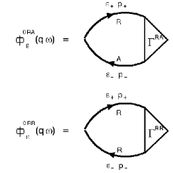
Figure 1: Diagrammatic representation of $\Phi^{0RA}_{\varepsilon}(\omega,{\bf q})$ $\Phi^{0RR}_{\varepsilon}(\omega,{\bf q})$.

Thus, the problem is much simplified. To calculate optical conductivity in DMFT+$\Sigma$ approximation we have only to solve single – particle problem to determine the local self – energy $\Sigma(\varepsilon_{\pm})$ with the help of DMFT+$\Sigma$ procedure, described above, while the nontrivial contribution of disorder scattering enters via $\phi^{0RR(RA)}$ of Eq. (7), which may be calculated in some appropriate approximation. In fact, $\phi^{0RR(RA)}$ contain only disorder scattering, though using as the “bare” the Green’s functions including the DMFT self – energies, already determined with the help of DMFT+$\Sigma$ procedure. Eq. (6) guarantees the effective interpolation between the case of strong correlations in the absence of disorder and the case of pure disorder in the absence of Hubbard correlations.

The most important $\Phi^{0RA}_{\varepsilon}(\omega,{\bf q})$ loop may be calculated using the basic approach of the self – consistent theory of localization VW ; WV ; MS ; MS86 ; VW92 ; Diagr with some generalizations accounting for Hubbard interaction within the DMFT+$\Sigma$ approach HubDis .

The rest is the direct generalization of the scheme proposed in Ref. HubDis, for the two – dimensional case. Here we present only some basic points of the approach of Ref. HubDis, , stressing important differences due to two – dimensionality of the model.

In RA-channel the two – particle loop $\Phi^{0RA}_{\varepsilon}({\bf q},\tilde{\omega})$ possesses a diffusion – like contribution:

$$\Phi^{0RA}_{\varepsilon}({\bf q},\tilde{\omega})=\frac{-\sum_{\bf p}\Delta G_{\bf p}}{\tilde{\omega}+iD(\omega)q^{2}},$$ (9)

where $\Delta G_{\bf p}=G^{R}(\varepsilon_{+},{\bf p})-G^{A}(\varepsilon_{-},{\bf p})$. The important difference with noninteracting case is contained in

$$\tilde{\omega}=\varepsilon_{+}-\varepsilon_{-}-\Sigma^{R}(\varepsilon_{+})+\Sigma^{A}(\varepsilon_{-})=$$

$$\omega-\Sigma^{R}(\varepsilon_{+})+\Sigma^{A}(\varepsilon_{-})\equiv\omega-\Delta\Sigma^{RA}(\omega)$$ (10)

which replaces the usual $\omega$-term in the denominator of the standard expression for $\Phi^{0RA}_{\varepsilon}(\omega,{\bf q})$ Diagr .

Then (6) can be rewritten as:

$${\rm{Re}}\sigma(\omega)=\frac{e^{2}\omega}{2\pi}\int_{-\infty}^{\infty}d\varepsilon\left[f(\varepsilon_{-})-f(\varepsilon_{+})\right]\times$$

$$\times{\rm Re}\left\{\frac{i\sum_{\bf p}\Delta G_{\bf p}D(\omega)}{\omega^{2}}-\phi^{0RR}_{\varepsilon}(\omega)\left[1-\frac{\Delta\Sigma^{RR}(\omega)}{\omega}\right]^{2}\right\}$$

(11)

The second term in (11), which is actually irrelevant at small $\omega$, can be obtained from (7) calculating $\Phi^{0RR}_{\varepsilon}(\omega,{\bf q})$ in the usual “ladder” approximation.

Repeating the derivation scheme of the self – consistent theory of localization presented in Ref. HubDis, , we obtain the following equation for the generalized diffusion coefficient:

$$D(\omega)=i\frac{<v>^{2}}{d}\left\{\tilde{\omega}-\Delta\Sigma_{imp}^{RA}(\omega)\right.+$$

$$\left.+\Delta^{4}\sum_{\bf p}(\Delta G_{\bf p})^{2}\sum_{\bf q}\frac{1}{\tilde{\omega}+iD(\omega)q^{2}}\right\}^{-1},$$ (12)

where $d=2$ is spatial dimension and $\Delta\Sigma^{RA}_{imp}(\omega)=\Sigma_{imp}^{R}(\varepsilon_{+})-\Sigma_{imp}^{A}(\varepsilon_{-})$ is determined by disorder scattering. The average velocity $<v>$, well approximated by Fermi velocity, is defined as:

$$<v>=\frac{\sum_{\bf p}|{\bf v}_{\bf p}|\Delta G_{\bf p}}{\sum_{\bf p}\Delta G_{\bf p}};\\ \ {\bf v}_{\bf p}=\frac{\partial\epsilon({\bf p})}{\partial{\bf p}},$$ (13)

Due to the limits of diffusion approximation summation over $q$ in (12) should be limited by MS86 ; Diagr :

$$q<k_{0}=Min\{l^{-1},p_{F}\}$$ (14)

where $l=<v>/2\gamma$ is the mean – free path due to elastic scattering ($\gamma$ is the scattering rate due to disorder), $p_{F}$ is Fermi momentum. In our two – dimensional model Anderson localization takes place at infinetisimal disorder. However, for small disorder localization length is exponentially large, so that the size of the sample becomes important. The sample size $L$ may be introduced into the self – consistent theory of localization as a cutoff of diffusion pole contribution at small $q$ VW ; WV , i.e. for:

$$q\sim k_{L}=1/L.$$ (15)

Eq. (12) for the generalized diffusion coefficient reduces to a transcendental equation, which is easily solved by iterations for each value of $\tilde{\omega}$, taking into account that for $d=2$ and cutoffs defined by Eqs. (14), (15) the sum over $q$ in (12) reduces to:

$$\sum_{\bf q}\frac{1}{\tilde{\omega}+iD(\omega)q^{2}}=\frac{1}{i2\pi D(\omega)}\int_{\frac{k_{L}}{k_{0}}}^{1}\frac{ydy}{y^{2}+\frac{\tilde{\omega}}{iD(\omega)k_{0}^{2}}}=$$ (16)

$$=\frac{1}{i4\pi D(\omega)}\ln{\left(\frac{1-\frac{i\tilde{\omega}}{D(\omega)k_{0}^{2}}}{(\frac{k_{L}}{k_{0}})^{2}-\frac{i\tilde{\omega}}{D(\omega)k_{0}^{2}}}\right)}\\$$

Solving Eq. (12) for different values of our model parameters and using Eq. (11) we can directly calculate the optical (dynamic) conductivity in different phases of the Anderson – Hubbard model.

For $\omega\rightarrow 0$ (and at the Fermi level ($\varepsilon=0$) obviously also $\tilde{\omega}\rightarrow 0$), in Anderson insulator phase we obtain the localization behavior of the generalized diffusion coefficient VW ; WV ; Diagr :

$$D(\omega)=-i\tilde{\omega}{R_{loc}}^{2}.$$ (17)

After the substitution of (17) into (12) we get an equation, determining the localization length $R_{loc}$:

$${R_{loc}}^{2}=-\frac{<v>^{2}}{d\Delta^{4}}\left\{\sum_{\bf p}(\Delta G_{\bf p})^{2}\sum_{\bf q}\frac{1}{1+{R_{loc}}^{2}q^{2}}\right\}^{-1}.$$ (18)

where the sum over $q$ is defined by (16). As we shall see in the following, for an infinite two – dimensional system ($L\to\infty$) localization length, determined by Eq. (18) remains finite (though exponentially large) for the smallest possible disorder, signifying the absence of Anderson transition. However, for the finite size systems localization length diverges at some critical disorder, determined for each value of the system size $L$. Qualitatively, this critical disorder is determined from the condition of localization length (in infinite system) becoming of the order of characteristic sample size $R_{loc}^{L\to\infty}\sim L$. Thus, in finite two – dimensional systems the Anderson transition and metallic phase do exist for disorder strength lower, than this critical disorder. In the following, this kind of metallic phase will be referred to as a phase of the “correlated metal” in finite 2D systems.

IV Main results

Below we present the results of extensive numerical calculations for 2D Anderson – Hubbard model on the square lattice with rectangular “bare” DOS, corresponding to the bandwidth $W=2D$:

$$N_{0}(\varepsilon)=\left\{\begin{array}[]{ll}\frac{1}{2D}&\quad|\varepsilon|\leq D\\ 0&\quad|\varepsilon|>D\end{array}.\right.$$ (19)

The choice of this model DOS is dictated by its 2D nature.

Everywhere below we give the values of DOS in units of the number of states per energy interval, per lattice cell of the volume $a^{2}$ ($a$ – lattice parameter), per one spin projection.

As we concentrate on half – filled case, Fermi level is always assumed to be at zero energy.

As “impurity solver” for DMFT effective impurity problem we have used the reliable numerical renormalization group (NRG) approach NRG ; BPH ; Bull . Calculations were made for low enough temperature $T\sim 0.001D$, so that temperature effects in DOS and conductivity are just negligible.

Now we present only most typical results.

IV.1 Evolution of the density of states

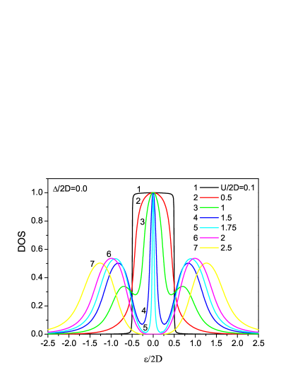
Figure 2: Density of states of the half – filled Anderson – Hubbard model for different values of $U$ and $\Delta=0$ (no disorder).

In Fig. 2 we show evolution of the DOS with the growth of Hubbard interaction $U$ in the absence of disorder. At small $U$ (curve 1 in Fig.2) we observe practically rectangular DOS almost coinciding with the “bare” one. As $U$ grows a typical three peak structure of DOS appears pruschke ; georges96 ; Bull (curves 3,4,5 in Fig.2): a narrow quasiparticle peak at the Fermi level with upper and lower Hubbard bands at $\varepsilon\sim\pm U/2$. Quasiparticle peak narrows as $U$ grows in metallic phase, disappearing at Mott MIT for $U=U_{c2}\approx 1.83W$. With further growth of $U$ (curves 6,7 in Fig.2) dielectric gap opens at the Fermi level.

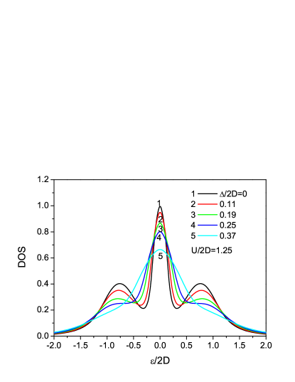
Figure 3: Density of states of the half – filled Anderson – Hubbard model for different values of disorder $\Delta$ and $U/2D=1.25$, typical for correlated metal (in the absence of disorder).

In Fig. 3 we show the results for DOS obtained at relatively weak correlation strength $U=1.25W$ ($W=2D$), so that the system is rather far fron the Mott transition, but for the wide range of disorder strength $\Delta$. We observe typical widening of the band with appropriate suppression of DOS as disorder grows.

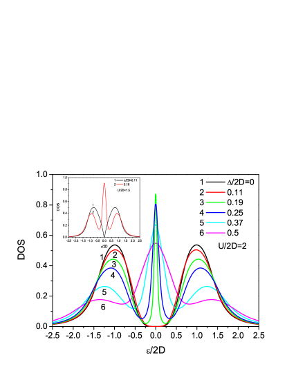
Figure 4: Density of states of the half – filled Anderson – Hubbard model for different values of disorder $\Delta$ and $U/2D=2$, typical for Mott insulator (in the absence of disorder). At the insert – restoration of quasiparticle band by disorder in coexistence (hysteresis) region for $U=1.5D$, obtained from Mott insulator with decreasing $U$.

In Fig. 4 DOS evolution is shown as disorder $\Delta$ grows at $U=2W$, typical for Mott insulator in the absence of disorder. It can be seen that the growth of disorder leads to restoration of the quasiparticle peak in DOS. Similar unusual behavior of DOS (closing of dielectric gap by disorder) was first noted in 3D systems HubDis . However, in the present 2D case it does not, in general, signify the transition to the correlated metal phase, at least for the infinite systems we are, in fact, dealing with correlated Anderson insulator (cf. below).

The physical reason for this unusual restoration of the quasiparticle peak in DOS is clear. Controlling parameter for appearance or disappearance of quasiparticle peak in DMFT in the absence of disorder is the ratio of Hubbard interaction $U$ and the “bare” bandwidth $W=2D$. Disordering leads to the growth of the effective bandwidth $W_{eff}$ (in the absence of Hubbard interaction) and appropriate suppression of $U/W_{eff}$ ratio, which obviously leads to the restoration of quasiparticle band in our model. In more details this qualitative picture will be discussed in Section IV.3, where our results for DOS will be used in construction of the phase diagram of 2D Anderson – Hubbard model.

It is well known, that hysteresis behavior of DOS is obtained for Mott–Hubbard transition if we perform DMFT calculations with $U$ decreasing from insulating phase georges96 ; Bull . Mott insulator phase survives for the values of $U$ well inside the correlated metal phase, obtained with the increase of $U$. Metallic phase is restored at $U_{c1}\approx 1.42W$. The values of $U$ from the interval $U_{c1}<U<U_{c2}$ are usually considered as belonging to coexistence region of metallic and (Mott) insulating phases, with metallic phase being thermodynamically more stable georges96 ; Bull . In the coexistence region disorder increase also leads to the restoration of quasiparticle peak in the DOS (see insert of Fig.4).

IV.2 Optical conductivity: Mott – Hubbard and Anderson transitions.

The real part of optical conductivity was calculated for different combinations of parameters of the model, directly from Eqs. (11) and (12), using the results of DMFT+$\Sigma$ procedure for single – particle characteristics. The values of conductivity below are given in natural units of ${e^{2}}/{\hbar}$.

In the absence of disorder we just reproduce the results of the standard DMFT with optical conductivity characterized by the usual Drude peak at zero frequency and a wide maximum at $\omega\sim U$, corresponding to transitions to the upper Hubbard band. As $U$ grows Drude peak is suppressed and disappear at Mott MIT, when only remaining contribution is due to transitions through the Mott – Hubbard gap.

Introduction of disorder leads to qualitative change of frequency behavior of conductivity. Below we mainly present results obtained for the same values of $U$ and $\Delta$, which were used above to illustrate evolution of DOS.

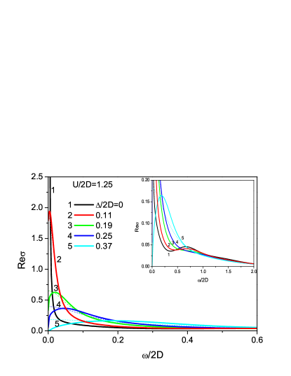
Figure 5: Real part of dynamic conductivity of the half – filled Anderson – Hubbard model for different values of disorder $\Delta$ and $U/2D=1.25$, typical for correlated metal (in the absence of disorder). At the insert – the same, but in wider frequency range. Thin dashed lines represent the results of ladder approximation.

In Fig. 5 we show the real part of optical conductivity in 2D half – filled Anderson – Hubbard model for different disorder strengths $\Delta$ and $U=1.25W$, when the system is far from Mott MIT. Thin dashed lines in Fig. 5 (as well as in the following figures) we show the results of the “ladder” approximation. In 2D model under consideration conductivity at zero frequency is always zero, and in contrast to 3D case HubDis , even for the weakest possible disorder the peak in optical conductivity is at finite frequency. In the “ladder” approximation, which does not contain localization corrections, conductivity at $\omega=0$ is finite. Optical transitions to the upper Hubbard band at $\omega\sim U$ are practically unobservable in these data, only at the insert in Fig. 5, where we show the data for the wide frequency range, we can observe some weak maximum on curves 1 and 2, corresponding to transitions to the upper Hubbard band.

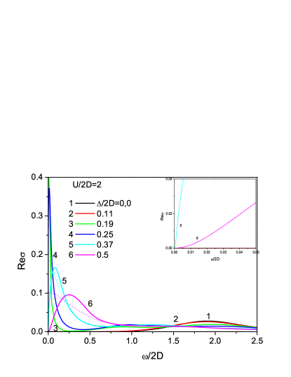
Figure 6: Real part of dynamic conductivity of the half – filled Anderson – Hubbard model for different values of disorder $\Delta$ and $U/2D=2$, typical for Mott insulator (in the absence of disorder). Curves 1,2 correspond to Mott insulator, while curves 3-6 correspond to correlated Anderson insulator. At the insert – localization behavior of conductivity. Thin dashed lines – ladder approximation.

In Fig. 6 we present the real part of optical conductivity for different disorder strengths $\Delta$ and $U=2W$, typical for Mott insulator. It can be seen from Fig. 6 that for small disorder we are in Mott insulator phase (curves 1,2), and with the growth of disorder in the absence of Anderson localization (cf. thin lines corresponding to “ladder” approximation) we would be entering the metallic phase. However, in our model localization takes place at infinetesimal disorder and we are actually entering Anderson insulator phase, with conductivity going to zero at zero frequency. Data in the frequency range corresponding to localization behavior of conductivity $\sigma(\omega)\sim{\omega}^{2}$ are shown at the insert in Fig. 6 for curve 5 and 6, corresponding to large enough disorder. At small disorders the frequency region with localization behavior of conductivity is exponentially small (which is due to the exponential growth of localization length at small disorder, cf. Fig.9) and is practically unobservable.

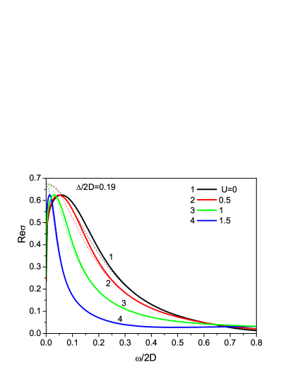
Figure 7: Real part of dynamic conductivity of the half – filled Anderson – Hubbard model for different values of $U$ and $\Delta/2D=0.19$. Thin dashed lines – ladder approximation.

Dependence of optical conductivity on $U$ is illustrated in Fig. 7. The growth of $U$ shifts localization peak in conductivity to lower frequencies and leads to its narrowing. Apparently this is related to the appropriate suppression of quasiparticle peak width in DOS. The value of conductivity at the maximum is $U$ independent. It is interesting to note that for frequencies larger than the maximum position the growth of $U$ suppresses conductivity, while for the frequencies lower than the maximum position the growth of $U$ enhances conductivity (playing in a sense against localization).

To confirm self – consistency of our approach to conductivity calculations we conclude this section with discussion of the optical sum rule, which relates single – particle and two – particle characteristics sr08 .

The single – band Kubo sum rule Kubo for dynamic conductivity can be written as:

$$W_{opt}=\int_{0}^{\infty}Re\sigma(\omega)d\omega=\frac{\pi e^{2}}{2}\sum_{\bf p}\frac{\partial^{2}\varepsilon_{p}}{\partial p_{x}^{2}}n_{p},$$ (20)

where $n_{p}$ is single – particle momentum distribution function, determined by interacting retarded electron Green’s function $G^{R}(\varepsilon,{\bf p})$:

$$n_{p}=-\frac{1}{\pi}\int_{-\infty}^{\infty}d\varepsilon f(\varepsilon)ImG^{R}(\varepsilon,{\bf p})$$ (21)

where $f(\varepsilon)$ is Fermi distribution.

In Table I we show calculated values of the r.h.s. and of the l.h.s of Eq. (20) for $U=1.5W$. It is clearly seen that the optical (20) sum rule is fulfilled within our numerical accuracy.

Table 1: Check of the single band optical sum rule in Anderson – Hubbard model. Optical integral is given in units of $\frac{2e^{2}}{\hbar}D$.

$\Delta/2D$	$\frac{\pi e^{2}}{2}\sum_{\bf p}\frac{\partial^{2}\varepsilon_{p}}{\partial p_{x}^{2}}n_{p}$	$W_{opt}=\int_{0}^{\infty}Re\sigma(\omega)d\omega$
$0.19$	0.099	0.098
$0.25$	0.099	0.098
$0.37$	0.092	0.091
$0.5$	0.081	0.082

Very often the optical sum rule is understood as the equality of the optical integral $W_{opt}$ to the “universal” value of $\frac{\omega_{pl}^{2}}{8}$, where $\omega_{pl}$ is plasma frequency, which is strictly speaking is not correct in single band case and in this sense we may speak of optical sum rule “violation”. In fact the optical integral depends on parameters of the model, e.g. on Hubbard interaction and disorder (Fig. 8). The growth of $U$ significantly suppresses the value of optical integral. Dependence on disorder strength $\Delta$ is also important, in particular disorder induced transition from Mott to Anderson insulator we observe a kind of discontinuity of optical integral (curves 3,4 at the insert in Fig. 8).

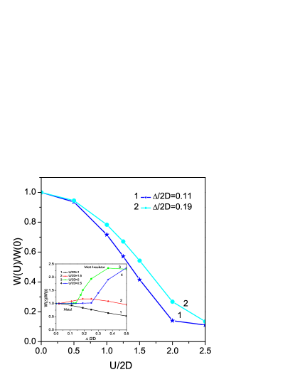
Figure 8: Dependence of the normalized optical integral of Anderson – Hubbard model on $U$ for different values of disorder $\Delta$. At the insert – similar dependence on $\Delta$ for different values of $U$. Curves 1,2 – “correlated metal”, transforming into Anderson insulator. Curves 3,4 – Mott insulator, obtained with the growth of $U$ from “correlated metal” or Anderson insulator.

IV.3 Localization length and phase diagram of 2D Anderson – Hubbard model.

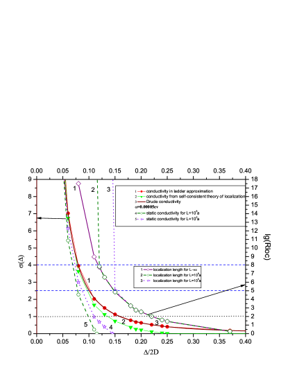
Figure 9: Left scale — dependence of conductivity on disorder $\Delta$ at fixed frequency $\omega=0.00005D$ and $U/2D=1$. Circles – ladder approximation, triangles – self-consistent theory of localization. Curve 3, practically coinciding with the results of ladder approximation, is obtained from Drude expression (22). Static conductivity for finite samples of sizes $L=10^{8}a$ (curve 4) and $L=10^{5}a$ (curve 5). Right scale — dependence of the logarithm of localization length on disorder $\Delta$: for infinite sample (curve 1) and for finite samples of sizes $L=10^{8}a$ (curve 2) and $L=10^{5}a$ (curve 3).

To proceed further on the left axis of Fig. 9 we present our data for the real part of conductivity at fixed and sufficiently small frequency $\omega=0.00005D$ plotted as a function of disorder strength $\Delta$. Circles show results of “ladder” approximation, triangles — results of self – consistent theory of localization (we take $U=0$ here). Curve 3, which practically coincides with results of the “ladder” approximation, is obtained from the usual Drude expression:

$$\sigma(\omega)=\sigma(0)\frac{\gamma^{2}}{\gamma^{2}+\omega^{2}},$$ (22)

where the static conductivity is given by $\sigma(0)=e^{2}N(0)D_{0}\approx\frac{e^{2}}{\hbar}\frac{\varepsilon_{F}}{2\pi\gamma}$, with $N(0)$ being the density of states at the Fermi level, $D_{0}$ is the classical diffusion coefficient, $\varepsilon_{F}\approx D$ is Fermi energy. Impurity scattering rate was taken as $\gamma=\pi N(0)\Delta^{2}\approx\frac{\pi}{2D}\Delta^{2}$. It can be seen that the noticeable contribution of localization corrections to conductivity (clear difference between curve 2 curves 1 and 3) appears only after conductivity drops below the values of the order of “minimal” metallic conductivity $\sigma_{0}=\frac{e^{2}}{\hbar}$ (our data for conductivity are actually normalized by this value in all figures). We shall see below that precisely in this region a kind of Anderson MIT (divergence of localization length) takes place in 2D systems of reasonable finite sizes.

On the right axis in Fig. 9 we show our data for the logarithm of localization length calculated from Eq. (18) as a function of disorder for infinite sample (curve 1) and for finite samples with $L=10^{8}a$ and $L=10^{5}a$ (curves 2 and 3). It is clearly seen that localization length grows exponentially as disorder drops but remains finite in infinite 2D sample, signifying the absence of Anderson transition. In finite samples localization length diverges at some critical disorder (depending on the system size) demonstrating the existence of an effective Anderson transition. From Fig. 9 it is seen that this critical disorder is achieved when localization length of an infinite system becomes comparable with characteristic size of the sample: $R_{loc}^{L\to\infty}\sim L$. It should be noted that in our approach, opposite to the results of Ref. Shapiro08, , localization length is practically independent of $U$, which leads to independence of critical disorder in 2D of correlation strength $U$. Similar result was obtained in our approach for 3D systems HubDis .

On the left axis of Fig. 9 disorder dependence of static conductivity for finite samples of the sizes $L=10^{8}a$ and $L=10^{5}a$ (curves 4 and 5) is shown. For finite systems with small disorder static conductivity is not zero (metal). It gradualy goes down while disorder grows and becomes zero at the same critical value where localization radius diverges on the approach from insulating phase in a finite sample. Static conductivity of finite samples in our calculations practicaly does not depend on correlation strength $U$. Rather significant difference between the values of static conductivity and that of conductivity at small but non zero frquencies seen in Fig. 9 comes from exponential smallness of frequency range of localization behavior mentioned above.

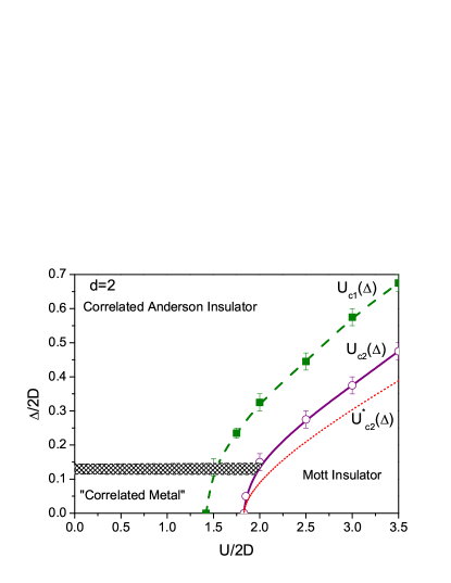
Figure 10: Phase diagram of two – dimensional paramagnetic Anderson – Hubbard model at zero temperature. The border of Mott insulator region $U_{c2}(\Delta)$ and the border of coexistence (hysteresis) region $U_{c1}(\Delta)$ are obtained from the evolution of the density of states, $U^{\ast}_{c2}(\Delta)$ is calculated from (24). Dashed stripe corresponds to the narrow region, where Anderson metal – insulator transition takes place in finite systems.

Let us now discuss our results for the phase diagram of 2D half – filled Anderson – Hubbard model, obtained from extensive DMFT+$\Sigma$ calculations of DOS and analysis of localization length behavior in finite 2D systems. The general form of this phase diagram in disorder – correlation ($\Delta,U$) plane is shown in Fig.10.

Dashed stripe in Fig. 10 corresponds to the region of an effective transition from Anderson insulator to “metallic” phase. It boundaries were determined by divergence of localization length in finite samples with characteristic sizes $L=10^{5}a$ (upper boundary) and $L=10^{8}a$ (lower boundary) (cf. Fig.9). It should be stressed that further increase of system size, e.g. 10 times up to $L=10^{9}a$, leads only to practically negligible downshift of the lower boundary (decrease of critical disorder) of dashed stripe in Fig. 10.

The dependence of $U_{c2}(\Delta)$, obtained from DOS behavior, determines the boundary for Mott transition and is defined by the disappearance of the quasiparticle peak in DOS and correlation gap opening at the Fermi level (cf. Fig.2,4).

In our previous work HubDis on 3D Anderson – Hubbard model we have proposed a simple explanation of $U_{c1,c2}(\Delta)$ dependence. Assuming that the controlling parameter of Mott – Hubbard transition given by the ratio of Hubbard interaction and effective bandwidth (depending on disorder) $\frac{U_{c1,c2}(\Delta)}{W_{eff}(\Delta)}$ is universal constant (independent of disorder), we get:

$$\frac{U_{c1,c2}(\Delta)}{W_{eff}(\Delta)}=\frac{U_{c1,c2}(0)}{W},$$ (23)

where $W_{eff}(\Delta)$ is an effective bandwidth in the presence of disorder, calculated at $U=0$ in self – consistent Born approximation (5). In 3D model HubDis the dependence of critical correlation strength on disorder $U_{c1,c2}(\Delta)$, obtained directly from the evolution of DOS, has shown quite satisfactory agreement with qualitative dependence obtained from Eq. (23)

In 2D model under consideration here, solution of Eq. (23) gives:

$$U^{\ast}_{c1,c2}(\Delta)=U_{c1,c2}(0)\frac{W_{eff}(\Delta)}{W}=$$

$$=U_{c1,c2}(0)\left(\frac{2{\Delta}^{2}}{W^{2}}ln\left(\frac{c+1}{c-1}\right)+c\right),$$ (24)

where $c=\sqrt{4\left(\frac{\Delta}{W}\right)^{2}+1}$. However, unlike in 3D case HubDis , $U_{c2}(\Delta)$ dependence, obtained from DOS evolution is clearly different from the qualitative one $U^{\ast}_{c2}(\Delta)$ (dotted line in Fig. 10), determined by Eq. (24). Probably, this is due to a significant change in the rectangular form of “bare”DOS with the growth of disorder $\Delta$, which is absent for semi – elliptic “bare” DOS used in 3D case in Ref. HubDis, .

As we already noted, with decrease of $U$ from insulating phase Mott transition occurs at $U=U_{c1}(\Delta)<U_{c2}(\Delta)$ and the coexistence (hysteresis) region is observed between $U_{c1}(\Delta)$ and $U_{c2}(\Delta)$ curves on phase diagramm Fig.10.

V Conclusion

We have used the generalized DMFT+$\Sigma$ approach to study basic properties of disordered and correlated Anderson – Hubbard model. Our method produces relatively simple interpolation scheme between two well studied limits — that of strongly correlated Hubbard model in the absence of disorder (DMFT and Mott – Hubbard MIT) and the case of 2D Anderson insulator in the infinite system without electron – electron interactions. It seems that the proposed interpolation scheme reflects all the qualitative features of Anderson – Hubbard model, such as behavior of the density of states and dynamic conductivity. The general structure of the phase diagram obtained in DMFT+$\Sigma$ approximation is also in reasonable agreement with the results of direct numerical simulations PB09 . At the same time, DMFT+$\Sigma$ approach is rather competitive in a sense of the amount of numerical work and allows direct calculations of all the basic observable characteristics of Anderson – Hubbard model.

It should be stressed that an effective Anderson transition obtained here in the case of finite size 2D systems is in no sense attributed to electronic correlations and follows directly from self – consistent theory of localization also in the absence of correlations.

The main shortcoming of the method used is the neglect of the interference between disorder scattering and Hubbard interaction, which leads to the independence of localization length and critical disorder $\Delta_{c}$ (in finite 2D systems) of correlation strength $U$. The importance of this kind of interference effects is known long ago Lee85 ; ma , though these can be taken into account only in the case of weak correlations and disorder. At the same time, the neglect of interference effects is the key point of our DMFT+$\Sigma$ approach, allowing to obtain rather simple and physically clear interpolation scheme, allowing to analyze the limits of strong correlations and disorder.

Another drastic simplification is our assumption of non magnetic (paramagnetic) nature of the ground state of Anderson – Hubbard model. The importance of magnetic (spin) effects in strongly correlated and disordered systems is obvious, as well as the importance of competition between different kinds of magnetic ground states georges96 .

Despite these shortcomings, our results seems rather attractive and reliable, e.g. with respect to strong disorder effects on Mott – Hubbard transition and the general form of the phase diagram at $T=0$. Our predictions for the general behavior of dynamic (optical) conductivity and disorder induced Mott insulator to effective “metal” transition can be directly compared with existing and future experiments.

VI Acknowledgements

We are grateful to Th. Pruschke for providing us with his effective NRG code.

This work is partly supported by RFBR grant 08-02-00021 and programs of fundamental research of the Presidium of RAS “Quantum physics of condensed state” and that of Physics Department of RAS “Strongly correlated electrons in solids”, as well as by the grant of the President of Russian Federation MK-614.2009.2 (IN).

References

- (1) P. A. Lee and T. V. Ramakrishnan, Rev. Mod. Phys. 57, 287 (1985); D. Belitz and T. R. Kirkpatrick. Rev. Mod. Phys. 66, 261 (1994).
- (2) E. Abrahams, P. W. Anderson, D. C. Licciardello, and T.V. Ramakrishnan. Phys. Rev. Lett. 42, 673 (1979).
- (3) B. L. Altshuler, A. G. Aronov and P. A. Lee. Phys. Rev. Lett. 44, 1288 (1980).
- (4) G. J. Dolan and D. D. Osheroff, Phys. Rev. Lett. 43, 721 (1979); D. J. Bishop, D. C. Tsui, and R. C. Dynes, Phys. Rev. Lett. 44, 1153 (1980); M. J. Uren, R. A. Davies, and M. Pepper. J. Phys. C 13, L985 (1980).
- (5) A. M. Finkelshtein. Sov. Phys. JETP 75, 97 (1983); C. Castellani et al.. Phys. Rev. B 30, 527 (1984).
- (6) S. V. Kravchenko and M. P. Sarachik. Rep. Prog. Phys. 67, 1 (2004).
- (7) E. Abrahams, S. V. Kravchenko and M. P. Sarachik. Rev. Mod. Phys. 73, 251 (2001)
- (8) N. F. Mott. Proc. Phys. Soc. A 62, 416 (1949); Metal–Insulator Transitions, 2nd edn. (Taylor and Francis, London 1990).
- (9) P. W. Anderson. Phys. Rev. 109, 1492 (1958).
- (10) V. Dobrosavljević and G. Kotliar. Phys. Rev. Lett. 78, 3943 (1997).
- (11) V. Dobrosavljević, A. A. Pastor, and B. K. Nikolić. Europhys. Lett. 62, 76 (2003).
- (12) K. Byczuk, W. Hofstetter, D. Vollhardt. Phys. Rev. Lett. 94, 056404 (2005)
- (13) E.Z. Kuchinskii, I.A. Nekrasov, M.V. Sadovskii, Zh. Eksp. Teor. Fiz. 133, 670 (2008).
- (14) P. Henseler, J. Kroha, and B. Shapiro, Phys. Rev. B 77, 075101 (2008).
- (15) P. Henseler, J. Kroha, B. Shapiro, Phys. Rev. B 78, 235116 (2008)
- (16) M.E. Pezzoli, F. Becca, arXiv: 0906.4870
- (17) W. Metzner and D. Vollhardt. Phys. Rev. Lett. 62, 324 (1989).
- (18) D. Vollhardt, in Correlated Electron Systems, edited by V. J. Emery, World Scientific, Singapore, 1993, p. 57.
- (19) Th. Pruschke, M. Jarrell, and J. K. Freericks. Adv. Phys. 44, 187 (1995).
- (20) A. Georges, G. Kotliar, W. Krauth, and M. J. Rozenberg. Rev. Mod. Phys. 68, 13 (1996).
- (21) M. Ulmke, V. Janiš, and D. Vollhardt. Phys. Rev. B 51, 10411 (1995).
- (22) R. Vlaming and D. Vollhardt. Phys. Rev. B 45, 4637 (1992).
- (23) E.Z.Kuchinskii, I.A.Nekrasov, M.V.Sadovskii. Pis’ma Zh. Eksp. Teor. Fiz. 82, 217 (2005) [JETP Lett. 82, 198 (2005)].
- (24) M.V. Sadovskii, I.A. Nekrasov, E.Z. Kuchinskii, Th. Prushke, V.I. Anisimov. Phys. Rev. B 72, 155105 (2005).
- (25) E.Z. Kuchinskii, I.A. Nekrasov, M.V. Sadovskii. Fizika Nizkikh Temperatur 32, 528 (2006) [Low Temp. Phys. 32, 398 (2006)].
- (26) E.Z. Kuchinskii, I.A. Nekrasov, M.V. Sadovskii. Phys. Rev. B 75, 115102 (2007).
- (27) K.G. Wilson, Rev. Mod. Phys. 47, 773 (1975); H.R. Krishna-murthy, J.W. Wilkins, and K.G. Wilson, Phys. Rev. B 21, 1003 (1980); ibid. 21, 1044 (1980); A.C. Hewson, The Kondo Problem to Heavy Fermions. Cambridge University Press, 1993.
- (28) R. Bulla, A.C. Hewson and Th. Pruschke, J. Phys. – Condens. Matter 10, 8365(1998).
- (29) R. Bulla, Phys. Rev. Lett. 83, 136 (1999); R. Bulla, T.A. Costi and D. Vollhardt. Phys. Rev. B 64, 045103 (2001).
- (30) D. Vollhardt and P. Wölfle, Phys. Rev. B 22, 4666 (1980); Phys. Rev. Lett. 48, 699 (1982)
- (31) P. Wölfle and D. Vollhardt, in Anderson Localization, eds. Y. Nagaoka and H. Fukuyama, Springer Series in Solid State Sciences, vol. 39, p.26. Springer Verlag, Berlin 1982.
- (32) A.V. Myasnikov, M.V. Sadovskii, Fiz. Tverd. Tela 24, 3569 (1982) [Sov. Phys.-Solid State 24, 2033 (1982) ]; E.A. Kotov, M.V. Sadovskii. Zs. Phys. B 51, 17 (1983).
- (33) M.V. Sadovskii, in Soviet Scientific Reviews – Physics Reviews, ed. I.M. Khalatnikov, vol. 7, p.1. Harwood Academic Publ., NY 1986.
- (34) D. Vollhardt, P. Wölfle, in Electronic Phase Transitions, eds. W. Hanke and Yu.V. Kopaev, vol. 32, p. 1. North–Holland, Amsterdam 1992.
- (35) M.V. Sadovskii. Diagrammatics. World Scientific, Singapore 2006.
- (36) E.Z. Kuchinskii, N.A. Kuleeva, M.V. Sadovskii, I.A. Nekrasov. Zh. Eksp. Teor. Fiz. 107, 281 (2008) [JETP 107, 281 (2008)]
- (37) R. Kubo. J. Phys. Soc. Japan 12, 570 (1957).