Bouncing transient currents and SQUID-like voltage in nano devices at half filling

Abstract

Nanorings asymmetrically connected to wires show different kinds of quantum interference phenomena under sudden excitations and in steady current conditions. Here we contrast the transient current caused by an abrupt bias to the magnetic effects at constant current. A repulsive impurity can cause charge build-up in one of the arms and reverse current spikes. Moreover, it can cause transitions from laminar current flow to vortices, and also change the chirality of the vortex. The magnetic behavior of these devices is also very peculiar. Those nano-circuits which consist of an odd number of atoms behave in a fundamentally different manner compared to those which consist of an even number of atoms. The circuits having an odd number of sites connected to long enough symmetric wires are diamagnetic; they display half-fluxon periodicity induced by many-body symmetry even in the absence of electron-phonon and electron-electron interactions. In principle one can operate a new kind of quantum interference device without superconductors. Since there is no gap and no critical temperature, one predicts qualitatively the same behavior at and above room temperature, although with a reduced current. The circuits with even site numbers, on the other hand, are paramagnetic.

I Introduction

The last decade has witnessed a growing interest in the persistent currents in quantum rings threaded by a magnetic flux $\phi.$ This problem has many variants. The rings of interest may contain impurities, may interact with quantum dots or reservoirs. Moreover, both continuous and discrete formulations have been used to date, with similar results. Aligiaaligia modeled the persistent currents in a ring with an embedded quantum dot. Theoretical approaches to one-dimensional and quasi-one-dimensional quantum rings with a few electrons are reviewed by S.Viefers and coworkersviefers ; see also the recent review by S. Maitimaiti where it is pointed out that central issues like the diamagnetic or the paramagnetic sign of the low-field currents of isolated rings are still unsettled. The present paper, instead, is devoted to rings connected to circuits. It is clear that the connection to wires substantially modifies the problem, but here we point out that some of the modifications are not obvious and lead to quite interesting and novel consequences.

Simple quantum rings can be connected to biased wires in such a way that the current flows through inequivalent paths. In the present, exploratory paper, we consider a tight-binding ring with $N$ sites attached to two one-dimensional leads and specialize on the half-filled system. We show that this innocent-looking situation produces peculiar phenomena like bouncing transients i.e. current spikes in the reverse direction, and a new sort of simulated pairing. These systems could find applications in spintronic or fast electronic devices exploiting spikes in the onset currents, or also in steady current conditions when used to measure local magnetic fields. Thus, our motivation is twofold. On one hand, we look for the conditions that can produce novel phenomena in the transient current when the system is biased. On the other hand we are interested in the bias that develops across the system in steady current conditions when it is used like a SQUID. After presenting the model in the next Section, in Section III we present the formalism and in Section IV apply it to situations where transient currents through the circuit are large and appear to bounce to a direction contrary to the main stream. We then discuss the currents inside the device, with vortices that can be clockwise or counterclockwise depending on the parameters. The nontrivial topology allows interference effects of the Aharonov-Bohm type in one-body experiments, but in addition here, a many-body symmetry comes into play when the ring has an odd number of atoms. The interplay of symmetry and topology may lead to a diamagnetic behavior with a half-fluxon periodicity which looks like a typical superconducting pattern as shown in Section V. The possible operation of the circuit as a magnetometer is also suggested. Our main results are summarized in the concluding Section VI.

II Model

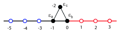
Figure 1: Sketch of the site numbering and site energies of the triangular ring, shown with part of the leads. The impurity is denoted by its energy $\epsilon_{c}$ while we shall set $\epsilon_{a}=\epsilon_{b}=0.$ The hopping integrals in the absence of magnetic field are $t_{ab}=t_{bc}=t_{ca}=t_{dev}$.

The Hamiltonian describing the left ($L$) and right ($R$) one-dimensional leads is

$$H_{\alpha}=t_{h}\sum_{m=0}^{\infty}(c^{{\dagger}}_{m,\alpha}c_{m+1,\alpha}+{\rm h.c.}),$$ (1)

where $t_{h}$ is the hopping integral between nearest neighbor sites and $c_{m+1,\alpha}$ annihilates an electron at site $m+1$ in wire $\alpha=L,R$. The spin indices are not shown in order to simplify the notation. The energy window of both $L$ and $R$ continua is $(-2|t_{h}|,2|t_{h}|)$ and the half-filled system corresponds to having a chemical potential $\mu=0$. In this work we consider $N$-sided polygonal devices described by the Hamiltonian

$$H_{\rm ring}=\sum_{<m,n>=1}^{N}(t_{mn}d^{{\dagger}}_{m}d_{n}+{\rm h.c.})$$ (2)

where $d_{n}$ are Fermion annihilation operators inside the device and $t_{mn}$ is the hopping between site $m$ and site $n$. In the rest of the paper we specialize to the case $t_{mn}=0$ if $m$ and $n$ are not nearest neighbors and $t_{mn}\equiv t_{dev}e^{i\alpha(m,n)}$, where $e^{i\alpha(m,n)}$ is a phase factor, otherwise. The simplest example is the triangular model ($N=3$) shown in Figure 1. In this case we also label the sites with letters and consider a non-magnetic impurity at the vertex site $c$ of strength $\epsilon_{c}$:

$$H_{\rm ring}=\sum_{<m,n>\in\{a,b,c\}}(t_{mn}d^{{\dagger}}_{m}d_{n}+{\rm h.c.})+\epsilon_{c}n_{c},$$ (3)

with $n_{c}=d^{{\dagger}}_{c}d_{c}$.

The wires will be attached at a couple of sites in the ring that will be specified case by case below by using a tunneling Hamiltonian $H_{T}$ with hopping parameter $t_{h}$. Thus, the equilibrium Hamiltonian reads

$$H_{0}=H_{L}+H_{R}+H_{\rm ring}+H_{T}$$ (4)

while for times $t>0$

$$H(t)=H_{0}+H_{\rm bias}(t),$$ (5)

where

$$H_{\rm bias}(t)=\sum_{\alpha=L,R}\sum_{m=0}^{\infty}V_{\alpha}(t)n_{m,\alpha},$$ (6)

with $n_{m\alpha}=c^{{\dagger}}_{m\alpha}c_{m\alpha}$. The bias shifts the energy of the $\alpha$ sites by a constant amount, with a time dependence $V_{\alpha}(t)$.

The electron number current operator between sites $m$ and $n$ connected by a bond with hopping integral $\tau_{mn}$ ($\tau_{mn}=t_{h}$ or $t_{dev}e^{i\alpha(m,n)}$ inside the device) is determinedcaroli by imposing the continuity equation

$$J_{mn}=-\frac{i}{\hbar}\tau_{mn}c^{{\dagger}}_{n}c_{m}+{\rm h.c.}.$$ (7)

For ring sites, $c$ operators will be replaced by $d$ ones.

III Formalism

In the partition-free approachcini80 the formula for the time-dependent averaged current through the $m-n$ bond reads

$$\langle J_{mn}(t)\rangle={\rm Tr}\left[\hat{f}^{(0)}U^{{\dagger}}(t)J_{mn}U(t)\right],$$ (8)

with

$$\hat{f}^{(0)}=\frac{1}{e^{\beta(H_{0}-\mu)}+1},$$ (9)

the Fermi function computed at the equilibrium Hamiltonian $H_{0}$ and $U(t)$ the evolution operator. In the actual calculations we have adopted a local view and write the electron number current

$$\langle J_{mn}(t)\rangle=$$

$$\frac{2e}{\hbar}{\rm Im}\left[\tau_{mn}\sum_{rs}\langle n|U^{\dagger}(t)|r\rangle\langle s|U(t)|m\rangle f(r,s)\right],$$ (10)

where $f(r,s)=\langle r|\hat{f}^{(0)}|s\rangle$ is the matrix element of $\hat{f}^{(0)}$ between one-particles states localized at sites $r$ and $s$. In this way we observed that far sites in the wires come into play one after another with a clear-cut delay. One can simulate infinite leads with wires consisting of $l$ sites and obtain quite accurate currents for times up to $t=\frac{\hbar}{t_{h}}{l\over 3};$ the absence of more distant sites does not change the results in any appreciable measure. Eventually, when $t$ is increased at fixed length $l$, the information that the wires are finite arrives quite suddenly and a fast drop of the current takes place.psc.2008

Another useful expression for the bond-current which holds for step-function switching of the bias can be obtained by inserting into Equation (III) complete sets $\psi_{1},\psi_{2}$ of $H$ eigenstates (in the presence of the bias) with energy eigenvalues $E(\psi_{1}),E(\psi_{2})$; one gets

$$\langle J_{mn}(t)\rangle=-\frac{2e}{\hbar}Im\left(t_{mn}\sum_{\psi_{1},\psi_{2}}e^{i\frac{(E(\psi_{1})-E(\psi_{2})t}{\hbar}}\right.$$

$$\left.\langle n|\psi_{1}\rangle\langle\psi_{2}|m\rangle\sum_{n_{1},n_{2}}\langle\psi_{1}|n_{1}\rangle\langle n_{2}|\psi_{2}\rangle f(n_{1},n_{2})\right).$$ (11)

This informs us about the frequency spectrum of the current response. The frequencies arise from energy differences between the eigenstates of the Hamiltonian of the full circuit with the bias included. The weights at a given bond depend in a simple way on the eigenfunctions at the bond and on the equilibrium occupation of single-electron states. If there are sharp discrete states outside the continuum, $\langle J_{mn}(t)\rangle$ has an oscillatory component, otherwise it tendscini80 to the current-voltage characteristics asymptotically as $t\rightarrow\infty$.

IV Switch-on currents

We study the triangular model of Figure 1 with $t_{ab}=t_{bc}=t_{ca}=t_{dev}$ and $t_{dev}=t_{h}$ for the sake of definiteness. Our main idea in the model calculations has been to study the $\epsilon_{c}$ dependence of the transient in order to look for marked out-of-equilibrium behavior, like vortex formation, or large charge build-up followed by strong current spikes. Also, one is interested in conditions that produce a fast change of the response with $\epsilon_{c},$ since possibly in such situations magnetic impurities can produce strong spin polarization.

Below we present numerical results for 150 sites in the leads (which guarantee an accurate propagation up to times $20\hbar/t_{h}$) and switch on a constant bias $V_{L}=V=0.5$ and $V_{R}=0$ at $t=0$. In the steady state it tends to produce a negative local current flow (in the sense that the electron number current goes from the right to the left wire).

IV.1 Total current

In Figure 2 we show the time-dependence of the number current in $\frac{t_{h}}{\hbar}$ units on the bond between sites -3 and -4 for different values of $\epsilon_{c}.$

IV.1.1 Long-time limit

The times we are considering are short enough to enable us to use the finite-lead scheme specified above, however the system already clearly approaches the steady state for all $\epsilon_{c}$. The effect of the impurity at site $c$ on the asymptotic current is much stronger than one could have expected from any classical analogue. The current at $\epsilon_{c}=-1$ (in units of $t_{h}$) is more than an order of magnitude larger than it is at $\epsilon_{c}=+1.$ Moreover, in a range around $\epsilon_{c}=0$ the negative current increases (that is, its absolute value decreases) with increasing $\epsilon_{c},$ as one could expect if the repulsive site were an obstruction to the current flow. However this view is not in line with the fact that a further increase of $\epsilon_{c}$ increases the conductivity of the device. The correct interpretation is that the conductivity is ruled by quantum interference between the $a-b$ and $a-c-b$ paths, particularly by electrons around the Fermi-level.

IV.1.2 Short and intermediate times

Here we are in position to see how this quantum interference develops in time. It takes a time $\sim\frac{\hbar}{t_{h}}$ for the current to go from zero to the final order-of-magnitude; then for some $\frac{\hbar}{t_{h}}$ large oscillations occur, which appear to be damped with a characteristic time $\sim 10\frac{\hbar}{t_{h}}.$ The oscillations have characteristic frequencies that in accordance with Equation (III) increase by increasing the hopping matrix elements or modifying the device in any way that enhances the energy level differences. It can be seen that the damping of the oscillations is not exponential, and characteristic times of the order of 10 $\frac{t_{h}}{\hbar}$ are also noticeable.

Figure 2 shows that at $\epsilon_{c}=0$ the current quickly approaches $-0.08\frac{t_{h}}{\hbar}$, but at short times the spread of values of the currents is larger than it is at asymptotic times. A negative impurity like $\epsilon_{c}=-1$ produces a spike whose magnitude exceeds by $\sim 30$ per cent the steady state value $\sim-0.12\frac{t_{h}}{\hbar}$, while a positive $\epsilon_{c}$ reduces the conductivity of the device. The dependence of the current on $\epsilon_{c}$ and time is involved, with the $\epsilon_{c}=1$ case which does not belong to the region delimited by $\epsilon_{c}=0$ and $\epsilon_{c}=2$ curves. The $\epsilon_{c}=0.8$ and $\epsilon_{c}=1.0$ curves that produce small negative currents at long times are most interesting. They even go positive for some time interval $\sim\frac{\hbar}{t_{h}}$. Positive currents go backwards. This bouncing current is a quantum interference effect, which takes the system temporarily but dramatically out of equilibrium and in counter-trend to the steady state. The main spike of reversed current is much larger than the long-time direct current response. Next, to understand what produces the bouncing current, we look at the transport inside the triangular device.

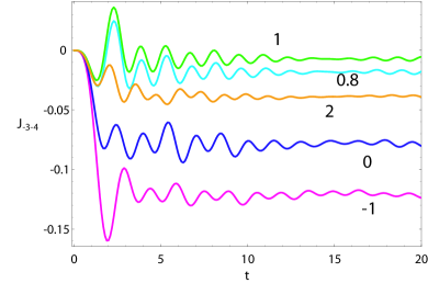
Figure 2: Time-dependence of the current on the bond between the sites -3 and -4. The numbers shown close to each curve indicate the values of $\epsilon_{c}$. From bottom $\epsilon_{c}=-1,0,2,08,1$ in units of $t_{h}$. Here and below $t$ is in $\frac{\hbar}{t_{h}}$ units and the current is in units of $\frac{t_{h}}{\hbar}$.

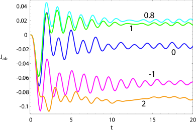
Figure 3: Time-dependence of $\langle J_{ab}\rangle$. The numbers shown close to each curve indicate the values of $\epsilon_{c}$. From bottom, $\epsilon_{c}=2,-1,0,1,0.8$ in units of $t_{h}$.

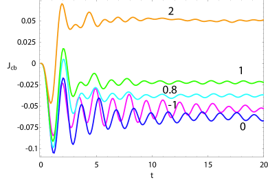
Figure 4: Time-dependence of $\langle J_{cb}\rangle$. The numbers shown close to each curve indicate the values of $\epsilon_{c}$. From bottom, $\epsilon_{c}=0,-1,0.8,1,2$ in units of $t_{h}$.

IV.2 Laminar flow and Vortices

In Figures 3 and 4 we report the time-dependent $\langle J_{ab}\rangle$ and $\langle J_{bc}\rangle$ at times $0<t<\frac{20\hbar}{t_{h}}$ for $\epsilon_{a}=\epsilon_{b}=0$ and various values of $\epsilon_{c}$. When the site $c$ is attractive for electrons (that is, $\epsilon_{c}<0$), despite some transient oscillations, the current remains negative, both on the $a$-$b$ and $c$-$b$ bonds; the current flows from $b$ towards $a$ and $c$, so the flow is laminar. The magnitude of the current on the $a$-$b$ and $c$-$b$ bonds is comparable. Although site $c$ may have a high electron population, the local current does not concentrate on either bond.

For $\epsilon_{c}=0.8$ and $\epsilon_{c}=1.0$ the current $J_{ab}$ on the $a$-$b$ bond (Figure 3), after a negative transient spike, produces a positive one, which is the main contribution to the bouncing current noted above. This behavior can be understood in terms of a strong charge build-up on the $a$-$c$-$b$ arm of the ring during the first burst following the switching of the bias, which eventually triggers the temporary back-flow. After the burst, $J_{ab}$ remains positive ($\epsilon_{c}=0.8$ and $\epsilon_{c}=1.0$ curves in Figure 3) while $J_{cb}$ remains negative value ($\epsilon_{c}=0.8$ and $\epsilon_{c}=1.0$ curves in Figure 4). In other terms, we observe the formation of an anti-clock-wise current vortex.

Remarkably and unexpectedly, by increasing $\epsilon_{c}$ one reaches a critical value beyond which the vortex becomes clock-wise, as one can see from the $\epsilon_{c}=2$ curves in Figures 3 and 4. This conclusion is unavoidable since the current changes sign in both arms of the circuit. The total current (Figure 2) remains negative, as one expects. We were unable to find any simple qualitative explanation for the inversion of the vortex. In general the critical value of $\epsilon_{c}$ depends on the bias $V$ and for $V=0.5$ is about 1. Moreover, we emphasize that the current across a strongly repulsive site with $\epsilon_{c}=2$ is still comparable in magnitude with the one on the $a$-$b$ bond.

V Many-body symmetry and Magnetic Response

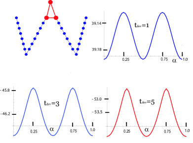
Figure 5: The ${\phi\over 2}$ periodicity arising from the symmetry-induced false pairing. Top left: the triangular device connected to $\Lambda=$14-site wires. The other panels show the ground state energy $E_{0}(\alpha)$ versus $\alpha.$ Top right: $t_{dev}=t_{h}$. Bottom left: $t_{dev}=3t_{h}$. Bottom right: $t_{dev}=5t_{h}$.

Nanoring devices asymmetrically connected to wires of $\Lambda$ sites each are even more peculiar for their magnetic properties. Here we restrict to the case $\epsilon_{c}=0$. The magnetic flux $\phi$ through the ring is inserted by the Peierls prescriptiontopics ,canright

$$t_{ac}\rightarrow t_{ac}e^{2\pi i\alpha},$$ (12)

where $\alpha=\frac{\phi}{\phi_{0}}$ and $\phi_{0}=\frac{hc}{e}$ is the magnetic flux quantum. In the case of vanishing bias, in stationary conditions one finds a diamagnetic current which is confined to the triangular ring. In Figure 5 we illustrate our results. We sketch a triangular device connected to 14-site leads and the ground state energy $E_{0}(\alpha)$ versus $\alpha=\frac{\phi}{\phi_{0}}$ for $t_{dev}\equiv t_{ab}=t_{bc}=t_{ca}=1,3$ and 5. The expected periodicity in $\alpha$ with period 1 due to gauge invariance is of course observed. Strikingly, however, we notice that the period is actually ${1\over 2}$, and the system is diamagnetic, i.e. the energy increases when the un-magnetized system is put in a magnetic field. In other terms, $E_{0}(\alpha)$ looks like the ground state energy of a superconducting ring, although this is a non-interacting model and the spectrum is gapless.

One could wander how the positive diamagnetic response at small fields arises, since the initial dependence of the total energy on the flux is quadratic and the second-order correction is always negative. However this is an apparent paradox. The energy change is due to a perturbation $t_{dev}(e^{2\pi i\alpha}-1)\sim t_{dev}(2\pi i\alpha-2\pi^{2}\alpha^{2})$ which is the effect of changing the phase of one bond. First order perturbation theory corresponds to compute the current operator over the ground state and it is zero. The quadratic contribution is given by second-order perturbation theory in $2\pi i\alpha t_{dev}$ plus a term coming from the first-order correction in $-2\pi^{2}\alpha^{2}t_{dev}$. The former term is always negative while the second term can be either positive or negative.

V.1 Nontrivial role of the wires

The results in Figure 5 are striking because the isolated nano-ring with 3 sites at half filling does not simulate any superconducting behavior; instead, it yields a paramagnetic pattern, symmetric around $\alpha=\frac{1}{2}$ ($\alpha=1$ is equivalent to $\alpha=0$). One can easily work out the lowest energy eigenvalue $E_{0}$ with 3 electrons. $E_{0}=-3$ for $\alpha=0$ sinks to $E_{0}=-2\sqrt{3}\sim-3.46$ at $\alpha={1\over 4},$ and raises again to $E_{0}=-3$ at $\alpha={1\over 2}.$ Thus, there is a half-fluxon periodicity at half filling, but $\alpha=0$ and $\alpha={1\over 2}$ are maxima and correspond to degenerate 3-body states.

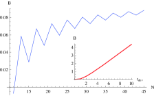
Figure 6: Dependence of the barrier hight $B$ on the total number N of sites, which include the triangular device and the $L$ and $R$ leads. The parameters are the same as in Fig. 6. The line is a guide for the eye. Note that for short leads $B$ is negative. The inset shows the almost linear dependence of $B$ on $t_{dev}=t_{ab}=t_{ac}=t_{bc}$.

The superconductor-like response requires the presence of wires, despite the fact that the diamagnetic currents induced by the field are strictly confined to the triangular device. The currents do not visit the wires, but the electron wave functions do. In order to produce the double minimum, the wires must be rather long. The barrier height $B=E_{0}(\frac{1}{4})-E_{0}(0)$ depends on the total number of atoms ${\cal N}=3+2\Lambda$ (see Figure 6) and below a minimum length $B<0$. In Fig. 8 we plot the dependence of the barrier $B$ on the number of sites ${\cal N}=3+2\Lambda$ of the leads. We observe that $B$ saturates with increasing ${\cal N}$. This finding is noteworthy and unusual. The inset of Figure 6 shows how $B$ depends on $|t_{dev}|$ and suggests that except for an initial quadratic region the dependence is basically linear. With hopping integrals in the eV range $B$ easily exceeds room temperature.

V.2 Bipartite and not bipartite wired devices

Next we investigate why the effect takes place in this geometry and at half filling. A crucial observation is that the system depicted in Figure 5 is not a bipartite graph. By contrast, Figure 7 shows the flux dependence of the ground state of a bipartite graph, namely, a square device connected to wires. The response is paramagnetic since the ground state at $\phi=0$ is degenerate, the field lifts the degeneracy, a Zeeman effect occurs, and the ground state energy is lowered. In addition, the trivial periodicity is observed.

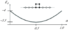
Figure 7: Flux-dependent energy $E_{0}(\alpha)$ for a square device with $t_{dev}=t_{h}$. Notice the scale, the paramagnetic behavior, and the level crossing at no flux. The central part of the system, with the device and the beginning of the wires, is also shown.

In Figure 8 we add one site to the device, and the diamagnetic double minimum pattern is found for the resulting pentagonal device, which does not produce a bipartite graph. Based on this observation and on a symmetry analysis, we can show that the half-fluxon periodicity ($E_{0}(\frac{1}{2})=E_{0}(0)$) holds. This is a theorem which holds for any ring with an odd number of atoms connected to leads of any length provided that the site energies vanish.

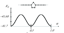
Figure 8: Flux-dependent energy $E_{0}(\alpha)$ for a pentagonal device with $t_{dev}=t_{h}$. Notice the diamagnetic behavior, and the absence of level crossing at no flux. The central part of the system, with the device and the beginning of the wires, is also shown.

V.3 Symmetry analysis

Let $C$ denote the charge conjugation operation (or electron-hole canonical transformation) $c_{\alpha}\rightarrow b_{\alpha}^{\dagger}$, where $c_{\alpha}$ annihilates electrons and $b^{\dagger}_{\alpha}$ creates a hole with quantum numbers $\alpha$. $C$ is equivalent to $\tau_{mn}\rightarrow-\tau_{mn}$ throughout, or, since the site energies vanish, to $H\rightarrow-H$.

We recall two elementary results of graph theory: 1) an isolated ring is a bipartite graph if and only if it has an even number of atoms 2) adding wires of any length does not change the result.

In bipartite lattices, $C$ is equivalent to a sign change of alternating orbitals, which is a gauge transformation. Hence, $H$ and $-H$ have the same one-body spectrum, that is, the spectrum is top-down symmetric.

For the wired triangular ring and any other non-bipartite graph, the one-body spectrum is not top-down symmetric (exceptexcept at $\alpha=\frac{1}{4},\alpha=\frac{3}{4}$) so it does not appear the same after the transformation, and $C:H\rightarrow-H$ is equivalent to changing the sign of one bond in the ring. But this is just the effect of the operation $F:\alpha\rightarrow\alpha+\frac{1}{2}$ which inserts half a fluxon in the ring. Therefore the combined operation $C\circ F$ is an exact symmetry of the many-electron state which holds at half filling. It is clear that $F:H\rightarrow-H$ i.e. $F$ turns the spectrum upside-down.

However, as noted above, the spectrum is not top-down symmetric and when at $\phi={\phi_{0}\over 2}$ the occupied and empty spin-orbitals have exchanged places the system does not quite look like it was at $\alpha=0.$ For instance, at the top of the spectrum of the device of Figure 5 at $\alpha=0$ there is an empty split-off state. At $\alpha=0.5$ this becomes a deep state below the band. Nevertheless, we wish to prove that the many-body ground state energy $E_{0}(\alpha)$ at $\alpha={1\over 2}$ is exactly the same as at $\alpha=0.$

The reason lies in another symmetry of the many-body state at half filling. In terms of one-body spin-orbital levels, Tr$H(\alpha)=0$ implies

$$E_{0}(\alpha)=\sum_{i}n_{i}(\alpha)\epsilon_{i}(\alpha)=-\sum_{i}(1-n_{i}(\alpha))\epsilon_{i}(\alpha).$$ (13)

Since under $F$ the negative of the energy of the unoccupied levels coincide with the energy of the occupied ones, we have $\epsilon_{i}(\frac{1}{2})=-\epsilon_{i}(0)$ and $(1-n_{i}(\frac{1}{2}))=n_{i}(0)$ from which it follows that

$$E_{0}(\frac{1}{2})=-\sum_{i}(1-n_{i})\epsilon_{i}(\frac{1}{2})=E_{0}(0).$$ (14)

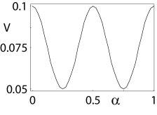
Figure 9: Operation of the triangular device with $\epsilon_{a}=\epsilon_{b}=\epsilon_{c}=0$ and $t_{dev}=t_{h}$ used a a SQUID thread by a flux $\phi$. A fixed current $J=0.016\frac{t_{h}}{\hbar}$ flows through the device. The right wire site energies are raised by $V_{R}=V(\phi)$, the left wire site energies are lowered by $V_{L}=-V(\phi)$, and $V$ is adjusted in order to keep $J$ fixed. The $V(\phi)$ versus $\phi$ plot is perfectly periodic with a half-fluxon period and simulates a superconducting SQUID, although no superconductors are needed.

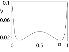
Figure 10: Here we present the same thought experiment as in the previous Figure, except that the device is a square with $t_{dev}=t_{h}$ threaded by a flux $\phi$ with zero on-site energies. The SQUID-like behavior and the half-fluxon periodicity are lost, as expected in bipartite graphs (see text). In this particular example the lower-left bond was raised to $1.2t_{h}$ in order to study the effects of a slight deformation of the square, but no relevant departure from the perfect square behavior was found.

V.4 Superconductor-free Quantum Interference Device

The superconducting quantum interference device (SQUID) consists of two superconductors separated by thin insulating layers to form two parallel Josephson junctions, and can be used as a magnetometer to detect tiny magnetic fields. If a constant biasing current is maintained in the SQUID device, the measured voltage oscillates with the change in the magnetic flux, and by counting the oscillations one can evaluate the flux change which has occurred. In principle one can produce Josephson-like oscillations without the need of superconductivity; if the device can be realized this can be a physical principle of interest for applications, maybe even at room temperature. Impurities and any disturbance affecting the quantum coherence can lower the operating temperature, but since in principle $B$ can be as large as 1eV we believe there is enough motivation for an experimental activity on this idea. According to the above arguments, the triangular pentagonal and other odd-numbered polygonal devices should simulate a SQUID, while bipartite graphs should present a normal behavior. We have performed the thought experiment with the triangular device connected to infinite wires; the results are reported in Figure 9. We keep a fixed current $J$ flowing through the device by adjusting $V(\phi)$, while the flux $\phi$ threading the device is varied. It can be seen that the plot of $V(\phi)$ versus $\phi$ is periodic with a half-fluxon period. The system simulates a SQUID, although no superconductors are needed. A counter-example is given in Figure 10, where the triangular device is replaced by a square one and the effect disappears.

VI Conclusions

We have shown that simple asymmetric closed circuits have rather subtle properties when unsymmetrically connected to the biased circuit, that could also be useful for designing new kinds of devices. We have found that an impurity site of energy $\varepsilon_{c}$ in the longer arm of a triangular device can cause a transient bouncing current, which goes in the opposite direction than the long-time current and is much more intense but lasts for a short time. Looking at the current distribution inside the device, $\varepsilon_{c}<0$ favors a laminar current flow; instead, $\varepsilon_{c}>0$ produces an anticlockwise current vortex; when a critical value is exceeded, however, the vortex chirality reverses. Further, we have shown that a class of closed circuits at half filling have a degenerate ground state which is paramagnetic, i.e. gains energy in a magnetic field by a Zeeman splitting. The magnetic behavior is completely changed when the circuits are connected to leads and form a non-bipartite lattice. Long leads constitute an essential requirement and although the diamagnetic currents are confined to the ring, the leads modify the magnetic properties substantially. With long enough wires one obtains a diamagnetic behavior with half fluxon periodicity and a robust barrier separating the energy minima at 0 and ${\phi_{0}\over 2}$. This pattern mimics a superconducting ring although there are no gap, no interactions, no critical temperature. We have traced back the origin of this fake superconducting behavior to a combination of charge-conjugation and flux which provides a symmetry of the many-electron determinantal state. Finally we have shown that in principle one can extend this simulation to the point of building a functioning interference device capable of measuring local fields and analogous to a SQUID but working even above room temperature. It cannot be excluded that even-sided circuits can be useful for the same purpose, and indeed Figure 10 suggests that one could do so, exploiting the trivial periodicity. The signal in Figure 9, however, is much more monochromatic, and this suggests that the odd-sided version should make it much easier to read-off the magnetic field intensity from the amplitude of the voltage oscillation.

References

- (1) A. A. Aligia, Phys. Rev. B66,165303 (2002)
- (2) S. Viefers, P. Koskinen, P. Singha Deo and M. Manninen,Physica E: Low-dimensional Systems and Nanostructures 21, 1 (2004), Pages 1-35
- (3) Santanu Maiti, cond-mat.mes-hall 0812.0439
- (4) C. Caroli, R. Combescot, P. Nozieres and D. Saint James, J. Phys. C 4, 916 (1971).
- (5) M. Cini, Phys. Rev. B 22 5887 (1980)
- (6) E. Perfetto, G. Stefanucci and M. Cini, Phys. Rev. B 78, 155301 (2008).
- (7) see for instance Michele Cini,”Topics and Methods in Condensed Matter Theory”, Springer Verlag (2007)
- (8) G.S. Canright and S.M. Girvin, Int. J. Mod. Phys. B 3, 1943 (1989)
- (9) G. Stefanucci, E. Perfetto, S. Bellucci and M. Cini, Phys. Rev B 79, 073406 (2009).
- (10) A. Callegari, M. Cini , E. Perfetto, and G. Stefanucci, Eur. Phys. J. B 34, 455 466 (2003)
- (11) M. Ernzerhof, H. Bahmann, F. Goyer, M. Zhuang and P. Rocheleau, J. Chem. Th. Comput. 2, 1291 (2006).
- (12) As noted above, the one-body spectrum is not generally top-down symmetric; at , out of the eigenvalues, are negative and positive; at , because of the turnover of the spectrum, are positive and L+1 negative. At , by a gauge transformation on one can change the signs of all real bonds, then by complex conjugation one obtains ; since and must have the same (real) eigenvalues, it follows that one eigenvalue vanishes and the spectrum is top-bottom symmetric like in bipartite lattices.