Spectral filtering in quantum Y-junction

Abstract

We examine scattering properties of singular vertex of degree $n=2$ and $n=3$, taking advantage of a new form of representing the vertex boundary condition, which has been devised to approximate a singular vertex with finite potentials. We show that proper identification of $\delta$ and $\delta^{\prime}$ components in the connection condition between outgoing lines enables the designing of quantum spectral branch-filters.

1 Introduction

The quantum graph is an abstract mathematical model of single-electron quantum device made up of interconnected one-dimensional lines, in which quantum particles propagate [1]. Fundamental element of quantum graph is the star graph, or the singular vertex of degree $n$, which is a single node where $n$ outgoing half-lines are connected. Although the general mathematical characterization of a singular vertex in terms of parameter space of unitary group $U(n)$ has been there for some time [2, 3, 4, 5, 6], the analysis of its physical contents other than the simplest case of $n=2$ is still missing. In this article, we address the problem of making sense of $U(n)$ parameter space by examining the basic and simplest example of $n=3$ singular vertex, or Y-junction, in detail. We show that the recent work on the approximation of singular vertex by finite potentials supplies the basis for our analysis. Central to the physical understanding of singular vertex is the realization that a connection between each pair of outgoing lines can be classified by its $\delta$ and $\delta^{\prime}$ contents supplemented by “magnetic” phase change [7]. We show that this classification leads directly to the spectral filtering property between the pair of lines, enabling us to design the spectral branching filter using quantum Y-junction.

2 Reduction of boundary matrices

Consider a quantum particle on a star graph with a single node and $n$ half lines. The system is specified by boundary conditions that have in general the following structure,

$$A\Psi+B\Psi^{\prime}=0,$$ (1)

where $A$ and $B$ are matrices $n\times n$ which must satisfy certain conditions, and $\Psi$, $\Psi^{\prime}$ are the state vectors given by

$$\Psi=\begin{pmatrix}\varphi_{1}\cr\vdots\cr\varphi_{n}\end{pmatrix},\quad\Psi^{\prime}=\begin{pmatrix}\varphi^{\prime}_{1}\cr\vdots\cr\varphi^{\prime}_{n}\end{pmatrix}.$$ (2)

For simplicity of the notation, we have dropped the $x$ location when it is $x=0$, i.e. we use $\varphi_{i}$, $\varphi^{\prime}_{i}$ in place of $\varphi_{i}(0)$, $\varphi^{\prime}_{i}(0)$. In this paper we start from the form of $A$, $B$ that we have devised in our previous work [7] and where the crucial numbers are the ranks of the matrices $A$ and $B$ which we denote here $r_{A}=\mathrm{rank}(A)$ and $r_{B}=\mathrm{rank}(B)$. We can transform the $n\times n$ matrices $A$ and $B$ to the following ST form;

$$A=-\begin{pmatrix}S&0\cr-T^{\dagger}&I\end{pmatrix},\quad B=\begin{pmatrix}I&T\cr 0&0\end{pmatrix},$$ (3)

with $r_{B}\times r_{B}$ Hermitian matrix $S$ and $r_{B}\times(n-r_{B})$ complex matrix $T$. The identity submatrix $I$ is understood as having proper dimensions, namely $r_{B}\times r_{B}$ in $B$ and $(n-r_{B})\times(n-r_{B})$ in $A$. If we denote the rank of $S$ as $r_{S}$, we obviously have $0\leq r_{S}\leq r_{B}$, and moreover,

$$r_{A}+r_{B}=n+r_{S},$$ (4)

which comes in handy to us later on.

Let us consider the scattering solution for incoming wave entering from $j$-th line with the wave number $k$;

$$\varphi_{i}^{(j)}(x_{i}) \!\!\!\!\!\!\!\!\!\!\!\!=e^{-{\textrm{i}}kx_{i}}+{\cal R}_{i}e^{{\textrm{i}}kx_{i}}\ \ \ (i=j),$$ (5)

$$\!\!\!\!\!\!\!\!\!\!\!\!={\cal T}_{ij}\,e^{{\textrm{i}}kx_{i}}\qquad\qquad\ \ (i\neq j),$$

where ${\cal R}_{i}$ represents the reflection amplitude for $i$-th line, and ${\cal T}_{ij}$ the transmission amplitude from $j$-th to $i$-th line. From the vectors $\Psi^{(j)}$ and $\Psi^{\prime(j)}$ made from $\varphi^{(j)}_{i}$ and $\varphi^{\prime(j)}_{i}$ respectively, we can construct matrices

$$\!\!\!\!\!\!\!\!(\Psi^{(1)}\cdots\Psi^{(n)})={\cal S}(k)+I,$$

$$\!\!\!\!\!\!\!\!(\Psi^{\prime(1)}\cdots\Psi^{\prime(n)})={\textrm{i}}k({\cal S}(k)-I).$$ (6)

where the scattering matrix ${\cal S}(k)$ (which is not to be confused with the sub-matrix $S$ appearing in (3)) is given by

$${\cal S}(k)=\begin{pmatrix}{\cal R}_{1}(k)&{\cal T}_{12}(k)&\cdots&{\cal T}_{1n}(k)\cr{\cal T}_{21}(k)&{\cal R}_{2}(k)&\cdots&{\cal T}_{2n}(k)\cr\vdots&&&\vdots\cr{\cal T}_{n1}(k)&{\cal T}_{n2}(k)&\cdots&{\cal R}_{n}(k)\end{pmatrix}.$$ (7)

From (1), we obtain

$${\cal S}(k)=-\frac{1}{A+{\textrm{i}}kB}(A-{\textrm{i}}kB),$$ (8)

where $\frac{1}{M}$ represents the inverse matrix of $M$.

A vertex coupling can be also described by boundary conditions formulated as ${\bar{A}}\Psi+{\bar{B}}\Psi^{\prime}=0$ for

$${\bar{A}}=\begin{pmatrix}I&\bar{T}\cr 0&0\end{pmatrix},\ \ {\bar{B}}=-\begin{pmatrix}\bar{S}&0\cr-\bar{T}^{\dagger}&I\end{pmatrix};$$ (9)

this will be called a reverse ST form. It is obvious that for a given vertex coupling the matrices $A$ and $\bar{A}$ differ, as well as $B$, $\bar{B}$. And conversely, a simple interchange of $A$ and $B$ in (2), namely $B\Psi+A\Psi^{\prime}=0,$ leads to boundary conditions that correspond to a different system; this system may be considered as a counterpart of the original one. Let us examine how the scattering matrices are related in this case:

$${\cal S}_{d}(k) \!\!\!\!\!\!\!\!\!\!\!\!=-\frac{1}{B+{\textrm{i}}kA}(B-{\textrm{i}}kA)$$ (10)

$$\!\!\!\!\!\!\!\!\!\!\!\!=\frac{1}{A+\frac{{{\textrm{i}}}}{-k}B}(A-\frac{{\textrm{i}}}{-k}B)=-{\cal S}(-1/k).$$

This formula signifies a high-low wave number duality $k\leftrightarrow-1/k$ between the scattering matrix ${\cal S}(k)$ of system described by the ST form and ${\cal S}_{d}(k)$ of its counterpart.

We now consider a single system and two its characterizations: one by the ST form $A\Psi+B\Psi^{\prime}=0$ with (3), one by the reverse ST form ${\bar{A}}\Psi+{\bar{B}}\Psi^{\prime}=0$ with (9). Although the matrices $A$ and $\bar{A}$ are very different, as well as $B$, $\bar{B}$, it naturally holds $\mathrm{rank}(A)=\mathrm{rank}({\bar{A}})$ and $\mathrm{rank}(B)=\mathrm{rank}({\bar{B}})$, which, because of (4), further leads to $\mathrm{rank}(S)=\mathrm{rank}({\bar{S}})$. In other words, the quantity $r_{S}=r_{A}+r_{B}-n$ is a characteristic number of a system, that is independent of the representation.

3 Scattering matrices and boundary conditions: n=2 case

We start by examining the known case of $n=2$, namely, the point interaction on a line, in order to see the effectiveness of our ST form in identifying the physical content of the singular vertex.

3.1 rank($B$)=0, rank($A$)=2

For this case, the first condition $\mathrm{rank}(B)=0$ automatically guarantees the second condition $\mathrm{rank}(A)=2$. We have the equation

$$\Psi=0,$$ (11)

which determines disjoint Dirichlet boundaries $\varphi_{1}$ $=\varphi_{2}$ $=0$.

3.2 rank($B$)=1

Suppose we now have $\mathrm{rank}(B)=1$. The relation (4) reads $\mathrm{rank}(A)=\mathrm{rank}(S)+1$. There are two possibilities.

3.2.1 rank($B$)=1, rank($A$)=1

This corresponds to $\mathrm{rank}(S)=0$. We have the equation

$$\begin{pmatrix}1&t\cr 0&0\end{pmatrix}\begin{pmatrix}\varphi^{\prime}_{1}\cr\varphi^{\prime}_{2}\end{pmatrix}=\begin{pmatrix}0&0\cr-t^{*}&1\end{pmatrix}\begin{pmatrix}\varphi_{1}\cr\varphi_{2}\end{pmatrix},$$ (12)

which is the pure Fülöp-Tsutsui scale invariant boundary condition [5], $t^{*}\varphi_{1}=\varphi_{2}$ and $\varphi^{\prime}_{1}=-t\varphi^{\prime}_{2}$.

3.2.2 rank($B$)=1, rank($A$)=2

This corresponds to $\mathrm{rank}(S)=1$. We have, in this case, the form

$$\begin{pmatrix}1&t\cr 0&0\end{pmatrix}\begin{pmatrix}\varphi^{\prime}_{1}\cr\varphi^{\prime}_{2}\end{pmatrix}=\begin{pmatrix}s&0\cr-t^{*}&1\end{pmatrix}\begin{pmatrix}\varphi_{1}\cr\varphi_{2}\end{pmatrix},$$ (13)

with a non-zero real number $s$ and a complex number $t$. With $t=1$, we have $\varphi^{\prime}_{1}+\varphi^{\prime}_{2}$ $=s\varphi_{1}=s\varphi_{2}$, which is nothing but the $\delta$ interaction with strength $s$. (Note the outgoing directions for all $x_{i}$s.)

In general, the case $\mathrm{rank}(B)=1$ is understood as the combination of $\delta$ and Fülöp-Tsutsui interactions. This is evident from the transmission amplitude

$${\cal T}_{12}(k)=\frac{2kt}{k(1+t^{*}t)+{\textrm{i}}s},$$ (14)

whose characteristic length scale is $(1+t^{*}t)/s$. Inverse of this length scale divides the wave number into two regions. We find the low wave number blockade ${\cal T}_{12}(0)=0$ and high wave number transparency ${\cal T}_{12}(\infty)=\frac{2t}{1+t^{*}t}$ which becomes the perfect transparency ${\cal T}_{12}(\infty)=1$ for $t=1$.

3.3 rank($B$)=2

We have the form

$$\begin{pmatrix}\varphi^{\prime}_{1}\cr\varphi^{\prime}_{2}\end{pmatrix}=\begin{pmatrix}s_{11}&s_{12}\cr s^{*}_{12}&s_{22}\end{pmatrix}\begin{pmatrix}\varphi_{1}\cr\varphi_{2}\end{pmatrix}.$$ (15)

From the relation (4), we obtain $\mathrm{rank}(A)=\mathrm{rank}(S)$, which leaves us with three possibilities $\mathrm{rank}(A)=0$, $1$ and $2$.

3.3.1 rank($B$)=2, rank($A$)=0

This corresponds to $\mathrm{rank}(S)=0$, and we have the equation

$$\Psi^{\prime}=0,$$ (16)

representing disjoint Neumann boundaries $\varphi^{\prime}_{1}$ $=\varphi^{\prime}_{2}$ $=0$.

3.3.2 rank($B$)=2, rank($A$)=1

When the rank of the matrix $A$ is one, we can re-parametrize the above equation as

$$\begin{pmatrix}\varphi^{\prime}_{1}\cr\varphi^{\prime}_{2}\end{pmatrix}=\begin{pmatrix}s&cs\cr c^{*}s&c^{*}cs\end{pmatrix}\begin{pmatrix}\varphi_{1}\cr\varphi_{2}\end{pmatrix}$$ (17)

with a real number $s$ and a complex number $c$. Multiplying the both sides by

$$\begin{pmatrix}1/s&0\cr-c^{*}&1\end{pmatrix},$$ (18)

we obtain the reverse ST form,

$$\begin{pmatrix}{\bar{s}}&0\cr-{\bar{t}}^{*}&1\end{pmatrix}\begin{pmatrix}\varphi^{\prime}_{1}\cr\varphi^{\prime}_{2}\end{pmatrix}=\begin{pmatrix}1&{\bar{t}}\cr 0&0\end{pmatrix}\begin{pmatrix}\varphi_{1}\cr\varphi_{2}\end{pmatrix},$$ (19)

with ${\bar{s}}=1/s$ and ${\bar{t}}=c$, signifying the pure $\delta^{\prime}$ interaction amended by the Fülöp-Tsutsui scaling. The transmission amplitude,

$${\cal T}_{12}(k)=\frac{-2{\bar{t}}}{(1+{\bar{t}}^{*}{\bar{t}})-{\textrm{i}}k{\bar{s}}},$$ (20)

shows both the high-wave number blockade, ${\cal T}_{12}(\infty)=0$, and low-wave number pass filtering behavior, ${\cal T}_{12}(0)=\frac{-2{\bar{t}}}{1+t^{*}t}$. Obviously, this is a dual partner of previous example of pure $\delta$ connection.

3.3.3 rank($B$)=2, rank($A$)=2

When the rank of the matrix $A$ is two, we have the generic connection condition for a quantum particle residing on two joint lines, namely the combinations of $\delta$ and $\delta^{\prime}$ interactions. This can be seen from the low-wave number and high-wave number blockade behavior

$${\cal T}_{12}(k)=\frac{2ks_{12}}{ik^{2}-k\,{\rm tr}[S]-{\textrm{i}}\det[S]}.$$ (21)

In summary, for the case of $n=2$, the rank of the matrices $A$ and $B$, and resultantly, that of $S$, are the determining factors of physical contents of point interactions.

4 Scattering matrices and boundary conditions: n=3 case

We now examine the quantum Y-junction, namely, the singular vertex of $n=3$. We shall show that the concept of “$\delta$-like” and “$\delta^{\prime}$-like” couplings can be established between each pair of lines outgoing from the singular vertex.

In idealized limit, two lines $i$ and $j$ are identified as having “pure $\delta$-like” connections when we have

$${\cal T}_{ij}(0)=0,\quad{\rm and}\quad{\cal T}_{ij}(k)=Const.\ (k\to\infty).$$ (22)

Conversely, $i$ and $j$ are identified as “ pure $\delta^{\prime}$-like” if we have

$${\cal T}_{ij}(0)=Const.\ (k\to 0),\quad{\rm and}\quad{\cal T}_{ij}(\infty)=0.$$ (23)

Since the quantum flux can circumvent direct blocking between $i$ and $j$ through indirect path $i\to k\to j$, strict conditions ${\cal T}_{ij}(0)=0$ for $\delta$-like and ${\cal T}_{ij}(\infty)=0$ for $\delta^{\prime}$-like connection are to be breached when other types of connections are present among other lines, and therefore, zeros for ${\cal T}_{ij}$ need to be replaced by small number, ${\cal T}_{ij}\approx 0$ in above conditions. General characterization of pure $\delta$-like connection as high-pass frequency filter, and pure $\delta^{\prime}$-like connection low-pass filter is still valid.

As in the case of $n=2$, we classify the boundary condition according to the ranks of matrices $A$ and $B$.

4.1 rank($B$)=0, rank($A$)=3

The first condition automatically ensures the second. We again have disjoint condition

$$\Psi=0,$$ (24)

which is disconnected Dirichlet boundaries $\varphi_{1}$ $=\varphi_{2}$ $=\varphi_{3}$ $=0$.

4.2 rank($B$)=1

With this condition, the relation (4) now reads $\mathrm{rank}(A)=\mathrm{rank}(S)+2$. There are two possibilities, $\mathrm{rank}(A)=2$ and $3$.

4.2.1 rank($B$)=1, rank($A$)=2

This corresponds to $\mathrm{rank}(S)=0$, and we have the equation

$$\begin{pmatrix}1&t_{2}&t_{3}\cr 0&0&0\cr 0&0&0\end{pmatrix}\begin{pmatrix}\varphi^{\prime}_{1}\cr\varphi^{\prime}_{2}\cr\varphi^{\prime}_{3}\end{pmatrix}=\begin{pmatrix}0&0&0\cr-t_{2}^{*}&1&0\cr-t_{3}^{*}&0&1\end{pmatrix}\begin{pmatrix}\varphi_{1}\cr\varphi_{2}\cr\varphi_{3}\end{pmatrix},$$ (25)

which is $n=3$ version of pure scale invariant Fülöp-Tsutsui boundary condition, given by $t_{2}^{*}t_{3}^{*}\varphi_{1}=t_{3}^{*}\varphi_{2}=t_{2}^{*}\varphi_{3}$ and $\varphi^{\prime}_{1}+t_{2}\varphi^{\prime}_{2}+t_{3}\varphi^{\prime}_{3}=0$.

4.2.2 rank($B$)=1, rank($A$)=3

This case corresponds to $\mathrm{rank}(S)=1$. We have

$$\begin{pmatrix}1&t_{2}&t_{3}\cr 0&0&0\cr 0&0&0\end{pmatrix}\begin{pmatrix}\varphi^{\prime}_{1}\cr\varphi^{\prime}_{2}\cr\varphi^{\prime}_{3}\end{pmatrix}=\begin{pmatrix}s&0&0\cr-t_{2}^{*}&1&0\cr-t_{3}^{*}&0&1\end{pmatrix}\begin{pmatrix}\varphi_{1}\cr\varphi_{2}\cr\varphi_{3}\end{pmatrix},$$ (26)

with non-zero real number $s$. With $t_{2}=t_{3}=1$, we have $\varphi^{\prime}_{1}+\varphi^{\prime}_{2}+\varphi^{\prime}_{3}$ $=s\varphi_{1}=s\varphi_{2}=s\varphi_{3}$, which is the $n=3$ generalization of pure $\delta$ potential connection conditions [8] between all half lines. With general $t_{2}$ and $t_{3}$, Fülöp-Tsutsui scalings $t^{*}_{2}$, $t^{*}_{3}$ and $t^{*}_{2}/t^{*}_{3}$ are introduced on $\varphi_{2}/\varphi_{1}$, $\varphi_{3}/\varphi_{1}$ and on $\varphi_{2}/\varphi_{3}$, respectively.

Figure 1: Pure $\delta$ type connection between all lines, obtained from ST form with ${\rm rank}(B)=1$ and ${\rm rank}(A)=3$.

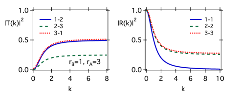
Figure 2: Transmission and reflection probabilities for Y-junction with pure $\delta$ type connection between all lines. In the left side, solid line represents $|{\cal T}_{12}(k)|^{2}$, dashed line $|{\cal T}_{23}(k)|^{2}$, and dotted line $|{\cal T}_{31}(k)|^{2}$. In the right, solid line represents $|{\cal R}_{1}(k)|^{2}$, dashed line $|{\cal R}_{2}(k)|^{2}$, and dotted lin $|{\cal R}_{3}(k)|^{2}$. Parameter values $t_{2}=t_{3}=1/\sqrt{2}$, $s=2$ are used in (27). Two identical lines are drawn with slight offsets for better viewing.

The transmission amplitudes for this case are given by

$${\cal T}_{31}(k)=\frac{2t_{3}^{*}k}{{\textrm{i}}s+(1+t_{2}^{*}t_{2}+t_{3}^{*}t_{3})k},$$

$${\cal T}_{12}(k)=\frac{2t_{2}k}{{\textrm{i}}s+(1+t_{2}^{*}t_{2}+t_{3}^{*}t_{3})k},$$

$${\cal T}_{23}(k)=\frac{2t_{2}^{*}t_{3}k}{{\textrm{i}}s+(1+t_{2}^{*}t_{2}+t_{3}^{*}t_{3})k}.$$ (27)

which has the length scale $(1+t_{2}^{*}t_{2}+t_{3}^{*}t_{3})/s$. Below this length scale, the transmission coefficients show the high-wave number pass filtering behavior

$${\cal T}_{ij}(0)=0,\quad{\cal T}_{ij}(k)=Const.\ \ {\rm as}\ k\to 0,$$ (28)

which is a hallmark of pure $\delta$ connections between all branches (See Figs. 1 and 2).

4.3 rank($B$)=2

The ST form $B\Psi^{\prime}=-A\Psi$ now reads

$$\begin{pmatrix}1&0&t_{1}\cr 0&1&t_{2}\cr 0&0&0\end{pmatrix}\begin{pmatrix}\varphi^{\prime}_{1}\cr\varphi^{\prime}_{2}\cr\varphi^{\prime}_{3}\end{pmatrix}=\begin{pmatrix}s_{11}&s_{12}&0\cr s^{*}_{12}&s_{22}&0\cr-t_{1}^{*}&-t_{2}^{*}&1\end{pmatrix}\begin{pmatrix}\varphi_{1}\cr\varphi_{2}\cr\varphi_{3}\end{pmatrix}.$$ (29)

The relation (4) becomes $\mathrm{rank}(A)=1+\mathrm{rank}(S)$. We have three possibilities:

4.3.1 rank($B$)=2, rank($A$)=1

This corresponds to $\mathrm{rank}(S)=0$. We have $s_{11}=s_{12}=s_{22}=0$ in (29). This situation represents a scale invariant interaction between lines 1–3, described by $\varphi^{\prime}_{1}=-t_{3}\varphi^{\prime}_{3}$, and a scale invariant interaction between lines 2–3, described by $\varphi^{\prime}_{2}=-t_{3}\varphi^{\prime}_{3}$.

4.3.2 rank($B$)=2, rank($A$)=2

Suppose that the rank of the sub-matrix $S$ is one, namely top two raws of the RHS are linearly dependent to each other. We can write (29) in the form

$$\begin{pmatrix}1&0&t_{1}\cr 0&1&t_{2}\cr 0&0&0\end{pmatrix}\begin{pmatrix}\varphi^{\prime}_{1}\cr\varphi^{\prime}_{2}\cr\varphi^{\prime}_{3}\end{pmatrix}=\begin{pmatrix}s&cs&0\cr c^{*}s&c^{*}cs&0\cr-t_{1}^{*}&-t_{2}^{*}&1\end{pmatrix}\begin{pmatrix}\varphi_{1}\cr\varphi_{2}\cr\varphi_{3}\end{pmatrix}.$$ (30)

Interestingly, we can reverse the role of $A$ and $B$ in the following manner. We now write (30) in the form

$$\begin{pmatrix}1&t_{1}&0\cr 0&0&0\cr 0&t_{2}&1\end{pmatrix}\begin{pmatrix}\varphi^{\prime}_{1}\cr\varphi^{\prime}_{3}\cr\varphi^{\prime}_{2}\end{pmatrix}=\begin{pmatrix}s&0&cs\cr-t_{1}^{*}&1&-t_{2}^{*}\cr c^{*}s&0&c^{*}cs\end{pmatrix}\begin{pmatrix}\varphi_{1}\cr\varphi_{3}\cr\varphi_{2}\end{pmatrix}.$$ (31)

Multiplying the both sides by

$$\begin{pmatrix}1/s&0&0\cr t_{1}^{*}/s&1&0\cr-c^{*}&0&1\end{pmatrix},$$ (32)

we obtain a reverse ST form $-B\Psi^{\prime}=A\Psi$ as

$$\begin{pmatrix}{\bar{s}}&{\bar{c}}{\bar{s}}&0\cr{\bar{c}}^{*}{\bar{s}}&{\bar{c}}^{*}{\bar{c}}s&0\cr-{\bar{t}}_{1}^{*}&-{\bar{t}}_{3}^{*}&1\end{pmatrix}\begin{pmatrix}\varphi^{\prime}_{1}\cr\varphi^{\prime}_{3}\cr\varphi^{\prime}_{2}\end{pmatrix}=\begin{pmatrix}1&0&{\bar{t}}_{1}\cr 0&1&{\bar{t}}_{3}\cr 0&0&0\end{pmatrix}\begin{pmatrix}\varphi_{1}\cr\varphi_{3}\cr\varphi_{2}\end{pmatrix},$$ (33)

with ${\bar{s}}=1/s$, ${\bar{c}}=t_{1}$, ${\bar{t}_{1}}=c$, and ${\bar{t}}_{3}=ct_{1}^{*}-t_{2}^{*}$. Note that two forms (30) and (33) are dual to each other, and that this case can be also viewed as having ${\rm rank}(A)=2$ and ${\rm rank}({\bar{S}})=1$, as well as ${\rm rank}(B)=2$ and ${\rm rank}(S)=1$.

It is instructive to look at the transmission amplitudes, which, for this case, are given by

$$\!\!\!\!\!\!\!\!{\cal T}_{31}(k)=\frac{2t_{1}^{*}k+2{\textrm{i}}c^{*}s(ct_{1}^{*}-t_{2}^{*})}{D_{1}k+{\textrm{i}}sD_{0}},$$ (34)

$$\!\!\!\!\!\!\!\!{\cal T}_{12}(k)=\frac{-2t_{2}^{*}t_{1}k-2{\textrm{i}}cs}{D_{1}k+{\textrm{i}}sD_{0}},$$

$$\!\!\!\!\!\!\!\!{\cal T}_{23}(k)=\frac{2t_{2}k-2{\textrm{i}}s(c^{*}t_{1}-t_{2})}{D_{1}k+{\textrm{i}}sD_{0}}.$$

where we set

$$\!\!\!\!\!\!\!\!D_{0}=1+c^{*}c+(ct_{1}^{*}-t_{2}^{*})(c^{*}t_{1}-t_{2}),$$

$$\!\!\!\!\!\!\!\!D_{1}=1+t_{1}^{*}t_{1}+t_{2}^{*}t_{2}.$$ (35)

Two special cases are noteworthy, at which we shall look in detail.

Figure 3: Mixed type vertex coupling obtained from ST form with ${\rm rank}(B)=2$ and ${\rm rank}(A)=2$. The $\delta$–$\delta$–$\delta^{\prime}$ (left) and $\delta^{\prime}$–$\delta^{\prime}$–$\delta$ (right) type connection are obtained from conditions ${\bar{t}}_{3}=0$ and $t_{2}=0$, respectively.

4.3.2.1   $\delta$-$\delta$-$\delta^{\prime}$ type
Let us suppose for now, that we have $ct_{1}^{*}-t_{2}^{*}(={\bar{t}}_{3}^{*})=0$. This results in ${\cal T}_{31}(0)={\cal T}_{23}(0)=0$, indicating the presence of two pure $\delta$-like connections between lines $3-1$, and between $2-3$. When further condition $s\gg t_{1}^{*}t_{1}$ and $c\neq 0$ are met, we have $T_{12}(k)=Const.$ as $k\to 0$ and $T_{12}(\infty)\approx 0$, signifying the pure $\delta^{\prime}$-like connection between lines $1-2$. The same conclusion is drawn from the consideration of connection conditions which reads

$$\!\!\!\!\!\!\!\!\!\!\!\!\!\!\!\!\!\!\!\!\!\!\!\!\frac{1}{t_{1}}\varphi^{\prime}_{1}+\varphi^{\prime}_{3}=\frac{1}{t_{2}}\varphi^{\prime}_{2}+\varphi^{\prime}_{3}=\frac{s}{t_{1}^{*}t_{1}}\varphi_{3}$$

$$\!\!\!\!\varphi_{3}=t_{1}^{*}\varphi_{1}+t_{2}^{*}\varphi_{2}$$

$$\!\!\!\!\frac{1}{t_{1}}\varphi^{\prime}_{1}=\frac{1}{t_{2}}\varphi^{\prime}_{2}.$$ (36)

The last equation, which is not independent of the first three, is shown to display the pure $\delta^{\prime}$-like interaction between the half lines $1$ and $2$, ammended by the Fülöp-Tsutsui scaling by factor $t_{1}/t_{2}$. The first two equations clearly show the fact that the connections between the half lines $2$ and $3$, and between $3$ and $1$ are pure $\delta$-like (See Fig. 3, left, and Fig. 4).

4.3.2.2   $\delta^{\prime}$-$\delta^{\prime}$-$\delta$ type
Let us now suppose, in place of previous conditions, that we have $t_{2}=0$ and $t_{1}\neq 0$. We then have ${\cal T}_{12}(\infty)={\cal T}_{23}(\infty)=0$, ${\cal T}_{12}(k)=Const.\neq 0$ and ${\cal T}_{23}(k)=Const.\neq 0$ as we let $k\to 0$, indicating the presence of two pure $\delta^{\prime}$-like connections between lines $1-2$ and between $2-3$. With further assumption $c\ll 1$, we have ${\cal T}_{31}(0)\approx 0$, signifying the pure $\delta$-like connection between lines $3-1$ (See Fig. 3, right, and Fig. 5). These facts are again clearly visible in the following expressions for the boundary condition;

$$\!\!\!\!\!\!\!\!\!\!\!\!\!\!\!\!\!\!\!\!\!\!\!\!\frac{1}{c}\varphi_{1}+\varphi_{2}=\frac{1}{ct_{1}^{*}}\varphi_{3}+\varphi_{2}=\frac{1}{sc^{*}c}\varphi^{\prime}_{2},$$

$$\!\!\!\!\varphi^{\prime}_{2}=c^{*}\varphi^{\prime}_{1}+c^{*}t_{1}\varphi^{\prime}_{3},$$

$$\!\!\!\!t_{1}^{*}\varphi_{1}=\varphi_{3}.$$ (37)

Thus we have shown that this case corresponds to a mixture of $\delta$ and $\delta^{\prime}$ connections including two pure connections $\delta-\delta-\delta^{\prime}$ and $\delta^{\prime}-\delta^{\prime}-\delta$ as two limiting cases.

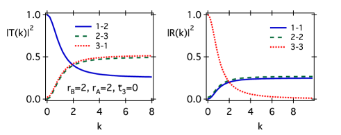
Figure 4: Transmission and reflection probabilities for Y-junction with $\delta$–$\delta$–$\delta^{\prime}$ type connection. In the left side, solid line represents $|{\cal T}_{12}(k)|^{2}$, dashed line $|{\cal T}_{23}(k)|^{2}$, and dotted line $|{\cal T}_{31}(k)|^{2}$. In the right, solid line represents $|{\cal R}_{1}(k)|^{2}$, dashed line $|{\cal R}_{2}(k)|^{2}$, and dotted lin $|{\cal R}_{3}(k)|^{2}$. Parameter values $t_{1}=t_{2}=1/\sqrt{2}$, $s_{11}=s_{12}=s_{22}=1$ are used in (29). Two identical lines are drawn with slight offsets for better viewing.

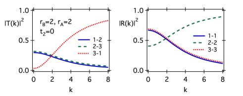
Figure 5: Transmission and reflection probabilities for Y-junction with $\delta$–$\delta^{\prime}$–$\delta^{\prime}$ type connection. Parameter values $t_{1}=1/3,t_{2}=0$, $s_{11}=6,s_{12}=2,s_{22}=2/3$ are used in (29).

4.3.3 rank($B$)=2, rank($A$)=3

When the rank of the matrix $A$ is three (thus giving $\mathrm{rank}(S)=2$), we have rather general combination of $\delta$ and $\delta^{\prime}$ interactions between each pair of half lines. Let us look at the transmission amplitudes, which are given by

$$\!\!\!\!\!\!\!\!\!\!\!\!\!\!{\cal T}_{31}(k)=\frac{2t_{1}^{*}k^{2}+2{\textrm{i}}(s_{22}t_{1}^{*}-s_{12}^{*}t_{2}^{*})k}{k^{2}E_{2}+{\textrm{i}}kE_{1}+E_{0}},$$

$$\!\!\!\!\!\!\!\!\!\!\!\!\!\!{\cal T}_{12}(k)=\frac{-2t_{2}^{*}t_{1}k^{2}-2{\textrm{i}}s_{12}k}{k^{2}E_{2}+{\textrm{i}}kE_{1}+E_{0}},$$

$$\!\!\!\!\!\!\!\!\!\!\!\!\!\!{\cal T}_{23}(k)=\frac{2t_{2}k^{2}-2{\textrm{i}}(s_{12}^{*}t_{1}-s_{11}t_{2})k}{k^{2}E_{2}+{\textrm{i}}kE_{1}+E_{0}},$$ (38)

where we set

$$\!\!\!\!\!\!\!\!\!\!\!\!\!\!E_{0}=-\det[S],$$

$$\!\!\!\!\!\!\!\!\!\!\!\!\!\!E_{1}={\rm tr}[S]+s_{22}t_{1}^{*}t_{1}-s_{12}t_{1}^{*}t_{2}-s_{12}^{*}t_{2}^{*}t_{1}+s_{11}t_{2}^{*}t_{2}$$

$$\!\!\!\!\!\!\!\!\!\!\!\!\!\!E_{2}=1+t_{1}^{*}t_{1}+t_{2}^{*}t_{2}.$$ (39)

The guaranteed presence of $\delta$-like connection between all lines can be seen from the zero energy blockade ${\cal T}_{ij}(0)=0$ for all $i$ and $j$. The presence or absence of $\delta^{\prime}$-like component is controlled by $t_{i}$ since we have ${\cal T}_{31}(\infty)\propto t_{1}^{*}$, ${\cal T}_{12}(\infty)\propto t_{2}^{*}t_{1}$ and ${\cal T}_{23}(\infty)\propto t_{2}$. A numerical example of this case is shown in Fig. 6.

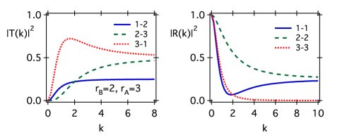
Figure 6: Transmission and reflection probabilities for Y-junction with ${\rm rank}(B)=2$, ${\rm rank}(A)=3$. Parameter values $t_{1}=t_{2}=1/\sqrt{2}$, $s_{11}=s_{12}=1$, $s_{22}=-2$ are used in (29).

4.4 rank($B$)=3

We have the ST form

$$\begin{pmatrix}\varphi^{\prime}_{1}\cr\varphi^{\prime}_{2}\cr\varphi^{\prime}_{3}\end{pmatrix}=\begin{pmatrix}s_{11}&s_{12}&s_{13}\cr s^{*}_{12}&s_{22}&s_{23}\cr s^{*}_{13}&s^{*}_{23}&s_{33}\end{pmatrix}\begin{pmatrix}\varphi_{1}\cr\varphi_{2}\cr\varphi_{3}\end{pmatrix}.$$ (40)

From (3), we have $A=S$, and thus $\mathrm{rank}(A)=\mathrm{rank}(S)$. We have four possibilities:

4.4.1 rank($B$)=3, rank($A$)=0

This corresponds to $\mathrm{rank}(S)=0$, and the boundary condition becomes

$$\Psi^{\prime}=0$$ (41)

which is the disjoint Neumann condition $\varphi^{\prime}_{1}$ $=\varphi^{\prime}_{2}$ $=\varphi^{\prime}_{3}$ $=0$.

4.4.2 rank($B$)=3, rank($A$)=1

When the rank of the matrix $A$ is one, namely three rows of the RHS are linearly dependent on each other, we have

$$\begin{pmatrix}\varphi^{\prime}_{1}\cr\varphi^{\prime}_{2}\cr\varphi^{\prime}_{3}\end{pmatrix}=\begin{pmatrix}s&cs&ds\cr c^{*}s&c^{*}cs&c^{*}ds\cr d^{*}s&d^{*}cs&d^{*}ds\end{pmatrix}\begin{pmatrix}\varphi_{1}\cr\varphi_{2}\cr\varphi_{3}\end{pmatrix}.$$ (42)

Multiplying the both sides by

$$\begin{pmatrix}1/s&0&0\cr-c^{*}&1&0\cr-d^{*}&0&1\end{pmatrix},$$ (43)

we arrive at a reverse ST form as

$$\begin{pmatrix}{\bar{s}}&0&0\cr-c^{*}&1&0\cr-d^{*}&0&1\end{pmatrix}\begin{pmatrix}\varphi^{\prime}_{1}\cr\varphi^{\prime}_{2}\cr\varphi^{\prime}_{3}\end{pmatrix}=\begin{pmatrix}1&c&d\cr 0&0&0\cr 0&0&0\end{pmatrix}\begin{pmatrix}\varphi_{1}\cr\varphi_{2}\cr\varphi_{3}\end{pmatrix},$$ (44)

with ${\bar{s}}=1/s$. We have $c^{*}d^{*}\varphi^{\prime}_{1}=d^{*}\varphi^{\prime}_{2}=c^{*}\varphi^{\prime}_{3}$, and $\varphi_{1}+c\varphi_{2}+d\varphi_{3}={\bar{s}}\varphi^{\prime}_{1}$, signifying the generalized pure $\delta^{\prime}$ interaction [8] ammended by the Fülöp-Tsutsui scaling. This is also evident from the transmission amplitudes, which are given by

$${\cal T}_{31}(k)=\frac{2d^{*}s}{-{\textrm{i}}k+s(1+c^{*}c+d^{*}d)},$$

$${\cal T}_{12}(k)=\frac{2cs}{-{\textrm{i}}k+s(1+c^{*}c+d^{*}d)},$$

$${\cal T}_{23}(k)=\frac{2c^{*}ds}{-{\textrm{i}}k+s(1+c^{*}c+d^{*}d)}.$$ (45)

The formulae imply ${\cal T}_{ij}(\infty)=0$ and ${\cal T}_{ij}(k)=Const.$ as $k\to 0$ (See Figs. 7 and 8).

Figure 7: Pure $\delta^{\prime}$ type connection between all lines, obtained from ST form with ${\rm rank}(B)=3$ and ${\rm rank}(A)=1$.

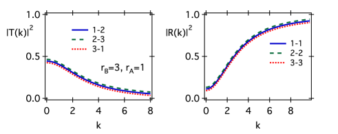
Figure 8: Transmission and reflection probabilities for Y-junction with pure $\delta^{\prime}$ type connection between all lines. Parameter values $s_{11}=s_{12}=s_{13}=s_{22}=s_{23}=s_{33}=1$ are used in (40).

4.4.3 rank($B$)=3, rank($A$)=2

When the rank of the matrix $A$ is two, and thus that of $S$ is two, the last row of RHS of (40) is equal to some combination of the first two. We then have

$$\begin{pmatrix}\varphi^{\prime}_{1}\cr\varphi^{\prime}_{2}\cr\varphi^{\prime}_{3}\end{pmatrix}=\begin{pmatrix}s&q&\!\!\!\!cs+dq\cr q^{*}&r&\!\!\!\!cq^{*}+dr\cr c^{*}s+d^{*}q^{*}\!&\!c^{*}q+d^{*}r\!\!&f\end{pmatrix}\begin{pmatrix}\varphi_{1}\cr\varphi_{2}\cr\varphi_{3}\end{pmatrix}$$ (46)

with $f=c^{*}cs+c^{*}dq+d^{*}cq^{*}+d^{*}dr$. Multiplying both sides by

$$\begin{pmatrix}r/(sr-q^{*}q)&-q/(sr-q^{*}q)&0\cr-q^{*}/(sr-q^{*}q)&s/(sr-q^{*}q)&0\cr-c^{*}&-d^{*}&1\end{pmatrix},$$ (47)

we obtain a reverse ST form

$$\begin{pmatrix}{\bar{s}}&{\bar{q}}&0\cr{\bar{q}}^{*}&{\bar{r}}&0\cr-{\bar{t}^{*}_{1}}&-{\bar{t}^{*}_{2}}&1\end{pmatrix}\begin{pmatrix}\varphi^{\prime}_{1}\cr\varphi^{\prime}_{2}\cr\varphi^{\prime}_{3}\end{pmatrix}=\begin{pmatrix}1&0&{\bar{t}}_{1}\cr 0&1&{\bar{t}}_{2}\cr 0&0&0\end{pmatrix}\begin{pmatrix}\varphi_{1}\cr\varphi_{2}\cr\varphi_{3}\end{pmatrix},$$ (48)

with identification ${\bar{s}}=r/(sr-q^{*}q)$, ${\bar{q}}=-q/(sr-q^{*}q)$, ${\bar{r}}=s/(sr-q^{*}q)$, ${\bar{t}}_{1}=c$, and ${\bar{t}}_{2}=d$.

This is obviously dual to the case of $m=2$, ${\rm rank}(S)=2$. Now the presence of $\delta^{\prime}$-like connection between all lines are guaranteed, and the presence or absence of $\delta$-like component is controlled by $c$ and $d$. The transmission amplitudes, given by

$$\!\!\!\!\!\!\!\!\!\!\!\!{\cal T}_{31}(k)=\frac{2{\textrm{i}}k(c^{*}s+d^{*}q^{*})-2c^{*}(sr-q^{*}q)}{k^{2}+{\textrm{i}}kF_{1}+F_{0}},$$

$$\!\!\!\!\!\!\!\!\!\!\!\!{\cal T}_{12}(k)=\frac{2{\textrm{i}}kq+2cd^{*}(sr-q^{*}q)}{k^{2}+{\textrm{i}}kF_{1}+F_{0}},$$

$$\!\!\!\!\!\!\!\!\!\!\!\!{\cal T}_{23}(k)=\frac{2{\textrm{i}}k(cq^{*}+dr)-2d(sr-q^{*}q)}{k^{2}+{\textrm{i}}kF_{1}+F_{0}},$$ (49)

where we set

$$\!\!\!\!\!\!\!\!\!\!\!\!F_{0}=-(sr-q^{*}q)(1+c^{*}c+d^{*}d),$$

$$\!\!\!\!\!\!\!\!\!\!\!\!F_{1}=s+r+c^{*}cs+c^{*}dq+d^{*}cq^{*}+d^{*}dr,$$ (50)

corroborate this assertion with high energy blockade ${\cal T}_{ij}(\infty)=0$ for all $i$ and $j$, and also with the zero energy expressions ${\cal T}_{31}(0)\propto c^{*}$, ${\cal T}_{12}(0)\propto d^{*}c$ and ${\cal T}_{23}(0)\propto d$. A numerical example of this case is shown in Fig. 9.

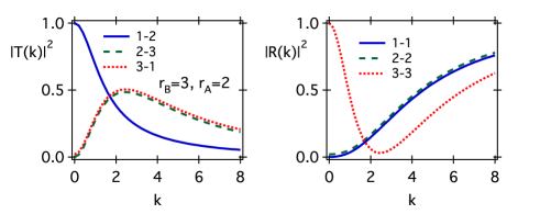
Figure 9: Transmission and reflection probabilities for Y-junction with ${\rm rank}(B)=3$, ${\rm rank}(A)=2$. Parameter values $s_{11}=s_{12}=s_{22}=s_{33}=1$, $s_{13}=s_{23}=2$ are used in (40).

4.4.4 rank($B$)=3, rank($A$)=3

When the ranks of the matrices $A$ and $B$ are both equal to $n=3$, we have the generic connection condition for a quantum particle residing on a joint three lines, namely the combinations of $\delta$ and $\delta^{\prime}$ interactions.

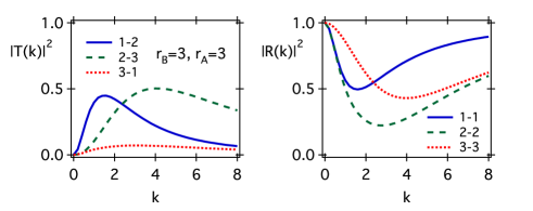
Figure 10: Transmission and reflection probabilities for Y-junction with ${\rm rank}(B)=3$, ${\rm rank}(A)=3$, the generic condition. In the left side, solid line represents $|{\cal T}_{12}(k)|^{2}$, dashed line $|{\cal T}_{23}(k)|^{2}$, and dotted line $|{\cal T}_{31}(k)|^{2}$. In the right, solid line represents $|{\cal R}_{1}(k)|^{2}$, dashed line $|{\cal R}_{2}(k)|^{2}$, and dotted lin $|{\cal R}_{3}(k)|^{2}$. Parameter values $s_{11}=-1/3$, $s_{12}=-1$, $s_{13}=1$, $s_{22}=1$, $s_{23}=-3$, $s_{33}=-4$ are used in (40).

Let us look at the transmission amplitudes, which are given by

$${\cal T}_{ij}(k)=\frac{-2{\textrm{i}}k^{2}s_{ij}+2k\det[{\cal S}_{ji}]}{k^{3}+{\textrm{i}}k^{2}{\rm tr}[S]-k\sum_{i}\det[{\cal S}_{ii}]-{\textrm{i}}\det[S]}.$$ (51)

We have ${\cal T}_{ij}(0)={\cal T}_{ij}(\infty)=0$ for all $i\neq j$ signifying the guaranteed presence of both $\delta$-like and $\delta^{\prime}$-like components in the connections between all lines.

This expression, along with the analogous expression for $n=r_{A}=r_{B}=2$ case, invites an easy straightforward extension to general $n$. A numerical example of this case is shown in Fig. 10.

5 Conclusion

Our main finding in this article on quantum Y-junction is the fact that the couplings between each pair of outgoing lines are individually tunable. The ST form of vertex boundary condition, which gives the prescription for minimal construction of singular vertex as a limit of finite potentials, is also found to be instrumental in identifying the type of coupling between all pairs of outgoing lines. Crucial quantity to identify the physics of singular vertex is to be found in the rank of matrices $A$ and $B$ appearing in the ST form.

Specifically, the pure $\delta$-type coupling is constructed from ${\rm rank}(B)=1$ boundary condition, while the pure $\delta^{\prime}$-type coupling is constructed from ${\rm rank}(A)=1$.

Boundary condition corresponding to ST form for $n=3$ with ${\rm rank}(A)={\rm rank}(B)=2$ is identified as containing Y-junction with both $\delta$–$\delta$–$\delta^{\prime}$ type and $\delta^{\prime}$–$\delta^{\prime}$–$\delta$ type singular verteces as limiting cases of parameter values ${\bar{t}_{i}}=0$ and $t_{i}=0$, respectively. Spectral filtering of quantum waves is achieved by these types of singular vertices.

The extension of our treatment to quantum singular vertex of degree $n=4$, or ”X-junction”, and then to that with higher $n$ appears tedious, but is within reach once the need of detail analysis is required as a model of quantum single electron devices. We hope that this work becomes a stepping stone for such extensions. Obviously, the experimental realization and demonstration with quantum wires and quantum dots are highly desired. Designing real-world approximation for singular vertex of quantum graph then becomes crucial [7, 9, 10, 11].

We acknowledge the financial support by the Ministry of Education, Culture, Sports, Science and Technology, Japan (Grant number 21540402), and also by the Czech Ministry of Education, Youth and Sports (Project LC06002).

References

[1]
P. Exner, J.P. Keating, P. Kuchment, T. Sunada, A. Teplyaev, eds.:
Analysis on Graphs and Applications, Proceedings of a Isaac
Newton Institute programme, January 8–June 29, 2007; 670 p.; AMS
“Proceedings of Symposia in Pure Mathematics” Series, vol. 77,
Providence, R.I., 2008.
[2]
V. Kostrykin, R. Schrader,
J. Phys. A: Math. Gen. 32 (1999) 595-630.
[3]
M. Harmer, J. Phys. A: Math. Gen. 33 (2000), 9193-9203.
[4]
V. Kostrykin, R. Schrader, Fortschr. Phys. 48 (2000), 703-716.
[5]
T. Fülöp and I. Tsutsui,
Phys. Lett. A264 (2000)
366–374.
[6]
I. Tsutsui, T. Fülöp and T. Cheon,
J. Math. Phys. 42 (2001)
5687-5697.
[7]
T. Cheon, P. Exner and O. Turek,
arXiv.org: 0908.2679 (2009).
[8]
P. Exner, J. Phys. A: Math. Gen. 29 (1996) 87-102.
[9]
T. Cheon and T. Shigehara, Phys. Lett. A 243 (1998) 111-116.
[10]
P. Exner and O. Turek,
Rev. Math. Phys. 19 (2007) 571-606.
[11]
P. Kuchment,
Waves and Random Media 14 (2004) S107-S128.