Uncovering delayed patterns in noisy and irregularly sampled time series: an astronomy application

Abstract

We study the problem of estimating the time delay between two signals representing delayed, irregularly sampled and noisy versions of the same underlying pattern. We propose and demonstrate an evolutionary algorithm for the (hyper)parameter estimation of a kernel-based technique in the context of an astronomical problem, namely estimating the time delay between two gravitationally lensed signals from a distant quasar. Mixed types (integer and real) are used to represent variables within the evolutionary algorithm. We test the algorithm on several artificial data sets, and also on real astronomical observations of quasar Q0957+561. By carrying out a statistical analysis of the results we present a detailed comparison of our method with the most popular methods for time delay estimation in astrophysics. Our method yields more accurate and more stable time delay estimates: for Q0957+561, we obtain 419.6 days between images A and B. Our methodology can be readily applied to current state-of-the-art optical monitoring data in astronomy, but can also be applied in other disciplines involving similar time series data.

, , , ,

1 Introduction

The estimation of time delay, the delay between arrival times of two signals that originate from the same source but travel along different paths to the observer, is a real-world problem in Astronomy. A time series to be analysed could, for instance, represent the repeated measurement, over many months or years, of the flux of radiation (optical light or radio waves) from a very distant quasar, a very bright source of light usually a few billion light-years away. Some of these quasars appear as a set of multiple nearby images on the sky, due to the fact that the trajectory of light coming from the source gets bent as it passes a massive galaxy on the way (the “lens”), and, as a result, the observer receives the light from various directions, resulting in the detection of several images [29, 46]. This phenomenon is called gravitational lensing, and is a natural consequence of a prediction of the General theory of Relativity, which postulates that massive objects distort space-time and thus cause the bending of trajectories of light rays passing near them. Quasars are variable sources, and the same sequence of variations is detected at different times in the different images, according to the travel time along the various paths. The time delay between the signals depends on the mass of the lens, and thus it is the most direct method to measure the distribution of matter in the Universe, which is often dark [43, 29].

In this scenario, the underlying pattern in time of emitted flux intensities from a quasar gets delayed and corrupted by all kinds of noise processes. For example, astronomical time series are not only corrupted by observational noise, but they are also typically irregularly sampled with possibly large observational gaps (missing data) [33, 40, 32, 27]. This is due to practical limitations of observation such as equipment availability, weather conditions, the brightness of the moon, among many other factors [17]. Over a hundred systems of lensed quasars are currently known, and about 10 of these have been monitored for long periods, and in some of these cases, the measurement of a time delay has been claimed. Here we focus on Q0957+561, the first multiply-imaged quasar to be discovered [51]. This source, which has a pair of images (here referred to as A and B), has been monitored for over twenty years, and despite numerous claims, a universally agreed value for the time delay in this system has not emerged [30, 14].

In an earlier paper, we presented an analysis of repeated radio observations, along with simulated data generated according to the properties of these observations [14], to show that a kernel-based approach can improve upon the currently popular methods of estimating time delays from real astronomical data. The more common form of observations, however, employs optical telescopes for monitoring known multiply-imaged sources, and these observations have inherent problems that require the modification of our previous approach. Here we present a largely modified approach that outperforms on optical datasets our previous appraoch, as well as alternative approaches in use in astrophysics.

Here we introduce a novel evolutionary algorithm (EA) to estimate the parameters of a model-based method for time delay estimation. The EA uses, as a fitness function, the mean squared error (MSE_CV) given by cross-validation on observed data, and also performs a novel regularisation procedure based on singular value decomposition (SVD). Our population is also represented by mixed types, integers and reals.

The contribution of this paper is in several directions: i) an evolutionary algorithm has been introduced to form a novel hybridisation with our kernel method, ii) a principled automatic method has been proposed to estimate the time delay, kernel width, and SVD regularisation parameters, iii) the application of EA driven by a model based formulation to a real-world problem, and iv) we carefully study statistical significance of the results on different data.

Our EA is an evolutionary optimisation technique in presence of uncertainties [28] and missing data with mixed representation – through two linked populations, each devoted to one particular data type. The parameters to optimise come from a kernel machine. We do parameter optimisation and model selection at the same time. This approach can be applied to other problems, not only time series from gravitational lensing. For instance, the missing data problems cover those cases where instrumental equipment fails, observations are incorrectly recorded, sociological factors are involved, etc. Therefore, the data are unevenly sampled, which restricts the use of Fourier analysis [42](§13.8). Problems with noisy and missing data occur in almost all sciences, where the data availability is influenced by what is easy or feasible to collect (e.g., see [12, 6]).

We compare the performance of our EA in several ways:

1. The performance of our method is assessed against that of two of the most popular methods in the astrophysical literature [50, 18, 33, 11, 22], i.e., (a) the Dispersion spectra method [36, 37, 35, 14] and (b) a scheme based on the structure function of the intrinsic variability of the source, here referred to as the PRH method [41].

2. Because the true time delay of observed fluxes from quasars is not known, we assess the performance of algorithms in a controlled series of experiments, where artificially generated data with known delays are used. We employ three kinds of artificial data sets: large scale data [14], PRH data [41, 14] and Wiener data (as outlined in [23, 24]).

3. To justify our EA, an analogous non-evolutionary model-based approach (K-V) is also employed in this paper.

Our statistical analysis shows that the results from our EA are more accurate and significant than state-of-the-art methods. We use our EA as well as a (1+1)-ES algorithm [45] on actual astronomical observations, where the twin images were observed over several years with optical telescopes [30].

The remainder of this paper is organised as follows: the data under analysis is described in §2. The kernel approach is outlined in §3, and the EA is presented in §4. The results and our conclusions are in §5 and §6 respectively. Finally, our future work is presented in §7.

2 Data

2.1 Optical Data

In this paper, we use optical observations of the two images of the quasar Q0957+561, from a monitoring program at the Apache Point Observatory, New Mexico, USA [30]. This data set has 97 observations, where, in each observation, fluxes are measured of all the multiple images of the source, in the $g$-band (a standard yellow-green filter), from December 1994 to July 1996.

The observed time series (here called light curves) are given in Table 1, where the Time column, representing the time of observation (note that it is irregularly sampled), is given in Julian days (JD, defined as the number of days since Noon GMT on January 1, 4713 BC). The fluxes observed from images A and B are given in the astronomical unit of magnitude (mag $m$), defined as $m=-2.5\,\log_{10}\,f$, where $f$ is the flux measured when observed through a green filter ($g$-band). In Fig. 1, the time series are shown. The measurement errors, which are standard deviations (std) of the flux measurement, are given in the Table 1 as Error A and Error B; these are the error bars. The source was monitored nightly, but many observations were missed due to cloudy weather and telescope scheduling. The big gap in Fig. 1 is an intentional gap in the nightly monitoring, since a delay of about 400 days, the pattern, was known ‘a priori’ – monitoring programs on this quasar started in 1979. Therefore, the peak in the light curve of image A, between 700 and 800 days, corresponds to the peak in that of image B between 1,100 and 1,200 days.

Table 1: Optical data: Q0957+561 observed in the $g$-band, from [30]

Time	Image A	Error A	Image B	Error B
(days)	(mag)		(mag)
689.009	16.9505	0.0152	16.8010	0.0152
691.007	16.9439	0.0111	16.7957	0.0111
695.001	16.9356	0.0090	16.7949	0.0090
…	…	…	…	…
1253.672	17.0544	0.0084	16.9206	0.0084
1266.665	17.0544	0.0205	16.9808	0.0205
1268.642	17.0798	0.0170	16.9261	0.0170
1270.652	17.0928	0.0145	16.9597	0.0119

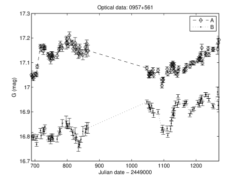
Figure 1: Observations of the brightness of the doubly-imaged quasar Q0957+561, in the $g$-band, as a function of time (Top: Image A; Bottom: Image B, see Table 1). The time is measured in days (Julian days–2,449,000 days).

2.2 Artificial Data

Since the definite time delay for the Q0957+561 is unknown, one cannot test the accuracy of methods through real data. Therefore, many attempts have been made to generate synthetic data in order to test the performance of methods (e.g. [41, 39, 7, 17, 23, 24]). Below we describe three kinds of artificial data sets that we have used, representing the major classes of data sets used by others: large scale data, PRH data and Wiener data.

2.2.1 Large Scale Data

In this data set (DS-5), the true time delay is 5 days [15], and the true offset in brightness between image A and image B is $M=0.1$ mag. The intention here is to simulate optical observations as in Ovaldsen et al. [33]. We employ only the first five underlying functions. These data sets are irregularly sampled with three levels of noise and gaps of different size as shown in Table 2; for more details see [14, 15]. We use 50 realisations per level of noise only. Consequently, this yields 38,505 data sets (see Table 2), with 50 samples each, of which two are shown in Fig. 2.

Table 2: Simulated Large Scale Data sets

	Gap size
Noise	0	1	2	3	4	5
0%	1	10	10	10	10	10
0.036%	50	500	500	500	500	500
0.106%	50	500	500	500	500	500
0.466%	50	500	500	500	500	500
Sub-Total	151	1510	1510	1510	1510	1510
Total = 7,701 data sets per underlying function.
5 underlying functions yield 38,505 data sets.

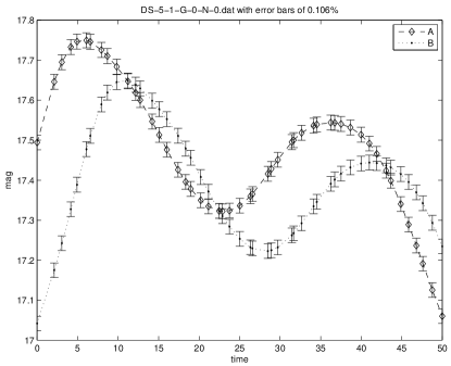
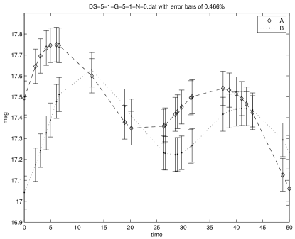
Figure 2: The simulated Large Scale Data sets, as outlined in Table 2. (a) The first underlying function (DS-5-1) without noise and no gaps. Error bars represent 0.106% of mag.(b) This data set corresponds to the same underlying function (DS-5-1), without noise, and the gap size is five (first realisation). Error bars represent 0.466% of flux.

2.2.2 PRH Data

These data sets are generated by Gaussian processes, following [41], with a fixed covariance matrix given by a structure function according to Pindor [40]. The variance representing the measurement errors is $1\times 10^{-7}$. They are highly sampled with periodic gaps [17], simulating a monitoring campaign of eight months; yielding 61 samples per time series. There are seven true delays and 100 realisations for each value of true delay [14]. Two plots are shown in Fig. 3.

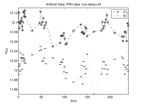
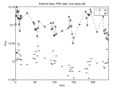
Figure 3: Examples of the simulated PRH Data. The error bars represent a variance of $1\times 10^{-7}$. (a) This is a realisation for a true delay of 34 days. Image A has been shifted upwards by 0.08 for visualisation. (b) In this realisation, the true delay is 66 days. Image A has been shifted upwards by 0.1 for visualisation.

2.2.3 Wiener Data

These data sets, generated by a Bayesian model [23], simulate three levels of noise with 225 data sets per level of noise, where each level of noise represents the variance: $0.1^{2}$, $0.2^{2}$ and $0.4^{2}$. The data are irregularly sampled and the true time delay in all cases is 35 days. Some examples are shown in Fig. 4. Each time series has 100 samples.

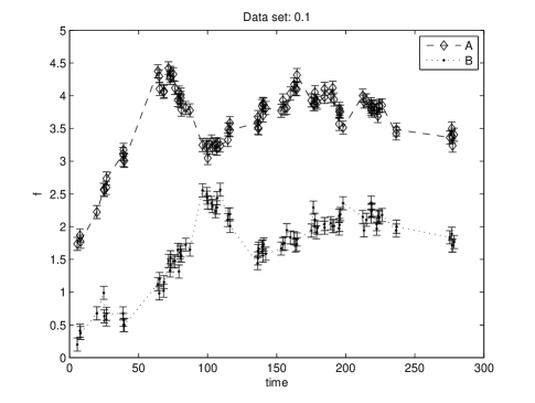
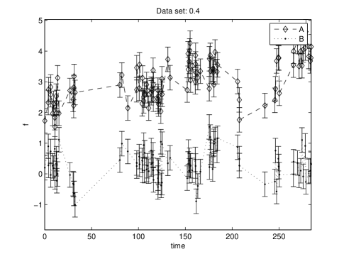
Figure 4: Simulated Wiener Data. (a) The first realisation of data sets with noise of variance $0.1^{2}$. Image A has been shifted upwards by a factor 1.5 for visualisation. (b) The first realisation of data sets with noise of variance $0.4^{2}$. Image A has been shifted upwards by 2.9 for visualisation. In each case, error bars represent the standard deviation.

3 Kernel Approach

In previous papers, [14, 15], we have introduced a kernel-based approach, and we would refer the reader to these papers for further detail, since not all derivations will be repeated here at the same level of detail. The aim of this section is to come up with the parameters to evolve in §4.

We model a pair of time series, obtained by monitoring the brightness of images A and B (see §2), as

$$\begin{array}[]{ll}x_{A}(t_{i})&=h_{A}(t_{i})+\varepsilon_{A}(t_{i})\\ x_{B}(t_{i})&=h_{B}(t_{i})\ominus M+\varepsilon_{B}(t_{i}),\end{array}$$ (1)

where $\ominus=\{\times,-\}$ denotes either multiplication or subtraction, so $M$ is either a ratio (used in radio observations, where brightness is quoted in flux units) or an offset between the two images (as in optical observations, where brightness in represented in logarithmic units). We use the latter option here. Values of the independent variable $t_{i},i=1,2,...,n$ represent discrete observation times. The observation errors $\varepsilon_{A}(t_{i})$ and $\varepsilon_{B}(t_{i})$ are modelled as zero-mean Normal distributions

$$N(0,\sigma_{A}(t_{i}))\ \ \hbox{and}\ \ N(0,\sigma_{B}(t_{i})),$$ (2)

respectively, where $\sigma_{A}(t_{i})$ and $\sigma_{B}(t_{i})$ are standard deviations. Now,

$$h_{A}(t_{i})=\sum_{j=1}^{N}\alpha_{j}K(c_{j},t_{i})$$ (3)

is the “underlying” light curve that underpins image A, whereas

$$h_{B}(t_{i})=\sum_{j=1}^{N}\alpha_{j}K(c_{j}+\Delta,t_{i})$$ (4)

is a time-delayed (by $\Delta$) version of $h_{A}(t_{i})$ underpinning image B.

The functions $h_{A}$ and $h_{B}$ are formulated within the generalised linear regression framework [25, 47]. Each function is a linear superposition of $N$ kernels $K(\cdot,\cdot)$ centred at either $c_{j}$, $j=1,2,...,N$ (function $f_{A}$), or $c_{j}+\Delta$, $j=1,2,...,N$ (function $f_{B}$). We use Gaussian kernels of width $\omega_{c}$:  for $c,t\in\Re$,

$$K(c,t)=\exp\,{\frac{-|t-c|^{2}}{\omega_{c}^{2}}}.$$ (5)

The kernel width $\omega_{c}>0$ determines the ‘degree of smoothness’ of the models $h_{A}$ and $h_{B}$ . We position kernels at the position of each observation, implying $N=n$. The width $\omega_{j}\equiv\omega_{c}$ is determined through the $k$ nearest neighbours of $c_{j}$ (equal to $t_{j}$) as

$$\omega_{j}=\sum_{d=1}^{k}(t_{j}-t_{j-d})+(t_{j+d}-t_{j})=\sum_{d=1}^{k}(t_{j+d}-t_{j-d}).$$ (6)

The weights $\vec{\alpha}$ (3)-(4) are obtained as follows [14]:

$$\vec{K}\vec{\alpha}=\vec{x},$$ (7)

where $\vec{\alpha}=(\alpha_{1},\alpha_{2},...,\alpha_{N})^{T}$,

$$\vec{K}=\left[\begin{array}[]{c}K_{A}(\cdot,\cdot)\\ \\ K_{B}(\cdot,\cdot)\end{array}\right],\ \ \ \ \ \ \ \ \vec{x}=\left[\begin{array}[]{c}x_{A}(\cdot)/\sigma_{A}(\cdot)\\ \\ x_{B}(\cdot)/\sigma_{B}(\cdot)\end{array}\right],$$ (8)

and the kernels $K_{A}(\cdot,\cdot)$, $K_{B}(\cdot,\cdot)$ have the form:

$$K_{A}(c,t)=\frac{K(c,t)}{\sigma_{A}(t)},\ \ \ \ \ \ \ K_{B}(c,t)=\frac{M\ominus K(c+\Delta,t)}{\sigma_{B}(t)}.$$ (9)

Hence,

$$\vec{\alpha}=\vec{K}^{+}\vec{x}.$$ (10)

Our aim is to estimate the time delay $\Delta$ between the temporal light curves corresponding to images A and B. Typically, $\Delta$ is estimated by a set of trial time delays in the range [$\Delta_{min}$, $\Delta_{max}$] with a specific measurement of goodness of fit [14]. In Eq. 10, the superscript “+” represents a pseudoinverse of a matrix, the pseudoinverse rather than the inverse is required because the matrix is not squared, that is, an over-determined system is involved [42].

Finally, the parameters are the time delay $\Delta$ [as given in Eqs. (3) & (4)], the variable width $k$ [as in Eq. (6)], and the regularisation parameter $\theta$ (see below).

3.1 Regularisation

In practice, the matrix $\vec{K}$ (8) may be singular because $\vec{K}$ is an over-determined system, and noisy time series (2) are involved. We therefore regularise the inversion in (10) through singular value decomposition (SVD) [14]. To avoid singularity, the most straightforward method is to find a threshold $\lambda$ for singular values [42, 21]. This means that the singular values less than $\lambda$ are set to zero, following which $\vec{K}^{+}$ (10) is obtained through SVD [42].

In other words, $\lambda$ tells us how many singular values to set to zero. Hence, for a given $\Delta$, the number of singular values to keep may vary. We illustrate this through Fig. 5, representing artificial and optical data, where $\theta$ is the number of singular values to set to zero. One can see a well defined pattern in the range $\theta=[15,27]$ ($\Delta=5$) in Fig. 5a, and $\theta=[49,72]$ ($\Delta=419$) in Fig. 5b. Thus, if one can find a proper $\lambda$ that falls in this range, then one can claim that the estimation of $\Delta$ is “robust”. But the range of this pattern may change for other $M$ and $k$ parameters, in which case there is no guarantee that the estimated $\lambda$ falls in this range. Furthermore, no matter which method is used for assessing the goodness of fit, if we test $\Delta$ in a specific range with a fixed $\lambda$, then we may come up with different values of $\theta$ – some inside the pattern, some outside, none inside, etc.

Instead of $\lambda$, we use $\theta$ as a regularisation parameter in §4. In fact, we aim to create an automatic algorithm that performs a global search for all parameters, and then finds the proper $\theta$ that falls in the pattern; with our EA, we have done this (see §4). A review of other general regularisation techniques for inverse problems can be found in Conan [13].

Figure 5: Patterns. In each relation ($\Delta$, $\theta$), the best time delay has been plotted, i.e., the best $\Delta$ (y-axis) versus the number of singular values $\theta$ set to zero (x-axis). The best time delay is found through log-likelihood [14] by evaluating time delay trials in a given range. (a) DS-5-1-G-0-N-0. This data set has no noise and no gaps; $\Delta=[0,10]$ with increments of 0.1; $M$ is set to its true value $M=0.1$ (for more details concerning these data, see §2.2.1). The pattern is at $\theta=[5,27]$, where $\Delta=5$ (true value). (b) Actual $g$-band optical observations of quasar Q0957+561, $\Delta=[400,450]$ with unitary increments. The data set is as in §2.1; $M$ was set to 0.117 [30] and $k=3$ (6). The pattern is at $\theta=[49,72]$, where $\Delta=419$ (see Tables 3 and 4, and §5).

3.2 Optimisation

The above formulation can be seen as an optimisation problem where the variables are $\Delta$, $k$ and $\theta$. Conventional gradient-based optimisation techniques cannot be used since the above kernel-based approach is not differentiable with respect to the discrete variables $k$ and $\theta$, regardless of the loss function.

Of course, since both $k$ and $\theta$ are finite range discrete variables, one can employ a brute force search driven by cross-validation. Apart form having to deal in a systematic and time-consuming manner with a huge search space, it is also not clear what the appropriate ranges and resolutions should be for parameters such as $\Delta$ or $k$. In any case, we compare our EA approach (see section §4) with a non-evolutionary kernel-based approach (K-V) for estimating time delay $\Delta$ by cross-validating $k$ and the regularisation parameter $\lambda$ [14, 15].

An example of the search landscape is in Fig 6. We use $\Delta_{min}=400$ and $\Delta_{max}=450$ with unitary increments, and $\theta=1,2,...,n$, where $n=97$. The parameter $k$ is fixed to 3, and the offset $M$ to 0.117. The real optical data ($g$-band) in §2 is used. Then, Algorithm 1 (explained later in §4) is applied to obtain the MSE_CV. Note that this landscape may change for other $k$ values and for other data sets. We can see that from $\theta=80$ to $n$ the error surface is quite complicated for simple search algorithms, e.g., gradient descent (if differentiable), hill climbing or simulated annealing search. There are also more local minima when $\theta<45$; see also Fig. 5. In the $\theta$-$\Delta$ plane, the mark (x) shows the best parameter combination; i.e., minimum MSE_CV. To smooth the surface and help the visualisation, we use a logarithmic scale.

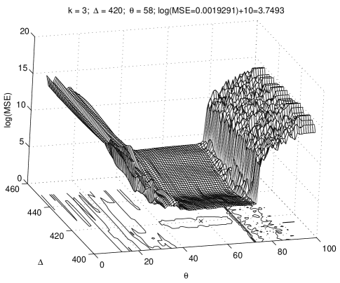
Figure 6: Example of Search Landscape. The data is from the doubly-imaged quasar Q0957+561, in the $g$-band. The parameters $k$ was fixed to 3, and the offset $M$ to 0.117. Algorithm 1 is used to obtain the log(MSE); see §4. The surface has been shifted upwards by 10 units for visualisation.

4 Evolutionary Algorithm (EA)

Following the kernel-based approach in §3, we have three parameters: (i) the time delay $\Delta$; (ii) the variable width $k$; and (iii) the number of singular values to retain $\theta$. Besides, we have a measurement of fitness (objective function), e.g. log-likelihood or a loss function, which, along with the others, gives us a third-dimensional search space $\Phi$. Therefore, we follow an EA to avoid local minima [4, 20, 48].

Let us define as our population

$$\vec{P_{\ell}}=\left[\begin{array}[]{lll | l}\Delta_{1}&\theta_{1}&k_{1}&f_{1}\\ \Delta_{2}&\theta_{2}&k_{2}&f_{2}\\ ...&...&...&...\\ \Delta_{x}&\theta_{x}&k_{x}&f_{x}\\ ...&...&...&...\\ \Delta_{p}&\theta_{p}&k_{p}&f_{p}\\ \end{array}\right],$$ (11)

where each row in $\vec{P_{\ell}}$ is a hypothesis commonly referred to as individual or chromosome, which is a set of parameters {$\Delta_{x},\theta_{x},k_{x}$}, randomly initialised.

Then we have $p$ hypotheses [31]. Each hypothesis $x$ is evaluated by $f_{x}$, which is a measure of fitness. For this, we use the mean squared error (MSE_CV) given by Cross Validation (CV), in Algorithm 1, where $T=O-V$ is the training set, $O$ is the set of all observations such as $O=\{(x_{A}(t_{i}),x_{B}(t_{i}))|i\}$, and $V$ is the validation set (the log-likelihood or simple mean squared error can also be used, but this might lead to overfitting). Thereafter, we apply artificial genetic operators such as selection, crossover, mutation and reinsertion to generate $\vec{P_{2}},...,\vec{P_{g}}$ populations. At the $g$ generation, we choose from $\vec{P_{g}}$ the best set of parameters (or individual) according to its fitness; i.e., with minimum $f_{x}$. This procedure is summarised in Algorithm 2, and the details are in §4.1.

Algorithm 1 Fitness function ($\Delta_{x}$, $k_{x}$, $\theta_{x}$)

$Blocks\leftarrow 5$
$PointsPerBlock\leftarrow n/Blocks$
for $i\leftarrow 1$ to $PointsPerBlock$
{
            Remove the $i^{th}$ observation of each block and include it
            in the validation set $V$
            Compute $\vec{h_{A}}$ and $\vec{h_{B}}$ for the training set $T$
            Get MSE_CV on the validation set $V$
            $R(i)\leftarrow$ MSE_CV
}
$f_{x}\leftarrow mean(R)$
return $f_{x}$

This process leads to artificial evolution, which is a stochastic global search and optimisation method based on the principles of biological evolution [20, 48].

Algorithm 2 Evolutionary Algorithm

(See 4.1 for details)
Initialise population $\vec{P_{1}}=[\vec{P_{1}^{1}}\ \vec{P_{1}^{2}}]$
Evaluate population $\vec{P_{1}}$ with Algorithm 1
for $\ell\leftarrow 2\ \hbox{\rm\bf to}\ g$
{
            Select $\vec{P_{\ell}^{1^{\prime}}}$ and $\vec{P_{\ell}^{2^{\prime}}}$ from $\vec{P_{1}}$
            Recombine $\vec{P_{\ell}^{1^{\prime}}}$, Recombine $\vec{P_{\ell}^{2^{\prime}}}$
            Mutate $\vec{P_{\ell}^{1^{\prime}}}$   Mutate $\vec{P_{\ell}^{2^{\prime}}}$
            Evaluate $\vec{P_{\ell}^{{}^{\prime}}}=[\vec{P_{\ell}^{1^{\prime}}}\ \vec{P_{\ell}^{2^{\prime}}}]$ with Algorithm 1
            Reinsert $\vec{P_{\ell}^{{}^{\prime}}}$ into $\vec{P_{\ell-1}}$ to obtain $\vec{P_{\ell}}$
}

4.1 Representation and Evolution Operators

We represent every population $\vec{P_{\ell}}$ in every generation $\ell=1,2,...,g$, as two linked populations of the same size $p$, $\vec{P_{\ell}}=[\vec{P_{\ell}^{1}}\ \vec{P_{\ell}^{2}}]$. The $x$-th individual in population $\vec{P_{\ell}}$ corresponds to the $x$-th individual in populations $\vec{P_{\ell}^{1}}$ and $\vec{P_{\ell}^{2}}$. The population $\vec{P^{1}_{\ell}}$ uses reals to represent $\Delta_{x}$, while $\vec{P_{\ell}^{2}}$ employs integers to represent $\theta_{x}$ and $k_{x}$. First we initialise randomly $\vec{P_{1}}$ and evaluate the population with the above fitness function. Second, we select half of the population $\vec{P_{\ell}}$ for reproduction. This selection of individuals is then applied to each sub-population $\vec{P_{\ell}^{1}}$, $\vec{P_{\ell}^{2}}$, i.e. the indexes of selected individuals in both sub-populations are the same. We use roulette wheel selection to obtain $\vec{P_{\ell}^{1^{\prime}}}$ and $\vec{P_{\ell}^{2^{\prime}}}$. Third, we apply individually recombination and mutation on $\vec{P_{\ell}^{1^{\prime}}}$ and $\vec{P_{\ell}^{2^{\prime}}}$. Finally, we evaluate the new linked population $\vec{P_{\ell}^{{}^{\prime}}}=[\vec{P_{\ell}^{1^{\prime}}}\ \vec{P_{\ell}^{2^{\prime}}}]$ to obtain its fitness and perform reinsertion of offsprings between $\vec{P_{\ell}}$ and $\vec{P_{\ell}^{{}^{\prime}}}$ (elitist strategy). We repeat the above procedure until $\vec{P_{g}}$ is obtained. Note that $\vec{P_{1}}$ to $\vec{P_{g}}$ have always the same size.

We use linear recombination and $mutbga$ as mutation (as in Breeder Genetic Algorithm [10]) for $\vec{P_{1}^{1^{\prime}}}$, and double-point crossover and discrete mutation for $\vec{P_{1}^{2^{\prime}}}$. In both cases, we use 0.5 as mutation rate. We employ a population size of $p=300$ individuals and $g=50$ generations, unless other values are given. The above evolutionary algorithm is what we refer hereafter as EA (with mixed representation unless otherwise stated).

Moreover, we evolved the $M$ parameter, and, rather than mixed types, we also tested only real representation with a single population performing two kinds of flooring for integers, in the population and in the fitness function.

5 Results

Here we present the results of the application of our evolved kernel approach on real and artificial data. We compare the performance of our EA, on the same data sets, against two of the most popular methods from the astrophysics literature: (a) Dispersion spectra method [36, 37, 35], and (b) the structure-function-based method (PRH, [41]). In addition, we compare with the performance of our previous approach, based on kernels with variable width (K-V) [14], which was applied to a different (radio) observational data set and one of the synthetic data sets (large scale data only).

Two versions of Dispersion spectra are used; $D_{1}^{2}$ is free of parameters [36, 37] and $D_{4,2}^{2}$ has a decorrelation length parameter $\delta$ involving only nearby points in the weighted correlation [37, 35]. For the case of the PRH method, we use the image A from the data to estimate the structure function [41]. In the last subsection, we compare EA against a Bayesian method on data sets generated by this Bayesian approach [23].

In the first section below, we present the results of our analysis of the real observational data, followed by the results from the various synthetic data: large scale, PRH and Wiener data (see §2)

5.1 Astronomical observations

Here we use the observational optical data outlined in §2.1. We begin by showing the results of our EA evolving $M$ with real representation only. The integer parameters are floored at fitness function. For $M$, and each parameter in Eq. (11), we define the following general bounds: $\Delta=[400,450]$, $k=[1,15]$, $\theta=[1,n]$, and $M=[0.10,0.20]$. The results of ten runs (realisations) are given in Table 3. The set {$\Delta$, $M$, $\theta$, $k$} is the best solution (individual) at $g=50$ according to $f_{x}$ (i.e., MSE_CV). The column Convergence shows at what generation a stability has been reached, i.e., from what generation the MSE_CV is constant.

Table 3: Evolutionary algorithm with all reals: results on DS1

Run	$\Delta$	$M$	$\theta$	$k$	$f_{x}$	Convergence at
1	419.67	0.1495	58	3	0.0019249601	40
2	419.67	0.1462	58	3	0.0019249602	43
3	419.67	0.1923	58	3	0.0019249605	40
4	419.68	0.1398	58	3	0.0019249620	46
5	419.68	0.1217	58	3	0.0019249577	38
6	419.68	0.1197	58	3	0.0019249593	33
7	419.68	0.1733	58	3	0.0019249592	28
8	419.68	0.1516	58	3	0.0019249615	37
9	419.67	0.1482	58	3	0.0019249588	47
10	419.68	0.1656	58	3	0.0019249586	40
$\Delta$ is given in days

Of the continuous optimisation approaches, we tested one, (1+1)ES [45], which is based on the Gray-code neighbourhood distribution, and uses real representation. (1+1) means that one parent is selected and one child is produced in each single step of the Evolutionary Strategy (ES). We chose the (1+1)ES approach because our fitness function is costly, so one expects to require fewer fitness evaluations than our EA. Rowe et al. [45] have shown superior performance of their (1+1)ES over Improved Fast Evolutionary Programming (IFEP), on some benchmark problems, and on a real-world problem (medical tissue optics). IFEP is also a continuous optimisation approach [52]. For (1+1)ES, the precision is set to 200, and variable bounds set as above, allowing until 15,000 iterations. The convergence is reached after 14,410 iterations by using the same fitness function (Algorithm 1 in §4), so we also floor at fitness function for integer variables. This ES yields $\Delta=419.6$, $M=0.1732$, $\theta=58$, $k=3$, and MSE${}_{CV}=1.9249617\times 10^{-3}$.

In Table 4, we present ten runs, resulting from our EA with mixed types as discussed in §4.1. Here, $M$ is not evolved, being fixed to 0.117. The variable bounds are also set as above. Table 3 shows that regardless of the value of $M$, the time delay $\Delta$ is consistent, this justifies that $M$ does not need to be evolved. Rather, we use the reported value $M=0.117$ [30].

Table 4: Evolutionary algorithm with mixed types: results on DS1

Run	$\Delta$	$\theta$	$k$	$f_{x}$	Convergence at
1	419.68	58	3	0.0019249744	42
2	419.67	58	3	0.0019249722	34
3	419.69	58	3	0.0019249722	47
4	419.67	58	3	0.0019249719	49
5	419.66	58	3	0.0019249691	40
6	419.66	58	3	0.0019249670	45
7	419.66	58	3	0.0019249753	44
8	419.67	58	3	0.0019249724	47
9	419.47	71	3	0.0018908716	32
10	419.67	58	3	0.0019249711	49
$\Delta$ is given in days

We point out that in Tables 3 and 4 the EA suggests $\theta=58$, which falls within the pattern in Fig. 5b.

In Table 3, we can see that the parameter $M$ is not crucial in the time delay estimation. Therefore, in Table 4, we omit it. The results of these tables yield similar $\Delta$ estimates regardless of the representation (reals or mixed types).

The results of the (1+1)-ES are also consistent, even though (1+1)-ES requires a larger number of iterations. On the one hand, for our EA, when $g=50$ (maximum number of generations), we perform 7,800 evaluations of the fitness function, because of our elitist strategy. On the other hand, (1+1)-ES tends to converge in around 14,000 iterations across different initialisations. Every iteration corresponds to a fitness evaluation. (1+1)-ES demands more computational time (about twice as much) and therefore we do not use this algorithm to analyse artificial data. Since we use the same fitness function, one would expect to get similar performance to the EA. Moreover, a theoretical analysis in multi-objective optimisation suggests a better performance of population-based algorithms (such as the EA used here), compared with (1+1)ES [19].

In the astrophysics literature, the best (smallest quoted error) previous measures for this time delay can be found to be 417$\pm$3 days [30] and 419.5$\pm$0.8 days [15]. Therefore, the results in Tables 3 and 4 are consistent. However, we think that the estimate of 417$\pm$3 days, from this data set, is underestimated because, for the quasar Q0957+561, the latest reports also give estimates around 420 days by using other data sets [33]. One is reminded that the gravitational lensing theory predicts that the time delay must be the same regardless of the wavelength of observation [43, 29, 46].

5.2 Artificial Data

For the analysis of real data presented above, we do not know the actual value of the time delay. In order to evaluate the relative performance of various methods, we therefore present the analysis of synthetic data sets, produced from a set of known parameters.

5.2.1 Large Scale Data

In all cases, the time delay under analysis is given by trials of values between $\Delta_{min}=0$ and $\Delta_{max}=10$ (also bounds in our EA), with increments of 0.1, where the ratio $M$ is set to its true value $0.1$. The parameter $\delta$ is set to 5, for $D_{4,2}^{2}$. When using the PRH method, we use bins in the range of [0, 10] for estimating the structure function from the light curve of Image A. In our EA, besides the above $\Delta$ bounds, we use the following bounds: $\theta=[1,n]$, and $k=[1,15]$. For K-V, we cross-validate $k$ and $\lambda$; the ranges are $k=[1,15]$ and $\lambda=[10^{-1},10^{-2},...,10^{-6}]$ (see §3.1).

Table 5 presents the results for all time delay estimates; i.e., $\eta=38,505$. The best results are highlighted in bold. Regarding the statistics in Table 5, let $\hat{\Delta}_{j}$, $j=1,2,...,\eta$, be estimated time delays, where $\eta$ is the quantity of time delay estimates. The empirical mean is

$$\hat{\mu}=\frac{1}{\eta}\sum_{j=1}^{\eta}\hat{\Delta}_{j},$$ (12)

and the empirical standard deviation is

$$\hat{\sigma}=\sqrt{\frac{1}{\eta-1}\sum_{j=1}^{\eta}(\hat{\Delta}_{j}-\hat{\mu})^{2}}.$$ (13)

The estimators $\hat{\mu}$ and $\hat{\sigma}$ are used to estimate the bias and variance of time delay estimates, respectively. The mean squared error is given by

$${\rm MSE}=\frac{1}{\eta}\sum_{j=1}^{\eta}(\hat{\Delta}_{j}-\mu_{0})^{2},$$ (14)

where $\mu_{0}$ is the true time delay. The average of absolute error is

$${\rm AE}=\frac{1}{\eta}\sum_{j=1}^{\eta}|\hat{\Delta}_{j}-\mu_{0}|.$$ (15)

The 95% confidence intervals (CI) for $\hat{\mu}$ are given by $\hat{\mu}\pm 1.96\times\hat{\sigma}/\sqrt{\eta}$, where the constant depends on the desired confidence level and the sample size; e.g., see Table IIIa in [3].

Table 5: Large scale data results: statistical analysis

Statistic	$D_{1}^{2}$	$D_{4,2}^{2}$	PRH	K-V	EA
95% CI	[5.00,	[5.58,	[2.67,	[4.94,	[5.00,
	5.02]	5.59]	2.73]	4.95]	5.02]
CI range	0.02	0.01	0.06	0.01	0.02
MSE	0.74	0.99	13.46	0.47	0.63
AE	0.52	0.59	3.01	0.39	0.41
$\hat{\mu}$	5.013	5.589	2.704	4.946	5.015
$\hat{\sigma}$	0.86	0.80	2.86	0.68	0.79

We also performed a $t$-test on these results, where the hypothesis to test is $H_{0}$: $\mu_{0}=5$. The results are shown in Fig. 7, where the estimates are grouped by the underlying function, the level of noise and gap size. Since ${\cal T}$ follows a Student’s $t$-distribution, which is centred at zero, those values close to zero are statistically significant [1, 16, 3]. The horizontal dotted line shows the threshold for a significance level of 95%, $\alpha=0.05$; i.e., when ${\cal P}<\alpha$, where ${\cal P}$ is known as the p-value. Thus, the threshold values for $|{\cal T}|$ in Fig. 7 are 2.2, 2 and 1.9 for $\nu=\{9,49,499\}$, degrees of freedom, respectively (see Table 2).

In Table 6, we show the number of cases that satisfy the above threshold values. In other words, see Fig. 7 and count the number of points below the horizontal dotted line per level of noise– the significant results. In Table 6, the results are grouped by noise level only, and the best ones are highlighted in bold. We also tested the significance of time delay estimates with nonparametric hypothesis testing, such as sign test and Wilcoxon’s signed-rank test [3], with similar results.

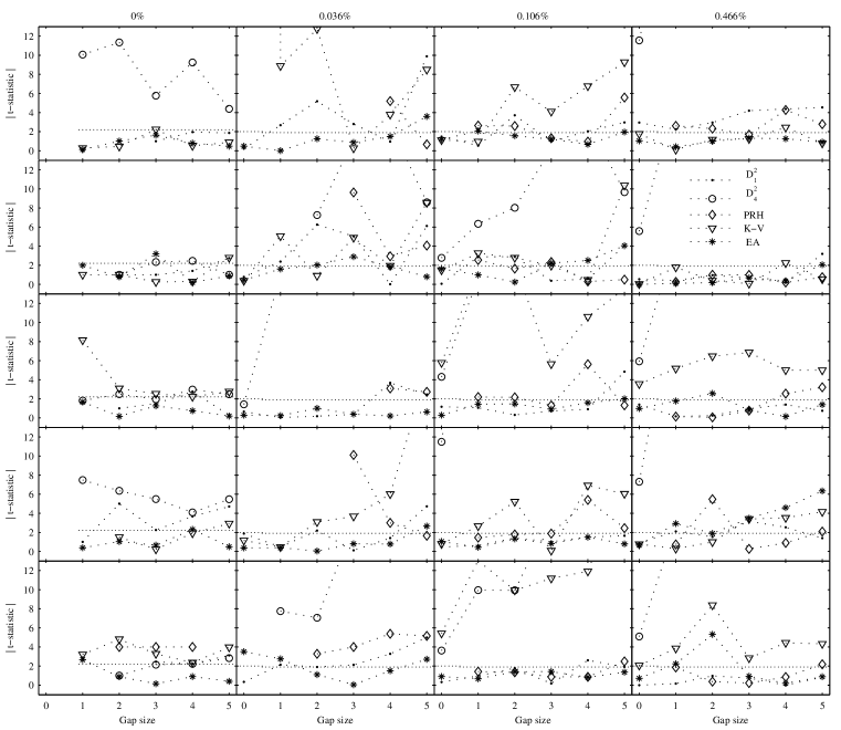
Figure 7: The $t$-test results applied to artificial Large Scale data. Each row corresponds to a different underlying function (DS-5-1,DS-5-2,…,DS-5-5), and each column corresponds to a different level of noise (0%, 0.036%, 0.106% and 0.466%). Every plot shows the results of $|{\cal T}|$ from five methods; i.e., $D_{1}^{2}$, $D_{4,2}^{2}$, PRH, K-V and EA; shaded point, circle, diamond, triangle and asterisk respectively. Note that all the plots have the same scale on the $y$-axis. See §5.2.1 for details.

Table 6: Large scale data results: $t$-test

Method	0%	0.036%	0.106%	0.466%
$D_{1}^{2}$	10	13	21	20
$D_{4,2}^{2}$	6	1	0	0
PRH	0	2	14	16
K-V	11	5	6	13
EA	22	23	24	22
see §5.2.1 for details

Like Table 6, Table 7 shows the quantity of cases where the true delay, $\Delta=5$, falls within the 95% CI. The results are also grouped by noise level. In Fig. 8, we illustrate the 95% CI for DS-5-1, i.e., one underlying function with 0% of noise only.

Table 7: Large scale data results: 95% CI

Method	0%	0.036%	0.106%	0.466%
$D_{1}^{2}$	23	14	22	20
$D_{4,2}^{2}$	12	4	0	0
PRH	0	0	0	6
K-V	19	6	6	13
EA	27	23	25	22
see §5.2.1 for details

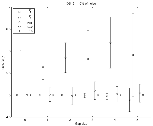
Figure 8: 95% Confidence Intervals on Large Scale Data, DS-5-1 with 0% of noise only. This plot shows the 95% CI from five methods: $D_{1}^{2}$, $D_{4,2}^{2}$, PRH, K-V and EA. The PRH intervals are not visible here because are below the bound of 4.5 days (see Table 5). We use this bound for visualisation purposes. The horizontal and dotted line is located at the true delay, $\Delta=5$.

In Fig. 9 are shown the results of MSE (14), where the estimates are grouped by level of noise as in the previous figure – Fig. 7. Here, for low levels of noise: 0% and 0.036%, the asterisk (the proposed EA) has and outstanding performance because the MSE is close to zero. The AE statistic (15) gives similar results with this grouping (not shown).

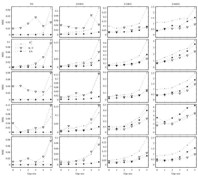
Figure 9: The use of MSE on artificial Large Scale Data. Each row corresponds to a different underlying function (DS-5-1,DS-5-2,…,DS-5-5), and each column corresponds to a different level of noise (0%, 0.036%, 0.106% and 0.466%). Every plot shows the results of MSE statistic from three methods; i.e., $D_{1}^{2}$, K-V and EA, indicated by shaded point, triangle and asterisk, respectively.

From Table 5, the best results are for $D_{1}^{2}$, K-V and EA. Since the noise is about 0.01 mag ($<0.106\%$) (standard deviation) in the observational optical data, we are interested in exploring the effects of various levels of noise. Therefore, in Table 8, we show the results of the estimates grouped by noise level, regardless of the gap size. The best results are highlighted in bold. As in Tables 6 and 7, and Figure 9, the results from EA are promising.

Table 8: Large scale data results grouped by noise level

	Noise Level
Statistic	0%	0.036%	0.106%	0.466%
Method: $D_{1}^{2}$
MSE	0.017	0.044	0.182	2.014
AE	0.060	0.147	0.321	1.121
$\hat{\mu}$	4.95	4.98	4.98	5.07
$\hat{\sigma}$	0.12	0.20	0.42	1.41
Method: K-V
MSE	0.029	0.041	0.084	1.312
AE	0.117	0.139	0.219	0.833
$\hat{\mu}$	4.93	4.94	4.93	4.96
$\hat{\sigma}$	0.11	0.13	0.21	0.83
Method: EA
MSE	1.9e-4	0.008	0.090	1.831
AE	4.7e-3	0.066	0.216	0.984
$\hat{\mu}$	4.99	4.99	4.99	5.05
$\hat{\sigma}$	0.01	0.09	0.30	1.35
$\eta$	255	12,750	12,750	12,750

Finally, we compare the performances of methods $D_{1}^{2}$, K-V and EA through paired tests on time delay estimates and MSE. As an example, in Fig. 10, we show K-V against EA with paired $t$-test. The bars represent the mean estimator $\hat{\mu}-\mu_{0}$ for each method, where $\hat{\mu}$ is the mean of time delay estimates, and $\mu_{0}$ is the true time delay. At the top of each plot appears either a circle or a plus symbol representing K-V and EA, respectively. If ${\rm MSE}_{K-V}<{\rm MSE}_{EA}$ then a circle appears, and we display the plus symbol when ${\rm MSE}_{K-V}>{\rm MSE}_{EA}$. The asterisk at the top means that the difference is significant at the level ${\cal P}<0.05$, i.e., 95% confidence level. In simple words, if the bar is large then the results are bad, because one is far from the true value $\mu_{0}=5$. Note that when the noise is low, 0%, 0.036% and 0.106%, the empty bars (EA) are small, that is, when the plus symbol (+) appears at the top. Therefore the results from EA are interesting. Moreover, note that the asterisk (*) at the top appears in some cases. The asterisk means that the comparison is significant when performing the paired $t$-test with a 95% confidence level.

In Table 9, we summarise the number of cases where ${\cal P}<0.05$, including paired sign test and paired-sample Wilcoxon signed-rank test. We also compare the results from $D_{1}^{2}$ with K-V and EA. For each comparison, the pairs are represented by $M_{1}$ (o) and $M_{2}$ ($+$). The columns corresponding to $t$-test show two quantities. The first one corresponds to the quantity of symbols “o” ($M_{1}$) with an asterisk also. The second one is the quantity of symbols “+” ($M_{2}$) with asterisks. To obtain these numbers one should imagine a figure similar to Fig. 10 for the methods involved. The columns for sign test and signed-rank test are obtained in a similar manner; rather than $t$-test in Fig. 10, were used other tests. Note again that the best results are from EA.

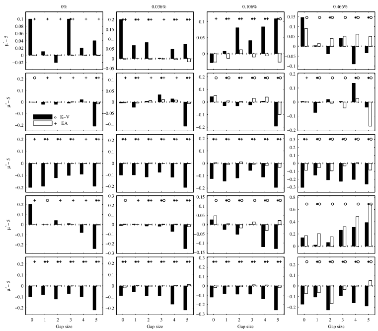
Figure 10: Paired $t$-test on Large Scale Data. The paired $t$-test is performed on time delay estimates from K-V and EA. Bars represent the estimator $\hat{\mu}-\mu_{0}$. At the top of each plot, a circle appears when ${\rm MSE}_{K-V}<{\rm MSE}_{EA}$, and the plus symbol when ${\rm MSE}_{K-V}>{\rm MSE}_{EA}$. The asterisk at top means that the p-value resulting from paired $t$-test is less than 0.05, i.e., 95% confidence level.

Table 9: Large scale data results: paired tests

		$t$-test		sign test		signed-rank test
$M_{1}$ (o)	$M_{2}$ ($+$)	$*$o	$*+$	$*$o	$*+$	$*$o	$*+$
$D_{1}^{2}$	EA	3	46	2	23	3	37
$D_{1}^{2}$	K-V	18	51	17	50	17	49
K-V	EA	28	53	25	49	29	51
see Fig. 10 and §5.2.1 for details

Now lets summarise the results found so far, Table 5 contains the results of the analysis of these data sets over all time delay estimates regardless of noise and gap size. Each row corresponds to a different statistic: 95% CI, MSE, AE, $\hat{\mu}$ and $\hat{\sigma}$. The accuracy is measured by MSE and AE, where the best results are for K-V, which is followed by EA. Since $\hat{\mu}$ and $\hat{\sigma}$ are the mean and standard deviation over all estimates, these statistics can be seen as a measurement of bias and variance of time delay estimates over all data sets. Since the true delay is $\mu_{0}=5$, the minimum bias is for $D_{1}^{2}$ ($|5.013-\mu_{0}|=0.013$); in second place is EA ($|5.015-\mu_{0}|=0.015$). The minimum variance is for K-V (0.68); in second position is EA (0.79).

However, in practice, the noise is about 0.01 mag ($<0.106\%$) for the optical data. In Tables 6 to 8, and Figs. 7, 9 and 10, the results are grouped by noise level. Tables 6 and 7 suggest that the results from EA are more statistically significant than others (see §5.2.1). Table 8 shows that the results are also better from EA, particularly when the noise is less than 0.106%. If the noise level is equal to 0.106%, depending on the statistic, the best performance is by either K-V or EA. When the noise is high (0.466%), the best results are from K-V. This can be also seen in Figs. 9 and 10.

The results from paired tests in Table 9 also suggest that the EA is capable of producing significantly superior time delay estimates, when compared to $D_{1}^{2}$ and K-V.

5.2.2 PRH Data

Now lets compare the performance of the proposed method EA with another kind of data. Here we use the artificial data generated by the PRH methodology (see §5.2 in [41] and §6 in [14]), so we compare only the PRH method against EA. In fact, we compare the performance of EA with the PRH method by fixing the PRH parameters to those values used to generate the data (the ideal scenario). The structure function (SF) to define the covariance matrix in the PRH method is used in two ways: SF is fixed to its true value (SF*) and then estimated following the PRH method (SF+).

Note that for these data there are several true time delays, $\mu_{0}$. In all cases, we use bounds of $\mu_{0}\pm 30$ days with unitary increments during the time delay analysis. The measurement error is also fixed at its true value (variance of $1\times 10^{-7}$) for all methods.

The results for the PRH method, SF* case, are in Table 10. The column $\mu_{0}$ denotes the true time delay, which is also our hypothesis in the $t$-test, whereas $\eta=100$. The following columns are the statistics used in this analysis (see section §5.2.1). The last row is the average (Avg). The results for the SF+ case and for EA are in Table 11 and Table 12 respectively. An analysis of bias ($|\mu_{0}-\hat{\mu}|$) and variance ($\hat{\sigma}$) is in Table 13.

Table 10: PRH data results: statistical analysis of the idealised method, PRH method with SF*.

$\mu_{0}$	${\cal P}$	${\cal T}$	95% CI	CI range	AE	MSE
34	1.000	0.000	33.5 - 34.4	0.92	0.44	5.28
43	0.702	0.382	42.2 - 44.1	1.87	1.54	21.96
49	0.839	2.375	49.2 - 52.0	2.81	2.36	52.32
59	0.447	1.899	58.9 - 61.1	2.21	1.78	31.96
66	0.465	0.272	65.5 - 66.5	1.02	0.71	6.55
76	0.671	2.026	76.0 - 77.5	1.55	0.95	15.67
99	0.001	2.701	99.5 - 102.3	2.86	2.79	55.39
Avg	0.374			1.89	1.51	27.02

Table 11: PRH data results: statistical analysis of PRH method with SF+.

$\mu_{0}$	${\cal P}$	${\cal T}$	95% CI	CI range	AE	MSE
34	0.000	-4.881	18.9 -27.6	8.72	22.79	593.45
43	0.210	1.260	81.8 - 48.2	6.46	13.51	266.19
49	0.315	-1.008	43.7 - 50.7	6.96	15.15	307.95
59	0.977	-0.028	54.6 - 63.1	8.51	19.66	455.20
66	0.257	-1.138	58.7 - 67.9	9.23	22.21	542.99
76	0.031	-2.188	66.7 - 75.5	8.83	20.95	513.97
99	0.407	-0.832	93.0 - 101.4	8.39	18.84	446.00
Avg	0.314			8.16	19.02	446.54

Table 12: PRH data results: statistical analysis of EA.

$\mu_{0}$	${\cal P}$	${\cal T}$	95% CI	CI range	AE	MSE
34	0.600	0.525	32.3 - 36.8	4.58	7.68	132.27
43	0.330	0.977	42.5 - 44.4	1.96	2.28	24.34
49	0.389	-0.864	46.8 - 49.8	2.94	3.99	54.69
59	0.684	0.407	57.2 - 61.9	4.35	7.28	119.00
66	0.957	-0.052	63.9 - 67.9	3.98	7.16	99.53
76	0.301	-1.039	73.0 - 76.9	3.83	6.89	93.42
99	0.830	0.214	96.7 - 101.7	4.94	8.61	153.43
Avg	0.585			3.80	6.27	96.67

Table 13: PRH data results: Bias ($|\mu_{0}-\hat{\mu}|$) versus Variance ($\hat{\sigma}$).

	PRH with SF*			PRH with SF+			EA
$\mu_{0}$	$\hat{\mu}$	$\hat{\sigma}$	Bias	$\hat{\mu}$	$\hat{\sigma}$	Bias	$\hat{\mu}$	$\hat{\sigma}$	Bias
34	34.0	2.3	0.00	23.2	21.9	10.73	34.4	11.8	0.46
43	43.1	4.7	0.18	45.0	16.2	2.05	43.7	4.8	0.79
49	50.6	7.0	1.68	47.2	17.5	1.77	48.4	7.7	0.57
59	60.0	5.5	0.07	58.9	21.4	0.06	59.9	9.7	0.96
66	66.0	2.5	0.07	63.3	23.2	2.65	65.7	9.2	0.21
76	76.7	3.8	0.79	71.1	22.2	4.87	75.1	10.2	0.86
99	100.9	7.2	1.95	97.2	21.1	1.76	99.8	12.2	0.89
Avg		4.7	0.81		20.5	3.41		9.4	0.68

Results from paired tests are in Table 14, where the p-values are shown. The best values are in bold, i.e., ${\cal P}<0.05$.

Table 14: PRH Data results: paired tests

	paired $t$-test		paired sign test		paired signed-rank test
$\mu_{0}$	SF* & EA	SF+ & EA	SF* & EA	SF+ & EA	SF* & EA	SF+ & EA
34	0.685	2.7e-5a	0.483	0.001a	0.556	4.2e-5a
43	0.364	0.476	0.057	0.089	0.004b	0.249
49	0.021a	0.567	0.012a	0.193	0.002a	0.425
59	0.919	0.673	0.012b	0.069	0.284	0.847
66	0.759	0.358	0.617	0.483	0.706	0.358
76	0.112	0.113	5e-4b	0.368	0.001b	0.145
99	0.457	0.288	0.920	0.012a	0.920	0.238
see §5.2.2 for details.
a EA with minimum MSE.
b PRH method with SF* has the minimum MSE.

Tables 10-13 show the results of the analysis applied to PRH data. Two versions of the PRH method were used: SF* and SF+ (see 5.2.2). Here, contrary to the analysis of the large scale data, the noise level and gap size are fixed (see §2). Rather, we use different short delays in the range of 30 – 100 days.

Comparing Tables 10-12, the highest significance level (${\cal P}$) on $\mu_{0}=\{34,43\}$ is for the PRH method (SF*). EA has better significance levels than the PRH method for $\mu_{0}=\{66,99\}$, even considering the idealised case. For CI range, MSE and AE statistics, SF* has the best performance on any $\mu_{0}$. But, on all statistics EA performs better than SF+. Therefore, EA is more accurate than PRH method (SF+).

In Table 13, we have $\hat{\mu}$ and $\hat{\sigma}$ as a time delay estimator and a measurement of uncertainty, respectively. Hence, the column Bias is given by $|\mu_{0}-\hat{\mu}|$. The last row has the average (Avg). Therefore, the minimum bias is for EA (on average). If we use $\hat{\sigma}$ as variance measurement, the minimum variance is for PRH method (SF*). But, EA has lower variance than SF+.

Table 14 shows that in few cases the paired difference between estimates is statistically significant (in bold). In those cases, EA is more accurate than PRH method (SF+), and in some cases EA is also more accurate than PRH method (SF*).

5.2.3 Wiener Data

Similarly, we compare the performance of EA with another kind of data (see §2). These data come from a Bayesian approach [23]. We performed an analysis as above with $\eta=225$, so the hypothesis to test is $H_{0}:\mu_{0}=35$.

The results are shown in Table 15. Since the data were generated by the Bayesian method, we aim to compare such a method with EA only.

Table 15: Wiener Data results: Statistical Analysis

		Data Set
Method	Statistic	0.1	0.2	0.4
	${\cal P}$	0.59	0.63	0.06
Bayesian method	${\cal T}$	0.52	0.48	1.87
	MSE	32.18	9.43	41.89
	AE	1.84	1.94	3.7
	$\hat{\mu}$	35.2	35.1	35.8
	$\hat{\sigma}$	5.7	3.1	6.4
	${\cal P}$	0.92	0.76	0.007
EA	${\cal T}$	0.09	0.30	2.70
	MSE	10.06	23.25	66.99
	AE	1.76	3.28	5.72
	$\hat{\mu}$	35.0	35.1	36.4
	$\hat{\sigma}$	3.1	4.8	8.0

In Table 16 are the results from paired tests between Bayesian estimation method and our EA. We highlight in bold the p-values that are less than 0.05.

Table 16: Wiener Data results: Paired Tests

	Data Set
Paired test	0.1	0.2	0.4
$t$-test	0.633	0.982	0.264
sign	0.505	0.893	0.007
signed-rank	0.827	0.766	0.005

In Table 15, the EA results are more significant for data with noise levels of 0.1 and 0.2, where ${\cal P}$ is 0.92 and 0.76 respectively. But for a noise level of 0.4, it does not perform as well. In terms of bias, EA performs better for the data with a noise level of 0.1, and ties in the case of that with 0.2 data and on the noise of 0.4 data, the performance is not good enough. Talking about variance $\hat{\sigma}$, EA is better on data set of noise 0.1 only. It needs to be emphasised though, that these data was generated by the Bayesian estimation method, so the comparison is positively biased towards the Bayesian method. However, Table 16 suggests that most of the paired differences between estimates by both methods are not statistically significant.

The poorer performance of the Bayesian method for low noise data, compared to medium noise is explained by the posterior sampler, which does not converge properly in some of the cases, giving biased estimates. This can be easily avoided when analysing any given data set, since the convergence can be assessed and the sampler re-run with different parameters. With the repeated runs performed here, the same parameters for the sampler with all of the datasets were used. In the low noise case, the convergence measurement indicates that, for a number of cases, these have not been optimal.

5.2.4 Loss Functions

Talking about loss functions, we compared the K-V and EA methods on Large Scale data (see §5.2.1). On the one hand, K-V employs the negative log-likelihood ($Q$)[14] as loss function, where the parameters $k$ and $\lambda$ are estimated via cross-validation for trial time delays in the range $0\!-\!10$. On the other hand, the fitness function of EA is the MSE_CV given by cross-validation. We also compared the K-V method with EA by using the mean squared error as the measurement of goodness of fit for K-V, rather than the negative log-likelihood. Thus, the observational error is considered constant, because the negative log likelihood fitting criterion in K-V has the form [14],

$$\ Q=\sum_{i=1}^{n}\left(\frac{(x_{A}(t_{i})-h_{A}(t_{i}))^{2}}{\sigma_{A}^{2}(t_{i})}+\frac{(x_{B}(t_{i})-M\ominus h_{B}(t_{i}))^{2}}{\sigma_{B}^{2}(t_{i})}\right).$$ (16)

For the K-V method, the negative log-likelihood cost function (16) lead to more accurate estimates.

Furthermore, we tested another fitness function on these data. Instead of MSE_CV, the fitness is given by the log-likelihood $Q$, where no cross-validation is performed, since $k$ and $\theta$ are also evolved. The results are that MSE_CV performs better than $Q$, where $Q$ is less time-consuming.

5.2.5 Evolving Weights

We also tried to evolve all the free parameters; that is, the weights $\vec{\alpha}$ in (3)-(4). This allowed us to avoid SVD in (10), which is $O(n^{3})$ (without cross-validation). However, the performance is poor because the number of parameters to evolve increases with the number of samples $n$. In fact, we tested this approach on artificial data and the performance was inferior to that of our EA. This is due to an overwhelming number of variables. Typically, using evolutionary approaches, one can well optimise in about 30-dimensional search space [49]. Perhaps a new framework can overcome this problem.

6 Conclusions

From observed optical monitoring data, we suggest 419.6 days as the best plausible value of the time delay between the two main images (A and B) of the distant lensed quasar Q0957+561.

Regarding the artificial large scale data, the results from EA are important, because its accuracy in this application is matched to the precision and low levels of noise with which the current state-of-the art optical monitoring data are being acquired for multiple-image time delay measurement [11, 33, 40, 17].

From PRH data, we conclude that EA is more accurate than PRH method (SF+), and competitive with the idealised case (SF*). Unfortunately for the PRH method, the idealised case does not exist in practice.

For the Wiener data, the conclusion is that for these data, EA outperforms Bayesian estimation method for low levels of noise (0.1 data). In other cases, depending on the statistic, EA can show better, equal or worse results. We stress that the current real optical obsrevational data are indeed characterised by low levels of observational noise. It is exactly in this context where our EA method outperforms the Bayesian estimation method.

An evolutionary algorithm has been introduced to form a novel hybridisation with our kernel method, which is an automatic method to estimate the time delay, kernels width, and SVD regularisation parameters. It is a successful application of EA driven by a model based formulation to a real-world problem. The study of the statistical significance of results on different data shows that EA is a promising approach on gravitational lensing, in astrophysics, but it can also be applied in other disciplines involving similar time series data.

7 Future Work

One of the main issues to deal with, in future extensions of this work, is speeding up our EA, which potentially can be done in several ways. First, we would seek the optimum procedure to invert (10) and its regularisation to deal with ill-conditioning (see 3). Alternative ways for model selection, rather than using cross-validation, which is $O(n^{3})$, are desirable (see in §4). The natural parallelisation of EA is another research line to follow; e.g., see [8]. To speed up the EA, fitness approximation techniques may also help with this problem [44, 34] since our fitness function is costly. Moreover, other evolutionary approaches in presence of uncertainties have not been tested [28, 2].

The time delay problem is still a huge issue in astrophysics. The next generation of large-scale monitoring projects with dedicated telescopes, LSST (http://www.lsst.org/) and PAN-STARRS (http://pan-starrs.ifa.hawaii.edu/) will produce monitoring data for thousands of potential multiply-imaged sources (as opposed to the 10 sources for which data are now available). These datasets will be available in a few years’ time, and a large effort is underway to develop algorithms that are far more sophisticated than the currently available ones that would deal with this data in an automated way, and can cope with the inevitable noise and gap features of the data. We are attempting to develop robust methods that will do this.

References

- [1] T. Anderson, S. Sclove, An Introduction to the Statistical Analysis of Data, Houghton Mifflin Company, 1978.
- [2] D. Arnold, H. Beyer, A general noise model and its effects on evolution strategy performance, IEEE Transactions on Evolutionary Computation 10 (4) (2006) 380–391.
- [3] D. A. Berry, B. W. Lindgren, Statistical Theory and Methods, Brooks/Cole Publishing Company, 1998.
- [4] J. Biethahn, V. Nissen, Evolutionary Algorithms in Management Applications, Springer-Verlag, Berlin, 1995.
- [5] E. Bonilla-Huerta, B. Duval, J.-K. Hao, A hybrid ga/svm approach for gene selection and classification of microarray data, in: F. R. et al. (ed.), Applications of Evolutionary Computing, EvoWorkshops 2006, LNCS 3907, Springer-Verlag, 2006.
- [6] W. Bridewell, P. Langley, S. Racunas, S. Borrett, Learning process models with missing data, in: Machine Learning: ECML 2006, Lecture Notes in Artificial Intelligence (LNAI 4212), Springer-Verlag, 2006.
- [7] I. Burud, P. Magain, S. Sohy, J. Hjorth, A novel approach for extracting time-delays from lightcurves of lensed quasar images, Astronomy and Astrophysics 380 (2) (2001) 805–810.
- [8] E. Cant -Paz, D. Goldberg, Efficient parallel genetic algorithms: theory and practice, Computer Methods in Applied Mechanics and Engineering 186 (1) (2000) 221–238.
- [9] A. J. Chipperfield, P. J. Fleming, C. M. Fonseca, Genetic algorithm tools for control systems engineering, in: Proc.1st Int. Conf. Adaptive Computing in Engineering Design and Control, Plymouth Engineering Design Centre,UK, 1994, http://www.shef.ac.uk/acse/research/ecrg/getgat.html.
- [10] A. J. Chipperfield, P. J. Fleming, H. Pohlheim, C. M. Fonseca, Genetic Algorithm Toolbox for use with MATLAB, Automatic Control and Systems Engenieering, University of Sheffield, 1st ed., http://www.shef.ac.uk/acse/research/ecrg/getgat.html (1996).
- [11] W. Colley, R. Schild, C. Abajas, D. Alcalde, Z. Aslan, I. Bikmaev, V. Chavushyan, L. Chinarro, J. Cournoyer, R. Crowe, V. Dudinov, A. Evans, Y. Jeon, L. Goicoechea, O. Golbasi, I. Khamitov, K. Kjernsmo, H. Lee, J. Lee, K. Lee, M. Lee, O. Lopez-Cruz, E. Mediavilla, A. Moffat, R.Mujica, A. Ullan, J. Munoz, A. Oscoz, M. Park, N. Purves, O. Saanum, N. Sakhibullin, M. Serra-Ricart, I. Sinelnikov, R. Stabell, A. Stockton, J. Teuber, R. Thompson, H. Woo, A. Zheleznyak, Around-the-clock observations of the Q0957+561 A,B gravitationally lensed quasar. II. Results for the second observing season, Astronomy and Astrophysics 587 (1) (2003) 71–79.
- [12] R. Cook, D. McLeish (eds.), Workshop on Missing Data Problems, Fields Institute, Toronto, Canada, 2004, http://www.fields.utoronto.ca/programs/scientific/04-05/missing-data/ (2004).
- [13] G. Cowan, Statistical Data Analysis, Oxford University Press, 1998.
- [14] J. Cuevas-Tello, P. Tiňo, S. Raychaudhury, How accurate are the time delay estimates in gravitational lensing?, Astronomy and Astrophysics 454 (2006) 695–706.
- [15] J. Cuevas-Tello, P. Tiňo, S. Raychaudhury, A kernel-based approach to estimating phase shifts between irregularly sampled time series: an application to gravitational lenses, in: Machine Learning: ECML 2006, Lecture Notes in Artificial Intelligence (LNAI 4212), Springer-Verlag, 2006.
- [16] E. J. Dudewicz, S. N. Mishra, Modern Mathematical Statistics, John Wiley and Sons, 1988.
- [17] A. Eigenbrod, F. Courbin, C. Vuissoz, G. Meylan, P. Saha, S. Dye, COSMOGRAIL: The COSmological MOnitoring of GRAvItational Lenses. I. How to sample the light curves of gravitationally lensed quasars to measure accurate time delays, Astronomy and Astrophysics 436 (2005) 25–35.
- [18] J. Fohlmeister, C. S. Kochanek, E. E. Falco, C. W. Morgan, J. Wambsganss, The Rewards of Patience: An 822 Day Time Delay in the Gravitational Lens SDSS J1004+4112, Astrophysical Journal 676 (2008) 761–766.
- [19] O. Giel, P. Lehre, On the effect of populations in evolutionary multi-objective optimization, in: M. K. et al. (ed.), Genetic and Evolutionary Computation Conference (GECCO), vol. 1, ACM Press, 2006.
- [20] D. Goldberg, Genetic Algorithms in Search, Optimization, and Machine Learning, Addison-Wesley, 1989.
- [21] G. Golub, C. V. Loan, Matrix Computations, 2nd ed., The Johns Hopkins University Press, 1989.
- [22] D. Haarsma, J. Hewitt, J. Lehar, B. Burke, The radio wavelength time delay of gravitational lens 0957+561, Astrophysical Journal 510 (1) (1999) 64–70.
- [23] M. Harva, S. Raychaudhury, Bayesian estimation of time delays between unevenly sampled signals, in: IEEE International Workshop on Machine Learning for Signal Processing, IEEE, 2006.
- [24] M. Harva, S. Raychaudhury, Bayesian estimation of time delays between unevenly sampled signals, Neurocomputing 72 (1-3) (2008) 32–38.
- [25] T. Hastie, R. Tibshirani, J. Friedman, The Elements of Statistical Learning: Data Mining, Inference, and Prediction, Springer, 2001.
- [26] T. Howley, M. G. Madden, The genetic kernel support vector machine: Description and evaluation, Artificial Intelligence Review 24 (3) (2005) 379–395.
- [27] N. Inada, M. Oguri, R. H. Becker, M.-S. Shin, G. T. Richards, J. F. Hennawi, R. L. White, B. Pindor, M. A. Strauss, C. S. Kochanek, D. E. Johnston, M. D. Gregg, I. Kayo, D. Eisenstein, P. B. Hall, F. J. Castander, A. Clocchiatti, S. F. Anderson, D. P. Schneider, D. G. York, R. Lupton, K. Chiu, Y. Kawano, R. Scranton, J. A. Frieman, C. R. Keeton, T. Morokuma, H.-W. Rix, E. L. Turner, S. Burles, R. J. Brunner, E. S. Sheldon, N. A. Bahcall, F. Masataka, The Sloan Digital Sky Survey Quasar Lens Search. II. Statistical Lens Sample from the Third Data Release, Astronomical Journal 135 (2008) 496–511.
- [28] Y. Jin, J. Branke, Evolutionary optimization in uncertain enviroments – a survey, IEEE Transactions on Evolutionary Computation 9 (3) (2005) 303–317.
- [29] C. Kochanek, P. Schechter, The Hubble constant from gravitational lens time delays, in: W. L. Freedman (ed.), Measuring and Modeling the Universe, from the Carnegie Observatories Centennial Symposia, vol. 2, Cambridge University Press, 2004.
- [30] T. Kundic, E. Turner, W. Colley, J. Gott-III, J. Rhoads, Y. Wang, L. bergeron, K. Gloria, D. Long, S. Malhorta, J. Wambsganss, A robust determination of the time delay in 0957+561A,B and a measurement of the global value of Hubble’s constant, Astrophysical Journal 482 (1) (1997) 75–82.
- [31] T. Mitchell, Machine Learning, Computer Science, McGraw-Hill, 1997.
- [32] M. Oguri, Gravitational Lens Time Delays: A Statistical Assessment of Lens Model Dependences and Implications for the Global Hubble Constant, Astrophysical Journal 660 (2007) 1–15.
- [33] J. Ovaldsen, J. Teuber, R. Schild, R. Stabell, New aperture photometry of QSO 0957+561; application to time delay and microlensing, Astronomy and Astrophysics 402 (3) (2003) 891–904.
- [34] I. Paenke, J. Branke, Y. Jin, Efficient search for robust solutions by means of evolutionary algorithms and fitness approximation, IEEE Transactions on Evolutionary Computation 10 (4) (2006) 405–420.
- [35] J. Pelt, J. Hjorth, S. Refsdal, R. Schild, R. Stabell, Estimation of multiple time delays in complex gravitational lens systems, Astronomy and Astrophysics 337 (3) (1998) 681–684.
- [36] J. Pelt, R. Kayser, S. Refsdal, T. Schramm, Time delay controversy on QSO 0957+561 not yet decided, Astronomy and Astrophysics 286 (1) (1994) 775–785.
- [37] J. Pelt, R. Kayser, S. Refsdal, T. Schramm, The light curve and the time delay of QSO 0957+561, Astronomy and Astrophysics 305 (1) (1996) 97–106.
- [38] T. Phienthrakul, B. Kijsirikul, Evolutionary strategies for multi-scale radial basis function kernels in support vector machines, in: H.-G. B. et al. (ed.), Genetic and Evolutionary Computation Conference (GECCO), vol. 1, 2005.
- [39] F. Pijpers, The determination of time delays as an inverse problem - the case of the double quasar 0957+561, Monthly Notices of the Royal Astronomical Society 289 (4) (1997) 933–944.
- [40] B. Pindor, Discovering Gravitational Lenses through Measurements of Their Time Delays, Astrophysical Journal 626 (2005) 649–656.
- [41] W. Press, G. Rybicki, J. Hewitt, The time delay of gravitational lens 0957+561, I. Methodology and analysis of optical photometric Data, Astrophysical Journal 385 (1) (1992) 404–415.
- [42] W. Press, S. Teukolsky, W. Vetterling, B. Flannery, Numerical Recipes in C++: The Art of Scientific Computing, 2nd ed., Cambridge University Press, 2002.
- [43] S. Refsdal, On the possibility of determining the distances and masses of stars from the gravitational lens effect, Monthly Notices of the Royal Astronomical Society 134 (1966) 315–319.
- [44] R. Regis, C. Shoemaker, Local function approximation in evolutionary algorithms for the optimization of costly functions, IEEE Transactions on Evolutionary Computation 8 (5) (2004) 490–505.
- [45] J. E. Rowe, D. Hidovic, An Evolution Strategy using a continuous version of the Gray-code neighbourhood distribution, in: K. D. et al. (ed.), Genetic and Evolutionary Computation Conference (GECCO), vol. 1, Springer-Verlag, 2004.
- [46] P. Saha, Gravitational Lensing, in: P. Murdin (ed.), Encyclopedia of Astronomy and Astrophysics, Nature Publishing, London, 2001.
- [47] J. Shawe-Taylor, N. Cristianini, Kernel Methods for Pattern Analysis, Cambridge University Press, 2004.
- [48] W. M. Spears, Evolutionary Algorithms: The role of Mutation and Recombination, Natural computing, Springer-Verlag, 2000.
- [49] Z. Tu, Y. Lu, A Robust Stochastic genetic Algorithm (StGA) for Global Numerical Optimization , IEEE Transactions on Evolutionary Computation 8 (2004) 456–470.
- [50] C. Vuissoz, F. Courbin, D. Sluse, G. Meylan, V. Chantry, E. Eulaers, C. Morgan, M. E. Eyler, C. S. Kochanek, J. Coles, P. Saha, P. Magain, E. E. Falco, COSMOGRAIL: the COSmological MOnitoring of GRAvItational Lenses. VII. Time delays and the Hubble constant from WFI J2033-4723, Astronomy and Astrophysics 488 (2008) 481–490.
- [51] D. Walsh, R. F. Carswell, R. J. Weymann, 0957 + 561 A, B - Twin quasistellar objects or gravitational lens, Nature 279 (1979) 381–384.
- [52] X. Yao, Y. Liu, G. Lin, Evolutionary programming made faster, IEEE Transactions on Evolutionary Computation 3 (2) (1999) 82–102.