Bit-Interleaved Coded Multiple Beamforming with Constellation Precoding

Abstract

In this paper, we present the diversity order analysis of bit-interleaved coded multiple beamforming (BICMB) combined with the constellation precoding scheme. Multiple beamforming is realized by singular value decomposition of the channel matrix which is assumed to be perfectly known to the transmitter as well as the receiver. Previously, BICMB is known to have a diversity order bound related with the product of the code rate and the number of parallel subchannels, losing the full diversity order in some cases. In this paper, we show that BICMB combined with the constellation precoder and maximum likelihood detection achieves the full diversity order. We also provide simulation results that match the analysis.

I Introduction

When the perfect channel state information is available at the transmitter to achieve spatial multiplexing and thereby increase the data rate, or to enhance the performance of a multi-input multi-output (MIMO) system, beamforming can be employed [1]. The beamforming vectors are designed in [2], [3] for various design criteria, and can be obtained by singular value decomposition (SVD), leading to a channel-diagonalizing structure optimum in minimizing the average bit error rate (BER) [3].

It is known that an SVD subchannel with larger singular value provides larger diversity gain. During the simultaneous parallel transmission of the symbols on the diagonalized subchannels, the performance is dominated by the subchannel with the smallest singular value, resulting in losing the full diversity order [4], [5]. To overcome the degradation of the diversity order of multiple beamforming, bit-interleaved coded multiple beamforming (BICMB) was proposed [6], [7]. This scheme interleaves the codewords through the multiple subchannels with different diversity orders, resulting in better diversity order. BICMB can achieve the full diversity order offered by the channel as long as the code rate $R_{c}$ and the number of subchannels used $S$ satisfy the condition $R_{c}S\leq 1$ [8].

We showed in [9] and [10] that constellation precoded multiple beamforming, which converts a symbol into a precoded symbol and distributes the precoded symbol over the subchannels, can compensate for the diversity loss caused by the uncoded multiple beamforming. In this paper, by calculating pairwise error probability (PEP), we present the diversity analysis of Bit-Interleaved Coded Multiple Beamforming with Constellation Precoding (BICMB-CP), which adds the constellation precoding stage to BICMB. We show that adding the constellation precoder to the BICMB system which does not satisfy the full diversity condition guarantees the full diversity order when the subchannels to transmit the precoded symbols are properly chosen. Simulation results are shown to prove the analysis.

The rest of this paper is organized as follows. The description of BICMB-CP is given in Section II. Section III presents the diversity analysis through the calculation of the upper bound to PEP. Simulation results supporting the analysis are shown in Section IV. Finally, we end the paper with our conclusion in Section V.

Notation: Bold lower (upper) case letters denote vectors (matrices). $\textrm{diag}[\mathbf{B}_{1},\cdots,\mathbf{B}_{P}]$ stands for a block diagonal matrix with matrices $\mathbf{B}_{1},\cdots,\mathbf{B}_{P}$, and $\textrm{diag}[b_{1},\cdots,b_{P}]$ is a diagonal matrix with diagonal entries $b_{1},\cdots,b_{P}$. The superscripts $(\cdot)^{H}$, $(\cdot)^{T}$, $(\cdot)^{*}$, $\bar{(\cdot)}$ stand for conjugate transpose, transpose, complex conjugate, binary complement, respectively, and $\forall$ denotes for-all. $\mathbb{R}^{+}$ and $\mathbb{C}$ stand for the set of positive real numbers and the complex numbers, repectively. $d_{min}$ is the minimum Euclidean distance between two points in the constellation. $N$ and $M$ stand for the number of transmit and receive antennas.

II BICMB with Constellation Precoding

Fig. 1 represents the structure of BICMB with constellation precoding. First, the code rate $R_{c}=k_{c}/n_{c}$ convolutional encoder, possibly combined with a perforation matrix for a high rate punctured code, generates the codeword $\mathbf{c}$ from the information bits. Then, the spatial interleaver distributes the coded bits into $S\leq\min(N,M)$ streams, each of which is interleaved by an independent bit-wise interleaver $\pi$. The interleaved bits are mapped by Gray encoding onto the symbol sequence $\mathbf{X}=[\mathbf{x}_{1}\,\cdots\,\mathbf{x}_{K}]$, where $\mathbf{x}_{k}$ is an $S\times 1$ symbol vector at the $k^{th}$ time instant. In this model, we assume that each stream employs the same modulation scheme. Each entry in the symbol vector belongs to a signal set $\chi\subset\mathbb{C}$ of size $|\chi|=2^{m}$, such as $2^{m}$-QAM, where $m$ is the number of input bits to the Gray encoder.

Figure 1: Structure of Bit-Interleaved Coded Multiple Beamforming with Constellation Precoding.

The symbol vector $\mathbf{x}_{k}$ is multiplied by the $S\times S$ precoder $\boldsymbol{\Theta}$, which is defined as

$$\mathbf{\Theta}=\left[\begin{array}[]{cc}\mathbf{\tilde{\Theta}}&\mathbf{0}\\ \mathbf{0}&\mathbf{I}_{S-P}\end{array}\right]$$ (3)

where $\mathbf{\tilde{\Theta}}$ is the $P\times P$ unitary constellation precoding matrix that precodes the first $P$ modulated entries of the vector $\mathbf{x}_{k}$. When all of the $S$ modulated entries are precoded ($P=S$), we call the resulting system Bit-Interleaved Coded Multiple Beamforming with Full Precoding (BICMB-FP), otherwise, we call it Bit-Interleaved Coded Multiple Beamforming with Partial Precoding (BICMB-PP). The symbol generated by $\boldsymbol{\Theta}$ is multiplied by $\mathbf{T}$ which is an $S\times S$ permutation matrix to define the mapping of the precoded and non-precoded symbols onto the predefined subchannels. Let us define $\mathbf{b}_{p}=\left[b_{p}(1)\,\cdots\,b_{p}(P)\right]$ as a vector whose element $b_{p}(u)$ is the subchannel on which the precoded symbols are transmitted, and ordered increasingly such that $b_{p}(u)<b_{p}(v)$ for $u<v$. In the same way, $\mathbf{b}_{n}=\left[b_{n}(1)\,\cdots\,b_{n}(S-P)\right]$ is defined as an increasingly ordered vector whose element $b_{n}(u)$ is the subchannel which carries the non-precoded symbols.

The MIMO channel $\mathbf{H}\in\mathbb{C}^{M\times N}$ is assumed to be quasi-static, Rayleigh, and flat fading, and perfectly known to both the transmitter and the receiver. In this channel model, we consider that the channel coefficients remain constant for the $K$ symbol duration. The beamforming vectors are determined by the SVD of the MIMO channel, i.e., $\mathbf{H}=\mathbf{U\Lambda V}^{H}$ where $\mathbf{U}$ and $\mathbf{V}$ are unitary matrices, and $\mathbf{\Lambda}$ is a diagonal matrix whose $s^{th}$ diagonal element, $\lambda_{s}\in\mathbb{R}^{+}$, is a singular value of $\mathbf{H}$ in decreasing order. When $S$ symbols are transmitted at the same time, then the first $S$ vectors of $\mathbf{U}$ and $\mathbf{V}$ are chosen to be used as beamforming matrices at the receiver and the transmitter, respectively. $\mathbf{\tilde{U}}$ and $\mathbf{\tilde{V}}$ in Fig. 1 denote the first $S$ column vectors of $\mathbf{U}$ and $\mathbf{V}$.

The spatial interleaver arranges the symbol vector $\mathbf{x}_{k}$ as $\mathbf{x}_{k}=[\mathbf{x}_{k,\mathbf{b}_{p}}^{T}\,\vdots\,\mathbf{x}_{k,\mathbf{b}_{n}}^{T}]^{T}=[x_{k,b_{p}(1)}\,\cdots\,x_{k,b_{p}(P)}\,\vdots$ $\,x_{k,b_{n}(1)}\,\cdots\,x_{k,b_{n}(S-P)}]^{T}$ where $\mathbf{x}_{k,\mathbf{b}_{p}}$ and $\mathbf{x}_{k,\mathbf{b}_{n}}$ are the modulated entries to be transmitted on the subchannels specified in $\mathbf{b}_{p}$ and $\mathbf{b}_{n}$, respectively. The $S\times 1$ detected symbol vector $\mathbf{r}_{k}=[(\mathbf{r}_{k}^{p})^{T}\,\vdots\,(\mathbf{r}_{k}^{n})^{T}]^{T}=[r_{k,1}\,\cdots\,r_{k,P}\,\vdots\,r_{k,P+1}\,\cdots\,r_{k,S}]^{T}$ at the $k^{th}$ time instant is

$$\mathbf{r}_{k}=\boldsymbol{\Gamma}\mathbf{\Theta x}_{k}+\mathbf{n}_{k}$$ (4)

where $\boldsymbol{\Gamma}$ is a block diagonal matrix, $\boldsymbol{\Gamma}=\textrm{diag}[\boldsymbol{\Gamma}_{p},\boldsymbol{\Gamma}_{n}]$ with diagonal matrices defined as $\boldsymbol{\Gamma}_{p}=\textrm{diag}[\lambda_{b_{p}(1)},$ $\,\cdots,\,\lambda_{b_{p}(P)}]$, $\boldsymbol{\Gamma}_{n}=\textrm{diag}[\lambda_{b_{n}(1)},\,\cdots,\,\lambda_{b_{n}(S-P)}]$, and $\mathbf{n}_{k}=[(\mathbf{n}_{k}^{p})^{T}\,\vdots\,(\mathbf{n}_{k}^{n})^{T}]^{T}=[r_{n,1}\,\cdots\,r_{n,P}\,\vdots\,r_{n,P+1}\,\cdots\,r_{n,S}]^{T}$ is an additive white Gaussian noise vector with zero mean and variance $N_{0}=N/SNR$. $\mathbf{H}$ is complex Gaussian with zero mean and unit variance, and to make the received signal-to-noise ratio $SNR$, the total transmitted power is scaled as $N$. The input-output relation in (4) is decomposed into two equations as

$$\begin{split}\mathbf{r}_{k}^{p}=\boldsymbol{\Gamma}_{p}\boldsymbol{\tilde{\Theta}}\mathbf{x}_{k,\mathbf{b}_{p}}+\mathbf{n}_{k}^{p}\\ \mathbf{r}_{k}^{n}=\boldsymbol{\Gamma}_{n}\mathbf{x}_{k,\mathbf{b}_{n}}+\mathbf{n}_{k}^{n}.\end{split}$$ (5)

The location of the coded bit $c_{k^{\prime}}$ within the symbol sequence $\mathbf{X}$ is known as $k^{\prime}\rightarrow(k,l,i)$, where $k$, $l$, and $i$ are the time instant in $\mathbf{X}$, the symbol position in $\mathbf{x}_{k}$, and the bit position on the symbol $x_{k,l}$, respectively. Let $\chi_{b}^{i}$ denote a subset of $\chi$ whose labels have $b\in\{0,1\}$ in the $i^{th}$ bit position. By using the location information and the input-output relation in (4), the receiver calculates the maximum likelihood (ML) bit metrics for the coded bit $c_{k^{\prime}}$ as

$$\gamma^{l,i}(\mathbf{r}_{k},c_{k^{\prime}})=\min_{\mathbf{x}\in\xi_{c_{k^{\prime}}}^{l,i}}\|\mathbf{r}_{k}-\boldsymbol{\Gamma}\boldsymbol{\Theta}\mathbf{x}\|^{2}$$ (6)

where $\xi_{c_{k^{\prime}}}^{l,i}$ is a subset of $\chi^{S}$, defined as

$$\xi_{b}^{l,i}=\{\mathbf{x}=[x_{1}\,\cdots\,x_{S}]^{T}:x_{s|s=l}\in\chi_{b}^{i},\textrm{ and }x_{s|s\neq l}\in\chi\}.$$

In particular, the bit metrics, equivalent to (6) for partial precoding, are represented as

$$\gamma^{l,i}(\mathbf{r}_{k},c_{k^{\prime}})=\left\{\begin{array}[]{ll}\min\limits_{\mathbf{x}\in\psi_{c_{k^{\prime}}}^{l,i}}\|\mathbf{r}_{k}^{p}-\boldsymbol{\Gamma}_{p}\boldsymbol{\tilde{\Theta}}\mathbf{x}\|^{2},&\textrm{ if $1\leq l\leq P$}\\ \min\limits_{x\in\chi_{c_{k^{\prime}}}^{i}}|r_{k,l}-\lambda_{\hat{l}}x|^{2},&\textrm{ if $P+1\leq l\leq S$}\end{array}\right.$$ (9)

where $\psi_{b}^{l,i}$ is a set which is mapped from the set $\xi_{b}^{l,i}$ by a surjective function $f(\mathbf{x})$, for $\mathbf{x}=[x_{1}\,\cdots\,x_{S}]^{T}$, defined as

$$f\left(\mathbf{x}\right)=[x_{1}\,\cdots\,x_{P}]^{T},$$

and $\hat{l}$ is an entry in $\mathbf{b}_{n}$, corresponding to the subchannel mapped by $\mathbf{T}$. Finally, the ML decoder makes decisions according to the rule

$$\mathbf{\hat{c}}=\arg\min_{\mathbf{\tilde{c}}}\sum_{k^{\prime}}\gamma^{l,i}(\mathbf{r}_{k},\tilde{c}_{k^{\prime}}).$$ (10)

III Diversity Analysis

Since BER in BICMB is bounded by the union of the PEP corresponding to each error event [6], the calculation of each PEP is needed. In particular, the overall diversity order is dominated by the pairwise errors which have the smallest exponent of signal-to-noise ratio in PEP representation. In this section, we calculate the upper bound to each PEP corresponding to the pairwise errors.

III-A BICMB with Full Precoding

Based on the bit metrics in (6), the instantaneous PEP between the transmitted codeword $\mathbf{c}$ and the decoded codeword $\mathbf{\hat{c}}$ is calculated as

$$\textrm{Pr}\left(\mathbf{c}\rightarrow\mathbf{\hat{c}}|\mathbf{H}\right)=\textrm{Pr}\left(\sum_{k^{\prime}}\min_{\mathbf{x}\in\xi_{c_{k^{\prime}}}^{l,i}}\|\mathbf{r}_{k}-\boldsymbol{\Gamma}\boldsymbol{\Theta}\mathbf{x}\|^{2}\geq\right.\left.\sum_{k^{\prime}}\min_{\mathbf{x}\in\xi_{\hat{c}_{k^{\prime}}}^{l,i}}\|\mathbf{r}_{k}-\boldsymbol{\Gamma}\boldsymbol{\Theta}\mathbf{x}\|^{2}\right)$$ (11)

where $c_{k^{\prime}}$ and $\hat{c}_{k^{\prime}}$ is the coded bit of $\mathbf{c}$ and $\mathbf{\hat{c}}$, respectively. We define $d_{H}$ as the Hamming distance between $\mathbf{c}$ and $\mathbf{\hat{c}}$. It is assumed that the $d_{H}$ coded bits are interleaved such that they are placed in distinct symbols. In addition, we know that the bit metrics corresponding to the same coded bits between the pairwise errors are the same. Based on the assumption and the knowledge, (11) is re-written as

$$\textrm{Pr}\left(\mathbf{c}\rightarrow\mathbf{\hat{c}}|\mathbf{H}\right)=\textrm{Pr}\left(\sum_{k,d_{H}}\min_{\mathbf{x}\in\xi_{c_{k^{\prime}}}^{l,i}}\|\mathbf{r}_{k}-\boldsymbol{\Gamma}\boldsymbol{\Theta}\mathbf{x}\|^{2}\geq\right.\left.\sum_{k,d_{H}}\min_{\mathbf{x}\in\xi_{\hat{c}_{k^{\prime}}}^{l,i}}\|\mathbf{r}_{k}-\boldsymbol{\Gamma}\boldsymbol{\Theta}\mathbf{x}\|^{2}\right)$$ (12)

where $\sum_{k,d_{H}}$ stands for the summation of the $d_{H}$ values that correspond to the different coded bits between the codewords.

Let us define $\mathbf{\tilde{x}}_{k}$ and $\mathbf{\hat{x}}_{k}$ as

$$\begin{split}\mathbf{\tilde{x}}_{k}=\arg\min_{\mathbf{x}\in\xi_{c_{k^{\prime}}}^{l,i}}\|\mathbf{r}_{k}-\boldsymbol{\Gamma}\boldsymbol{\Theta}\mathbf{x}\|^{2}\\ \mathbf{\hat{x}}_{k}=\arg\min_{\mathbf{x}\in\xi_{\bar{c}_{k^{\prime}}}^{l,i}}\|\mathbf{r}_{k}-\boldsymbol{\Gamma}\boldsymbol{\Theta}\mathbf{x}\|^{2}\end{split}$$ (13)

where $\bar{c}_{k^{\prime}}$ is the complement of $c_{k^{\prime}}$ in binary codes. It is easily found that $\mathbf{\tilde{x}}_{k}$ is different from $\mathbf{\hat{x}}_{k}$ since the sets that the $l^{th}$ symbols belong to are disjoint, as can be seen from the definition of $\xi_{c_{k^{\prime}}}^{l,i}$. In the same manner, we see that $\mathbf{x}_{k}$ is different from $\mathbf{\hat{x}}_{k}$. With $\mathbf{\tilde{x}}_{k}$ and $\mathbf{\hat{x}}_{k}$, we get the following expression from (12) as

$$\textrm{Pr}\left(\mathbf{c}\rightarrow\mathbf{\hat{c}}|\mathbf{H}\right)=\textrm{Pr}\left(\sum_{k,d_{H}}\|\mathbf{r}_{k}-\boldsymbol{\Gamma}\boldsymbol{\Theta}\mathbf{\tilde{x}}_{k}\|^{2}\geq\right.\left.\sum_{k,d_{H}}\|\mathbf{r}_{k}-\boldsymbol{\Gamma}\boldsymbol{\Theta}\mathbf{\hat{x}}_{k}\|^{2}\right).$$ (14)

Based on the fact that $\|\mathbf{r}_{k}-\boldsymbol{\Gamma}\boldsymbol{\Theta}\mathbf{x}_{k}\|^{2}\geq\|\mathbf{r}_{k}-\boldsymbol{\Gamma}\boldsymbol{\Theta}\mathbf{\tilde{x}}_{k}\|^{2}$ and the relation in (4), equation (14) is upper-bounded by

$$\textrm{Pr}(\mathbf{c}\rightarrow\mathbf{\hat{c}}|\mathbf{H})\leq\textrm{Pr}\left(\beta\geq\sum_{k,d_{H}}\|\boldsymbol{\Gamma}\boldsymbol{\Theta}(\mathbf{x}_{k}-\mathbf{\hat{x}}_{k})\|^{2}\right)$$ (15)

where

$$\beta=-\sum_{k,d_{H}}(\mathbf{x}_{k}-\mathbf{\hat{x}}_{k})^{H}\boldsymbol{\Theta}^{H}\boldsymbol{\Gamma}\mathbf{n}_{k}+\mathbf{n}_{k}^{H}\boldsymbol{\Gamma}\boldsymbol{\Theta}(\mathbf{x}_{k}-\mathbf{\hat{x}}_{k}).$$

Since $\beta$ is a zero mean Gaussian random variable with variance $2N_{0}\sum_{k,d_{H}}\|\boldsymbol{\Gamma}\boldsymbol{\Theta}(\mathbf{x}_{k}-\mathbf{\hat{x}}_{k})\|^{2}$, (15) is replaced by the $Q$ function as

$$\textrm{Pr}(\mathbf{c}\rightarrow\mathbf{\hat{c}}|\mathbf{H})\leq Q\left(\sqrt{\frac{\sum\limits_{k,d_{H}}\|\boldsymbol{\Gamma}\boldsymbol{\Theta}(\mathbf{x}_{k}-\mathbf{\hat{x}}_{k})\|^{2}}{2N_{0}}}\right).$$ (16)

The numerator in (16) is rewritten as

$$\sum\limits_{k,d_{H}}\|\boldsymbol{\Gamma}\boldsymbol{\Theta}(\mathbf{x}_{k}-\mathbf{\hat{x}}_{k})\|^{2}=\sum\limits_{k,d_{H}}\sum\limits_{s=1}^{S}\lambda_{s}^{2}|d_{k,s}|^{2}=\sum\limits_{s=1}^{S}\lambda_{s}^{2}\sum\limits_{k,d_{H}}|d_{k,s}|^{2}$$ (17)

where $\mathbf{d}_{k}=[d_{k,1}\cdots d_{k,S}]^{T}=\boldsymbol{\Theta}(\mathbf{x}_{k}-\mathbf{\hat{x}}_{k})$. Using an upper bound to the $Q$ function, we calculate the average PEP as

$$\textrm{Pr}(\mathbf{c}\rightarrow\mathbf{\hat{c}})\leq E\left[\exp\left(-\frac{\sum\limits_{s=1}^{S}\lambda_{s}^{2}\sum\limits_{k,d_{H}}|d_{k,s}|^{2}}{4N_{0}}\right)\right].$$ (18)

In [8], we have shown that equations with such form as (18) have a closed form expression of an upper bound. We provide a formal description below.

Theorem 1

Consider the largest $S\leq\min(N,M)$ eigenvalues $\mu_{s}$ of the uncorrelated central $M\times N$ Wishart matrix that are sorted in decreasing order, and a weight vector $\boldsymbol{\phi}=[\phi_{1}\,\cdots\,\phi_{S}]^{T}$ with non-negative real elements. In the high signal-to-noise ratio regime, an upper bound for the expression $E[\exp(-\gamma\sum_{s=1}^{S}\phi_{s}\mu_{s})]$ which is used in the diversity analysis of a number of MIMO systems is

$$E\left[\exp\left(-\gamma\sum\limits_{s=1}^{S}\phi_{s}\mu_{s}\right)\right]\leq\zeta\left(\phi_{min}\gamma\right)^{-(N-\delta+1)(M-\delta+1)}$$

where $\gamma$ is signal-to-noise ratio, $\zeta$ is a constant, $\phi_{min}=\min\{\phi_{1},\,\cdots,\,\phi_{S}\}$, and $\delta$ is the index to the first non-zero element in the weight vector.

Proof:

See [8]. ∎

By calculating the weight vector whose $s^{th}$ element is $\sum_{k,d_{H}}|d_{k,s}|^{2}$, we evaluate the diversity order of a given system. In particular, if the constellation precoder is designed such that

$$|d_{k,1}|^{2}=|\boldsymbol{\theta}_{1}^{T}(\mathbf{x}_{k}-\mathbf{\hat{x}_{k}})|^{2}>0,\forall(\mathbf{x}_{k},\mathbf{\hat{x}}_{k})$$ (19)

where $\boldsymbol{\theta}_{1}^{T}$ is the first row vector of the unitary precoding matrix $\boldsymbol{\Theta}$, we see that $\sum_{k,d_{H}}|d_{k,1}|^{2}>0$, resulting in the full diversity order of $NM$. Therefore, (19) is a sufficient condition for the full diversity order of BICMB-FP.

III-B BICMB with Partial Precoding

The bit metrics in (9) lead to the PEP calculation as

$$\textrm{Pr}\left(\mathbf{c}\rightarrow\mathbf{\hat{c}}|\mathbf{H}\right)=\textrm{Pr}\left(\tau_{1}\geq\tau_{2}\right)$$ (20)

where

$$\tau_{1} =\sum_{k,d_{H,p}}\min_{\mathbf{x}\in\psi_{c_{k^{\prime}}}^{l,i}}\|\mathbf{r}_{k}^{p}-\boldsymbol{\Gamma}_{p}\boldsymbol{\tilde{\Theta}}\mathbf{x}\|^{2}+\sum_{k,d_{H,n}}\min_{x\in\chi_{c_{k^{\prime}}}^{l,i}}|r_{k,l}-\lambda_{\hat{l}}x|^{2}$$

$$\tau_{2} =\sum_{k,d_{H,p}}\min_{\mathbf{x}\in\psi_{\bar{c}_{k^{\prime}}}^{l,i}}\|\mathbf{r}_{k}^{p}-\boldsymbol{\Gamma}_{p}\boldsymbol{\tilde{\Theta}}\mathbf{x}\|^{2}+\sum_{k,d_{H,n}}\min_{x\in\chi_{\bar{c}_{k^{\prime}}}^{l,i}}|r_{k,l}-\lambda_{\hat{l}}x|^{2}$$

and $\sum_{k,d_{H,p}}$, $\sum_{k,d_{H,n}}$ stand for the summation over the $d_{H,p}$ and $d_{H,n}$ bit metrics corresponding to the different coded bits carried on the subchannels in $\mathbf{b}_{p}$ and $\mathbf{b}_{n}$, respectively. By using the appropriate system input-output relations, the PEP is written as

$$\textrm{Pr}\left(\mathbf{c}\rightarrow\mathbf{\hat{c}}|\mathbf{H}\right)=\textrm{Pr}\left(\beta\geq\kappa\right)$$ (21)

where $\beta=\beta_{p}+\beta_{n}$,

$$\beta_{p}=-\sum_{k,d_{H,p}}(\mathbf{x}_{k,\mathbf{b}_{p}}-\mathbf{\hat{x}}_{k,\mathbf{b}_{p}})^{H}\boldsymbol{\tilde{\Theta}}^{H}\boldsymbol{\Gamma}_{p}\mathbf{n}_{k}^{p}+\left(\mathbf{n}_{k}^{p}\right)^{H}\boldsymbol{\Gamma}_{p}\boldsymbol{\tilde{\Theta}}(\mathbf{x}_{k,\mathbf{b}_{p}}-\mathbf{\hat{x}}_{k,\mathbf{b}_{p}}),$$

$$\beta_{n}=-\sum_{k,d_{H,n}}\lambda_{\hat{l}}(x_{k,l}-\hat{x}_{k,l})^{*}n_{k,l}+\lambda_{\hat{l}}(x_{k,l}-\hat{x}_{k,l})n_{k,l}^{*},$$

and

$$\kappa=\sum_{k,d_{H,p}}\|\boldsymbol{\Gamma}_{p}\boldsymbol{\tilde{\Theta}}\left(\mathbf{x}_{k,\mathbf{b}_{p}}-\mathbf{\hat{x}}_{k,\mathbf{b}_{p}}\right)\|^{2}+\sum_{k,d_{H,n}}|\lambda_{\hat{l}}\left(x_{k,l}-\hat{x}_{k,l}\right)|^{2}.$$

Since $\beta$ in (21) is a Gaussian random variable with zero mean and variance $2N_{0}\kappa$, the PEP can be expressed in a similar way as (16) with the $Q$-function. In addition, if we define $\sigma$ as

$$\sigma=\sum_{r=1}^{P}\lambda_{b_{p}(r)}^{2}\sum_{k,d_{H,p}}|\hat{d}_{k,r}|^{2}+d^{2}_{min}\sum_{r=1}^{S-P}\lambda_{b_{n}(r)}^{2}\alpha_{b_{n}(r)}$$ (22)

where $\mathbf{\hat{d}}_{k}=[\hat{d}_{k,1}\,\cdots\,\hat{d}_{k,P}]^{T}=\boldsymbol{\tilde{\Theta}}\left(\mathbf{x}_{k,\mathbf{b}_{p}}-\mathbf{\hat{x}}_{k,\mathbf{b}_{p}}\right)$, and $\alpha_{s}$ is the number of times the $s^{th}$ subchannel is used corresponding to $d_{H,n}$ bits under considertion, then we can see that $\sigma\geq\kappa$. Finally, the average PEP is calculated as

$$\textrm{Pr}\left(\mathbf{c}\rightarrow\mathbf{\hat{c}}\right)\leq E\left[\frac{1}{2}\exp\left(-\frac{\sigma}{4N_{0}}\right)\right].$$ (23)

To determine the diversity order from $\sigma$, we need to find the index to indicate the first non-zero element in an ordered composite vector which consists of $\sum_{k,d_{H,p}}|\hat{d}_{k,r}|^{2}$ and $\alpha_{b_{n}(r)}$ as in Theorem 1. If $d_{H,p}=0$, the first summation part of $\sigma$ vanishes. In this case, the first index is

$$\delta=\min\{s:\alpha_{s}>0\textrm{ for }s\in\{b_{n}(1),\,\cdots,\,b_{n}(S-P)\}\}.$$ (24)

In the other case of $d_{H,p}>0$, we see that $\mathbf{x}_{k,\mathbf{b}_{p}}$ and $\mathbf{\hat{x}}_{k,\mathbf{b}_{p}}$ are obviously different for the same reason as in the previous section. If the constellation precoder satisfies the sufficient condition of (19), the term with $\lambda_{b_{p}(1)}^{2}$ always exists in $\sigma$. Therefore, $\delta$ for the case of $d_{H,p}>0$ is $\delta=\min(b_{p}(1),\delta^{\prime})$ where $\delta^{\prime}$ is obtained in the same way as (24).

Example of Determining Diversity Order :

In this example, we employ $4$-state $1/2$-rate convolutional code with generator polynomials $(5,7)$ in octal representation in $N=M=S=3$ system. Two types of spatial interleavers are used to demonstrate the different results of the diversity order. A generalized transfer function of BICMB with the specific spatial interleaver and convolutional code provides the $\alpha$-vectors for all of the pairwise errors, whose element indicates the number of times the stream is used for the erroneous bits [8]. In particular, due to the fact that $d_{H,p}=\sum_{r=1}^{P}\alpha_{b_{p}(r)}$ and $d_{H,n}=\sum_{r=1}^{S-P}\alpha_{b_{n}(r)}$ where $\alpha_{s}$ is the $s^{th}$ element of the $\alpha$-vector, the generalized transfer function is also useful in the analysis of BICMB-PP. Hence, we rewrite the transfer functions of the systems from [8], where $a$, $b$, and $c$ are the symbolic representation of the $1^{st},2^{nd},3^{rd}$ stream. The spatial interleaver used in $\mathbf{T}_{1}$ is a simple rotating switch on $3$ streams. For $\mathbf{T}_{2}$, the $u^{th}$ coded bit is interleaved into the stream $s_{\mathrm{mod}(u-1,18)+1}$ where $s_{1}$ = $\cdots$ = $s_{6}$ = $1$, $s_{7}$ = $\cdots$ = $s_{12}$ = $2$, $s_{13}$ = $\cdots$ = $s_{18}$ = $3$ and $\mathrm{mod}$ is the modulo operation. Each term represents the $\alpha$-vector, and the powers of $a$, $b$, $c$ indicate the elements of $\alpha$-vector.

$$\mathbf{T}_{1} =Z^{5}(a^{2}b^{2}c+a^{2}bc^{2}+ab^{2}c^{2})+Z^{6}(a^{3}b^{2}c+\cdots)$$

$$+Z^{7}(2a^{3}b^{3}c+2a^{3}b^{2}c^{2}+2a^{2}b^{3}c^{2}+\cdots)$$ (25)

$$+Z^{8}(a^{5}b^{3}+b^{5}c^{3}+a^{3}c^{5}+\cdots)+\cdots$$

$$\mathbf{T}_{2} =Z^{5}(a^{5}+a^{3}b^{2}+a^{2}b^{3}+$$

$$\quad\qquad b^{5}+a^{3}c^{2}+b^{3}c^{2}+a^{2}c^{3}+b^{2}c^{3}+c^{5})$$

$$+Z^{6}(a^{4}b^{2}+3a^{3}b^{3}+a^{2}b^{4}+a^{4}c^{2}+3a^{2}b^{2}c^{2}+$$ (26)

$$\quad\qquad b^{4}c^{2}+3a^{3}c^{3}+3b^{3}c^{3}+a^{2}c^{4}+b^{2}c^{4})+\cdots$$

Consider the case $\mathbf{b}_{p}=[1\,2]$. We see that all of $\alpha$-vectors of $\mathbf{T}_{1}$ show $d_{H,p}>0$, leading to $\delta=1$. Therefore, the diversity order of the $\mathbf{T}_{1}$ BICMB-PP system with $\mathbf{b}_{p}=[1\,2]$ achieves the full diversity order while BICMB without constellation precoding [8], or PPMB without bit-interleaved coded modulation (BICM) loses the full diversity order [9] [10]. However, $\mathbf{T}_{2}$ has $[0\,0\,5]$ which shows $d_{H,p}=0$, resulting in $\delta=3$. Therefore, the diversity order of the $\mathbf{T}_{2}$ BICMB-PP system with $\mathbf{b}_{p}=[1\,2]$ does not achieve the full diversity order.

The same analysis for $\mathbf{b}_{p}=[1\,3]$ results in the diversity order of $9$, and $[2\,3]$ results in $4$ for the transfer function $\mathbf{T}_{1}$. Similarly, both of $[1\,3]$ and $[2\,3]$ result in the diversity of $4$ for $\mathbf{T}_{2}$. As a consequence, we find that proper selection of the subchannels for precoding, as well as the appropriate pattern of the spatial interleaver, is important to achieve the full diversity order of BICMB-PP.

IV Simulation Results

Monte-Carlo simulations were performed to verify the diversity analysis in Section III. Throughout the simulations, we used the precoding matrices in [9], [10] which meet the sufficient condition to achieve the full diversity order of (19). Fig. 2 depicts the simulation result for $2\times 2$, $3\times 3$, and $4\times 4$ BICMB and BICMB-FP with $64$-state convolutional code punctured from $1/2$-rate mother code with generator polynomials $(133,171)$ in octal representation. In [8], we showed the maximum achievable diversity order of BICMB with an $R_{c}$-rate convolutional code is $(N-\lceil S\cdot R_{c}\rceil+1)(M-\lceil S\cdot R_{c}\rceil+1)$. In this example, the maximum achievable diversity order of the three BICMB systems is $1$. However, Fig. 2 shows that BICMB-FP achieves the full diversity order for any code rate. Fig. 3 depicts the simulation results of BICMB-PP given in the example of Section III-B. The diversity orders of the BICMB systems, $\mathbf{T}_{1}$ and $\mathbf{T}_{2}$ are $4$ and $1$, respectively. We see that the simulation results match the analysis in III-B.

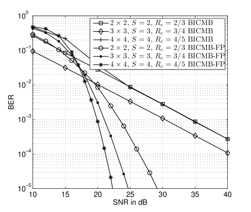
Figure 2: BER comparison between BICMB and BICMB-FP with $16$-QAM, and $64$-state punctured convolutional code.

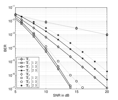
Figure 3: BER vs. SNR for BICMB-PP with $3\times 3$ $S=3$, $4$-QAM, and $4$-state $1/2$-rate convolutional code.

To compare coding gain between BICMB and BICMB-PP that achieve the full diversity order, we show in Fig. 4 the BER performances with the $4\times 4$ $S=4$ systems. The used generator polynomials of $64$-state, $1/2$ and $1/4$-rate convolutional codes are $(133,171)$ and $(117,127,155,171)$ in octal representation, respectively [11]. As shown in the figure, BICMB combined with constellation precoding shows larger coding gain with a large number of antennas and at the higher transmission rate.

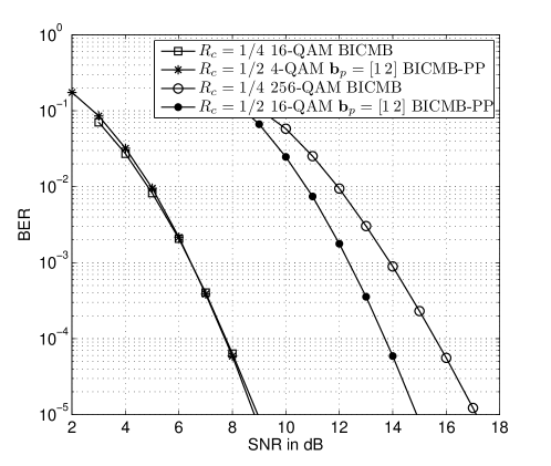
Figure 4: BER comparison between $4\times 4$ $S=4$ BICMB and BICMB-PP at $4$ and $8$ bits/channel use.

V Conclusion

We investigated the diversity order of BICMB combined with the constellation precoding scheme, by calculating pairwise error probability. Using the analysis, we presented the resulting diversity order of the given examples. The analysis can be used to determine the precoding configuration from the given BICMB implementation to get the full diversity order. We provided simulation results that proves the analysis. In addition, the simulation showed that BICMB-PP outperforms BICMB with a large number of antennas and at the higher transmission rate.

References

• [1] H. Jafarkhani, Space-Time Coding: Theory and Practice.   Cambridge University Press, 2005.
• [2] H. Sampath, P. Stoica, and A. Paulraj, “Generalized linear precoder and decoder design for MIMO channels using the weighted MMSE criterion,” IEEE Trans. Commun., vol. 49, no. 12, pp. 2198–2206, December 2001.
• [3] D. P. Palomar, J. M. Cioffi, and M. A. Lagunas, “Joint tx-rx beamforming design for multicarrier MIMO channels: A unified framework for convex optimization,” IEEE Trans. Signal Process., vol. 51, no. 9, pp. 2381–2401, September 2003.
• [4] E. Sengul, E. Akay, and E. Ayanoglu, “Diversity analysis of single and multiple beamforming,” IEEE Trans. Commun., vol. 54, no. 6, pp. 990–993, June 2006.
• [5] L. G. Ordonez, D. P. Palomar, A. Pages-Zamora, and J. R. Fonollosa, “High-SNR analytical performance of spatial multiplexing MIMO systems with CSI,” IEEE Trans. Signal Process., vol. 55, no. 11, pp. 5447–5463, November 2007.
• [6] E. Akay, E. Sengul, and E. Ayanoglu, “Bit interleaved coded multiple beamforming,” IEEE Trans. Commun., vol. 55, no. 9, pp. 1802–1811, September 2007.
• [7] E. Akay, H. J. Park, and E. Ayanoglu, “On bit-interleaved coded multiple beamforming,” 2008, arXiv: 0807.2464. [Online]. Available: http://arxiv.org
• [8] H. J. Park and E. Ayanoglu, “Diversity analysis of bit-interleaved coded multiple beamforming,” in Proc. IEEE ICC ‘09, Dresden, Germany, June 2009.
• [9] ——, “Constellation precoded beamforming,” 2009, arXiv:0903.4738v1. [Online]. Available: http://arxiv.org
• [10] ——, “Constellation precoded beamforming,” in Proc. IEEE Globecom ‘09, Honolulu, HI, November 2009.
• [11] P. Frenger, P. Orten, and T. Ottosson, “Convolutional codes with optimum distance spectrum,” IEEE Commun. Lett., vol. 3, no. 11, pp. 317–319, November 1999.