Coherent structures in fully-developed pipe turbulence

A. P. Willis,   Y. Hwang,   C. Cossu

Résumé :

Un profil moyen turbulent est prescrit dans une conduite cylindrique, en adéquation avec les observations expérimentales. Nous considérons ensuite la nature des perturbations à cet écoulement synthétique. Le calcul des croissances optimales prédit deux types de structures, associées respectivement aux structures de proche-paroi et de grande échelle. Un excellent accord quantitatif est trouvé avec les résultats expérimentaux quant à la longueur d’onde transversale. La réponse harmonique est également étudiée, et la croissance linéaire observée comparée á des simulations numériques directes de turbulence forcée. Malgré de l’hypothèse simple de type ‘Eddy viscosity’, cette approche linéaire prédit efficacement la croissance spectaculaire des modes de grande échelle au coeur de l’écoulement.

Abstract :

A turbulent mean profile for pipe flow is prescribed which closely matches experimental observations. The nature of perturbations superimposed upon this profile is then considered. Optimal growth calculations predict two distinct classes of structures, clearly associated with near-wall and large-scale structures. Quantitative correspondence of the spanwise wavelength of wall-structures with experimental observations is very good. The response to harmonic forcing is also considered, and the linear growth tested with direct numerical simulation of forced turbulence. Despite the very simple eddy viscosity assumption, this linear approach predicts well the surprisingly large growth of outer-scale modes in the bulk flow.

Mots clefs : Turbulence, Optimal growth, Pipe flow

1 Introduction

The discovery of nonlinear solutions to the Navier–Stokes equations for Pipe and Couette geometries has led to significant progress of late. For pipe flow, these travelling wave solutions were discovered by adding a forcing to the Navier–Stokes equations to induce axially independent rolls. As the forcing is increased a three-dimensional wave instability arises. Three-dimensional states could then be traced back, using continuation methods, to the original equations upon reduction of the forcing [1, 2]. Whilst successful at finding the first nonlinear states, the nature of this method leads to solutions that are only just self-sustained. As a consequence, the majority of known solutions (of the sinuous variety) were shown to be characteristic of the boundary between laminar and turbulent states. Initial states either side of this boundary develop into either turbulence or relaminarise [3, 4, 5, 6]. Only later were higher branches found (being also highly symmetric) with higher friction factors typical of turbulence [7]. The highly organised structure of these states, however, does not appear to be typical of turbulence, nor do they display the strongly decelerated core of the mean flow. It is perhaps more intuitive, therefore, that one should begin with perturbations to this mean flow.

2 Method

Here we consider perturbations to a close approximation to the mean flow profile for pipe flow. The equations are normalised by the bulk flow speed $U_{b}$ and the radius of the pipe $R$. Reynolds numbers are defined $Re=2\,U_{b}R/\nu$ and $Re_{\tau}=u_{\tau}R/\nu$, where the wall velocity $u_{\tau}=(\nu\,\partial_{r}U(r))^{\frac{1}{2}}|_{r=R}$ is derived from the mean stress at the boundary. The mean profile $U(r)$ is inverted from the $\theta$,$z$-averaged Navier–Stokes equations

$$0=-\partial_{z}P+\frac{1}{Re}\left(\frac{1}{r}+\partial_{r}\right)(\nu_{T}\partial_{r}U),\qquad B=-\partial_{z}P,$$ (1)

where the normalised effective viscosity is $\nu_{T}(y)=1+E(y)$, and $y=1-r$ is the distance from the pipe wall. The radially dependent eddy viscosity is prescribed ([8], after [9]),

$$E(y)=\frac{1}{2}\left\{1+\frac{\kappa^{2}\hat{R}^{2}\hat{B}}{9}[2y-y^{2}]^{2}(3-4y+2y^{2})^{2}\left[1-\exp\left(\frac{-y\hat{R}\sqrt{\hat{B}}}{A^{+}}\right)\right]\right\}^{\frac{1}{2}}-\frac{1}{2}\,.$$

We have updated the fitting parameters $A^{+}=27$ and $\kappa=0.42$ to be compatible with the observations of [10] and different scalings lead to the adjusted parameters $\hat{R}=Re\,/\,2$,  $\hat{B}=2\,B$.

Perturbations, $u$, to the mean profile are first considered in the linear framework. The Navier–Stokes equations with radially-dependent viscosity are linearised about $U(y)$; note that the perturbations about $U$ are also subject to the elevated effective viscosity. Rather than the usual progression to Orr–Sommerfeld–Squire form, eigenvalues and eigenvectors are found directly from the linearised primitive variable system with explicit solenoidal condition. Given the eigenfunctions and eigenvalues, using standard methods [11] one may calculate the optimal growth,

$$G(\alpha,m;t)=\max_{\mbox{\boldmath$u$}_{0}}\,\frac{||\mbox{\boldmath$u$}(t)||}{||\mbox{\boldmath$u$}_{0}||}\quad\mbox{ and }\quad G_{\mathrm{max}}=\max_{t}{G(t)}.$$ (2)

The wavelengths of the perturbations are $\lambda_{z}=2\pi/\alpha$ (streamwise) and $\lambda_{\theta}=2\pi/m$ in azimuth (spanwise). Harmonic forcing is also considered in the following discussion. For a forcing of the form $\mbox{\boldmath$f$}(t)=\mbox{\boldmath$\tilde{f}$}\,{\mathrm{e}}^{{\mathrm{i}}\omega t}$, a harmonic response $\mbox{\boldmath$u$}(t)=\mbox{\boldmath$\tilde{u}$}\,{\mathrm{e}}^{{\mathrm{i}}\omega t}$ is expected. The optimal response is then

$$R(\alpha,m;\omega)=\max_{\mbox{\boldmath$\tilde{f}$}}\,\frac{||\mbox{\boldmath$\tilde{u}$}||}{||\mbox{\boldmath$\tilde{f}$}||}\,\quad\mbox{ and }\quad R_{\mathrm{max}}=\max_{\omega}{R(\omega)}.$$ (3)

The eigenfunction calculations were performed with up to $N=200$ points on $r\in[0,1]$ using a Chebyshev collocation method. The number of (non-infinite) eigenvalues plus vectors obtained, being the number of degrees of freedom, is $2\,N-3$. Of these, 95% were kept for the optimal growth analysis. At the highest $Re=10^{6}$, for which $Re_{\tau}=19200$, the power spectral drop-off of the optimal mode was of $8$ orders of magnitude (for both ‘inner’ and ‘outer’ modes, see below).

3 Results

The structure of optimal modes in strongly sheared flows is well known to reflect the lift-up mechanism, whereby rolls aligned with the flow raise slow fluid from the boundary into the faster flow, leading to extended streaks. While shearing is certainly present in the turbulent flow, it is subject to a significantly larger effective viscosity, $\nu_{T}(r)$.

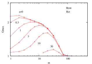
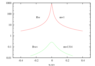
Optimal growths relative to the turbulent profile (figure 1) are significantly smaller than for the laminar case, although the greatest growth still occurs for the largest mode $m=1$. For the turbulent case, however, $\nu_{T}$ reduces to the laminar value as one approaches the wall, and growth of similar magnitude is also possible in the boundary region, provided that the length scale is not so small that diffusion again dominates.

Figure 1: Left: Optimal growth at moderate Reynolds numbers. While the peak is for $m=1$, it is clear that for larger $\alpha$ only modes of larger $m$ persist. Right: At large $Re$ a distinct peak appears at large $m$.

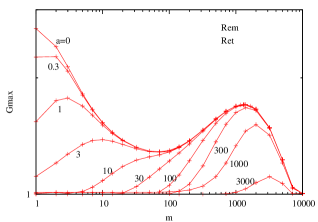
This secondary peak, for which rolls are located close to the wall, is shown in figure 2 to scale in ‘inner’ units, where in the absence of any other length scale, all units are inferred from the stress at the wall and the kinematic viscosity, $r=r^{+}\nu/u_{\tau}$, $t=t^{+}\nu/u_{\tau}^{2}$. It is clear from the figure that such scaling is appropriate at high $Re_{\tau}$, where the $G_{\mathrm{max}}$ collapse with a peak for $\lambda^{+}_{\theta}=2\pi\,Re_{\tau}/m$ at $92$.

Figure 2: Left: An inner peak occurs for spanwise wavelength $\lambda_{\theta}^{+}=92$. Right: The time $T^{+}$ s.t. $G(T)=G_{\mathrm{max}}$.

This peak in spanwise wavelength compares very favourably with experimental results. Using apparatus flush with the floor of the Utah desert [12] using smoke visualisation, a peak at was found at $\lambda^{+}=93$, for a $Re_{\tau}$ as large as $1.5\times 10^{6}$. In [13] similar values ($\pm 10$) were observed for $Re_{\tau}$ in the range $1000$ to $5000$. Our predicted value $\lambda^{+}=92$ is in excellent agreement. In the present study, this secondary inner peak is observed to be distinct from the large-scale peak ($m=1$) for $Re_{\tau}$ of order $1000$, and $\lambda_{\theta}^{+}$ being immediately close to the above value from the outset. Indeed, at lower $Re_{\tau}$, far before the peak becomes distinct for the $\alpha=0$ case, it is clear that modes of finite streamwise extent select similar $\lambda_{\theta}^{+}$.

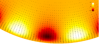
In figure 3 the optimal initial condition and response are plotted for the case $Re=5300$ ($Re_{\tau}\approx 180$) for $m=12$ ($\lambda_{\theta}^{+}\approx 98$). The rolls are typical of those of the wall mode at much greater $Re$.

Figure 3: Structure of the optimal inner-mode (left) and its response (right). Each is normalised by the maximum of $|\mbox{\boldmath$u$}|$. The initial condition consists of rolls, and the response is dominated by streaks.

The growth of an initial condition is all very well, but how easy is it to invoke such an initial condition? The response to streamwise independent forcing is plotted over a range of harmonic frequencies, $\omega$, in figure 4. The steady forcing, $\omega=0$, is most effective at generating a response for this case. While this is not true for non-zero $\alpha$, the peak response remained smaller than that for the axially independent case in all our calcuations.

Figure 4: Response to harmonic forcing; $Re_{\tau}=19200$. For $\alpha=0$, steady forcing is largest ($\omega=0$). The outer mode ($m=1$) is many orders more responsive for all moderate $\omega$ than the inner mode ($m=1314$).

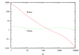
The code described in [14] has been modified to include radially dependent viscosity. The extreme difference in response to forcing different $m$ modes was verified by timestepping relative to the prescribed mean profile. The structure of the optimal force $\tilde{f}$, however, is essentially identical to that of the optimal growth initial condition $\mbox{\boldmath$u$}_{0}$ (see figure 3); similarly for their respective responses.

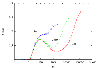
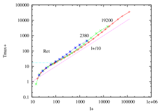
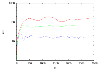
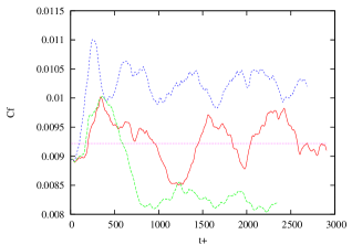
Unlike the transient growth, steady forcing provides a convenient platform for testing the model, whereby statistical measures averaged over much longer times may be accumulated. Consider the timestepped velocity field, $\mbox{\boldmath$u$}(t)$, obtained from direct numerical simulation of the original Navier–Stokes equations subject to a forcing $\tilde{f}$. Then $\mbox{\boldmath$u$}_{f}(t)=(\mbox{\boldmath$u$}(t)\cdot\mbox{\boldmath$\hat{\tilde{u}}$})\,\mbox{\boldmath$\hat{\tilde{u}}$}$ is the component of $\mbox{\boldmath$u$}(t)$ in the direction of the the expected normalised response field $\hat{\tilde{u}}$. The observed quantity $||\mbox{\boldmath$u$}_{f}(t)||/||\mbox{\boldmath$\tilde{f}$}||$ may be compared with the expected response $R_{\mathrm{max}}$. Figure 5 shows the response of the turbulent flow $Re=5300$, computed in a domain of length $10$ radii ($\lambda_{z}^{+}\approx 1800$) at a resolution $(60,\pm 64,\pm 64)$ before dealiasing. The calculations clearly demonstrate that large amplification may occur, as predicted by the model. Note also that for intermediate forcing, drag reduction is possible.

Figure 5: Response of a turbulent flow to forcing; $Re_{\tau}\approx 180$, $\alpha=0,m=1$ and $||\mbox{\boldmath$\tilde{f}$}||^{2}=10^{-6},10^{-5},10^{-4}$. Here $||\cdot||^{2}=\frac{1}{2}\int|\cdot|^{2}{\mathrm{d}}V$. The expected $R_{\mathrm{max}}$ is 280. A similar order value is achieved for $||\mbox{\boldmath$\tilde{f}$}||^{2}=10^{-6}$ and decreases as the force increases. The amplitude of the induced flow is already as large as 5 to 10% of the mean flow for all cases. The forcing has a significant affect on the skin-friction coefficient $C_{f}=2(u_{\tau}/U_{b})^{2}$, the horizontal line being the unforced average.

4 Conclusions

The model has been shown to successfully predict large growth, to good quantitive agreement, despite the assumptions of linearity upon a turbulent state and the isotropic eddy viscosity assumption. It shows the huge response to forcing of large scale modes, and accurately predicts the peak spanwise wavelength, $\lambda_{\theta}^{+}=92$, of the near-wall modes.

Analogue studies for optimal growth in turbulent channels [15, 16], the boundary layer [17] and the Couette flow [18], all show close spanwise wavelengths for the wall mode. It is surprising, however, that the optimal growth calculations suggest small growth of the wall modes, despite clear observational evidence that such structures exist.

The results from harmonic forcing, on the other hand, suggest that the large scale modes are easily excited. Such relative difficulty of forcing motion on small scales has consequences for control of turbulence. It clearly requires considerable effort to locally manipulate structures in the neighbourhood of the wall. It is possible that it is more straight forward to control indirectly via forcing of larger, or possibly even very large scales, taking advantage of the much greater linear response. Indeed, such a possiblity has been shown in principle for channel flow [19], and is verified here for a significantly larger ratio of ‘large’ (imposed roll) to ‘small’ (streak spacing) scales. The nature of suppression by a large-scale motion deserves further investigation.