Generation of Werner-like stationary states of two qubits in a thermal reservoir

Abstract

The dynamics of entanglement between two-level atoms immersed in the common photon reservoir at finite temperature is investigated. It is shown that in the regime of strong correlations there are nontrivial asymptotic states which can be interpreted in terms of thermal generalization of Werner states.

I Introduction

Entanglement generation by the indirect interaction between otherwise decoupled systems has been discussed in the literature mainly in the case of two-level atoms interacting with the common vacuum. The idea that dissipation can create rather then destroy entanglement in some systems, was put forward in several publications Plenio ; Kim ; SM ; PH . In particular, the effect of spontaneous emission on destruction and production of entanglement was discussed J ; FT1 ; FT2 ; JJ1 . When the two atoms are separated by a distance small compared to the radiation wave length, the collective properties of two-atomic systems can alter the decay process compared with the single atom. It was already shown by Dicke Di that there are states with enhanced emission rates (superradiant states) and such that the emission rate is reduced (subradiant states). (In the case of multi-atomic systems, similar collective effects described by Tavis-Cummings interaction TC can generate collective multiqubit entanglement RSR ). When the emission rate is reduced, two-atom system can decohere slower compared with individual atoms and some amount of initial entanglement can be preserved or even created by the indirect interaction between atoms. The analogous effect of production of entanglement was studied in a system of two-level atoms interacting with a squeezed vacuum. In that case, the squeezed vacuum is a source of nonclassical correlations which are essential for creation of entanglement TF . The general condition under which entanglement can be induced by interaction with environment was also discovered BFP .

The case of two atoms immersed in a common thermal reservoir was also investigated BF ; ZY ; L . In particular, Benatti and Floreanini BF have discussed the dynamics of two independent atoms interacting with the reservoir of scalar particles at finite temperature and found the interesting behavior of the system. If the atoms are at finite separation, there is a temperature of the reservoir below which entanglement generation occurs. Moreover, for the vanishing separation, the entanglement thus generated persists in the asymptotic state.

In the present paper, we study the similar model but from a different perspective. We consider the system of two-level atoms interacting with the photon reservoir at fixed temperature. As in the vacuum case, the collective properties of the atomic system can alter the decay process compared with the single atom. There are states with enhanced emission rates and such that the emission rate is reduced. The important example of the latter is the singlet state $|{a}\rangle$ i.e. antisymmetric superposition constructed from energy levels of considered atoms. As we show, in the regime of strong correlations the singlet state is decoupled from the environment and therefore is stable. In our considerations we focus on this case and investigate the stationary asymptotic states of the system. In turns out that the asymptotic states are parametrized by the fidelity $F$ of the initial state $\varrho$ with respect to the state $|{a}\rangle$ (or the overlap of $\varrho$ with singlet $|{a}\rangle$) and the temperature $T$ of the photon reservoir. We identify the asymptotic states as the thermal generalization of Werner states i.e. mixture of singlet state and Gibbs equilibrium state at the temperature $T$ with the appropriate probability. (The standard Werner states W are recovered in the limit of infinite temperature). Depending on the initial fidelity some of the asymptotic states are entangled. We calculate the amount of the asymptotic entanglement using a concurrence as its measure. We also show that if the initial fidelity is greater or equal to $1/2$, then for every finite temperature of the reservoir the asymptotic entanglement is non-zero. On the other hand, for fidelity less then $1/2$ there is the critical temperature below which the asymptotic states are entangled whereas for higher temperatures all stationary states are separable.

Since the initial states with the same fidelity can be separable or entangled, the dynamics given by the interaction with the reservoir manifests differently with respect to the entanglement properties of the system. It can create entanglement when the initial states are separable, disentangle initially entangled states, preserve some part of initial entanglement or even increase the initial entanglement of some states. We show on specific examples that this behavior of the dynamics really occurs. In particular, pure product states with orthogonal factor vectors become entangled in every temperature, whereas for other product states there is the critical temperature for creation of entanglement. Similar phenomenon can be observed if the initial state is mixed. For example in the case of Gibbs equilibrium state at the temperature $T_{0}$ which differs from the temperature $T$ of the reservoir, the creation of asymptotic entanglement happens if $T_{0}$ is much higher then $T$. On the other hand, entangled initial states with maximal amount of entanglement can preserve some initial entanglement or can disentangle completely. It is worth to stress that this different behavior with respect to the thermal noise can happen for locally equivalent initial states, so by performing only local operations one can protect as much entanglement as possible. When the initial states are not maximally entangled, then the thermal noise can in some cases create entanglement which adds to the initial one, although during the evolution the purity is decreasing.

II Two qubits dynamics

We start with the sketch of the derivation of the dynamical equation describing the evolution of the system of atoms immersed in the thermal reservoir (for details see e.g. FT ).

Consider two-level atoms $A$ and $B$ with ground states $|{0}\rangle_{j}$ and excited states $|{1}\rangle_{j}$ ($j=A,\,B$), interacting with photon reservoir at temperature $T$. The dynamics of the combined system consisting of the atoms and the quantum electromagnetic field is given by the Hamiltonian

$$H_{\mathrm{SF}}=H_{0}+H_{I}$$

where $H_{0}$ is the sum of free Hamiltonians of the atoms and the field and $H_{I}$ describes the interaction between the atoms and photons in the electric dipole approximation. Since we are interested in the dynamics of the system of atoms, we take the partial trace over field variables and find that the reduced density matrix of the atomic system satisfies some integro-differential equation which can be simplified by employing the Born approximation (the interaction between the atoms and the field is so weak that there is no back reaction effect of the atoms on the field). Under this approximation, the evolution of the density matrix depends on the first- and second-order correlation functions of the field operators in the thermal equilibrium state at temperature $T$. Employing further the rotating-wave approximation in which we ignore all terms oscillating at higher frequencies and assuming that the correlation time of the photon reservoir is short (the Markov approximation), we arrive at the result that the influence of reservoir on the system of atoms can be described by dynamical semi-group AL with Lindblad generator $L=-i\,[H,\,\cdot]+L_{\mathrm{D}}$, where

$$H=\frac{\omega}{2}\sum\limits_{j=A,B}\sigma_{3}^{j}+\sum\limits_{j,\,k=A,B\atop j\neq k}\Omega_{jk}\sigma_{+}^{j}\sigma_{-}^{k}$$ (II.1)

and

$$\begin{split}L_{\mathrm{D}}\varrho=&\frac{1}{2}\sum\limits_{j,\,k=A,\,B}\Gamma_{jk}^{\downarrow}\,\left(2\sigma_{-}^{j}\varrho\sigma_{+}^{k}-\sigma_{+}^{k}\sigma_{-}^{j}\varrho-\varrho\sigma_{+}^{k}\sigma_{-}^{j}\right)\\ &\hskip 25.60747pt+\Gamma_{jk}^{\uparrow}\,\left(2\sigma_{+}^{j}\varrho\sigma_{-}^{k}-\sigma_{-}^{k}\sigma_{+}^{j}\varrho-\varrho\sigma_{-}^{k}\sigma_{+}^{j}\right)\end{split}$$ (II.2)

Here

$$\sigma_{\pm}^{A}=\sigma_{\pm}\otimes\openone,\quad\sigma_{\pm}^{B}=\openone\otimes\sigma_{\pm},\quad\sigma_{3}^{A}=\sigma_{3}\otimes\openone,\quad\sigma_{3}^{B}=\openone\otimes\sigma_{3}$$

In the Hamiltonian (II.1), $\omega$ is the frequency of the transition $|{0}\rangle_{j}\to|{1}\rangle_{j}$ ($j=A,\,B$) and $\Omega_{AB}=\Omega_{BA}=\Omega$ describes interatomic coupling by the dipole-dipole interaction. On the other hand, dissipative dynamics is given by the generator (II.2) with

$$\Gamma_{jk}^{\downarrow}=\gamma_{jk}\,(1+\langle{n}\rangle),\quad\Gamma_{jk}^{\uparrow}=\gamma_{jk}\,\langle{n}\rangle$$

where

$$\langle{n}\rangle=\frac{e^{-\beta\omega}}{1-e^{-\beta\omega}},\quad\beta=\frac{1}{T}$$

is the mean number of photons, and

$$\gamma_{AA}=\gamma_{BB}=\gamma_{0},\quad\gamma_{AB}=\gamma_{BA}=\gamma$$ (II.3)

In the above equalities, $\gamma_{0}$ is the single atom spontaneous emission rate, and $\gamma=G\gamma_{0}$ is the collective damping constant. In the model considered, $G$ is the function of the interatomic distance $R$, and $G$ is small for large separation of atoms. On the other hand, $G\to 1$ when $R$ is small.

The master equation

$$\frac{d\varrho}{dt}=L\varrho$$ (II.4)

giving the time evolution of a density matrix of the system of two-level atoms can be used to obtain the equations for its matrix elements with respect to some basis. To simplify the calculations one can work in the basis of collective states in the Hilbert space $\mathbb{C}^{2}\otimes\mathbb{C}^{2}$ FT , given by product vectors

$$|{e}\rangle=|{1}\rangle_{A}\otimes|{1}\rangle_{B},\quad|{g}\rangle=|{0}\rangle_{A}\otimes|{0}\rangle_{B}$$ (II.5)

symmetric superposition

$$|{s}\rangle=\frac{1}{\sqrt{2}}\left(|{0}\rangle_{A}\otimes|{1}\rangle_{B}+|{1}\rangle_{A}\otimes|{0}\rangle_{B}\right)$$ (II.6)

and antisymmetric superposition

$$|{a}\rangle=\frac{1}{\sqrt{2}}\left(|{1}\rangle_{A}\otimes|{0}\rangle_{B}-|{0}\rangle_{A}\otimes|{1}\rangle_{B}\right)$$ (II.7)

In the basis of collective states, two-atom system can be treated as a single four-level system with ground state $|{g}\rangle$, excited state $|{e}\rangle$ and two intermediate states $|{s}\rangle$ and $|{a}\rangle$. From (II.4) it follows that the matrix elements of the state $\varrho$ with respect to the basis $|{e}\rangle,\,|{s}\rangle,\,|{a}\rangle,\,|{g}\rangle$ satisfy the equations which can be grouped into decoupled systems of differential equations. So for diagonal matrix elements we obtain

$$\begin{split}\frac{d\rho_{ee}}{dt}&=(\gamma_{0}-\gamma)\langle{n}\rangle\rho_{aa}-2\gamma_{0}(1+\langle{n}\rangle)\rho_{ee}+(\gamma_{0}+\gamma)\langle{n}\rangle\rho_{ss}\\ \frac{d\rho_{ss}}{dt}&=-(\gamma_{0}+\gamma)[(1+\langle{n}\rangle)\rho_{ee}-(1+2\langle{n}\rangle)\rho_{ss}+\langle{n}\rangle\rho_{gg}]\\ \frac{d\rho_{aa}}{dt}&=-(\gamma_{0}-\gamma)[(1+2\langle{n}\rangle)\rho_{aa}-(1+\langle{n}\rangle)\rho_{ee}-\langle{n}\rangle\rho_{gg}]\\ \frac{d\rho_{gg}}{dt}&=(\gamma_{0}-\gamma)(1+\langle{n}\rangle)\rho_{aa}+(\gamma_{0}+\gamma)\rho_{ss}-2\gamma_{0}\langle{n}\rangle\rho_{gg}\end{split}$$ (II.8)

On the other hand, the elements $\rho_{es}$ and $\rho_{sg}$ are connected by the equations

$$\begin{split}\frac{d\rho_{es}}{dt}&=(\gamma_{0}+\gamma)\langle{n}\rangle\rho_{sg}-\frac{1}{2}[(1+2\langle{n}\rangle)\gamma\\ &\hskip 11.38109pt+(3+4\langle{n}\rangle)\gamma_{0}-2i(\omega-\Omega)]\rho_{es}\\ \frac{d\rho_{sg}}{dt}&=(\gamma_{0}+\gamma)(1+\langle{n}\rangle)\rho_{es}-\frac{1}{2}[(1+2\langle{n}\rangle)\gamma\\ &\hskip 11.38109pt+(1+4\langle{n}\rangle)\gamma_{0}+2i(\omega+\Omega)]\rho_{sg}\end{split}$$ (II.9)

and similarly, the elements $\rho_{ea}$ and $\rho_{ag}$ satisfy

$$\begin{split}\frac{d\rho_{ea}}{dt}&=-(\gamma_{0}-\gamma)\langle{n}\rangle\rho_{ag}+\frac{1}{2}[(1+2\langle{n}\rangle)\gamma\\ &\hskip 11.38109pt-(3+4\langle{n}\rangle)\gamma_{0}-2i(\omega+\Omega)]\rho_{ea}\\ \frac{d\rho_{ag}}{dt}&=-(\gamma_{0}-\gamma)(1+\langle{n}\rangle)\rho_{ea}-\frac{1}{2}[(1+4\langle{n}\rangle)\gamma_{0}\\ &\hskip 11.38109pt-(1+2\langle{n}\rangle)\gamma+2i(\omega-\Omega)]\rho_{ag}\end{split}$$ (II.10)

Finally

$$\frac{d\rho_{eg}}{dt}=-[(1+2\langle{n}\rangle)\gamma_{0}+2i\omega]\rho_{eg}$$ (II.11)

and

$$\frac{d\rho_{sa}}{dt}=-[(1+2\langle{n}\rangle)\gamma_{0}+2i\Omega]\rho_{sa}$$ (II.12)

The equations for the remaining matrix elements can be obtained by using hermiticity of $\varrho$.

From the equations (II.8) it follows that similarly as in the zero temperature case (see e.g. FT ), the system of atoms prepared in the symmetric state $|{s}\rangle$ decays with enhanced rate $\gamma_{0}+\gamma$, whereas antisymmetric initial state $|{a}\rangle$ leads to the reduced rate $\gamma_{0}-\gamma$. In the limiting case of strongly correlated atoms we can put $\gamma=\gamma_{0}$, so the state $|{a}\rangle$ is completely decoupled from the photon reservoir. One can also check that the master equation (II.4) describes two types of time evolution of the atomic system, depending on the relation between $\gamma$ and $\gamma_{0}$. When $\gamma<\gamma_{0}$, there is a unique asymptotic state of the system, which is the Gibbs state

$$\varrho_{\beta}=e^{-\beta H_{0}}\big{/}\mathrm{tr}\,\,e^{-\beta H_{0}},\quad H_{0}=\frac{\omega}{2}\sum\limits_{j=A,B}\sigma_{3}^{j}$$ (II.13)

The state (II.13) is separable and describes thermal equilibrium of atoms interacting with photon reservoir. In the regime of strong correlations, $\gamma=\gamma_{0}$ and we show that there are nontrivial asymptotic stationary states which can be parametrized by matrix elements $\rho_{aa}$ of the initial state.

III Strongly correlated qubits and nontrivial asymptotic states

When $\gamma=\gamma_{0}$, equations (II.8) - (II.12) simplify and one can check that the solutions of (II.9) - (II.12) asymptotically vanish, so the only contribution to the stationary states $\varrho_{\mathrm{as}}$ comes from the matrix elements $\rho_{aa},\,\rho_{ss},\rho_{ee}$ and $\rho_{gg}$. Notice that

$$\frac{d\rho_{aa}}{dt}=0,\quad\text{so}\quad\rho_{aa}(t)=\rho_{aa}(0)=F$$

where

$$F=\langle{a}|\varrho|{a}\rangle$$

is the fidelity of the initial state $\varrho$ with respect to the singlet state $|{a}\rangle$. Hence $(\varrho_{\mathrm{as}})_{aa}=F$ and after a long elementary calculation, we obtain that

$$\begin{split}(\varrho_{\mathrm{as}})_{ee}&=\frac{e^{-2\beta\omega}}{u(\beta)}\;(1-F)\\ (\varrho_{\mathrm{as}})_{ss}&=\frac{e^{-\beta\omega}}{u(\beta)}\;(1-F)\\ (\varrho_{\mathrm{as}})_{gg}&=\frac{1}{u(\beta)}\;(1-F)\end{split}$$ (III.1)

where

$$u(\beta)=1+e^{-\beta\omega}+e^{-2\beta\omega}$$

In the canonical basis

$$|{1}\rangle_{A}\otimes|{1}\rangle_{B},\;|{1}\rangle_{A}\otimes|{0}\rangle_{B},\;|{0}\rangle_{A}\otimes|{1}\rangle_{B},\;|{0}\rangle_{A}\otimes|{0}\rangle_{B}$$

the non-zero matrix elements of the asymptotic state reads

$$\begin{split}(\varrho_{\mathrm{as}})_{11}&=\frac{e^{-2\beta\omega}}{u(\beta)}\;(1-F)\\ (\varrho_{\mathrm{as}})_{22}&=\frac{e^{-\beta\omega}}{2u(\beta)}\;(1-F)+\frac{F}{2}\\ (\varrho_{\mathrm{as}})_{23}&=\frac{e^{-\beta\omega}}{2u(\beta)}\;(1-F)-\frac{F}{2}\\ (\varrho_{\mathrm{as}})_{44}&=\frac{1}{u(\beta)}\;(1-F)\end{split}$$ (III.2)

and $(\varrho_{\mathrm{as}})_{33}=(\varrho_{\mathrm{as}})_{22}$.

The asymptotic state $\varrho_{\mathrm{as}}$ defined by (III.2) exists for any initial state and for the fixed temperature of the photon reservoir it depends only on the initial fidelity i.e. $\varrho_{\mathrm{as}}=\varrho_{\mathrm{as}}(F)$. If we define the threshold fidelity $F_{\beta}$ by

$$F_{\beta}=\frac{e^{-\beta\omega}}{(1+e^{-\beta\omega})^{2}}$$

then one can check that:
(1) $\varrho_{\mathrm{as}}(F_{\beta})$ equals the the Gibbs state $\varrho_{\beta}$,
(2) for $F>F_{\beta}$, $\varrho_{\mathrm{as}}(F)$ equals to the thermal generalization of the Werner state

$$W_{\beta}=(1-p)\,\varrho_{\beta}+p\,|{a}\rangle\langle{a}|$$ (III.3)

where the mixing probability $p$ depends on the fidelity of the initial state and temperature of the reservoir :

$$p=\frac{(1+e^{-\beta\omega})^{2}\,F-e^{-\beta\omega}}{u(\beta)}$$ (III.4)

(3) for $F<F_{\beta}$, the state $\varrho_{\mathrm{as}}$ cannot be expressed as the Werner state (III.3)

Notice that in the limit $\beta\to 0$ (or $T\to\infty$) we obtain the standard Werner state W , hence the dynamical generation of such states occurs due to the interaction with the environment with maximal noise JJ . The entanglement properties of the asymptotic state will be discussed in the next section.

IV Asymptotic entanglement

We start with the characterization of entanglement of the thermal Werner state $W_{\beta}$. The simplest way to do this is to use Wootters concurrence Woot defined for any two-qubit state $\varrho$ as

$$C(\varrho)=\max\left(\,0,\sqrt{\lambda_{1}}-\sqrt{\lambda_{2}}-\sqrt{\lambda_{3}}-\sqrt{\lambda_{4}}\,\right)$$ (IV.1)

where $\lambda_{1}>\lambda_{2}>\lambda_{3}>\lambda_{4}$ are the eigenvalues of the matrix $\varrho\widetilde{\varrho}$ with $\widetilde{\varrho}$ given by

$$\widetilde{\varrho}=\sigma_{2}\otimes\sigma_{2}\,\overline{\varrho}\,\sigma_{2}\otimes\sigma_{2}$$

where $\overline{\varrho}$ denotes complex conjugation of the matrix $\varrho$. By a direct calculation one obtains that for the states

$$\varrho=\begin{pmatrix}\varrho_{11}&0&0&0\\ 0&\varrho_{22}&\varrho_{23}&0\\ 0&\varrho_{32}&\varrho_{33}&0\\ 0&0&0&\varrho_{44}\end{pmatrix}$$ (IV.2)

the concurrence is given by the simple function

$$C(\varrho)=\max\,\left(\,0,\;2\,(|\varrho_{23}|-\sqrt{\varrho_{11}\varrho_{44}})\;\right)$$ (IV.3)

Since the states (III.3) are of the form (IV.2), $C(W_{\beta})$ reads

$$C(W_{\beta})=\max\,\left(\,0,\;p-\frac{2e^{-\beta\omega}}{(1+e^{-\beta\omega})^{2}}\,(1-p)\,\right)$$ (IV.4)

so for

$$p>p_{0}=\frac{2e^{-\beta\omega}}{1+4e^{-\beta\omega}+e^{-2\beta\omega}}$$

thermal Werner states are entangled, and for $p\leq p_{0}$, those states are separable. Combining this result with the formula (III.4), we obtain the concurrence of the asymptotic states (see also BF ; L )

$$C_{\mathrm{as}}=\max\,\left(\,0,\,F-\frac{3}{1+2\cosh\beta\omega}\,(1-F)\;\right)$$ (IV.5)

Observe that for the fixed temperature of the reservoir the asymptotic entanglement depends only on the fidelity of the initial state. Moreover, this entanglement is non-zero for all initial states with fidelity satisfying

$$F>F_{0}=\frac{3}{4+2\cosh\beta\omega}$$ (IV.6)

Obviously, all asymptotic states with fidelity less then threshold value $F_{\beta}$ are separable.

We can also consider the interesting problem of temperature dependence of the asymptotic entanglement. Notice that for every $\beta>0$ and $F\geq 1/2$

$$F-\frac{3}{1+2\cosh\beta\omega}\,(1-F)>0$$

So the interaction of the atomic system with the reservoir at any finite temperature brings all initial states with the fidelity $F$ greater or equal to $1/2$ into the stationary entangled states. On the other hand, when the fidelity is smaller then $1/2$, there is the critical temperature i.e such temperature $T_{\mathrm{c}}$ that if $T<T_{\mathrm{c}}$ the asymptotic states are entangled whereas for $T\geq T_{\mathrm{c}}$ the asymptotic states corresponding to the same initial fidelity are separable. Simple calculation shows that

$$\frac{T_{\mathrm{c}}}{\omega}=\varphi(F)$$ (IV.7)

where for $F<1/2$

$$\varphi(F)=\left[\ln\left(\frac{\sqrt{3}\sqrt{3-8F+4F^{2}}+3-4F}{2F}\right)\right]^{-1}$$ (IV.8)

Since the states with the same fidelity can be separable or entangled, we expect that the system will behave differently depending on the initial conditions. More precisely, it can happen that unentangled atoms become entangled during the evolution and initially entangled states disentangle or remain entangled. Next we show that the above possibilities actually occur.

IV.1 Separable initial states

When the initial state is the pure product state

$$|{\Psi}\rangle=|{\varphi}\rangle\otimes|{\psi}\rangle,\quad|{\varphi}\rangle,|{\psi}\rangle\in\mathbb{C}^{2}$$ (IV.9)

then its fidelity is given by

$$F=\frac{1}{2}\left(1-|\langle{\varphi}|\psi\,\rangle|^{2}\,\right)$$ (IV.10)

If we denote $|\langle{\varphi}|\psi\,\rangle|=\alpha$, the concurrence of the asymptotic state corresponding to (IV.9) can be computed from the formula

$$C_{\mathrm{as}}(\alpha)=\max\,\left(\,0,\,\frac{(1-\alpha^{2})\cosh\beta\omega-1-2\alpha^{2}}{1+2\cosh\beta\omega}\,\right)$$ (IV.11)

Figure 1: $C_{\mathrm{as}}(\alpha)$ as a function of temperature for the state (IV.9) with $\alpha=0$.

In the case when the vectors $\varphi$ and $\psi$ are orthogonal (for example $\varphi$ is the excited state of the atom $A$ and $\psi$ is the ground state of the atom $B$), $F$ is maximal and for every finite temperature the concurrence of the asymptotic state is non-zero. So the interaction with the photon reservoir creates the stationary entanglement between initially unentangled atoms. The amount of this entanglement is maximal for the zero temperature and decreases asymptotically to zero when the temperature of the reservoir increases to infinity(FIG. 1). Notice also that for $\alpha=1,\;C_{\mathrm{as}}(\alpha)$ trivially vanish. In the general case when $0<\alpha<1$, the creation of the stationary entanglement is possible only for the temperatures of the reservoir below the critical temperature, which in that case is given by the formula

$$\frac{T_{\mathrm{c}}}{\omega}=\left[\,\ln\left(\frac{\sqrt{3}\sqrt{2\alpha^{2}+\alpha^{4}}+1+2\alpha^{2}}{1-\alpha^{2}}\right)\,\right]^{-1}$$ (IV.12)

Since $T_{\mathrm{c}}$ goes to infinity when $\alpha$ goes to zero, the critical temperature can be high for some initial states, but the created entanglement is always maximal for zero temperature and vanishes for $T=T_{\mathrm{c}}$ (FIG. 2).

Figure 2: $C_{\mathrm{as}}(\alpha)$ as a function of temperature for the state (IV.9) with $\alpha=1/4$.

As the example of mixed separable initial state, consider the Gibbs state (II.13) at some temperature $T_{0}\neq T$. Notice that the fidelity $F$ of that state is given by

Figure 3: Critical temperature versus $T_{0}$.

$$F=\frac{e^{-\beta_{0}\omega}}{(1+e^{-\beta_{0}\omega})^{2}},\quad\beta_{0}=\frac{1}{T_{0}}$$ (IV.13)

and the value of $F$ is always smaller then $1/2$. So there is the critical temperature $T_{\mathrm{c}}$ of the reservoir for the creation of asymptotic entanglement and $T_{\mathrm{c}}$ depends on $T_{0}$. Explicit function describing $T_{\mathrm{c}}$ can be obtained by combining the formulas (IV.7) and (IV.13). Since the resulting function is complicated, we will not reproduce it here and show only its plot (FIG. 3). Observe that the critical temperature is always below the temperature $T_{0}$, thus in order to entangle the atomic system prepared in the Gibbs state at temperature $T_{0}$, the temperature of the photon reservoir have to be much smaller then $T_{0}$. On the other hand, the amount of the created entanglement can be computed from the formula (IV.5). Similarly as in the case of pure initial states, asymptotic concurrence is a decreasing function of temperature and vanishes at $T_{\mathrm{c}}$ (FIG. 4).

Figure 4: $C_{\mathrm{as}}$ as a function of temperature for the Gibbs state with $T_{0}/\omega=4$.

IV.2 Entangled initial states

The collective states $|{s}\rangle$ and $|{a}\rangle$ are specific instances of states with maximal possible entanglement. In the case of two qubits the set of maximally entangled states form a three-parameter family of states. As was shown in BJO , the corresponding projectors can be parametrized as follows

$$P_{a,\vartheta_{1},\vartheta_{2}}=$$

$$\frac{1}{2}\,\begin{pmatrix}a^{2}&ce^{-i\vartheta_{1}}&ce^{-i\vartheta_{2}}&-a^{2}e^{-i(\vartheta_{1}+\vartheta_{2})}\\[2.84526pt] ce^{i\vartheta_{1}}&b^{2}&b^{2}e^{i(\vartheta_{1}-\vartheta_{2})}&-ce^{-i\vartheta_{2}}\\[2.84526pt] ce^{i\vartheta_{2}}&b^{2}e^{-i(\vartheta_{1}-\vartheta_{2})}&b^{2}&-ce^{-\vartheta_{1}}\\[2.84526pt] -a^{2}e^{i(\vartheta_{1}+\vartheta_{2})}&-ce^{i\vartheta_{2}}&-ce^{i\vartheta_{1}}&a^{2}\end{pmatrix}$$ (IV.14)

where $b^{2}=1-a^{2},\;c=a\sqrt{1-a^{2}}$ and

$$a\in[0,1],\quad\vartheta_{1},\vartheta_{2}\in[0,2\pi]$$

All the states (IV.14) have concurrence equal to $1$, but

$$F=\frac{1}{2}\,(1-a^{2})\left(\,1-\cos(\vartheta_{1}-\vartheta_{2})\,\right)$$ (IV.15)

Notice that the fidelity $F$ can take all values from $0$ to $1$, depending on parameters $a$ and $\vartheta=\vartheta_{1}-\vartheta_{2}$. In particular $F>1/2$ inside the set $\mathcal{E}$ on the $(a,\vartheta)$ plane, given by

$$\mathcal{E}=\{\,0\leq a\leq\frac{1}{\sqrt{2}},\;\arccos\frac{a^{2}}{a^{2}-1}\leq\vartheta\leq 2\pi-\arccos\frac{a^{2}}{a^{2}-1}\,\}$$ (IV.16)

On the boundary of ${\mathcal{E}},\;F=1/2$ and outside this set, $F<1/2$. So all initial states (IV.14) with $(a,\vartheta_{1}-\vartheta_{2})\in{\mathcal{E}}$ remain entangled asymptotically, for any finite temperature of the reservoir. The asymptotic concurrence can be computed from the formula

$$C_{\mathrm{as}}(a,\vartheta)=\frac{2(1-a^{2})\left(\sin^{2}\frac{\displaystyle\vartheta}{\displaystyle 2}\cosh\beta\omega-\cos\vartheta\,\right)-(1+2a^{2})}{1+2\cosh\beta\omega}$$ (IV.17)

for $(a,\vartheta)\in\mathcal{E}$. Notice that for all such initial states the value of asymptotic concurrence is smaller then $1$, except antisymmetric collective state $|{a}\rangle$ which is stable during the evolution. As in the previous cases, the asymptotic concurrence is maximal for the reservoir at zero temperature, with the value given by

$$C_{\mathrm{max}}=(1-a^{2})\,\sin^{2}\frac{\displaystyle\vartheta}{\displaystyle 2},$$ (IV.18)

but in the present case, it decreases to the nonzero minimal value $C_{\mathrm{min}}$ when the temperature of the reservoir increases to infinity, and

$$C_{\mathrm{min}}=-\,\left(a^{2}+(1-a^{2})\cos\vartheta\,\right)$$ (IV.19)

For the parameters $(a,\vartheta)$ lying outside the set $\mathcal{E}$, there is the critical temperature $T_{\mathrm{c}}$ given by (IV.7) and (IV.8) for fidelity (IV.15). For $T<T_{\mathrm{c}}$, the interaction with reservoir preserves some initial entanglement, but for $T\geq T_{\mathrm{c}}$, all maximally entangled states with such parameters $a$ and $\vartheta$ disentangle asymptotically. Some initial states (IV.14) disentangle exactly to the equilibrium Gibbs states at the specific temperature $\widetilde{T}$, depending on $a$ and $\vartheta$. This interesting phenomenon can happen when

$$(1-a^{2})\,\left(\,1-\cos\vartheta\,\right)=\frac{e^{-\widetilde{\beta}\omega}}{(1+e^{-\widetilde{\beta}\omega})^{2}},\quad\widetilde{\beta}=\frac{1}{\widetilde{T}}$$ (IV.20)

This equation can be satisfied for some finite temperature $\widetilde{T}$ only if the parameters $(a,\vartheta)$ lie outside the curve

$$\vartheta=\arccos\frac{2a^{2}-1}{2\,(a^{2}-1)},\quad a\in[0,\sqrt{3}/2]$$ (IV.21)

and then

$$\widetilde{T}=\left[\,\ln\frac{a^{2}+(1-a^{2})\cos\vartheta+\sqrt{2a^{2}-1+2(1-a^{2})\cos\vartheta}}{(1-a^{2})(1-\cos\vartheta)}\,\right]^{-1}$$ (IV.22)

On the curve (IV.21), this temperature is infinite.

When the initial states are non-maximally entangled, the interaction with the photon reservoir can in some cases increase the initial entanglement. To show that this is possible, consider the class of states

$$\varrho=\begin{pmatrix}0&\hskip 8.53581pt0&\hskip 8.53581pt0&\hskip 8.53581pt0\\[5.69054pt] 0&\hskip 8.53581ptx&-\frac{\displaystyle z}{\displaystyle 2}&\hskip 8.53581pt0\\[5.69054pt] 0&-\frac{\displaystyle z}{\displaystyle 2}&1-x&\hskip 8.53581pt0\\[5.69054pt] 0&\hskip 8.53581pt0&\hskip 8.53581pt0&\hskip 8.53581pt0\end{pmatrix}$$ (IV.23)

where $x,z\in(0,1)$ are related by inequality

$$\frac{z^{2}}{4}\leq x(1-x)$$

Note that as the explicit examples of states (IV.23) we can consider the pure states

$$|{\Psi}\rangle_{\eta}=\cos\eta\;|{0}\rangle_{A}\otimes|{1}\rangle_{B}+\sin\eta\;|{1}\rangle_{A}\otimes|{0}\rangle_{B}$$ (IV.24)

with $\eta\in(\pi/2,\pi)$. The states (IV.23) are entangled with concurrence equal to $z$, and

$$F=\frac{1+z}{2}>\frac{1}{2}$$

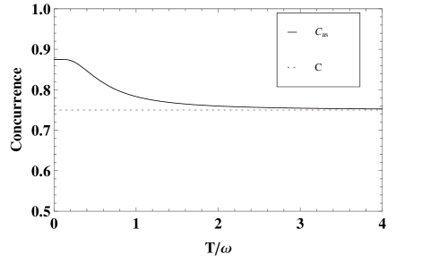
Figure 5: Asymptotic entanglement as a function of temperature for the initial state (IV.23). Here $C$ is the initial entanglement.

For every temperature of the reservoir the asymptotic concurrence is non-zero and is given by

$$C_{\mathrm{as}}(z)=z+\frac{(1-z)(\cosh\beta\omega-1)}{1+2\cosh\beta\omega}$$ (IV.25)

So it is greater then the initial concurrence and the maximal production of the additional entanglement happens at zero temperature (FIG. 5). In that case

$$C_{\mathrm{max}}(z)=z+\frac{1-z}{2}$$

Observe also that when $T\to\infty$, $C_{\mathrm{as}}(z)\to z$, so in the reservoir at infinite temperature the initial entanglement is exactly preserved JJ .

V Conclusions

We have investigated the dynamics of two-level atoms immersed in the photon reservoir at finite temperature $T$. In the regime of strong correlations between the atoms, there are nontrivial stationary asymptotic states which are parametrized by the fidelity $F$ i.e. the overlap of the initial state of the atoms with the singlet state and the temperature $T$. For the values of $F$ above the threshold fidelity, these states can be identified with thermal Werner states, which are natural generalizations of standard Werner states. Depending on $F$ and $T$, the asymptotic states can be separable or entangled. Thus the dynamics describes the process of creation of entanglement or the phenomenon of disentanglement. Concerning generation of entanglement it is worth to stress that there exists a critical temperature above which the entanglement cannot be created. Besides, even in the case of generation of entanglement, the temperature diminishes its production. The maximal value of entanglement is obtained for the case of zero temperature. On the other hand, in the process of disentanglement some part of initial entanglement can be preserved but we can also find such entangled initial states that disentangle exactly to the Gibbs equilibrium state.

References

- (1) M.B. Plenio, S.F. Huelga, Phys. Rev. Lett. 88, 197901(2002).
- (2) M.S. Kim, J. Lee, D. Ahn, P.L, Knight, Phys. Rev. A65, 040101(2002).
- (3) S. Schneider, G.J. Milburn, Phys. Rev. A 65, 042107(2002).
- (4) M. B. Plenio, S.F. Huelga, A. Beige, P.L. Knight, Phys. Rev. A 59, 2468(1999).
- (5) L. Jakóbczyk, J. Phys. A 35, 6383(2002); 36, 1537(2003), Corrigendum.
- (6) Z. Ficek, R. Tanaś, J. Mod. Opt. 50, 2765(2003).
- (7) R. Tanaś, Z. Ficek, J. Opt. B, 6, S90(2004).
- (8) L. Jakóbczyk, J. Jamróz, Phys. Lett. A 318, 318(2003).
- (9) R.H. Dicke, Phys. Rev. 93, 99(1954).
- (10) M. Tavis, F.W. Cummings, Phys. Rev. 170, 379(1968).
- (11) A. Retzker, E. Solano, B. Reznik, Phys. Rev. A 75, 022312(2007).
- (12) R. Tanaś, Z. Ficek, J. Opt. B 6, S610(2004).
- (13) F. Benatii, R. Floreanini, M. Piani, Phys. Rev. Lett. 91, 070402(2003).
- (14) F. Benatti, R. Floreanini, J. Opt. B 7, S429(2005).
- (15) J. Zhang, H. Yu, Phys. Rev. A 75, 012101(2007).
- (16) X.-P. Liao, M. F. Fang, X.-J. Zheng, J.-W. Cai, Phys. Lett. A 367, 436(2007).
- (17) R.F. Werner, Phys. Rev. A40, 4277(1989).
- (18) Z. Ficek and R. Tanaś, Phys. Rep. 372, 369(2002).
- (19) R. Alicki, K. Lendi, Quantum Dynamical Semigroups and Applications, Lecture Notes in Physics, vol. 286, Springer,Berlin,1987.
- (20) L. Jakóbczyk, A. Jamróz, Phys. Lett. A347, 180(2005).
- (21) W.K. Wootters, Phys. Rev. Lett. 80, 5022(1998).
- (22) Ph. Blanchard, L. Jakóbczyk, R. Olkiewicz, Phys. Lett. A 280, 7(2001).