On the Second Order Statistics
of the Multihop Rayleigh Fading Channel

Abstract

Second order statistics provides a dynamic representation of a fading channel and plays an important role in the evaluation and design of the wireless communication systems. In this paper, we present a novel analytical framework for the evaluation of important second order statistical parameters, as the level crossing rate (LCR) and the average fade duration (AFD) of the amplify-and-forward multihop Rayleigh fading channel. More specifically, motivated by the fact that this channel is a cascaded one and can be modeled as the product of $N$ fading amplitudes, we derive novel analytical expressions for the average LCR and the AFD of the product of $N$ Rayleigh fading envelopes (or of the recently so-called $N*$Rayleigh channel). Furthermore, we derive simple and efficient closed-form approximations to the aforementioned parameters, using the multivariate Laplace approximation theorem. It is shown that our general results reduce to the corresponding ones of the specific dual-hop case, previously published. Numerical and computer simulation examples verify the accuracy of the presented mathematical analysis and show the tightness of the proposed approximations.

I Introduction

Multihop communications have recently emerged as a viable option for providing broader and more efficient coverage both in traditional (e.g. bent pipe satellites) and modern (e.g. ad-hoc, WLAN) communications networks. In such systems, contrary to conventional wireless networks, several intermediate terminals operate as relays between the source and the destination [1]-[13].

Multihop transmissions can be categorized as either non-regenerative (amplify-and-forward, AF) or regenerative (decode-and-forward, DF), depending on the relay functionality. In DF systems, each relay decodes its received signal and then re-transmits this decoded version. On the other hand, in AF systems, the relays just amplify and re-transmit their received signal. Furthermore, the AF systems can use either channel state information (CSI)-assisted relays [1] or fixed-gain relays [2] (also known as blind or semi-blind relays [10]). A (CSI)-assisted relay uses instantaneous CSI of the channel between the transmitting terminal and the receiving relay terminal to adjust its gain, whereas a fixed-gain relay just amplifies its received signal by a fixed gain [2][10]. Note, that systems with fixed-gain relays perform close to the systems with (CSI)-assisted relays [2], while their easy deployment and low complexity make them attractive from a practical point of view.

Several works in the open literature have provided performance analysis of AF and DF systems in terms of bit error rate (BER) and outage probability under different assumptions for the amplifier gain [1]-[13]. Among them, only two works deal with the dynamic, time-varying nature of the underlying fading channel [12], [13], despite the fact that it is necessary for the system’s design or rigorous testing [13]-[15]. In [12], the level crossing rate (LCR) and the average fade duration (AFD) of multihop DF communication systems over generalized fading channels is studied, both for noise-limited and interference-limited systems, while Patel et. al in [13] provide useful exact analytical expressions for the AF channel’s temporal statistical parameters, such as the auto-correlation and the LCR. However, the approach presented in [13] is limited only to the dual-hop fixed-gain AF Rayleigh fading channel.

In this paper, we study the second order statistics of the multihop fixed-gain AF Rayleigh fading channel. More specifically, motivated by the fact that this channel is a cascaded one and can be modelled as the product of $N$ fading amplitudes, we derive a novel analytical framework for evaluation of the average LCR and the AFD of the product of $N$ Rayleigh fading envelopes. Since the presented exact expressions are computationally attractive only for small values of $N$, we derive simple and yet efficient closed-form approximations using the multivariate Laplace approximation theorem [22, Chapter IX.5], [23], which can be efficiently used to evaluate the aforementioned second order statistical parameters. These important theoretical results are then applied to investigate the second order statistics of the multihop Rayleigh fading channel. Numerical and computer simulations validate the accuracy of the presented mathematical analysis and show the tightness of the proposed approximations.

The remainder of the paper is organized as follows: In the next section, the second order statistics analysis of the product of $N$ Rayleigh fading amplitudes is presented, providing exact and tight approximated expressions for the LCR and the AFD. In section IV, these theoretical results are applied to study the LCR and the AFD of the fixed-gain multihop relay fading channel. Section V includes numerical and simulations results which validate the proposed mathematical analysis while some concluding remarks are given in section VI.

II Level Crossing Rate and Average Fade Duration of The Product of $N$ Rayleigh Envelopes

Let $\{{X_{i}(t)}\}_{i=1}^{N}$ be $N$ independent and not necessarily identically distributed (i.n.i.d.) Rayleigh random processes, each distributed according to [16], [17],

$$f_{X_{i}}(x)=\frac{2x}{\Omega_{i}}\exp\left(-\frac{x^{2}}{\Omega_{i}}\right),\qquad x\geq 0,$$ (1)

in an arbitrary moment $t$, where $\Omega_{i}=E\{X_{i}^{2}(t)\}$ is the mean power of the $i$-th random process ($1\leq i\leq N$), with $E\{\cdot\}$ denoting expectation.

If $\{{X_{i}(t)}\}_{i=1}^{N}$ represent received signal envelopes in an isotropic scattering radio channel exposed to the Doppler effect, they must be considered as time-correlated random processes with some resulting Doppler spectrum. This Doppler spectrum differs depending on whether a fixed-to-mobile channel [16]-[17] or mobile-to-mobile channel [18]-[19] appears in the particular wireless communication system. However, in both cases, it was found that the time derivative of $i$-th envelope is independent from the envelope itself, and follows the Gaussian probability distribution function (PDF) [16]-[19]

$$f_{\dot{X}_{i}}(\dot{x})=\frac{1}{\sqrt{2\pi}\sigma_{\dot{X}_{i}}}\exp\Big{(}-\frac{\dot{x}^{2}}{2\sigma_{\dot{X}_{i}}^{2}}\Big{)},$$ (2)

with variance

$$\sigma_{\dot{X}_{i}}^{2}=\pi^{2}\Omega_{i}f_{i}^{2}\,.$$ (3)

If envelope $X_{i}$ is formed on a fixed-to-mobile channel, then

$$f_{i}=f_{mi}\;,$$ (4)

where $f_{mi}$ is the maximum Doppler frequency shift induced by the motion of the mobile station [16]-[17]. If envelope $X_{i}$ is formed on a mobile-to-mobile channel, then

$$f_{i}=\sqrt{f_{mi}^{{}^{\prime}2}+f_{mi}^{{}^{\prime\prime}2}}\,,$$ (5)

where $f_{mi}^{{}^{\prime}}$ and $f_{mi}^{{}^{\prime\prime}}$ are the maximum Doppler frequency shifts induced by the motion of both mobile stations (i.e., the transmitting and the receiving stations, respectively) [19]. It is important to underline that the maximum Doppler frequency in a fixed-to-mobile channel is

$$f_{d\max}=f_{mi}\,,$$ (6)

whereas the maximum Doppler frequency in a mobile-to-mobile channel is

$$f_{d\max}=f_{mi}^{{}^{\prime}}+f_{mi}^{{}^{\prime\prime}}\,.$$ (7)

The above results are essential in deriving the second-order statistical parameters of individual envelopes, as the average LCR and the AFD [16], [17], [19].

Below, we derive exact analytical and approximate solutions for both of the above parameters for the product of the $N$ Rayleigh envelopes,

$$Y(t)=\prod_{i=1}^{N}X_{i}(t)\,,$$ (8)

where $Y(t)$ in (8) is $N*$Rayleigh random process or, at any given moment $t$, $N*$Rayleigh random variable, following the definition given in [20].

For specified values $\{X_{i}\}_{i=1}^{N}=\{x_{i}\}_{i=1}^{N}$, the product $Y$ is fixed to the specific value

$$y=\prod_{i=1}^{N}x_{i}\,.$$ (9)

The LCR of $Y$ at threshold $y$ is defined as the rate at which the random process crosses level $y$ in the negative direction [16]. To extract LCR, we need to determine the joint PDF between $Y$ and $\dot{Y}$, $f_{Y\dot{Y}}(y,\dot{y})$, and to apply the Rice’s formula [17, Eq. (2.106)],

$$N_{Y}(y)=\int_{0}^{\infty}\dot{y}f_{Y\dot{Y}}(y,\dot{y})d\dot{y}\,.$$ (10)

Our method does not require explicit determination of $f_{Y\dot{Y}}(y,\dot{y})$ in order to obtain analytically the LCR of the $N*$Rayleigh random process, as presented below.

First, we need to find the time derivative of (8), which is

$$\dot{Y}=Y\sum_{i=1}^{N}\frac{\dot{X}_{i}}{X_{i}}\,.$$ (11)

Conditioning on the first $N-1$ envelopes $\{X_{i}\}_{i=1}^{N-1}=\{x_{i}\}_{i=1}^{N-1}$, we have the conditional joint PDF $Y$ and $\dot{Y}$ written as $f_{Y\dot{Y}|X_{1}\cdot\cdot\cdot X_{N-1}}(y,\dot{y}|x_{1},...,x_{N-1})$. This conditional joint PDF can be averaged with respect to the joint PDF of the $N-1$ envelopes $\{X_{i}\}_{i=1}^{N-1}$ to produce the required joint PDF of $Y$ and $\dot{Y}$ as

$$f_{Y\dot{Y}}(y,\dot{y})\qquad\qquad\qquad\qquad\qquad\qquad\qquad\qquad\qquad\quad$$

$$=\int_{x_{1}=0}^{\infty}\cdots\int_{x_{N-1}=0}^{\infty}f_{Y\dot{Y}|X_{1}\cdots X_{N-1}}(y,\dot{y}|x_{1},...,x_{N-1})$$

$$\times\,f_{X_{1}\cdots X_{N-1}}(x_{1},...,x_{N-1})dx_{1}\cdots dx_{N-1}\;\;$$

$$=\int_{x_{1}=0}^{\infty}\cdots\int_{x_{N-1}=0}^{\infty}f_{Y\dot{Y}|X_{1}\cdots X_{N-1}}(y,\dot{y}|x_{1},...,x_{N-1})$$

$$\times\,f_{X_{1}}(x_{1})\cdots f_{X_{N-1}}(x_{N-1})dx_{1}\cdots dx_{N-1}\,,$$ (12)

where to derive (II) the mutual independence of the $N-1$ envelopes is used.

The conditional joint PDF $f_{Y\dot{Y}|X_{1}\cdot\cdot\cdot X_{N-1}}(y,\dot{y}|x_{1},...,$ $x_{N-1})$ can be further simplified by fixing $Y=y$ and using the total probability theorem,

$$f_{Y\dot{Y}|X_{1}\cdots X_{N-1}}(y,\dot{y}|x_{1},...,x_{N-1})\qquad\qquad\qquad\qquad\quad$$

$$=f_{\dot{Y}|YX_{1}\cdots X_{N-1}}(\dot{y}|y,x_{1},...,x_{N-1})\qquad\qquad$$

$$\times\,f_{Y|X_{1}\cdots X_{N-1}}(y|x_{1},...,x_{N-1}),$$ (13)

where each of the two multipliers in (II) can be determined from the above defined individual PDFs and their parameters.

Based on (11), the conditional PDF $f_{\dot{Y}|YX_{1}\cdot\cdot\cdot X_{N-1}}(\dot{y}|y,x_{1},$ $...,x_{N-1})$ is easily established to follow the Gaussian PDF with zero mean and variance

$$\sigma_{\dot{Y}|YX_{1}\cdots X_{N-1}}^{2}=\left(y^{2}\sum_{i=1}^{N-1}\frac{\sigma_{\dot{X}_{i}}^{2}}{x_{i}^{2}}+\sigma_{\dot{X}_{N}}^{2}\prod_{i=1}^{N-1}x_{i}^{2}\right)\qquad$$

$$=\sigma_{\dot{X}_{N}}^{2}\left[1+y^{2}\left(\prod_{i=1}^{N-1}\frac{1}{x_{i}^{2}}\right)\,\sum_{i=1}^{N-1}\frac{\sigma_{\dot{X}_{i}}^{2}}{\sigma_{\dot{X}_{N}}^{2}}\frac{1}{x_{i}^{2}}\right]\prod_{i=1}^{N-1}x_{i}^{2}\,.$$ (14)

The conditional PDF of $Y$, given $\{X_{i}\}_{i=1}^{N-1}=\{x_{i}\}_{i=1}^{N-1}$, that appears in (II) is easily determined in terms of the PDF of the remaining $N$-th envelope,

$$f_{Y|X_{1}\cdots X_{N-1}}(y|x_{1},...,x_{N-1})=f_{X_{N}}\left(y\prod_{i=1}^{N-1}\frac{1}{x_{i}}\right)\prod_{i=1}^{N-1}\frac{1}{x_{i}}\,.$$ (15)

Introducing (II) and (15) into (II), then (II) into (10), and changing the orders of the integration, we obtain

$$N_{Y}(y)=\int_{x_{1}=0}^{\infty}\cdots\int_{x_{N-1}=0}^{\infty}\left(\int_{\dot{y}=0}^{\infty}\dot{y}\right.\qquad\qquad\qquad\qquad\qquad$$

$$\times\left.f_{\dot{Y}|YX_{1}\cdots X_{N-1}}(\dot{y}|y,x_{1},...,x_{N-1})d\dot{y}\right)\prod_{i=1}^{N-1}\frac{1}{x_{i}}\qquad\qquad\quad\,\,$$

$$\times f_{X_{N}}\left(y\prod_{i=1}^{N-1}\frac{1}{x_{i}}\right)f_{X_{1}}(x_{1})\cdots f_{X_{N-1}}(x_{N-1})dx_{1}\cdots dx_{N-1}.$$

(16)

The bracketed integral in (II) is found using (II) as

$$\int_{0}^{\infty}\dot{y}f_{\dot{Y}|YX_{1}\cdots X_{N-1}}(\dot{y}|y,x_{1},\cdots,x_{N-1})d\dot{y}\qquad\qquad\quad$$

$$=\frac{\sigma_{\dot{Y}|YX_{1}\cdots X_{N-1}}}{\sqrt{2\pi}}\qquad\qquad\qquad\qquad\qquad\qquad\qquad\quad$$

$$=\frac{\sigma_{\dot{X}_{N}}}{\sqrt{2\pi}}\left[1+y^{2}\left(\prod_{i=1}^{N-1}\frac{1}{x_{i}^{2}}\right)\,\sum_{i=1}^{N-1}\frac{\sigma_{\dot{X}_{i}}^{2}}{\sigma_{\dot{X}_{N}}^{2}}\frac{1}{x_{i}^{2}}\right]^{1/2}\prod_{i=1}^{N-1}x_{i}\,.$$ (17)

By substituting (1) and (II) into (II), we obtain the final exact formula for the LCR as

$$N_{Y}(y)=\frac{\sigma_{\dot{X}_{N}}}{\sqrt{2\pi}}\frac{2^{N}y}{\Phi}\qquad\qquad\qquad\qquad\qquad\qquad\qquad\qquad$$

$$\times\int_{x_{1}=0}^{\infty}\cdots\int_{x_{N-1}=0}^{\infty}\left[1+y^{2}\left(\prod_{i=1}^{N-1}\frac{1}{x_{i}^{2}}\right)\sum_{i=1}^{N-1}\frac{\sigma_{\dot{X}_{i}}^{2}}{\sigma_{\dot{X}_{N}}^{2}}\frac{1}{x_{i}^{2}}\right]^{1/2}$$

$$\times\exp\left[-\left(\frac{y^{2}}{\Omega_{N}}\prod_{i=1}^{N-1}\frac{1}{x_{i}^{2}}+\sum_{i=1}^{N-1}\frac{x_{i}^{2}}{\Omega_{i}}\right)\right]dx_{1}\cdots dx_{N-1},\qquad$$

(18)

where

$$\Phi=\prod_{k=1}^{N}\Omega_{k}\,.$$ (19)

In principle, (II) together with (19) provide an exact analytical expression for the LCR of the product of the product of $N$ Rayleigh envelopes (i.e., $N*$Rayleigh random process [20]). However, (II) becomes computationally attractive only for small values of $N$, such as $N=2$ and $N=3$, where it is possible to apply multidimensional numerical integration (as Gaussian-Hermite quadrature [27]), included in most of the well-known mathematical software packages.

The AFD of $Y$ at threshold $y$ is defined as the average time that the $N*$Rayleigh random process remains below level $y$ after crossing that level in the downward direction,

$$T_{Y}(y)=\frac{F_{Y}(y)}{N_{Y}(y)},$$ (20)

where $F_{Y}(\cdot)$ denotes the cumulative distribution function (CDF) of $Y$. Fortunately, $F_{Y}(\cdot)$ was derived recently in closed-form [20, Eq. (7)], as

$$F_{Y}(y)=G_{1,N+1}^{N,1}\left[\frac{y^{2}}{\Phi}\Bigg{|}\begin{array}[]{cc}\qquad 1\\ \underbrace{1,1,\cdots,1}_{N},0\end{array}\right],$$ (21)

where $G[\cdot]$ is the Meijer’s $G$-function [21, Eq. (9.301)]. Note that Meijer s $G$-function is a standard built-in function in well-known mathematical software packages, such as MAPLE and MATHEMATICA.

II-A An Approximate Solution for the LCR

Next, we present a tight closed-form approximation of (II) using the multivariate Laplace approximation theorem [22, Chapter IX.5], [23] for the Laplace-type integral

$$J(\lambda)=\int_{\textbf{x}\in D}u(\textbf{x})\exp(-\lambda h(\textbf{x}))d\textbf{x},$$ (22)

where $u$ and $h$ are real-valued multivariate functions of $\mathbf{x}=[x_{1},\cdots,x_{N-1}]$, $\lambda$ is a real parameter and $D$ is unbounded domain in the multidimensional space $R^{N-1}$.

A comparison of (II) and (22) yields

$$u(\textbf{x})=\left[1+y^{2}\left(\prod_{i=1}^{N-1}\frac{1}{x_{i}^{2}}\right)\sum_{i=1}^{N-1}\frac{\sigma_{\dot{X}_{i}}^{2}}{\sigma_{\dot{X}_{N}}^{2}}\frac{1}{x_{i}^{2}}\right]^{1/2},$$ (23)

$$h(\textbf{x})=\frac{y^{2}}{\Omega_{N}}\prod_{i=1}^{N-1}\frac{1}{x_{i}^{2}}+\sum_{i=1}^{N-1}\frac{x_{i}^{2}}{\Omega_{i}},$$ (24)

and $\lambda=1$. A brief description of the multivariate Laplace approximation theorem and its applicability conditions are provided in the Appendix A.

Note, that in the case of (II), all the applicability conditions of the theorem are fulfilled. Namely, within the domain of interest $D$, the function $h(\mathbf{x})$ has a single interior critical point $\tilde{\mathbf{x}}=[\tilde{x}_{1},\cdots,\tilde{x}_{N-1}]$, where

$$\tilde{x_{i}}=y^{1/N}\frac{\Omega_{i}^{1/2}}{\Phi^{1/(2N)}},\qquad 1\leq i\leq N-1,$$ (25)

which is obtained from solving the set of equations $\partial h/\partial x_{i}=0$, where $1\leq i\leq N-1$. The Hessian $(N-1)\times(N-1)$ square matrix $\mathbf{A}$, defined by (A.2), is written as

$$\mathbf{A}=\left[\begin{array}[]{cccc}8/\Omega_{1}&4/\sqrt{\Omega_{1}\Omega_{2}}&\cdots&4/\sqrt{\Omega_{1}\Omega_{N-1}}\\ 4/\sqrt{\Omega_{2}\Omega_{1}}&8/\Omega_{2}&\cdots&4/\sqrt{\Omega_{2}\Omega_{N-1}}\\ .&.&\cdots&.\\ 4/\sqrt{\Omega_{N-1}\Omega_{1}}&4/\sqrt{\Omega_{N-1}\Omega_{2}}&\cdots&8/\Omega_{N-1}\end{array}\right]$$ (26)

By using induction, it is easy to determine that the $N-1$ eigenvalues of $\mathbf{A}$ are calculated as $\mu_{i}=4/\Omega_{i}$ for $1\leq i\leq N-2$, and $\mu_{N-1}=4N/\Omega_{N-1}$. Thus, all eigenvalues of $\mathbf{A}$ are positive, which, by definition, means that the matrix $\mathbf{A}$ is positive definite. By means of the second derivative test, since the Hessian matrix $\mathbf{A}$ is positive definite at point $\tilde{\mathbf{x}}$, $h(\mathbf{x})$ attains a local minimum at this point (which in this case is the absolute minimum in the entire domain $D$).

At this interior critical point $\tilde{\mathbf{x}}$, it holds

$$u(\tilde{\mathbf{x}})=\left(1+\sum_{i=1}^{N-1}\frac{\sigma_{\dot{X}_{i}}^{2}}{\sigma_{\dot{X}_{N}}^{2}}\frac{\Omega_{N}}{\Omega_{i}}\right)^{1/2}=\left(1+\sum_{i=1}^{N-1}\frac{f_{i}^{2}}{f_{N}^{2}}\right)^{1/2},$$ (27)

and

$$h(\tilde{\mathbf{x}})=N\left(\frac{y^{2}}{\Phi}\right)^{1/N}\,,$$ (28)

where (27) is obtained using (3). Thus, by using (A.3), it is possible to approximate (22) for large $\lambda$ as

$$J(\lambda)\approx\left(\frac{2\pi}{\lambda}\right)^{(N-1)/2}\left[\frac{1}{\det(\mathbf{A})}\left(1+\sum_{i=1}^{N-1}\frac{f_{i}^{2}}{f_{N}^{2}}\right)\right]^{1/2}$$

$$\times\,\exp\left(-\lambda N\frac{y^{2/N}}{\Phi^{1/N}}\right).$$ (29)

It is well-know that the determinant of the square matrix is equal to the product of its eigenvalues, so $\det(\mathbf{A})$ is calculated as

$$\det(\mathbf{A})=\frac{N2^{2(N-1)}}{\prod_{k=1}^{N-1}\Omega_{k}}=\frac{\Omega_{N}N2^{2(N-1)}}{\Phi}\,.$$ (30)

Although approximation (II-A) is proven for large $\lambda$ [22]-[23], it is often applied when $\lambda$ is small and is observed to be very accurate as well. Similarly to [24], we apply the theorem for $\lambda=1$. Therefore, the approximate closed-form solution for the LCR of $N*$Rayleigh random process $Y$ at threshold $y$ is determined by

$$N_{Y}(y)\approx\frac{\sigma_{\dot{X}_{N}}}{\sqrt{2\pi}}\frac{2^{N}y}{\Phi}J(1)=\frac{2y(2\pi)^{N/2-1}\sigma_{\dot{X}_{N}}}{\Omega_{N}^{1/2}\Phi^{1/2}}\qquad\qquad\quad$$

$$\times\,\left[\frac{1}{N}\left(1+\sum_{i=1}^{N-1}\frac{f_{i}^{2}}{f_{N}^{2}}\right)\right]^{1/2}\exp\left(-N\frac{y^{2/N}}{\Phi^{1/N}}\right)\quad$$

$$=f_{N}\left[\frac{1}{N}\left(1+\sum_{i=1}^{N}\frac{f_{i}^{2}}{f_{N}^{2}}\right)\right]^{1/2}\frac{(2\pi)^{N/2}y}{\Phi^{1/2}}\exp\left(-N\frac{y^{2/N}}{\Phi^{1/N}}\right)$$

$$=\left(\frac{1}{N}\sum_{i=1}^{N}f_{i}^{2}\right)^{1/2}\frac{(2\pi)^{N/2}y}{\Phi^{1/2}}\,\exp\left(-N\frac{y^{2/N}}{\Phi^{1/N}}\right)\,.\qquad\qquad$$

(31)

The numerical results presented in Section IV validate the high accuracy of the Laplace approximation applied for our particular case.

Combining (21) and (II-A) into (20), the AFD of $N$ Rayleigh random process $Y$ at threshold $y$ is approximated as

$$T_{Y}(y)\approx\left(\frac{1}{N}\sum_{i=1}^{N}f_{i}^{2}\right)^{-1/2}\frac{\Phi^{1/2}}{(2\pi)^{N/2}}\frac{1}{y}\qquad\qquad\qquad\quad$$

$$\times\,G_{1,N+1}^{N,1}\left[\frac{y^{2}}{\Phi}\Bigg{|}\begin{array}[]{cc}\qquad 1\\ \underbrace{1,1,\cdots,1}_{N},0\end{array}\right]\,\exp\left(N\frac{y^{2/N}}{\Phi^{1/N}}\right).$$ (34)

II-B Special Cases

If the mean powers of all envelopes are assumed mutually equal, $\{\Omega_{i}\}_{i=1}^{N}=\Omega$, (II-A) reduces to

$$N_{Y}(y)\approx\left(\frac{1}{N}\sum_{i=1}^{N}f_{i}^{2}\right)^{1/2}\frac{(2\pi)^{N/2}y}{\Omega^{N/2}}\,\exp\left(-N\frac{y^{2/N}}{\Omega}\right),$$ (35)

which is the approximate closed-form solution for the LCR of the product of $N$ identically distributed Rayleigh envelopes.

Interestingly, when $N=1$, (35) further reduces to the classic expression for the LCR of a Rayleigh-faded signal, regardless of its mean power $\Omega$, i.e.

$$N_{Y}(y)=f_{1}\sqrt{2\pi}\frac{y}{\sqrt{\Omega}}\,\exp\left(-\frac{y^{2}}{\Omega}\right),$$ (36)

where $f_{1}=f_{m}$ for the fixed-to-mobile channel [16]-[17], and $f_{1}=\sqrt{f_{m}^{{}^{\prime}2}+f_{m}^{{}^{\prime\prime}2}}$ for the mobile-to-mobile channel [19].

III Second Order Statiscs Of Multihop Transmissions

Next, we apply the theoretical results of the previous Section to analyze the second order statistics of the multihop Rayleigh fading channel.

III-A System Model

Let’s consider a multihop wireless communications system, operating over i.n.i.d. flat fading channels (Fig. 1). The source station $S$ communicates with the destination station $D$ through $N-1$ nodes $T_{1}$, $T_{2}$, …, $T_{N-1}$, which act as intermediate relays from one hop to the next. These intermediate nodes are employed with non-regenerative relays with fixed gain $G_{i}$ given by

$$G_{i}^{2}=\frac{1}{C_{i}W_{0,i}}$$ (37)

with $G_{0}=1$ and $C_{0}=1$ for the source $S$. In (37), $W_{0,i}$ is the variance of the Additive White Gaussian Noise (AWGN) at the output of the $i$-th relay, and $C_{i}$ is a constant for the fixed-gain $G_{i}$.

Assume that terminal $S$ is transmitting a signal $s(t)$ with an average power normalized to unity. Then, the received signal at the first intermediate node, $T_{1}$, at moment $t$, can be written as

$$r_{1}(t)=\alpha_{1}(t)s(t)+w_{1}(t)\,,$$ (38)

where $\alpha_{1}(t)$ is the fading gain between $S$ and $T_{1}$, and $w_{1}(t)$ is the AWGN at the input of $T_{1}$ with variance $W_{0,1}$. The signal $r_{1}$ is then multiplied by the gain $G_{1}$ of the node $T_{1}$ and re-transmitted to node $T_{2}$, where its received signal can be written as

$$r_{2}(t)=G_{1}\alpha_{2}(t)\,(\alpha_{1}(t)s(t)+w_{1}(t))+w_{2}(t)$$ (39)

with $\alpha_{2}(t)$ being the fading gain of the channel between $T_{1}$ and $T_{2}$. Generally, the received signal at the $k$-th relay $T_{k}$ ($k=1,2,...,N-1$) is given by

$$r_{k}(t)=G_{k-1}\alpha_{k}(t)r_{k-1}(t)+w_{k}(t)\,,$$ (40)

finally resulting in a total fading gain at the destination station $D$, given by

$$\alpha(t)=\prod_{i=1}^{N}\alpha_{i}(t)G_{i-1}\,.$$ (41)

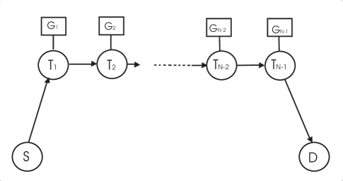
Figure 1: Multihop wireless communication system

III-B LCR and AFD of Multihop Transmissions

If the fading amplitude received at node $T_{i}$, $\alpha_{i}(t)$, is a time-correlated (due to mobility of $T_{i-1}$ and/or $T_{i}$) Rayleigh random process, distributed according to (1) at any given moment $t$, with mean power

$$\hat{\Omega}_{i}=E\{\alpha_{i}^{2}(t)\}\,,$$ (42)

then the $i$-th element of the product in (41)

$$X_{i}(t)=\alpha_{i}(t)G_{i-1}$$ (43)

is again a time-correlated Rayleigh random process, distributed according to (1), with mean power

$$\Omega_{i}=\hat{\Omega}_{i}\,G_{i-1}^{2}\,.$$ (44)

Comparing (8) and (41), we realize that the total fading amplitude at the destination station $D$ (i.e., the received desired signal without the AWGN) is described as the $N*$Rayleigh random process $Y(t)=\alpha(t)$, whose average LCR and AFD are determined in the previous Section.

Based on the system model from Fig. 1, if all stations are assumed mobile with maximum Doppler frequency shifts $f_{mS},f_{mD}$ , $f_{mi}(1\leq i\leq N-1)$ for source $S$, destination $D$ and relays, respectively, then for the $i$-th hop

$$f_{i}^{2}=f_{m(i-1)}^{2}+f_{mi}^{2}$$ (45)

with $f_{m0}=f_{mS}$ and $f_{mN}=f_{mD}$, and

$$\sum_{i=1}^{N}f_{i}^{2}=f_{mS}^{2}+2\sum_{i=1}^{N-1}f_{mi}^{2}+f_{mD}^{2}\,.$$ (46)

Using (II), (20) and (21), it is now straightforward to obtain the exact expressions for the average LCR and the AFD of the multihop Rayleigh fading channel, as follows

$$N_{\alpha}(\alpha)=\frac{2^{N-\frac{1}{2}}\sqrt{\pi}\alpha}{\Phi}$$ (47)

$$\times \int_{x_{1}=0}^{\infty}\cdots\int_{x_{N-1}=0}^{\infty}\left[\Omega_{N}f_{N}^{2}+\alpha^{2}\left(\prod_{i=1}^{N-1}\frac{1}{x_{i}^{2}}\right)\sum_{i=1}^{N-1}\frac{\Omega_{i}f_{i}^{2}}{x_{i}^{2}}\right]^{1/2}$$

$$\times \,\exp\left[-\left(\frac{\alpha^{2}}{\Omega_{N}}\prod_{i=1}^{N-1}\frac{1}{x_{i}^{2}}+\sum_{i=1}^{N-1}\frac{x_{i}^{2}}{\Omega_{i}}\right)\right]dx_{1}\cdots dx_{N-1}$$

and

$$T_{\alpha}(\alpha)=\frac{1}{N_{\alpha}(\alpha)}\,G_{1,N+1}^{N,1}\left[\frac{\alpha^{2}}{\Phi}\Bigg{|}\begin{array}[]{cc}\qquad 1\\ \underbrace{1,1,\cdots,1}_{N},0\end{array}\right],$$ (48)

respectively, where $f_{i}^{2}$ is given by (45) and $\Phi$ is given by (19).

It must be noted here that, for $N=2$, (47) is transformed into a single integral of the form

$$N_{\alpha}(\alpha)=\frac{4\sqrt{\pi}\alpha}{\sqrt{2}\Omega_{1}\Omega_{2}}\qquad\qquad\qquad\qquad\qquad\qquad\qquad\quad$$

$$\times\int_{0}^{\infty}\sqrt{\Omega_{2}f_{2}^{2}+\Omega_{1}f_{1}^{2}\frac{\alpha^{2}}{x^{4}}}\,\exp\left[-\left(\frac{\alpha^{2}}{x^{2}\Omega_{2}}+\frac{x^{2}}{\Omega_{1}}\right)\right]dx,$$ (49)

which, after changing integration variable $x$ with new variable $t$ according $x=\alpha/t$, reduces to the known result [13, Eq. (17)].

By combining (46) with (II-A) and (46) with (II-A), we also obtain approximate solutions for the average LCR and AFD of the multihop Rayleigh fading channel as

$$N_{\alpha}(\alpha)\approx\left[\frac{1}{N}\left(f_{mS}^{2}+2\sum_{i=1}^{N-1}f_{mi}^{2}+f_{mD}^{2}\right)\right]^{1/2}\qquad$$

$$\times\frac{(2\pi)^{N/2}\alpha}{\Phi^{1/2}}\exp\left(-N\frac{\alpha^{2/N}}{\Phi^{1/N}}\right)$$ (50)

and

$$T_{\alpha}(\alpha)\approx\left[\frac{1}{N}\left(f_{mS}^{2}+2\sum_{i=1}^{N-1}f_{mi}^{2}+f_{mD}^{2}\right)\right]^{-1/2}\qquad\qquad\quad$$

$$\times\frac{\Phi^{1/2}}{(2\pi)^{N/2}}\frac{1}{\alpha}\,\,G_{1,N+1}^{N,1}\left[\frac{\alpha^{2}}{\Phi}\Bigg{|}\begin{array}[]{cc}\qquad 1\\ \underbrace{1,1,\cdots,1}_{N},0\end{array}\right]\exp\left(N\frac{\alpha^{2/N}}{\Phi^{1/N}}\right),$$

(52)

respectively, where $\Phi$ is given by (19).

We see that (III-B) and (III-B) approximate the average LCR and AFD of the total fading amplitude for arbitrary power of the fading amplitudes $\hat{\Omega}_{i}$, arbitrary relay gains $G_{i}$ and arbitrary maximal Doppler shifts for the nodes $f_{mi}$.

It must be noted here that, for $N=2$, (III-B) is an efficient closed-form alternative to the corresponding one given by [13, Eq. (17)] for the dual-hop case. Furthermore, as it will be shown in the next section, the proposed approximation is highly accurate.

III-C Special Cases

If we assume that $i$) all stations are mobile and induce same maximal Doppler shifts (i.e., $f_{mS}=f_{mi}=f_{mD}=f_{m}$), $ii$) the fading amplitudes in all hops have equal powers (i.e., $\hat{\Omega}_{i}=\hat{\Omega}$), then (III-B) reduces to

$$N_{\alpha}(\alpha)\approx\sqrt{2}f_{m}\frac{(2\pi)^{N/2}\alpha}{\Phi^{1/2}}\,\exp\left(-N\frac{\alpha^{2/N}}{\Phi^{1/N}}\right)\,,$$ (53)

where, according to (19), $\Phi=\hat{\Omega}^{N}\,\prod_{i=1}^{N-1}G_{i}^{2}$.

If we assume that $i$) the destination station is fixed (i.e., $f_{mD}=0$) but all other stations are mobile inducing same maximal Doppler shifts (i.e., $f_{mS}=f_{mi}=f_{m}$), and $ii$) the fading amplitudes in all hops have equal powers (i.e., $\hat{\Omega}_{i}=\hat{\Omega}$), then (III-B) reduces to

$$N_{\alpha}(\alpha)\approx f_{m}\left(\frac{2N-1}{N}\right)^{1/2}\frac{(2\pi)^{N/2}\alpha}{\Phi^{1/2}}\exp\left(-N\frac{\alpha^{2/N}}{\Phi^{1/N}}\right)\,,$$

(54)

where again $\Phi=\hat{\Omega}^{N}\,\prod_{i=1}^{N-1}G_{i}^{2}$.

IV Numerical Results and Discussion

In this Section, we provide some illustrative examples for the average LCR and AFD of the fading gain process of the received desired signal at the destination of a multihop non-regenerative relay transmission system from Fig. 1. The numeric examples obtained from the derived approximate solutions are validated by extensive Monte-Carlo simulations over the system model described in Section III .

Based on the system model from Fig. 1, we considered a multihop transmission system consisted of a source terminal $S$, 4 fixed-gain relays, and a destination terminal $D$. The destination $D$ has fixed position, whereas the source and all relays are mobile and induce same maximal Doppler shift $f_{m}$.

The fixed-gain relays are assumed semi-blind with gains in Rayleigh fading channel calculated according to [2, Eq. (15)] and [11, Eq. (19)]

$$G_{i,sb}^{2}=\frac{1}{\hat{\Omega}_{i}}\,\exp\left(\frac{1}{\bar{\gamma}_{i}}\right)\,\Gamma\left(0,\frac{1}{\bar{\gamma}_{i}}\right),$$ (55)

where $\bar{\gamma}_{i}=\hat{\Omega}_{i}/W_{0,j}$ is the mean SNR on the $i$-th hop, and $\Gamma(\cdot,\cdot)$ is the incomplete Gamma function. Relay gain calculated according to (55) assures mean power consumption equal to that of a CSI-assisted relay, whose gain inverts the fading effect of the previous hop while limiting the output power at moments with deep fading.

Depending on the stations’ mobility, we used two different 2D isotropic scattering models for the Rayleigh radio channel on each hop of the multihop transmission system. For the fixed-to-mobile channel (hop), we used the classic Jakes channel model [16]-[17]. For the mobile-to-mobile channel (hop), we used the Akki and Habber’s channel model [18]-[19]. The Monte-Carlo simulations of the latter were realized by using the sum-of-sinusoids method proposed in [25]-[26].

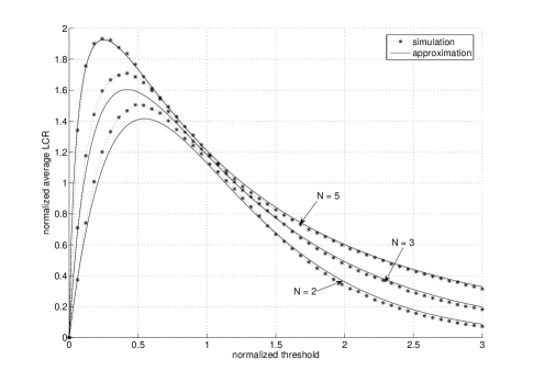
Figure 2: Average level crossing rate, when $\hat{\gamma}_{1}=\hat{\gamma}_{2}=\hat{\gamma}_{3}=\hat{\gamma}_{4}=\hat{\gamma}_{5}=\hat{\gamma}=5$ dB

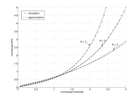
Figure 3: Average fade duration, when $\hat{\gamma}_{1}=\hat{\gamma}_{2}=\hat{\gamma}_{3}=\hat{\gamma}_{4}=\hat{\gamma}_{5}=\hat{\gamma}=5$ dB

Each presented figure depicts the received signal’s normalized LCR ($N_{\alpha}/f_{m}$) or normalized AFD ($T_{\alpha}f_{m}$) versus the normalized threshold ($\alpha/\sqrt{\hat{\Omega}}$) at 3 different nodes along the multihop transmission system: at relay $T_{2}$ (curve denoted by $N=2$), at relay $T_{3}$ (curve denoted by $N=3$) and at the destination $D$ (curve denoted by $N=5$). Note that, when applying the considered scenarios in (III-B) or (III-C), $\alpha$ and $\hat{\Omega}$ appear together as $\alpha/\sqrt{\hat{\Omega}}$.

Figs. 2-5 assume equal power of the fading amplitudes in all hops $\hat{\Omega}_{i}=\hat{\Omega}$, and equal variance of the AWGN $W_{0,i}=W_{0}$. Thus, $\bar{\gamma}_{i}=\bar{\gamma}$, $G_{i,sb}=G_{sb}$ for $1\leq i\leq 5$, so the mean of Rayleigh random process $X_{i}(t)=\alpha_{i}(t)G_{i-1,sb}$ is calculated as

$$\Omega_{i}=\exp\left(\frac{1}{\bar{\gamma}}\right)\,\Gamma\left(0,\frac{1}{\bar{\gamma}}\right)=\Omega,\quad 2\leq i\leq 5,$$ (56)

whereas $\Omega_{1}=\hat{\Omega}$ is selected independently from the AWGN, since $G_{0}=1$. In this case,

$$\Phi=\hat{\Omega}\,\exp\left(\frac{N-1}{\bar{\gamma}}\right)\,\left[\Gamma\left(0,\frac{1}{\bar{\gamma}}\right)\right]^{N-1}\,.$$ (57)

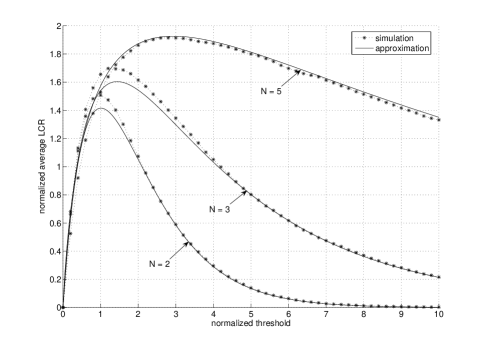
Figure 4: Average level crossing rate, when $\hat{\gamma}_{1}=\hat{\gamma}_{2}=\hat{\gamma}_{3}=\hat{\gamma}_{4}=\hat{\gamma}_{5}=\hat{\gamma}=20$ dB

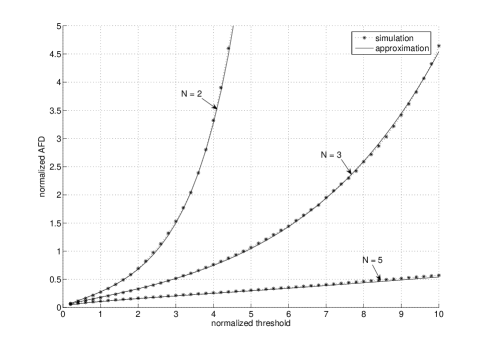
Figure 5: Average fade duration, when $\hat{\gamma}_{1}=\hat{\gamma}_{2}=\hat{\gamma}_{3}=\hat{\gamma}_{4}=\hat{\gamma}_{5}=\hat{\gamma}=20$ dB

Figs. 6-7 assume equal powers of the fading amplitudes in all hops $\hat{\Omega}_{i}=\hat{\Omega}$, and unequal variances of the AWGN $W_{0,i}$. Thus, the mean of Rayleigh random process $X_{i}(t)=\alpha_{i}(t)G_{i-1,sb}$ is calculated as

$$\Omega_{i}=\exp\left(\frac{1}{\bar{\gamma}_{i-1}}\right)\,\Gamma\left(0,\frac{1}{\bar{\gamma}_{i-1}}\right),\quad 2\leq i\leq 5,$$ (58)

whereas $\Omega_{1}=\hat{\Omega}$ is arbitrarily chosen. In this case,

$$\Phi=\hat{\Omega}\,\exp\left(\sum_{i=1}^{N-1}\frac{1}{\bar{\gamma}_{i}}\right)\,\prod_{i=1}^{N-1}\Gamma\left(0,\frac{1}{\bar{\gamma}_{i}}\right)\,.$$ (59)

All comparative curves show an excellent match between the approximate solution and the Monte-Carlo simulation for the considered scenarios.

The LCR curves, presented in Figs. 2, 4 and 6, manifest a behavior of a typical fading channel, since the average LCR increases with the threshold until some maximum, and then decreases. The maximized LCR and the maximizing threshold depend on number of hops and per hop SNRs $\bar{\gamma}_{i}$. The AFD, presented in Figs. 3, 5 and 7, also manifests a typical fading channel behavior, since AFD continuously increases with the threshold.

Regardless on the per hop SNRs, for some specified threshold, the $N*$Rayleigh fading signal typically remains less time in fading with the increase of $N$ (Figs. 3, 5, and 7), whereas its LCR increases (Figs. 2, 4, and 6). These differences are more pronounced with the increase of the per hop SNRs. Similarly, for some specified threshold, the LCR increases with the per hop SNR, whereas its AFD decreases. Namely, for the considered range of values for the $N$ and per hop SNR, $\Phi$ increases with respect to both of those parameters, yielding to those observations.

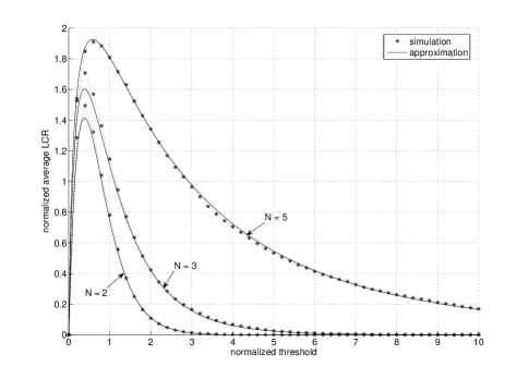
Figure 6: Average level crossing rate, when $\hat{\gamma}_{1}=0$ dB, $\hat{\gamma}_{2}=10$ dB, $\hat{\gamma}_{3}=15$ dB, $\hat{\gamma}_{4}=15$ dB, $\hat{\gamma}_{5}=20$ dB

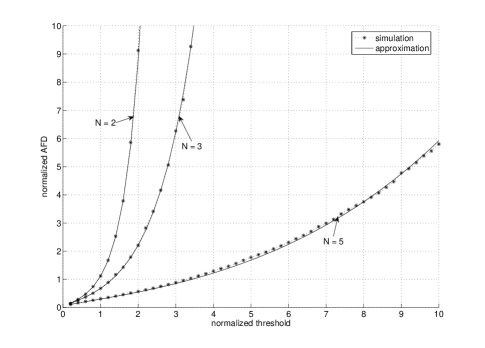
Figure 7: Average fade duration, when $\hat{\gamma}_{1}=0$ dB, $\hat{\gamma}_{2}=10$ dB, $\hat{\gamma}_{3}=15$ dB, $\hat{\gamma}_{4}=15$ dB, $\hat{\gamma}_{5}=20$ dB

V Conclusions

In this paper, motivated by the fact that the multihop AF Rayleigh fading channel is a cascaded one, we present a novel and general analytical framework for the exact evaluation of important second order statistical parameters, as the LCR and the AFD of this channel. Moreover, we present simple and efficient closed-form approximations for the aforementioned parameters, using the multivariate Laplace approximation theorem. The accuracy of the presented mathematical analysis and the tightness of the proposed closed-form approximations, were shown by numerical examples and extensive Monte-Carlo simulations. The material presented in this paper can be efficiently used in determining the packet length selection, power and bandwidth allocation over multiple hops, and maximum delay/latency requirement [12][29], or determining the delay spread of frequency-selective multihop channels [30]. Finally, it could be useful in the study of the second order statistics of the cooperative diversity systems.

Appendix A Laplace Approximation Theorem

Let $D$ be a possibly unbounded domain in the multidimensional space $R^{n}$, $u$ and $h$ be real-valued multivariate functions of $\mathbf{x}=[x_{1},...,x_{n}]$, and $\lambda$ is a real parameter. Consider the integral

$$J(\lambda)=\int_{\textbf{x}\in D}u(\textbf{x})\exp(-\lambda h(\textbf{x}))d\textbf{x}.$$ (A.1)

If $i$) the integral $J(\lambda)$ converges absolutely for all $\lambda\leq\lambda_{0}$, $ii$) function $h$ has an absolute minimum $\tilde{\mathbf{x}}=[\tilde{x}_{1},\cdots,\tilde{x}_{n}]$ at an interior point of $D$ (this is turn implies that $\tilde{\mathbf{x}}$ is a critical point of $h$, i.e., $\nabla h(\tilde{\mathbf{x}})=0$), and $iii$) the Hessian matrix

$$\mathbf{A} = \left[\left(\frac{\partial^{2}h}{\partial x_{i}\partial x_{j}}\right)\Bigg{|}_{\mathbf{x}=\mathbf{\tilde{x}}}\right]$$ (A.6)

$$= \left[\begin{array}[]{cccc}\frac{\partial^{2}h(\mathbf{\tilde{x}})}{\partial x_{1}^{2}}&\frac{\partial^{2}h(\mathbf{\tilde{x}})}{\partial x_{1}\partial x_{2}}&\cdots&\frac{\partial^{2}h(\mathbf{\tilde{x}})}{\partial x_{1}\partial x_{n}}\\ \frac{\partial^{2}h(\mathbf{\tilde{x}})}{\partial x_{2}\partial x_{1}}&\frac{\partial^{2}h(\mathbf{\tilde{x}})}{\partial x_{2}^{2}}&\cdots&\frac{\partial^{2}h(\mathbf{\tilde{x}})}{\partial x_{2}\partial x_{n}}\\ .&.&\cdots&.\\ \frac{\partial^{2}h(\mathbf{\tilde{x}})}{\partial x_{n}\partial x_{1}}&\frac{\partial^{2}h(\mathbf{\tilde{x}})}{\partial x_{n}\partial x_{2}}&\cdots&\frac{\partial^{2}h(\mathbf{\tilde{x}})}{\partial x_{n}^{2}}\\ \end{array}\right]$$

is positive definite, then, for large $\lambda$,

$$J(\lambda)\approx\left(\frac{2\pi}{\lambda}\right)^{n/2}\frac{u(\tilde{\mathbf{x}})}{\sqrt{\det(\mathbf{A})}}\exp(-\lambda h(\tilde{\mathbf{x}})),$$ (A.7)

where $\det(\cdot)$ represents the matrix determinant. The Laplace approximation theorem was originally proven by Hsu [23] for $\lambda\rightarrow\infty$. It was observed in [24] that in many cases of interest the Laplace approximation performs very well even in sub-asymptotic cases where $\lambda$ remains small.

References

• [1] J. N. Laneman, D. N. C. Tse, and G. W. Wornell, β€œCooperative Diversity in Wireless Networks: Efficient Protocols and Outage Behavior,” IEEE Trans. Inform. Theory, vol. 50, no. 12, pp. 3062-3080, Dec. 2004.
• [2] M. O. Hasna, and M. S. Alouini, β€œA performance study of dual-hop transmissions with fixed gain relays,” IEEE Trans. Wireless Commun., vo. 3, no. 6, pp. 1963-1968, Nov. 2004.
• [3] J. N. Laneman, and G. W. Wornell, β€œDistributed Space-Time Coded Protocols for Exploiting Cooperative Diversity in Wireless Networks,” IEEE Trans. Inform. Theory, vol. 49, no. 10, pp. 2415-2525, Oct. 2003.
• [4] M. O. Hasna, and M. S. Alouini, β€œEnd-to-end performance of transmission systems with relays over Rayleigh fading channels,” IEEE Trans. Wireless Commun., vol. 2, no. 6, pp. 1126-1131, Nov. 2003.
• [5] N. C. Beaulieu, and J. Hu, β€œA closed-form expression for the outage probability of decode-and-forward relaying in dissimilar Rayleigh fading channels,” IEEE Commun. Lett., vol. 10, no. 12, pp. 813-815, Dec. 2006.
• [6] I. -H. Lee, and D. Kim, β€œSymbol error probabilities for general cooperative links,” IEEE Trans. Wireless Commun., vol. 4, no. 3, pp. 1264-1273, May 2005.
• [7] K. S. Gomadam, and S. A. Jafar, β€œImpact of mobility on cooperative communication,” Proc. IEEE WCNC 2006
• [8] H. Mheidat, and M. Uysal, β€œNon-Coherent and Mismatched-Coherent Receivers for Distributed STBCs with Amplify-and-Forward Relaying”, IEEE Trans. Wireless Commun., vol. 6, no. 11, pp. 4060-4070, Nov. 2007.
• [9] M. O. Hasna, and M. S. Alouini, β€œOutage probability of multi-hop transmission over Nakagami fading channels,” IEEE Commun. Lett., vol. 7, no. 5, pp. 216-218, May 2003.
• [10] G. K. Karagiannidis, β€œPerformance bounds of multihop wireless communications with blind relays over generalized fading channels,” IEEE Trans. Wireless Commun., vol. 5, no. 3, pp. 498-503, March 2006.
• [11] G. K. Karagiannidis, T. Tsiftsis, and R. K. Malik, β€œBounds for multihop relayed communications in Nakagami-m fading,” IEEE Trans. Commun., vol. 54, no. 1, Jan. 2006.
• [12] L. Yang, M. O. Hasna, and M.-S. Alouini, β€œAverage Outage Duration of Multihop Communication Systems With Regenerative Relays,” IEEE Trans. Wireless Commun., vol. 4, no. 4, pp. 1366-1371, July 2005
• [13] C.S. Patel, G.L. Stuber and T.G. Pratt, β€œStatistical Properties of Amplify and Forward Relay Fading Channels,” IEEE Trans. Veh. Tech., vo. 55, no. 1, Jan. 2006
• [14] C. Iskander and P. Mathiopoulos, β€œAnalytical level crossing rates and average fade durations for diversity techniques in Nakagami fading channels,” IEEE Trans. on Commun., vol. COM-50, no. 8, pp. 1301-1309, Aug. 2002
• [15] X. Dong and N. C. Beaulieu, β€œAverage level crossing rate and average fade duration of selection diversity,” IEEE Commun. Lett., vol. 5, no. 10, pp. 396 398, Oct. 2001.
• [16] W. C. Jakes, Microwave Mobile Communications, Piscataway, NJ: IEEE Press, 1994.
• [17] G. L. Stuber, Principles of Mobile Communications, Boston: Kluwer Academic Publishers, 1996.
• [18] A. S. Akki and F. Haber, β€œA Statistical Model for Mobile-To-Mobile Land Communication Channel,” IEEE Trans. Veh. Technol., vol. VT-35, no. 1, pp. 2-7, Feb. 1986.
• [19] A.S. Akki, β€œStatistical Properties of Mobile-to-Mobile Land Communication Channels,” IEEE Trans. Veh. Tech., vol. 43, no. 4, pp. 826-831, Nov. 1994
• [20] G. K. Karagiannidis, N. C. Sagias, and P. T. Mathiopoulos, β€œN*Nakagami: A Novel Stochastic Model for Cascaded Fading Channels,” IEEE Trans. Commun., vol. 55, no. 8, pp. Aug. 2007
• [21] I. S. Gradshteyn and I.M. Ryzhik, Table of Integrals, Series, and Products, 6th ed. New York: Academic, 2000.
• [22] R. Wong, Asymptotic Approximations of Integrals, SIAM: Society for Industrial and Applied Mathematics, New edition, 2001.
• [23] L. C. Hsu, β€œA Theorem on the Asymptotic Behavior of a Multiple Integral,” Duke Mathematical Journal, 1948, pp. 623-632.
• [24] R. Butler and A. T. A. Wood, β€œLaplace Approximations for Hypergeometric Functions of Matrix Argument,” The Annals of Statistics, vol. 30, pp. 1155-1177, 2001.
• [25] C.S. Patel, G.L. St ber, and T.G. Pratt, β€œSimulation of Rayleigh-Faded Mobile-to-Mobile Communication Channels,” IEEE Trans. Commun., vol. 53, no. 11, pp. 1876-1884, Nov. 2005
• [26] A.G. Zajic and G.L. Stuber, β€œA New Simulation Model for Mobile-to-Mobile Rayleigh Fading Channels,” Proc. IEEE WNCN 2006
• [27] M. Abramowitz and I. A. Stegun, Handbook of Mathematical Functions with Formulas, Graphs, and Mathematical Tables, 9th ed. New York: Dover, 1970
• [28] V. S. Adamchik and O. I. Marichev, β€œThe algorithm for calculating integrals of hypergeometric type functions and its realization in REDUCE system,” Proc. Int. Conf. Symbolic and Algebraic Comput., Tokyo, Japan, 1990, pp. 212-224.
• [29] J. Lai and N. B. Mandayam, β€œMinimum duration outages in Rayleigh fading channels,” IEEE Trans. Commun., vol. 49, pp. 1755-1761, Oct. 2001.
• [30] K. Witrisal, Y.-H. Kim, and R. Prasad, β€œA new method to measure parameters of frequency-selective radio channels using power measurements,” IEEE Trans. Commun., vol. 49, pp. 1788-1800, Oct. 2001.