Level Crossing Rate and Average Fade Duration
of the Double Nakagami-$m$ Random Process
and Application in MIMO Keyhole Fading Channels

Abstract

We present novel exact expressions and accurate closed-form approximations for the level crossing rate (LCR) and the average fade duration (AFD) of the double Nakagami-$m$ random process. These results are then used to study the second order statistics of multiple input multiple output (MIMO) keyhole fading channels with space-time block coding. Numerical and computer simulation examples validate the accuracy of the presented mathematical analysis and show the tightness of the proposed approximations.

I Introduction

Recently, special attention has been given to the so-called “multiplicative” fading models. The double Rayleigh (i.e., Rayleigh*Rayleigh) channel fading model has been found to be suitable when both transmitter and receiver are moving [1]. Moreover, it has also been recently used for keyhole channel modeling of multiple-input multiple-output (MIMO) systems [2]-[3]. Its extension, the double Nakagami-$m$ (i.e., Nakagami-$m$*Nakagami-$m$) fading model, has been considered in [4], where the fading between each pair of transmit and receive antennas in presence of the “keyhole” is characterized as Nakagami-$m$ fading. However, all the above works describe and utilize only the first order statistical properties of these “multiplicative” fading models, such as the outage and the error probabilities. But, knowledge of the second order statistics for above fading models are equally important, and are applicable, for example, in modeling and design of the multihop communications systems [5].

In this letter, we focus on the second order statistics of the double Nakagami-$m$ random process, for which we determine exact and approximate analytical solutions for its level crossing rate (LCR) and average fade duration (AFD). Then we apply these results to study the second order statistics of the keyhole channels applicable to MIMO systems with space-time block coding (STBC), operating in specific rich-scattering environments. Note that although this work assumes independence among the channels, similar analysis can be used to derive LCR and AFD in correlated keyhole channels [9].

II On the second order statistics of the double Nakagami-$m$ random process

Let the double Nakagami-$m$ random process be defined as

$$Z(t)=X(t)Y(t)\,,$$ (1)

where $X(t)$ and $Y(t)$ are a pair of independent Nakagami-$m$ distributed RVs with probability distribution functions (PDFs)

$$f_{X}(x)=\left(\frac{m_{X}}{\Omega_{X}}\right)^{m_{X}}\frac{2x^{2m_{X}-1}}{\Gamma(m_{X})}\exp\left(-\frac{m_{X}x^{2}}{\Omega_{X}}\right)$$ (2)

and

$$f_{Y}(y)=\left(\frac{m_{Y}}{\Omega_{Y}}\right)^{m_{Y}}\frac{2y^{2m_{Y}-1}}{\Gamma(m_{Y})}\exp\left(-\frac{m_{Y}y^{2}}{\Omega_{Y}}\right)\,,$$ (3)

where $\Omega_{X}=E[X^{2}]$, $\Omega_{Y}=E[Y^{2}]$, and $m_{X}$ and $m_{Y}$ are the fading severity parameters, where $E[\cdot]$ means expectation.

If $X(t)$ and $Y(t)$ are signal envelopes in some scattering radio channel exposed to the Doppler effect due to stations’ relative mobility, then $X(t)$ and $Y(t)$ are time-correlated random processes. Considering a fixed-to-mobile channel, each scattered component of $X(t)$ and $Y(t)$ has some resulting Doppler spectra with maximum Doppler frequency shift $f_{mx}$ and $f_{my}$, respectively. It was shown in [6] that, under such conditions, the envelopes time derivatives $\dot{X}$ and $\dot{Y}$ are independent from their respective envelopes, while following zero-mean Gaussian PDFs with respective variances

$$\sigma_{\dot{X}}^{2}=(\pi f_{mx})^{2}\Omega_{X}/m_{X},\quad\sigma_{\dot{Y}}^{2}=(\pi f_{my})^{2}\Omega_{Y}/m_{Y}\,.$$ (4)

II-A Second order statistics

The LCR of $Z$ at threshold $z$ is defined as the rate at which the random process crosses level $z$ in the negative direction. To extract LCR, we need to determine the joint PDF of $Z$ and $\dot{Z}$, $f_{Z\dot{Z}}(z,\dot{z})$, and apply the Rice’s formula

$$N_{Z}(z)=\int_{0}^{\infty}\dot{z}f_{Z\dot{Z}}(\dot{z},z)d\dot{z}\,.$$ (5)

The above expression can be rewritten as

$$N_{Z}(z)=\int_{0}^{\infty}\left(\int_{0}^{\infty}\dot{z}f_{\dot{Z}|ZX}(\dot{z}|z,x)d\dot{z}\right)f_{Z|X}(z|x)f_{X}(x)dx$$ (6)

where $f_{\dot{Z}|ZX}(\cdot,\cdot,\cdot)$ is the conditional PDF of $\dot{Z}$ conditioned on $Z$ and $X$. This conditional PDF can be determined by finding the time derivative of both sides of (1),

$$\dot{Z}=Y\dot{X}+X\dot{Y}=\frac{Z}{X}\dot{X}+X\dot{Y}\,,$$ (7)

from which it is easily seen that, for fixed $Z=z$ and $X=x$, the time derivative $\dot{Z}$ is a zero-mean Gaussian RV with variance $\sigma_{\dot{Z}|ZX}^{2}=z^{2}\sigma_{\dot{X}}^{2}/x^{2}+x^{2}\sigma_{\dot{Y}}^{2}$. Now, the bracketed integral in (6) can be solved as

$$\int_{0}^{\infty}\dot{z}f_{\dot{Z}|ZX}(\dot{z}|z,x)d\dot{z}=\frac{\sigma_{\dot{Z}|ZX}}{\sqrt{2\pi}}\,.$$ (8)

The conditional PDF of $Z$ for some fixed $X=x$, $f_{Z|X}(z|x)$, is determined by simple transformation of RVs, $f_{Z|X}(z|x)=f_{Y}(z/x)/x$. Substituting (8) into (6), after some algebraic manipulations, we obtain the exact solution for the LCR

$$N_{Z}(z)=\frac{1}{\sqrt{2\pi}}\frac{4z^{2m_{Y}-1}\;\sigma_{\dot{Y}}}{\Gamma(m_{X})\Gamma(m_{Y})}\left(\frac{m_{X}}{\Omega_{X}}\right)^{m_{X}}\left(\frac{m_{Y}}{\Omega_{Y}}\right)^{m_{Y}}\quad$$

$$\times\int_{0}^{\infty}\sqrt{1+\frac{z^{2}}{x^{4}}\left(\frac{\sigma_{\dot{X}}}{\sigma_{\dot{Y}}}\right)^{2}}x^{2(m_{X}-m_{Y})}\;e^{-\big{(}\frac{m_{X}x^{2}}{\Omega_{X}}+\frac{m_{Y}z^{2}}{\Omega_{Y}x^{2}}\big{)}}dx$$ (9)

The above integral can be evaluated numerically with desired accuracy (e.g. by using some common software such as Mathematica). Alternatively, one can apply the Laplace approximation to obtain a highly accurate closed-form solution of (II-A) - as presented in the following subsection.

The AFD of $Z$ at threshold $z$ is defined as the average time that the double Nakagami-$m$ random process remains below level $z$ after crossing that level in the downward direction,

$$T_{Z}(z)=\frac{F_{Z}(z)}{N_{Z}(z)}\,,$$ (10)

where $F_{Z}(z)$ denotes the CDF of $Z$, which was derived only recently in closed-form for $N$*Nakagami random process [7]. For the double Nakagami random process, it attains the form

$$F_{Z}(z)=\frac{1}{\Gamma(m_{X})\Gamma(m_{Y})}\,G_{1,3}^{2,1}\left[z^{2}\frac{m_{X}m_{Y}}{\Omega_{X}\Omega_{Y}}\Bigg{|}\begin{array}[]{cc}\qquad 1\\ m_{X},m_{Y},0\end{array}\right],$$ (11)

where $\Gamma(\cdot)$ and $G[\cdot]$ are gamma and Meijer’s $G$ functions.

II-B Laplace approximation

Using [8], the Laplace type integral can be approximated as

$$\int_{0}^{\infty}g(x)\;e^{-\lambda f(x)}dx\approx\sqrt{\frac{2\pi}{\lambda}}\frac{g(x_{0})}{\sqrt{f^{{}^{\prime\prime}}(x_{0})}}\,e^{-\lambda f(x_{0})}\,,$$ (12)

when the real valued parameter $\lambda$ is very large (i.e., $\lambda\to\infty$). In (12), $f(x)$ and $g(x)$ are real-valued functions of $x$ and $x_{0}$ is the point at which $f(x)$ has an absolute minimum (known as the interior critical point of $f(x)$). Note, that $f^{\prime\prime}(x)$ denotes the second derivative of $f(x)$ with respect to $x$. It was observed that above approximation is very accurate even for small values of $\lambda$ [8]. Comparing (12) and (II-A), these functions are set as

$$f(x)=\frac{m_{X}x^{2}}{\Omega_{X}}+\frac{m_{Y}}{\Omega_{Y}}\left(\frac{z}{x}\right)^{2}-\ln(x^{2(m_{X}-m_{Y})})\,,$$ (13)

$$g(x)=\sqrt{1+\frac{z^{2}}{x^{4}}\left(\frac{\sigma_{\dot{X}}}{\sigma_{\dot{Y}}}\right)^{2}}\,,$$ (14)

whereas the second derivative of the former is $f^{{}^{\prime\prime}}(x)=2m_{X}/\Omega_{X}+6(m_{Y}z^{2})/(\Omega_{Y}x^{4})+2(m_{X}-m_{Y})/x^{2}$ and $\lambda=1$. The critical point of $f(x)$ is determining as the value of $x$ for which $\partial f/\partial x=0$, i.e.,

$$x_{0}=\Big{[}\frac{1}{2m_{X}\Omega_{Y}}\Big{(}\Omega_{X}\Omega_{Y}(m_{X}-m_{Y})\qquad\qquad\qquad\quad$$

$$+\sqrt{\Omega_{X}^{2}\Omega_{Y}^{2}(m_{X}-m_{Y})^{2}+4m_{X}m_{Y}\Omega_{X}\Omega_{Y}z^{2}}\,\Big{)}\Big{]}^{\frac{1}{2}}.$$ (15)

Using (13)-(II-B), the approximate closed-form solutions for the LCR and the AFD are respectively obtained as

$$N_{Z}(z)\approx\frac{4z^{2m_{Y}-1}\;\sigma_{\dot{Y}}}{\Gamma(m_{X})\Gamma(m_{Y})}\qquad\qquad\qquad\qquad\qquad\qquad\quad$$

$$\times\left(\frac{m_{X}}{\Omega_{X}}\right)^{m_{X}}\left(\frac{m_{Y}}{\Omega_{Y}}\right)^{m_{Y}}\frac{g(x_{0})}{\sqrt{f^{{}^{\prime\prime}}(x_{0})}}\,e^{-f(x_{0})}\,,\quad$$ (16)

$$T_{Z}(z)\approx\frac{1}{4z^{2m_{Y}-1}\;\sigma_{\dot{Y}}}\left(\frac{\Omega_{X}}{m_{X}}\right)^{m_{X}}\left(\frac{\Omega_{Y}}{m_{Y}}\right)^{m_{Y}}\qquad\qquad$$

$$\times\frac{\sqrt{f^{{}^{\prime\prime}}(x_{0})}\;\;e^{f(x_{0})}}{g(x_{0})}\;\;G_{1,3}^{2,1}\left[z^{2}\frac{m_{X}m_{Y}}{\Omega_{X}\Omega_{Y}}\Bigg{|}\begin{array}[]{cc}\qquad 1\\ m_{X},\,m_{Y},\,0\end{array}\right].$$ (19)

Although substitution of $f(x_{0})$, $f^{{}^{\prime\prime}}(x_{0})$ and $g(x_{0})$ into (II-B) and (II-B) is omitted for brevity, we emphasize that the threshold $z$ appears only as the ratio $z^{2}/((\Omega_{X}/m_{X})(\Omega_{Y}/m_{Y}))$.

III MIMO STBC Communication over Keyhole Fading Channels

Potentials of MIMO communications systems are not always achievable even for a fully uncorrelated transmit and receive channels, which is attributed to the rank deficiency of the MIMO channels known as the keyhole or pinhole effect [2]. The existence of the keyhole MIMO channels has been proposed and demonstrated through physical examples, where, although spatially uncorrelated, these channels still have a single degree of freedom [2]-[3]. Under the keyhole effect, the entries of the channel matrix, $\mathbf{H}$, follow statistics described as a product of two independent single-path gains.

III-A The MIMO keyhole channel model

From [4], the complex path gain of baseband equivalent signal transmitted over the channel between the $i$-th transmit and the $j$-th receive antenna at arbitrary moment $t$ is expressed as $1\leq i\leq M,1\leq j\leq N$

$$h_{ij}(t)=\alpha_{i}(t)\beta_{j}(t)e^{j(\phi_{i}(t)+\psi_{j}(t))},$$ (20)

where $\left\{\alpha_{i}(t)e^{j\phi_{i}(t)}\right\}_{i=1}^{M}$ are the complex path gains introduced by the rich-scattered channel from the $i$-th transmitting antenna to the “keyhole”, and $\left\{\beta_{j}(t)e^{j\psi_{j}(t)}\right\}_{j=1}^{N}$ are the complex path gains introduced by the rich-scattered channel from the “keyhole” to the $j$-th receiving antenna. Phases $\left\{\phi_{i}(t)\right\}_{i=1}^{M}$ and $\left\{\psi_{j}(t)\right\}_{j=1}^{N}$ are independent and uniformly distributed over $[0,2\pi)$. The amplitudes $\left\{\alpha_{i}(t)\right\}_{i=1}^{M}$ and $\left\{\beta_{j}(t)\right\}_{j=1}^{N}$ are i.i.d. Nakagami-$m$ RVs. The fading severity parameters of $\alpha_{i}(t)$ are equal to $m_{T}$, whereas $\Omega_{T}=E[\alpha_{i}^{2}]$ for all $i$. Similarly, the fading severity parameters of $\beta_{j}(t)$ are equal to $m_{R}$, whereas $\Omega_{R}=E[\beta_{j}^{2}]$ for all $j$. Assuming mobility of both the transmitter and the receiver with respect to the “keyhole”, all channel gains are time-correlated random processes with maximum Doppler shifts $f_{\alpha_{i}}=f_{\alpha}$ and $f_{\beta_{i}}=f_{\beta}$, respectively. Under such conditions, the time derivatives $\dot{\alpha}_{i}$ and $\dot{\beta}_{j}$ are independent from $\alpha_{i}$ and $\beta_{j}$, respectively, and both follow zero-mean Gaussian PDFs with variances given by (4), $\sigma_{\dot{\alpha}_{i}}^{2}=(\pi f_{\alpha})^{2}\Omega_{T}/m_{T}$, $1\leq i\leq M$ and $\sigma_{\dot{\beta}_{j}}^{2}=(\pi f_{\beta})^{2}\Omega_{R}/m_{R}$, $1\leq j\leq N$.

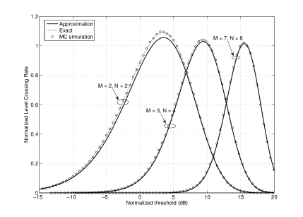
Figure 1: Normalized LCR for various number of transmit and receive antennas

III-B Orthogonal space-time block coding and decoding

The orthogonal space time block encoding and decoding (signal combining) transform a MIMO fading channel into an equivalent single-input-single-output (SISO) fading channel with a path gain of the squared Frobenius norm of the MIMO channel matrix $\mathbf{H}(t)=\left[h_{ij}(t)\right]_{M\times N}$ [4],

$$||\mathbf{H}(t)||_{F}^{2}=\sum_{i=1}^{M}\sum_{j=1}^{N}|h_{ij}(t)|^{2}=\left(\sum_{i=1}^{M}\alpha_{i}^{2}(t)\right)\left(\sum_{j=1}^{N}\beta_{j}^{2}(t)\right)$$ (21)

at arbitrary moment $t$. After space-time block decoding, the instantaneous output signal-to-noise ratio (SNR) per symbol is given by

$$\gamma(t)=\frac{\bar{\gamma}}{MR}||\mathbf{H}(t)||_{F}^{2}\,,$$ (22)

where $\bar{\gamma}=E_{s}/N_{0}$ is the average SNR per receive antenna, and $R$ is the rate of the STBC.

III-C Second order statistics of output SNR

We introduce the auxiliary random process $Z(t)$ defined by

$$Z(t)=\sqrt{||\mathbf{H}(t)||_{F}^{2}}=X(t)Y(t)\,,$$ (23)

where $X(t)=\sqrt{\sum_{i=1}^{M}\alpha_{i}^{2}(t)}$ and $Y(t)=\sqrt{\sum_{j=1}^{N}\beta_{j}^{2}(t)}$ are again Nakagami-$m$ distributed with PDFs given by (2) and (3), respectively, with $m_{X}=Mm_{T}$, $\Omega_{X}=M\Omega_{T}$, $m_{Y}=Nm_{R}$ and $\Omega_{Y}=N\Omega_{R}$. The time derivatives $\dot{X}$ and $\dot{Y}$ are independent from $X$ and $Y$, respectively, and both follow the zero-mean Gaussian PDF with variances given by (4), $\sigma_{\dot{X}}^{2}=\sigma_{\dot{\alpha}_{i}}^{2}=(\pi f_{\alpha})^{2}\Omega_{T}/m_{T}$ and $\sigma_{\dot{Y}}^{2}=\sigma_{\dot{\beta}_{j}}^{2}=(\pi f_{\beta})^{2}\Omega_{R}/m_{R}$.

Hence, the random process $Z(t)$, defined by (23), is a double Nakagami-$m$ process for which we can apply the analytical framework of Section II to determine its exact and approximate LCR and AFD by using (II-A), (11), (II-B) and (II-B). With above in mind, the LCR and the AOD of instantaneous output SNR, given by (22), are respectively determined as

$$N_{\gamma}(\gamma) = N_{Z}(\sqrt{\gamma MR/\bar{\gamma}})\,,$$ (24)

$$T_{\gamma}(\gamma) = T_{Z}(\sqrt{\gamma MR/\bar{\gamma}})\,.$$ (25)

IV Numerical Results

We present several numerical examples for the LCR and the AFD of the STBC MIMO communications system operating over a keyhole fading channel. The mobile transmitter and the mobile receiver are assumed to introduce same maximum Doppler shifts due to same relative speeds with respect to the “keyhole”, yielding $f_{\alpha}=f_{\beta}=f_{m}$.

Figs. 1 and 2 depict the normalized LCR ($N_{\gamma}/f_{m}$) and normalized AFD ($T_{\gamma}\,f_{m}$) of the instantaneous output SNR vs. normalized SNR threshold. The normalized SNR threshold ($x$-axis) is calculated as $10\log[\gamma\,MR/(\bar{\gamma}(\Omega_{T}/m_{T})(\Omega_{R}/m_{R}))]$. The results are obtained for three different pairs of number of transmit and receive antennas $(M,N)$, appearing as curve parameters. For each pair $(M,N)$, the three comparative curves on both figures indicate excellent match between the exact and the approximate solutions for the two statistical parameters, both of which are validated by Monte Carlo simulations.

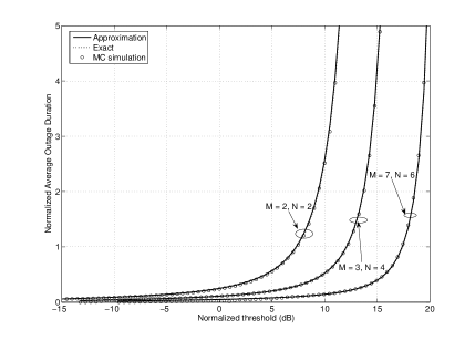
Figure 2: Normalized AOD for various number of transmit and receive antennas

References

• [1] J. B. Andersen, β€œStatistical distributions in mobile communications using multiple scattering,” Proc. Gen. Assem. Int. Union of Radio Sci., Maastricht, The Netherlands, Aug. 2002.
• [2] D. Gesbert, H. Bolcskei, D. A. Gore, and A. J. Paulraj, β€œMimo wireless channels: Capacity and performance prediction,” Proc. GLOBECOM 2000, vol. 2, pp. 1083-1088
• [3] D. Chizhik, G. J. Foschini, M. J. Gans, and R. A. Valenzuela, β€œKeyholes, correlations, and capacities of multielement transmit and receive antennas,” IEEE Trans. Wireless Commun., vol. 1, no. 2, pp. 361-368, Apr. 2002
• [4] H. Shin and J. H. Lee, β€œPerformance analysis of space-time block codes over keyhole Nakagami-$m$ fading channels,” IEEE Trans. Veh. Technol., vol. 53, no. 2, pp. 351-362, Mar. 2004
• [5] Z. Hadzi-Velkov, N. Zlatanov, G. K. Karagiannidis, β€œOn the second order statistics of the multihop Rayleigh fading channel,” accepted for publication in the IEEE Transactions on Communications, 2008
• [6] M. D. Yacoub, J. E.V. Bautista, and L. G. de Rezende Guedes, β€œOn higher order statistics of the Nakagami-$m$ distribution,” IEEE Trans. Commun., vol. 48, No. 3, pp. 790-794, May 1999
• [7] G. K. Karagiannidis, N. C. Sagias, and P. T. Mathiopoulos, β€œN𝑁N*Nakagami: a novel stochastic model for cascaded fading fhannel,” IEEE Trans. Commun., vol. 55, No. 8, pp. 1453-1458, Aug. 2007
• [8] R. Wong, Asymptotic Approximations of Integrals, SIAM: Society for Industrial and Applied Mathematics, New edition, 2001.
• [9] G. Levin, S. Loyka, β€œOn the Outage Capacity Distribution of Correlated Keyhole MIMO Channels”, IEEE Trans. on Inform. Theory, vol. 54, no.7, pp. 3232-3245, July 2008.