An Accurate Approximation to the Distribution of the Sum of Equally Correlated Nakagami-$m$ Envelopes and its Application in Equal Gain Diversity Receivers

Abstract

We present a novel and accurate approximation for the distribution of the sum of equally correlated Nakagami-$m$ variates. Ascertaining on this result we study the performance of Equal Gain Combining (EGC) receivers, operating over equally correlating fading channels. Numerical results and simulations show the accuracy of the proposed approximation and the validity of the mathematical analysis.

I Introduction

The knowledge of the statistics of the sums of multiple signals’s envelopes is important in the analytical performance evaluation, such as that of equal gain combining (EGC) systems. However, the evaluation of the probability distribution function (PDF) and the cumulative distribution function (CDF) of these sums can be rather cumbersome even for the statistically independent Nakagami-$m$ or Rayleigh fading channels [2]-[7]. An infinite series technique for computing the PDF of a sum of independent random variables (RVs) was derived in [2]. Applying this technique, the error rate performance of EGC systems under Nakagami fading was presented in [3], whereas, in [4], the problem was analyzed in frequency domain in terms of semi-analytical expressions with infinite integrals. Other two studies on EGC diversity in Nakagami fading that use numerical integration over Gil-Palaez single infinite integral and Hermite quadrature over double finite-infinite integral are presented in [5] and [6], respectively. Closed form solutions for some modulation schemes are also obtained for dual and triple diversity under Rayleigh fading [2], [5]. All above mentioned works assumed independent fading channels.

However, in real-life applications, fading among diversity branches is correlated, which renders the analytical analysis under correlated Nakagami fading with a particular practical interest. Since the joint PDF of multiple correlated fading branches is not known, the published results for EGC diversity in correlated fading channels deal primarily with the dual branch case [7]-[9], where error probabilities for binary and QAM signals over correlated Rayleigh channels are expressed in form of infinite series.

Only several papers address EGC in correlated fading with multiple order diversity. In [10], EGC performance was determined by approximating the moment generating function (MGF) of its output SNR, where the moments are determined exactly for exponentially correlated Nakagami channels in terms of multi-fold infinite series. A completely novel approach for performance analysis of diversity combiners in equally correlated fading channels was proposed in [11], where the equally correlated Rayleigh fading channels are transformed into a set of conditionally independent Rician RVs. Based on this technique, the authors in [12] derive the moments of the EGC output SNR in equally correlated Nakagami channels in terms of the Lauricella hypergeometric function, and then uses them to evaluate the EGC performance measures, such as outage probability (as infinite series) and error probability (using Gaussian quadrature with weights and abscissas computed by solving sets of nonlinear equations).

All of the above approaches yield to results that are somewhat complex, not expressed in closed form, and require computation of infinite series, all of which is attributed to the inherent intricacy of the exact sum statistics. This intricacy can be circumvented by searching for suitable highly accurate approximations for a sum of arbitrary number of Nakagami RVs. Various simple and accurate approximations to the PDF of sum of independent Rayleigh, Rice and Nakagami RVs are proposed in [13]-[15], which then are used for analytical EGC performance evaluation. [15] uses the moment matching method to arrive at the required approximation.

In this paper, we use the moment matching method to obtain highly accurate closed form PDF approximation for the sum of arbitrary number of non-identical equally correlated Nakagami RVs with arbitrary mean powers. We then apply this approximation to efficiently estimate the performance of EGC systems by avoiding many complex numerical calculations inherent for the methods in abovementioned previous works. Even approximate closed form expressions allow one to gain insight into system performance by considering, for example, large SNR or small SNR behaviors.

II An Accurate Approximation to the Sum of Equally Correlated Nakagami-$m$ Envelopes

Let $Z$ be a sum of $L$ non-identical equally correlated Nakagami-$m$ RVs, $Z_{1}$, $Z_{2}$, … , $Z_{L}$,

$$Z=\sum_{k=1}^{L}Z_{k},$$ (1)

The PDF of each envelope $Z_{k}$, $1\leq k\leq L$ is given by [1]

$$f_{Z_{k}}(z)=\left(\frac{m_{z}}{\Omega_{k}}\right)^{m_{z}}\frac{2z^{2m_{z}-1}}{\Gamma(m_{z})}\exp\left(-\frac{m_{z}}{\Omega_{k}}z^{2}\right),\qquad z\geq 0$$ (2)

having an arbitrary second moment $E[Z_{k}]=\Omega_{k}$, $1\leq k\leq L$, same fading parameter $m_{z}$ (assumed to be positive integer) and same envelope correlation coefficient between each pair of RVs

$$\rho_{Z}=\frac{{\rm{cov}}(Z_{i}^{2},Z_{j}^{2})}{\sqrt{{\rm{var}}(Z_{i}^{2}){\rm{var}}(Z_{j}^{2})}},\qquad i\neq j$$ (3)

where $E[\cdot]$, $\rm{cov}(\cdot,\cdot)$ and $\rm{var}(\cdot)$ denote expectation, covariance and variance, respectively.

We propose the unknown PDF of be approximated by the PDF of an equivalent RV defined as

$$R=\sqrt{\sum_{k=1}^{L}R_{k}^{2}},$$ (4)

where $R_{k}$, $1\leq k\leq L$, represent a different set of $L$ identical equally correlated Nakagami RVs with equal average powers, $E[R_{k}]=\Omega_{R}$, equal fading parameters $m_{R}$ and equal correlation coefficient $\rho_{R}$. Additionally, it is assumed that

$$\rho_{R}=\rho_{Z}=\rho\,.$$ (5)

Both the MGF and the PDF of $R^{2}$ had been determined in closed form as [16, Eqs. (42a) and (36)]

$$M_{R^{2}}(s)=E[e^{sR^{2}}]=\left(1-s\frac{\Omega_{R}(1+(L-1)\sqrt{\rho})}{m_{R}}\right)^{-m_{R}}$$

$$\times\left(1-s\frac{\Omega_{R}(1-\sqrt{\rho})}{m_{R}}\right)^{-m_{R}(L-1)}\,,\qquad$$ (6)

and

$$f_{R^{2}}(r)=\left(\frac{m_{R}}{\Omega_{R}}\right)^{m_{R}L}\qquad\qquad\qquad\qquad\qquad\qquad\qquad\quad$$

$$\times\,\frac{r^{m_{R}L-1}}{\Gamma(m_{R}L)(1-\sqrt{\rho})^{m_{R}(L-1)}(1+(L-1)\sqrt{\rho})^{m_{R}}}\qquad\quad$$

$$\times\,\exp\left(-\frac{m_{R}r}{(1-\sqrt{\rho})\Omega_{R}}\right)\qquad\qquad\qquad\qquad\qquad\qquad\quad$$

$$\times\,{}_{1}F_{1}\left(m_{R},m_{R}L,\frac{\sqrt{\rho}m_{R}Lr}{(1-\sqrt{\rho})(1+(L-1)\sqrt{\rho})\Omega_{R}}\right)\,,\qquad$$ (7)

respectively, where ${}_{1}F_{1}(\cdot,\cdot,\cdot)$ is the Kummer confluent hypergeometric function [17, Eq. (9.210)]. The PDF of $R$ is determined by simple transformation of RVs, $f_{R}(r)=2rf_{R^{2}}(r^{2})$, which yields to

$$f_{R}(r)=\left(\frac{m_{R}}{\Omega_{R}}\right)^{m_{R}L}\qquad\qquad\qquad\qquad\qquad\qquad\qquad\quad$$

$$\times\,\frac{2r^{2m_{R}L-1}}{\Gamma(m_{R}L)(1-\sqrt{\rho})^{m_{R}(L-1)}(1+(L-1)\sqrt{\rho})^{m_{R}}}\qquad\quad$$

$$\times\,\exp\left(-\frac{m_{R}r^{2}}{(1-\sqrt{\rho})\Omega_{R}}\right)\qquad\qquad\qquad\qquad\qquad\qquad\quad\,$$

$$\times\,{}_{1}F_{1}\left(m_{R},m_{R}L,\frac{\sqrt{\rho}m_{R}Lr^{2}}{(1-\sqrt{\rho})(1+(L-1)\sqrt{\rho})\Omega_{R}}\right)\,.\qquad$$ (8)

One now needs to determine $\Omega_{R}$ and $m_{R}$ so that (II) be an accurate approximation of the PDF of $Z$ defined by (1). For this, we apply the moment matching method by respectively matching the second and fourth moments of RVs $Z$ and $R$:

$$E[Z^{2}] \,=\, E[R^{2}]\,,$$ (9)

$$E[Z^{4}] \,=\, E[R^{4}]\,.$$ (10)

The second and the fourth moments of $R$ are determined straightforwardly by using the MGF (II) and applying the moment theorem, i.e.,

$$E[R^{2}] = \frac{dM_{R^{2}}(s)}{ds}\big{|}_{s=0}=L\Omega_{R}\,,$$ (11)

$$E[R^{4}] = \frac{d^{2}M_{R^{2}}(s)}{ds^{2}}\big{|}_{s=0}=\frac{L\Omega_{R}}{m_{R}}(1-\rho+L(m_{R}+\rho))\,.$$

The second and fourth moments of $Z$ are determined by applying the multinomial theorem and the results presented in [10, Eq. (21)], [12, Eq. (43)] and Appendix A, yielding

$$E[Z^{2}]=\sum_{k=1}^{L}\Omega_{k}+2\frac{\Gamma^{2}(m_{z}+1/2)}{m_{z}\Gamma^{2}(m_{z})}\left(\sum_{i=1}^{L}\sum_{j=i+1}^{L}\sqrt{\Omega_{i}\Omega_{j}}\right)$$

$$\times\,{}_{2}F_{1}\left(-\frac{1}{2},-\frac{1}{2};m_{z};\rho\right)\,,\qquad\qquad$$ (13)

and

$$E[Z^{4}] = \left(\frac{1-\sqrt{\rho}}{m_{z}}\right)^{2}\left[W(4)\sum_{k=1}^{L}\Omega_{k}^{2}+6W(2,2)\right.$$

$$\times \sum_{i=1}^{L}\sum_{j=i+1}^{L}\Omega_{i}\Omega_{j}+4W(3,1)\sum_{i=1}^{L}\sum_{j=i+1}^{L}\left(\sqrt{\Omega_{i}^{3}\Omega_{j}}\right.$$

$$+ \left.\sqrt{\Omega_{i}\Omega_{j}^{3}}\right)+12W(2,1,1)\sum_{m=1}^{L}\sum_{i=m+1}^{L}\sum_{j=i+1}^{L}$$

$$\left(\sqrt{\Omega_{m}^{2}\Omega_{i}\Omega_{j}}+\sqrt{\Omega_{m}\Omega_{i}^{2}\Omega_{j}}+\sqrt{\Omega_{m}\Omega_{i}\Omega_{j}^{2}}\right)+24$$

$$\times \left.W(1,1,1,1)\sum_{m=1}^{L}\sum_{n=m+1}^{L}\sum_{i=n+1}^{L}\sum_{j=i+1}^{L}\sqrt{\Omega_{m}\Omega_{n}\Omega_{i}\Omega_{j}}\right]$$

where

$$W(k_{1},\cdots,k_{N})=\left(\prod_{j=1}^{N}\frac{\Gamma(m_{z}+k_{j}/2)}{\Gamma(m_{z})}\right)\frac{1}{\Gamma(m_{z})}\qquad\qquad\,$$

$$\times\int_{0}^{\infty}u^{m_{z}-1}e^{-u}\prod_{j=1}^{N}{}_{1}F_{1}\left(-\frac{k_{j}}{2},m_{z};-\frac{u\sqrt{\rho}}{1-\sqrt{\rho}}\right)du\qquad\,$$ (15)

with ${}_{2}F_{1}\left(\cdot,\cdot;\cdot;\cdot\right)$ denoting the Gauss hypergeometric function [17, Eq. (9.100)]. Note that (II) and (II) are valid only if $m_{z}$ is positive integer [12]. Using [18, Vol. 4, Eq. (3.35.7(4))] and the Lauricella transformation to assure convergence [22, pp. 121], (II) is expressed in closed form as follows

$$W(k_{1},\cdots,k_{N})=\Big{(}\prod_{j=1}^{N}\frac{\Gamma(m_{z}+k_{j}/2)}{\Gamma(m_{z})}\Big{)}\Big{(}\frac{1-\sqrt{\rho}}{1+(N-1)\sqrt{\rho}}\Big{)}^{m_{z}}$$

$$\times\,F_{A}\left(m_{z};\,m_{z}+\frac{k_{1}}{2},\cdots,m_{z}+\frac{k_{N}}{2};\,m_{z},\cdots,m_{z};\right.\qquad\quad$$

$$\left.\frac{\sqrt{\rho}}{1+(N-1)\sqrt{\rho}},\cdots,\frac{\sqrt{\rho}}{1+(N-1)\sqrt{\rho}}\right)\,,\qquad\,$$ (16)

where $F_{A}(\cdots)$ denotes the Lauricella hypergeometric function of $N$ variables defined by [17, Eq. (9.19)]. Note that coefficients $W(4)$, $W(2,2)$, $W(3,1)$ and $W(2,1,1)$ can be expressed in terms of the more familiar hypergeometric functions as per (B.1), (B.2), (B.4) and (B.6), respectively.

Introducing (9) and (9) into (11) and (11), one obtains the needed parameters for the PDF approximation (II) of $Z$ in closed form as

$$\Omega_{R} = \frac{E[Z^{2}]}{L}\,,$$ (17)

$$m_{R} = \frac{1+(L-1)\rho}{L}\frac{(E[Z^{2}])^{2}}{E[Z^{4}]-(E[Z^{2}])^{2}}\,,$$ (18)

where $E[Z^{2}]$ and $E[Z^{4}]$ are respectively determined from (II) and (II). Note that the fading parameter $m_{R}$ is typically calculated to a positive real number.

II-A Special Case: Sum of Identical Equally Correlated Nakagami RVs

Let the equally correlated Nakagami RVs $Z_{k}$ ,$1\leq k\leq L$ have same second moments $E[Z_{k}^{2}]=\Omega_{Z}$ (equipowered branches), same fading parameter $m_{Z}$ (as positive integer) and same correlation coefficient $\rho$ between each pair of RVs. In this case, (II) and (II) are simplified by using (A.6) into

$$E[Z^{2}]=L\Omega_{Z}\left[1+\frac{(L-1)\Gamma^{2}(m_{z}+1/2)}{m_{z}\Gamma^{2}(m_{z})}\right.\qquad\qquad\qquad\quad$$

$$\times\,{}_{2}F_{1}\left(-\frac{1}{2},-\frac{1}{2};m_{z};\rho\right)\bigg{]}\,,\qquad\quad$$ (19)

$$E[Z^{4}]=\left(\frac{\Omega_{Z}(1-\sqrt{\rho})}{m_{z}}\right)^{2}\,\Big{[}L\,W(4)+3L(L-1)\,W(2,2)$$

$$+4\,L(L-1)\,W(3,1)+6L(L-1)(L-2)\,W(2,1,1)$$

$$+\,L(L-1)(L-2)(L-3)\,W(1,1,1,1)\Big{]}\,,\qquad\qquad\,\,\,$$ (20)

where the necessary coefficients $W(k_{1},k_{2},k_{3},k_{4})$ are again calculated by (II). The needed parameters for the PDF approximation (II) of $Z$ are obtained from (17) and (18).

III Application in the performance analysis of EGC receivers

We consider a typical $L$-branch EGC diversity receiver exposed to slow and flat Nakagami fading. The envelopes of the useful branch signals $Z_{k}$ are non-identical equally correlated Nakagami random processes with PDFs given by (2), whereas their respective phases are i.i.d. uniform random processes. Each branch is also corrupted by additive white Gaussian noise (AWGN) with power spectral density $N_{0}/2$, which is added to the useful branch signal. In the EGC receiver, the random phases of the branch signals are compensated (co-phased), equally weighted and then summed together to produce the decision variable.

The envelope of the composite useful signal, denoted by $Z$, is given by (1), whereas the composite noise power is given by $\sigma_{EGC}^{2}=LN_{0}/2$, resulting in the instantaneous output SNR given by

$$\gamma_{EGC}=\frac{Z^{2}}{2\sigma_{EGC}^{2}}=\frac{1}{LN_{0}}\left(\sum_{k=1}^{L}Z_{k}\right)^{2}=\left(\sum_{k=1}^{L}G_{k}\right)^{2}$$ (21)

where RVs $G_{k}=Z_{k}/\sqrt{LN_{0}}$, $1\leq k\leq L$, form a set of $L$ non-identical equally correlated Nakagami RVs with $E[G_{k}^{2}]=\bar{\gamma}_{k}/L$, same fading parameters $m_{z}$ and same correlation coefficient $\rho$ among the diversity branches. Note that $\bar{\gamma}_{k}=\Omega_{k}/N_{0}$ denotes the average SNR in the $k$-th branch.

Using the results from Section II, it is now possible to approximate PDF and MGF of (21) by (II) and (II), respectively, with $\Omega_{R}$ replaced by $\bar{\gamma}=\Omega_{R}/(LN_{0})$. These closed form approximations are then used to determine the outage probability and the error probability of $L$-branch EGC systems in correlated Nakagami fading with high accuracy.

III-A Outage Probability

The closed form approximation of the outage probability of the EGC receiver (i.e. the CDF of $\gamma_{EGC}$) at threshold $t$ is obtained by applying [18, Vol. 5, Eq. (2.1.3(1))] over (II) as

$$F_{\gamma_{EGC}}(t)\approx\Big{(}\frac{m_{R}t}{\bar{\gamma}(1+(L-1)\sqrt{\rho})}\Big{)}^{m_{R}}\Big{(}\frac{m_{R}t}{\bar{\gamma}(1-\sqrt{\rho})}\Big{)}^{m_{R}(L-1)}$$

$$\times\,\frac{1}{\Gamma(1+m_{R}L)}\,\,\Phi_{2}\Big{(}m_{R},\,m_{R}(L-1);\,1+m_{R}L;\qquad\qquad$$

$$-\frac{m_{R}t}{\bar{\gamma}(1+(L-1)\sqrt{\rho})},\,-\frac{m_{R}t}{\bar{\gamma}(1-\sqrt{\rho})}\Big{)}\,,\qquad$$ (22)

where $\Phi_{2}(\cdot,\cdot;\cdot;\cdot,\cdot)$ denotes the confluent hypergeometric function of two variables defined by [17, Eq. (9.261(2))].

III-B Average Error Probability

Comparing (1) and (4), it is obvious that the error performance of an EGC system can be approximated by the performance of an equivalent maximal ratio combining (MRC) system for which many closed form solutions exist. For example, [19] derives the error probabilities of $L$-branch MRC with coherent and non-coherent detection of binary signals in identical correlated Nakagami fading channels. Thus, the average bit error probabilities of the coherent BPSK system and non-coherent BFSK are respectively expressed as [19, Eq. (32)] and [19, Eq. (26)]

$$\bar{P}_{C-BPSK}=\frac{1}{2}-\sqrt{\frac{1}{\pi}}\frac{\Gamma(m_{R}L+1/2)}{\Gamma(m_{R}L)}\left[\frac{\bar{\gamma}(1-\sqrt{\rho})}{m_{R}+\bar{\gamma}(1-\sqrt{\rho})}\right]^{\frac{1}{2}}$$

$$\times\left[\frac{m_{R}}{m_{R}+\bar{\gamma}(1-\sqrt{\rho})}\right]^{m_{R}L}\left[\frac{1-\sqrt{\rho}}{1+(L-1)\sqrt{\rho}}\right]^{m_{R}}\qquad\qquad$$

$$\times\,F_{2}\left(m_{R}L+\frac{1}{2};1,m_{R};\frac{3}{2},m_{R}L;\frac{\bar{\gamma}(\sqrt{\rho}-1)}{m_{R}+\bar{\gamma}(1-\sqrt{\rho})}\right.,\qquad$$

$$\frac{m_{R}L\sqrt{\rho}}{(m_{R}+\bar{\gamma}(1-\sqrt{\rho}))(1+(L-1)\sqrt{\rho}}\bigg{)}\,,\qquad$$ (23)

and

$$\bar{P}_{NC-BFSK}=\frac{1}{2}\,M_{R^{2}}(s)\bigg{|}_{s=-\frac{1}{2}}\,.\qquad\qquad\qquad\qquad\quad$$ (24)

where $F_{2}(\cdot;\cdot,\cdot;\cdot,\cdot;\cdot,\cdot)$ is the Appell hypergeometric function (as the special case of Lauricella $F_{A}$ function of two variables) defined by [17, Eq. (9.180(2))].

IV Illustrative Examples and Discussion

In this Section, the proposed approximation for the sum of arbitrary number of non-identical equally correlated Nakagami channels is validated by Monte-Carlo simulations. The simulation of correlated Nakagami random signals is realized by using the method proposed in [21, Section VII].

In order to model the non-identical branch signals (i.e., unequal average branch powers and unequal average branch SNRs), we introduce exponentially decaying profile, modeled as

$$\Omega_{k}=\Omega_{1}\exp(-\delta(k-1)),\qquad 1\leq k\leq L,$$ (25)

where $\Omega_{1}$ is the average power of branch 1 ($k=1$) and $\delta$ is the decaying exponent. Note that $\delta=0$ denotes the case of identical branch signals (i.e., equal branch powers and equal average branch SNRs).

Fig. 1 illustrate the high accuracy of the proposed PDF approximation of RV (1) for a large variety of fading scenarios.

Figs. 2 and 3 illustrate the high accuracy of the equivalent BPSK MRC error probability (III-B) for evaluation of the approximated BPSK EGC error probability.

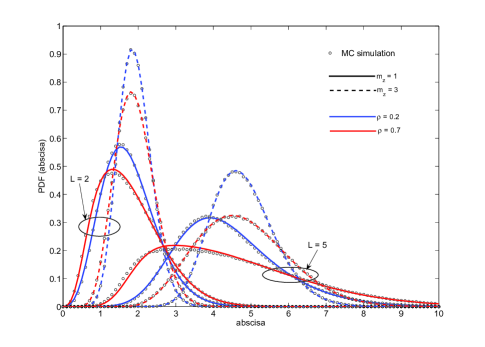
Figure 1: PDF approximation of a sum of $L$ identical equally correlated Nakagami RVs for $\Omega_{1}=1$ and $\delta=0$

Appendix A

In order to determine $E[Z^{2}]$ and $E[Z^{4}]$, we apply the multinomial theorem [20, Eq. (24.1.2)]. The second moment $E[Z^{2}]$ can be extracted straightforwardly. The fourth moment $E[Z^{4}]$, after using [4, Eq. (43)] and performing some mathematical manipulations, can be transformed to

$$E[Z^{4}] = \left(\frac{1-\sqrt{\rho}}{m_{z}}\right)^{2}\bigg{[}W(4)\sum_{k=1}^{L}\Omega_{k}^{2}+6W(2,2)$$

$$\times \sum_{i=1}^{L}\sum_{j=i+1}^{L}\Omega_{i}\Omega_{j}+4W(3,1)\sum_{i=1}^{L}\sum_{j=i+1}^{L}\sqrt{\Omega_{i}^{3}\Omega_{j}}$$

$$+ 4W(1,3)\sum_{i=1}^{L}\sum_{j=i+1}^{L}\sqrt{\Omega_{i}\Omega_{j}^{3}}$$

$$+ 12W(2,1,1)\sum_{m=1}^{L}\sum_{i=m+1}^{L}\sum_{j=i+1}^{L}\sqrt{\Omega_{m}^{2}\Omega_{i}\Omega_{j}}$$

$$+ 12W(1,2,1)\sum_{m=1}^{L}\sum_{i=m+1}^{L}\sum_{j=i+1}^{L}\sqrt{\Omega_{m}\Omega_{i}^{2}\Omega_{j}}$$

$$+ 12W(1,1,2)\sum_{m=1}^{L}\sum_{i=m+1}^{L}\sum_{j=i+1}^{L}\sqrt{\Omega_{m}\Omega_{i}\Omega_{j}^{2}}$$

$$+24W(1,1,1,1)\sum_{m=1}^{L}\sum_{n=m+1}^{L}\sum_{i=n+1}^{L}\sum_{j=i+1}^{L}\sqrt{\Omega_{n}\Omega_{m}\Omega_{i}\Omega_{j}}\bigg{]}$$ (A.1)

It is obvious from (II) that $W(3,1)=W(1,3)$ and $W(2,1,1)=W(1,2,1)=W(1,1,2)$, which directly yields to the result given by (II).

Appendix B

Using identities given by [20, Eqs. (13.6.9) and (22.3.9)], ${}_{1}F_{1}(0,m_{z},-au)=1$, ${}_{1}F_{1}(-1,m_{z},-au)=1+au/m_{z}$ and ${}_{1}F_{1}(-2,m_{z},-au)=1+2au/m_{z}+(au)^{2}/(m_{z}(1+m_{z}))$, one directly obtains

$$W(4)=\left(\frac{\Gamma(m_{z}+2)}{\Gamma(m_{z})}\right)\frac{1}{\Gamma(m_{z})}\qquad\qquad\qquad\qquad\qquad$$

$$\times\int_{0}^{\infty}u^{m_{z}-1}e^{-u}{}_{1}F_{1}\left(-2,m_{z};-au\right)du\qquad$$

$$=m_{z}(1+m_{z})(1+a)^{2}\,,\qquad\qquad\qquad\qquad\qquad$$ (B.1)

$$W(2,2)=\left(\frac{\Gamma(m_{z}+1)}{\Gamma(m_{z})}\right)^{2}\frac{1}{\Gamma(m_{z})}\qquad\qquad\qquad\qquad\quad$$

$$\times\int_{0}^{\infty}u^{m_{z}-1}e^{-u}\big{[}{}_{1}F_{1}\left(-1,m_{z};-au\right)\big{]}^{2}du\qquad\quad$$

$$=a^{2}m_{z}+m_{z}^{2}(1+a)^{2}\,,\qquad\qquad\qquad\qquad\qquad$$ (B.2)

where $a=\sqrt{\rho}/(1-\sqrt{\rho})>0$. Using [17, Eqs. (9.212 (1)) and (7.622 (1))], it is possible to obtain the following identity

$$J(m,a,p,q)=\frac{1}{\Gamma(m)}\int_{0}^{\infty}u^{m-1}e^{-u}{}_{1}F_{1}\left(-\frac{p}{2},m;-au\right)$$

$$\times{}_{1}F_{1}\left(-\frac{q}{2},m;-au\right)du=(1+a)^{\frac{p}{2}}\left(\frac{1+2a}{1+a}\right)^{\frac{q}{2}}$$

$$\times\,{}_{2}F_{1}\left(m+\frac{p}{2};-\frac{q}{2};m,-\frac{a^{2}}{1+2a}\right)\,,\qquad$$ (B.3)

resulting into

$$W(3,1)=\left(\frac{\Gamma(m_{z}+3/2)}{\Gamma(m_{z})}\frac{\Gamma(m_{z}+1/2)}{\Gamma(m_{z})}\right)\frac{1}{\Gamma(m_{z})}\qquad\qquad\quad$$

$$\int_{0}^{\infty}u^{m_{z}-1}e^{-u}{}_{1}F_{1}\left(-\frac{3}{2},m_{z};-au\right){}_{1}F_{1}\left(-\frac{1}{2},m_{z};-au\right)du$$

$$=\frac{\Gamma(m_{z}+3/2)}{\Gamma(m_{z})}\frac{\Gamma(m_{z}+1/2)}{\Gamma(m_{z})}J(m_{z},a,3,1)\,.\qquad\qquad$$ (B.4)

Using [17, Eq. (9.212 (3)), pp. 1023] and after some simple algebra, one obtains the following

$$\left[{}_{1}F_{1}\left(-\frac{1}{2},m;-au\right)\right]^{2}\qquad\qquad\qquad\qquad\qquad\qquad\qquad\qquad\quad$$

$$=\left(\frac{m+1/2}{m}\right)^{2}\left[{}_{1}F_{1}\left(-\frac{1}{2},m+1;-au\right)\right]^{2}\qquad\qquad\qquad\qquad$$

$$+\frac{1}{4m^{2}}\left[{}_{1}F_{1}\left(\frac{1}{2},m+1;-au\right)\right]^{2}\qquad\qquad\qquad\qquad\qquad\qquad$$

$$-\frac{m+1/2}{m^{2}}{}_{1}F_{1}\left(\frac{1}{2},m+1;-au\right){}_{1}F_{1}\left(-\frac{1}{2},m+1;-au\right)\qquad$$

(B.5)

Thus,

$$W(2,1,1)=\left(\frac{\Gamma(m_{z}+1)}{\Gamma(m_{z})}\left(\frac{\Gamma(m_{z}+1/2)}{\Gamma(m_{z})}\right)^{2}\right)\frac{1}{\Gamma(m_{z})}\qquad\qquad$$

$$\int_{0}^{\infty}u^{m_{z}-1}e^{-u}{}_{1}F_{1}\left(-1,m_{z};-au\right)\left[{}_{1}F_{1}\left(-\frac{1}{2},m_{z};-au\right)\right]^{2}du\quad$$

$$=m_{z}\left(\frac{\Gamma(m_{z}+1/2)}{\Gamma(m_{z})}\right)^{2}\bigg{[}J(m_{z},a,1,1)+\frac{a(m_{z}+1/2)^{2}}{m_{z}^{2}}\qquad$$

$$\times\,J(m_{z}+1,a,1,1)+\frac{a}{4m_{z}^{2}}J(m_{z}+1,a,-1,-1)\qquad\,\,$$

$$-\frac{a(m_{z}+1/2)}{m_{z}^{2}}J(m_{z}+1,a,-1,1)\bigg{]}\qquad$$

(B.6)

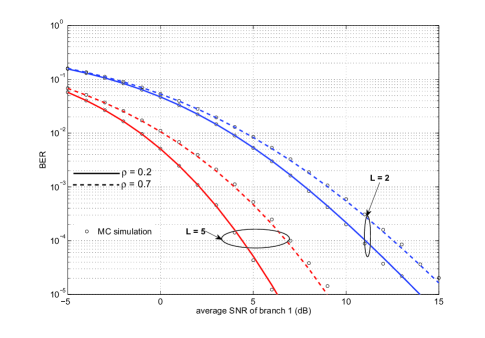
Figure 2: BER of equivalent MRC BPSK system for $m_{z}=2$ and $\delta=0$

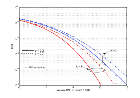
Figure 3: BER of equivalent MRC BPSK system for $m_{z}=2$ and $\delta=0.5$

References

• [1] M. Nakagami, ”The m-distribution A general formula of intensity distribution of rapid fading,” Statistical Methods in Radio Wave Propagation, W. G. Hoffman, Ed. Oxford, U.K.: Pergamon, 1960.
• [2] N. C. Beaulieu, ”An Infinite Series for the Computation of the Complementary Probability Distribution Function of a Sum of Independent Random Variables and Its Application to the Sum of Rayleigh Random Variables,” IEEE Transactions on Communications, vol. 38, no. 9, September 1990, pp. 1463 1474
• [3] N. C. Beaulieu and A. A. Abu-Dayya, ”Analysis of Equal Gain Diversity on Nakagami Fading Channels,” IEEE Transactions on Communications, vol. 39, no. 2, February 1991, pp. 225 234
• [4] A. Annamalai, C. Tellambura and Vijay K. Bhargava, ”Equal-gain diversity receiver performance in wireless channels,” IEEE Transactions on Communications, vol. 48, no. 10, October 2000, pp. 1732 1745
• [5] Q. T. Zhang, ”Probability of error for equal-gain combiners over Rayleigh channels: Some closed-form solutions,” IEEE Trans. Commun., vol. 45, no. 3, pp. 270 273, Mar. 1997.
• [6] M.-S. Alouini and M.K. Simon, ”Performance analysis of coherent equal gain combining over Nakagami-$m$ fading channels,” IEEE Trans. Vehic. Technol., vol. 50, pp. 1449-1463, Nov. 2001.
• [7] R. Mallik, M. Win, and J. Winters, ”Performance of dual-diversity predetection EGC in correlated Rayleigh fading with unequal branch SNRs,” IEEE Trans. Commun., vol. 50, no. 7, pp. 1041 1044, Jul. 2002.
• [8] C.-D. Iskander and P. T. Mathiopoulos, ”Performance of M-QAM with coherent equal gain combining in correlated Nakagami-$m$ fading,” IEE Electron. Lett., vol. 39, pp. 141 142, Jan. 2003.
• [9] G. K. Karagiannidis, D. A. Zogas, and S. A. Kotsopoulos, ”BER performance of dual predetection EGC in correlative Nakagami-$m$ fading,” IEEE Trans. Commun., vol. 52, no. 1, pp. 50 53, Jan. 2004.
• [10] G. K. Karagiannidis, ”Moments-based approach to the performance analysis of equal gain diversity in Nakagami-$m$ fading,” IEEE Transactions on Communications, vol. 52, no. 5, May 2004, pp. 685 690
• [11] Y. Chen and C. Tellambura, ”Performance analysis of l-branch equal gain combiners in equally-correlated Rayleigh fading channels,” IEEE Commun. Lett., vol. 8, no. 3, pp. 150 152, Mar. 2004.
• [12] Y. Chen and C. Tellambura, ”Moment Analysis of the Equal Gain Combiner Output in Equally Correlated Fading Channels,” IEEE Trans. Veh. Tech., vol. 54, No. 6, Nov. 2005, pp. 1971-1979
• [13] J. Hu and N. C. Beaulieu, ”Accurate closed-form approximations to Ricean sum distributions and densities,” IEEE Commun. Lett., vol. 9, no. 2, pp. 133 135, Feb. 2005.
• [14] J. Hu and N. C. Beaulieu, ”Accurate closed-form approximations for the error rate and outage of equal gain combining diversity in Nakagami fading channels,” Proc. ICC 2006, No. 1, June 2006, pp. 5129 - 5136
• [15] J. C. S. Santos Filho and M. D. Yacoub, ”Nakagami-$m$ approximation to the sum of M non-identical independent Nakagami-$m$ variates,” Electron. Lett., vol. 40, no. 15, pp. 951 952, July 2004.
• [16] M. S. Simon and M. S. Alouini, ”A unified approach to the performance analysis of digital communication over generalized fading channels”, Proceedings of IEEE, vol. 86, no. 9, pp. 1860-1877, Sept. 1998
• [17] I. S. Gradshteyn and I.M. Ryzhik, Table of Integrals, Series, and Products, 5th ed. New York: Academic, 1994.
• [18] A. P. Prudnikov, Yu. A. Brychkov and O. I. Marichev, Integrals and Series, Vol. 4 and Vol. 5. New York: Gordon and Breach, 1992.
• [19] V. A. Aalo, ”Performance of Maximal-Ration Diversity Systems in a Correlated Nakagami-Fading Environment”, IEEE Trans. Commun., Vol. 43, No. 8, pp. 2360-2369, Aug. 1995
• [20] M. Abramovitz and I. A. Stegun, Handbook of Mathematical Functions with Formulas, Graphs, and Mathematical Tables, 9th ed. New York: Dover, 1972.
• [21] Q. T. Zhang, ”A decomposition technique for efficient generation of correlated Nakagami fading channels”, IEEE Journal of Selected Areas of Commun., vol. 18, no. 11, pp. 2385-2392, Nov. 2000
• [22] H. Exton, Multiple Hypergeometric Functions and Applications, G. M. Bell, Ed. Sussex, U.K.: Ellis Horwood, 1976