Augmented space recursion code and application in simple binary metallic alloy

Abstract

We present here an optimized and parallelized version of the augmented space recursion code for the calculation of the electronic and magnetic properties of bulk disordered alloys, surfaces and interfaces, either flat, corrugated or rough, and random networks. Applications have been made to bulk disordered alloys to benchmark our code.

:

1 Introduction

The aim of this communication is to present and describe a computational package to handle first-principles density functional (DFT) based studies of electronic structure of systems without long-ranged lattice translational symmetry. Bulk disordered alloys and surfaces and interfaces which are either flat, corrugated or rough fall under this category which our formalism should be able to take care of. The aim is also to go beyond the usual mean-field approaches like the coherent potential approximation (CPA) and be able to take into account configuration fluctuations of the local environment. Lack of lattice translational symmetry means that the standard reciprocal space techniques based on the powerful Bloch theorem can no longer be applicable and we shall depend on alternative techniques based purely on real space approaches. Our formalism will be a marriage of three distinct methods which have been individually applied extensively : namely, the recursion method (RM) of Haydock et.al. [1]-[2], the augmented space method proposed by one of us [3]-[4] (ASR) and the tight-binding, linear muffin-tin orbitals method (TB-LMTO) [5]. The last mentioned provides us with a DFT self-consistent sparse representation of the Hamiltonian in a real-space minimal basis $\{|{\vec{R}}_{n}L\rangle\}$ which spans the Hilbert space ${\cal H}$. Here ${\vec{R}}_{n}$ labels the sites where the ion-cores sit and $L=(\ell m\sigma)$ are the angular momentum indexes. For a disordered system the matrix elements of the Hamiltonian representation in this basis are random. This representation is then taken over by the ASR to generate a modified Hamiltonian representation in the outer product space of ${\cal H}$ and the space ${\cal C}$ of configuration fluctuations of the random parameters. This modified Hamiltonian in the augmented space ${\cal H}\otimes{\cal C}$ represents a collection of all possible Hamiltonians for all possible configurations of Hamiltonian representations. Once this is done the RM allows us to obtain the matrix elements of the Green functions related to the Kohn-Sham equation for the electronic states. The augmented space theorem (AST) [6] relates a specific matrix element of the Green function in the augmented space ${\cal H}\otimes{\cal C}$ to the configuration averaged Green functions. The RM is a purely real-space based technique, and therefore as applicable to a bulk system as one with surfaces, interfaces or extended defects. In the following we shall describe each of the points raised above in some detail.

2 Tight-binding linear muffin-tin orbitals method

The TB-LMTO has been described in great detail earlier [5],[7]-[9]. We shall only quote here the main results which will be relevant for setting up the ASR programme. The starting point is the Kohn-Sham equation with the muffin-tin effective crystal potential. The basis chosen for representation of the wave-function are the muffin-tin orbitals $\{|{\vec{R}}_{n}L\rangle\}$ : If we expand the wave-function in terms of a linear combination of these muffin-tin orbitals and substitute the expansion in the Kohn-Sham equation we obtain the Korringa-Kohn-Rostocker (KKR) secular equation :

$$\det\parallel P_{{\vec{R}}_{n}L}(E)\delta_{{\vec{R}}_{n}{\vec{R}}_{m}}\delta_{LL^{\prime}}-S_{{\vec{R}}_{n}L,{\vec{R}}_{n}L^{\prime}}(\kappa)\parallel=0$$

Energy linearization gives the eigen-type LMTO secular equation:

$$\det\parallel E\delta_{{\vec{R}}_{n}{\vec{R}}_{m}}\delta_{LL^{\prime}}-H^{(2)}_{{\vec{R}}_{n}L,{\vec{R}}_{m}L^{\prime}}\parallel=0$$ (1)

where, the ‘second order’ Hamiltonian is given by :

$$\underline{\underline{H}}\/^{(2)}_{{\vec{R}}_{n},{\vec{R}}_{m}}=\underline{\underline{E}}\/_{\nu}\ \delta_{{\vec{R}}_{n}{\vec{R}}_{m}}+\underline{\underline{h}}\/_{{\vec{R}}_{n},{\vec{R}}_{m}}-\sum_{{\vec{R}}_{n}}\ \underline{\underline{h}}\/_{{\vec{R}}_{n},{\vec{R}}_{k}}\ \underline{\underline{o}}\/_{{\vec{R}}_{k}}\ \underline{\underline{h}}\/_{{\vec{R}}_{k},{\vec{R}}_{m}}$$ (2)

Note that each element is a matrix in the $L$ space. In the screened representation the structure matrix $\underline{\underline{S}}\/_{{\vec{R}}_{n}{\vec{R}}_{m}}$ is short-ranged and the Hamiltonian is sparse :

$$\underline{\underline{h}}\/_{{\vec{R}}_{n},{\vec{R}}_{m}}=(\underline{\underline{C}}\/_{{\vec{R}}_{n}}-\underline{\underline{E}}\/_{\nu})\ \delta_{{\vec{R}}_{n}{\vec{R}}_{m}}+\underline{\underline{\Delta}}\/^{1/2}_{{\vec{R}}_{n}}\ \underline{\underline{S}}\/_{{\vec{R}}_{n},{\vec{R}}_{m}}(0)\ \underline{\underline{\Delta}}\/^{1/2}_{{\vec{R}}_{m}}$$ (3)

The expansion energies $E_{\nu L}$ are chosen suitably by us at the center of the energy window of our interest and the potential parameters $\underline{\underline{C}}\/,\underline{\underline{\Delta}}\/$ and $\underline{\underline{o}}\/$ are diagonal in $L$ space and are self-consistently generated. The structure matrix $\underline{\underline{S}}\/$ is obtained from the geometry of the lattice. Note that the TB-LMTO basis is minimal and hence usually it is enough to take $\ell\leq 3$ and in a majority of cases one does not have to go beyond $\ell=2$

At this point we should comment on several possible generalizations : we have energy linearized the secular equation. In case we do not wish to do so, we can still deal with a energy dependent “Hamiltonian” or “secular matrix” $\underline{\underline{R}}\/(E)=\underline{\underline{P}}\/(E)-\underline{\underline{S}}\/(\kappa)$. This is the TB-KKR. The subsequent recursion becomes energy-dependent, however each recursion at each energy point can be parallely carried out for efficiency. Such energy dependent recursion has been carried out by us earlier [10]. The assumption (a posteriori shown after calculations) was that the recursion coefficients are weakly energy dependent, therefore recursion is carried out an equi-spaced “seed” points and the intermediate points found by interpolation. Further, if we allow for third-nearest neighbour sparsity in the Hamiltonian we could start with the real-space full-potential LMTO (RS-FPLMTO) of Eriksson et.al.[11].

3 The Recursion method

Whereas,the above formulation is general enough, we should stress on the fact that the Hamiltonian representation is an infinite matrix. Lack of lattice translation symmetry means that we are unable to symmetry reduce the dimensionality of the matrix to essentially $2\ell_{max}+1$. We therefore have to resort to techniques which allow us to deal with infinite matrices. The Recursion method was exactly such a technique introduced by Haydock et.al.[1]-[2] to obtain the Green functions associated with the secular equation. This would give us the density of states from which we may obtain properties like the Fermi energy, the charge and magnetization densities, the magnetic moment and the band energy. A recent generalization also gives us correlation functions associated with response functions [12]-[13].

The RM begins by recursively changing the basis through a three term recurrence relation :

$$|1\rangle = |{\vec{R}}_{i}L\rangle\qquad\mbox{and}\qquad|2\rangle={\bf H}\/^{(2)}|1\rangle-\alpha_{1}|1\rangle$$

$$|n+1\rangle = {\bf H}\/^{(2)}|n\rangle-\alpha_{n}|n\rangle-\beta^{2}_{n}|n-1\rangle\qquad\mbox{for}\quad n>1$$ (4)

Mutual orthogonality of this new basis gives :

$$\alpha_{n}=\frac{\langle n|{\bf H}\/^{(2)}|n\rangle}{\langle n|n\rangle}\quad\mbox{and}\quad\beta_{n}^{2}=\frac{\langle n+1|n+1\rangle}{\langle n|n\rangle}$$ (5)

To understand how the above equations are efficiently operationally coded on the computer, let us first describe the Hamiltonian as an operator H⁽²⁾. From Eqn.(2)

$${\bf H}\/^{(2)} = {\bf E}_{\nu}+{\bf h}-{\bf h}\ {\bf o}\ {\bf h}\quad\mbox{ and }\quad{\bf h}={\bf C}-{\bf E}_{\nu}+{\mathbf{\Delta}}^{1/2}\ {\bf S}\ {\mathbf{\Delta}}^{1/2}$$ (6)

Of these operators four are ‘diagonal’ : E_ν, C, ${\mathbf{\Delta}}^{1/2}$ and o. Their structure are all of the form : ${\mathbf{D}}=\sum_{i}\ \underline{\underline{D}}\/_{i}\ |R_{i}\rangle\langle R_{i}|=\sum_{i}\underline{\underline{D}}\/_{i}{\cal{P}}_{i}$. While the structure matrix is off-diagonal : ${\mathbf{S}}=\sum_{(ij)}\underline{\underline{S}}\/_{{\vec{R}}_{i}{\vec{R}}_{j}}\left(|{\vec{R}}_{i}\rangle\langle{\vec{R}}_{j}|+|{\vec{R}}_{j}\rangle\langle{\vec{R}}_{i}|\right)=\sum_{(ij)}\underline{\underline{S}}\/_{{\vec{R}}_{i}{\vec{R}}_{j}}{\cal{T}}_{ij}$.

If we represent a Hilbert space ‘vector’ $|n\rangle$ by a matrix as shown below :

$$|n\rangle\Longrightarrow\left(\begin{array}[]{cccc}n_{11}&n_{12}&\ldots&n_{1L}\\ n_{21}&n_{22}&\ldots&n_{2L}\\ &\vdots&\vdots&\\ n_{p1}&n_{p2}&\ldots&n_{pL}\\ &\vdots&\vdots&\\ \end{array}\right)\Longrightarrow\left(\begin{array}[]{c}\underline{n}\/_{1}\\ \underline{n}\/_{2}\\ \vdots\\ \underline{n}\/_{p}\\ \vdots\end{array}\right)$$

The action of the diagonal operators D is rather simple:

1. One by one choose non-zero rows $\underline{n}\/_{i}$ of $|n\rangle$

2. Multiply $\underline{\underline{D}}\/_{i}\ \underline{n}\/^{T}_{i}$ and add this to the $i$-th row of a new $|n^{\prime}\rangle$.

3. Repeat this for all non-zero rows of $|n\rangle$. Finally $|n^{\prime}\rangle={\bf D}|n\rangle$

The action of the off-diagonal operator S is more complicated as it has the information of the underlying lattice or network embedded in it. The first step would be to prepare the “neighbour map” (NM). The NM is a matrix $\underline{\underline{N}}\/=N_{ij}$ where $N_{ij}$ is the $j$-th neighbour of the $i$-th site on the lattice or network. We have first to number the lattice/network points by integers. The near neighbour vectors point in different directions, while numbering this directionality has to be carefully recorded, since the structure matrix between ${\vec{R}}_{n}$ and ${\vec{R}}_{m}$ will depend upon the direction of ${\vec{R}}_{n}-{\vec{R}}_{m}$. In figure 1 we show the geometry of a bulk square lattice, a square lattice with a plane surface (100), one with a corrugated surface (110) and a network with four local bonds.

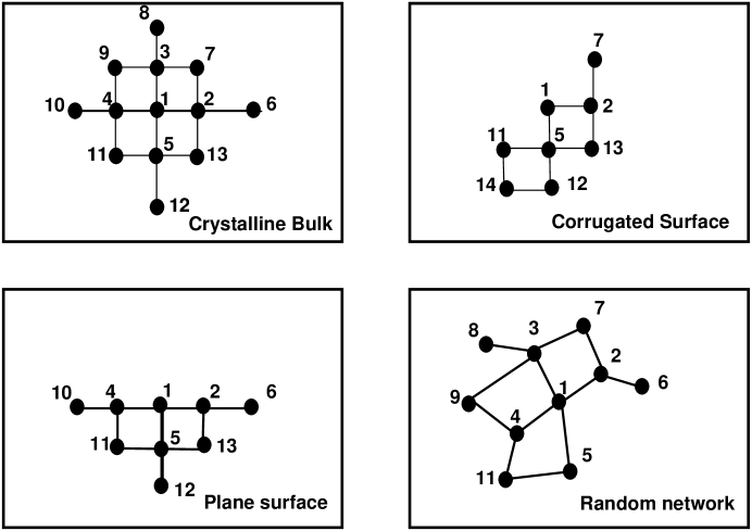
Figure 1: The geometry of (top,left) a bulk square lattice (bottom,left) a square lattice with a plane (100) surface (top,right) a square lattice with a corrugated (110) surface and (bottom,right) a fourfold coordinated planar network

Since the integer numbering increases always clockwise from a site, the directionality is preserved. The neighbour maps, also preserving directionality, for the first three examples are :

$$\hskip-28.45274pt\left(\begin{array}[]{cccc|c}2&\ 3&\ 4&\ 5&\ 4\\ 6&\ 7&\ 1&\ 13&\ 4\\ 7&\ 8&\ 9&\ 1&\ 4\\ 1&\ 9&\ 10&\ 11&\ 4\\ 13&\ 1&\ 11&\ 12&\ 4\\ &&\ \vdots&&\\ \end{array}\right)\enskip;\enskip\left(\begin{array}[]{cccc|c}2&\ -&\ 4&\ 5&\ 3\\ 6&\ -&\ 1&\ 13&\ 3\\ -&\ -&\ -&\ -&\ -\\ 1&\ -&\ 10&\ 11&\ 3\\ 13&\ 1&\ 11&\ 12&\ 4\\ &&\ \vdots&&\\ \end{array}\right)\ ;\ \left(\begin{array}[]{cccc|c}2&\ -&\ -&\ 5&\ 2\\ -&\ 7&\ 1&\ 13&\ 3\\ -&\ -&\ -&\ -&\ -\\ -&\ -&\ -&\ -&\ -\\ 13&\ 1&\ 11&\ 12&\ 4\\ &&\ \vdots&&\\ \end{array}\right)$$

The first four columns give us the neighbours in these four directions and the last column gives us the number of neighbours. For the fourth example of a fourfold coordinated planar random network, the neighbour map is the same for the square lattice, however the S is different.

The action of S on a vector $|n\rangle$ is prompted by the relevant neighbour map. The operations proceed as follows  :

1. One by one choose rows $\underline{n}\/_{i}$ of $|n\rangle$

2. From the neighbour map choose $m=N_{ik}$ (which is the $k$-th neighbour of $i$)

3. Multiply $\underline{\underline{S}}\/_{mi}\underline{n}\/^{T}_{i}$ and add this to the $m$-th row of a new $|n^{\prime}\rangle$

4. Repeat this for all the non-zero rows of $|n\rangle$. Finally $|n^{\prime}\rangle={\mathbf{S}}|n\rangle$.

The the recursive operations described in Eqns. (4) can be encoded into the following modules :

A. Module HOP($|\Phi_{2}\rangle;|\Phi_{1}\rangle$), which describes the action of the Hamiltonian on a ‘vector’.
$\displaystyle\mathrm{The\ input}$ $\displaystyle\mathrm{into}$ $\displaystyle\mathrm{this\ module\ is:}\quad|n\rangle\Rightarrow|\Phi_{2}\rangle$ $\displaystyle{\bf\Delta}^{1/2}|\Phi_{2}\rangle$ $\displaystyle\Rightarrow$ $\displaystyle|\Psi_{1}\rangle\enskip;\enskip{\bf S}|\Psi_{1}\rangle\Rightarrow|\Psi_{2}\rangle\enskip;\enskip{\bf\Delta}^{1/2}|\Psi_{2}\rangle\Rightarrow|\Psi_{1}\rangle$ $\displaystyle({\bf C-E}_{\nu})|\Phi_{2}\rangle$ $\displaystyle\Rightarrow$ $\displaystyle|\Psi_{2}\rangle\enskip;\enskip|\Phi_{1}\rangle=|\Psi_{2}\rangle+|\Psi_{1}\rangle\equiv{\bf h}|n\rangle$ $\displaystyle{\bf o}|\Phi_{1}\rangle$ $\displaystyle\Rightarrow$ $\displaystyle|\Psi_{3}\rangle\equiv{\bf o}{\bf h}|n\rangle$ $\displaystyle{\bf\Delta}^{1/2}|\Psi_{3}\rangle$ $\displaystyle\Rightarrow$ $\displaystyle|\Psi_{1}\rangle\enskip;\enskip{\bf S}|\Psi_{1}\rangle\Rightarrow|\Psi_{2}\rangle\enskip;\enskip{\bf\Delta}^{1/2}|\Psi_{2}\rangle\Rightarrow|\Psi_{1}\rangle$ $\displaystyle({\bf C-E}_{\nu})|\Psi_{3}\rangle$ $\displaystyle\Rightarrow$ $\displaystyle|\Psi_{2}\rangle\enskip;\enskip|\Phi_{1}\rangle=|\Phi_{1}\rangle-|\Psi_{2}\rangle-|\Psi_{1}\rangle\equiv\left[{\bf h}-{\bf hoh}\right]|n\rangle$ $\displaystyle{\bf E}_{\nu}|\Phi_{2}\rangle$ $\displaystyle\Rightarrow$ $\displaystyle|\Psi_{1}\rangle\enskip;\enskip|\Phi_{1}\rangle=|\Phi_{1}\rangle+|\Psi_{1}\rangle\equiv{\bf H}^{(2)}|n\rangle$ $\displaystyle\mathrm{The\ output}$ $\displaystyle\mathrm{from}$ $\displaystyle\mathrm{this\ module\ is}\quad|\Phi_{1}\rangle\Rightarrow{\bf H}^{(2)}|n\rangle$ B. The Module REC( $|\Phi_{2}\rangle,|\Phi_{3}\rangle,\beta_{n}^{2};\alpha_{n},\beta_{n+1}^{2}$) which calculates the coefficients $\alpha_{n},\beta^{2}_{n+1}$ recursively :
$\displaystyle\mathrm{The\ input\ }$ $\displaystyle\mathrm{into\ }$ $\displaystyle\mathrm{this\ module\ is\ :}\quad|\Phi_{2}\rangle\equiv|n\rangle\ ;\ |\Phi_{3}\rangle\equiv|n-1\rangle\ \mbox{and}\ \beta^{2}_{n}$ $\displaystyle\mathrm{Run\ }$ $\displaystyle\Rightarrow$ $\displaystyle\mathrm{HOP}(|\Phi_{2}\rangle;|\Phi_{1}\rangle)\quad\alpha_{n}=\langle\Phi_{1}|\Phi_{1}\rangle/\langle\Phi_{2}|\Phi_{2}\rangle$ $\displaystyle|\Phi_{1}\rangle$ $\displaystyle=$ $\displaystyle|\Phi_{1}\rangle-\alpha_{n}*|\Phi_{2}\rangle-\beta^{2}_{n}*|\Phi_{3}\rangle\quad\beta^{2}_{n}=\langle\Phi_{1}|\Phi_{1}\rangle/\langle\Phi_{2}|\Phi_{2}\rangle$ $\displaystyle|\Phi_{3}\rangle$ $\displaystyle=$ $\displaystyle|\Phi_{2}\rangle\mbox{ and }|\Phi_{2}\rangle=|\Phi_{1}\rangle$ $\displaystyle\mathrm{The\ output}$ $\displaystyle\mathrm{from}$ $\displaystyle\mathrm{this\ module\ is:}\ |\Phi_{2}\rangle\equiv|n+1\rangle;|\Phi_{3}\rangle\equiv|n\rangle\ \mbox{and}\ \alpha_{n},\beta^{2}_{n}$

The two vectors $|\Phi_{1}\rangle$ and $|\Phi_{2}\rangle$ are input/output vectors of the Module HOP, while the three vectors $|\Psi_{1}\rangle,|\Psi_{2}\rangle$ and $|\Psi_{3}\rangle$ are dummies which are needed within the module. The space for these dummies may be dynamically allocated during this procedure and released after the operation is over. The same is true for the vector $|\Phi_{1}\rangle$ in the Module REC.

Eqn. (5) indicates that in the new basis the Hamiltonian representation is tri-diagonal. It follows immediately that The Green function for the system is given by a continued fraction :

$$G_{{\vec{R}}_{i}L,{\vec{R}}_{i}L}(z)=\langle 1|G(z)|1\rangle=\frac{\displaystyle 1}{\displaystyle z-\alpha_{1}-\frac{\displaystyle\beta^{2}_{1}}{\displaystyle z-\alpha_{2}-\frac{\displaystyle\beta^{2}_{2}}{\displaystyle\ddots z-\alpha_{n_{0}}-\beta^{2}_{n_{0}}T(z)}}}$$

(7)

The asymptotic part of the Green function $T(z)$ is called the Terminator. Many terminators are available in literature. The suitable one depends upon the way in which the coefficients $\alpha_{n},\beta^{2}_{n}$ behave as $n\rightarrow\infty$. The most commonly used is the square root terminator which is suitable when $\{\alpha_{n},\beta^{2}_{n}\}\rightarrow\{\alpha,\beta^{2}\}$. Luchini and Nex [14] have suggested a modification when calculations up to a large $n_{0}$ is not possible. If we carry out the terminator approximation after $n_{0}$ steps the first $2n_{0}$ moments of the density of states are exact and it has been shown that the asymptotic moments are also accurately reproduced. Beer and Pettifor [15] have suggested an alternative way of obtaining the terminator. They note that $T(z)=T(z,\{\alpha_{n},\beta_{n}\},n\leq n_{0})$ so that the Beer-Pettifor prescription is a closed algorithm. It wins over the square-root terminator described above when the convergence of the coefficients is either oscillatory or slow. Viswanathan and Muller [16] have suggested several other terminators like the terminator with an exponential tail, suitable when $\beta^{2}_{n}\rightarrow n$ and the terminator with a Gaussian tail, suitable when $\beta^{2}_{n}\rightarrow n^{2}$. We shall have options for several terminating procedures so that the user may choose according to his need. C. The Module GREEN($L_{max},n_{0},E_{min},E_{max}$) which calculates the Green function.
$\displaystyle\mathrm{Loop}$ $\displaystyle(L=1,L_{max})$ $\displaystyle\mathrm{Input}$ $\displaystyle\Rightarrow$ $\displaystyle|\Phi_{2}\rangle=|{\vec{R}}_{i}L\rangle,\ |\Phi_{3}\rangle=|0\rangle\ ;\ \beta^{2}_{0}=1$ $\displaystyle\quad\mathrm{Loop}$ $\displaystyle(n=1,n_{0})$ $\displaystyle\mathrm{Run}$ $\displaystyle\Rightarrow$ $\displaystyle\mathrm{REC}(|\Phi_{2}\rangle;|\Phi_{3}\rangle;\alpha_{n},\beta^{2}_{n})$ $\displaystyle\mathrm{End\ Loop}$ $\displaystyle\mathrm{End\ Loop}$ $\displaystyle\mathrm{Loop}$ $\displaystyle(L=1,L_{max})$ $\displaystyle\mathrm{Loop}$ $\displaystyle(E=E_{min},E_{max})$ $\displaystyle\mathrm{Run}$ $\displaystyle\Rightarrow$ $\displaystyle\mathrm{TERM}(\{\alpha_{n},\beta^{2}_{n}\},n_{0},E,G)$ $\displaystyle\mathrm{Loop}$ $\displaystyle(n=n_{0},1,-1)$ $\displaystyle G$ $\displaystyle=$ $\displaystyle\frac{1}{E-\alpha_{n}-\beta^{2}_{n}*G}$ $\displaystyle\mathrm{End\ Loop}$ $\displaystyle\mathrm{End\ Loop}\enskip\Rightarrow\enskip\mbox{Output}=G_{{\vec{R}}_{i}L,{\vec{R}}_{i}L}(E)$

The partial density of states, projected onto a particular $({\vec{R}}_{i}L)$, is :

$$n_{{\vec{R}}_{i}L}(E)=-\frac{1}{\pi}\ \lim_{\delta\rightarrow 0}\Im m\ G_{{\vec{R}}_{i}L,{\vec{R}}_{i}L}(E+i\delta)$$ (8)

It is clear from this discussion that the recursion procedure is general enough to deal with lattices of any complexity, surfaces and interfaces and disordered networks.

4 The augmented space formalism

Finally we come to the main part of the package : that which deals with disorder. The augmented space formalism [6] allows us to directly compute the configuration average of the Green function by constructing a Hamiltonian in the augmented space of configurations of the random parameters. The formalism is based on ideas prevalent in quantum measurement theory : we associate with each random parameter $n_{i}$ an operator $N_{i}$ whose spectrum $\{n^{\lambda}_{i}\}$ are the measured values of the parameter. The configuration state of $n_{i}$ are the eigenkets $\{|n^{\lambda}_{i}\rangle\}$ of $N_{i}$, which, therefore is an operator in the space ${\cal{C}}_{i}$ spanned by the different configuration states. Given this, the probability density of the parameter is

$$p(n_{i})=-\frac{1}{\pi}\ \Im m\ \langle\emptyset_{i}|\left(\rule{0.0pt}{8.53581pt}(n_{i}+i0)I-N_{i}\right)^{-1}|\emptyset_{i}\rangle$$

where

$$|\emptyset_{i}\rangle=\sum_{\lambda}\ \sqrt{p(\lambda)}|n^{\lambda}_{i}\rangle$$

The augmented space theorem [6] then gives us the configuration average of any function of the random variables :

$$\ll\Phi(\{n_{i}\})\gg=\langle\emptyset|\widetilde{\Phi}(\{N_{i}\})|\emptyset\rangle$$ (9)

Here,

1. $|\emptyset\rangle=\prod^{\otimes}_{i}\ |\emptyset_{i}\rangle$. It is a member of the basis set $|\{C\}\rangle\ =\ \{|n_{1}^{\lambda_{1}},n_{2}^{\lambda_{2}},\ldots\rangle\}$ which spans the configuration space $\Psi$ of the set of random parameters $\{n_{i}\}$.

2. $\widetilde{\Phi}(\{N_{i}\})$ is an operator in the configuration space $\Psi=\prod^{\otimes}{\cal{C}}_{i}$. It is the same operator functional of $\{N_{i}\}$ as $\Phi(\{n_{i}\})$ was a function of $\{n_{i}\}$.

3. The expression is exact. The configuration average is done exactly first, then the approximations may be carried out maintaining various physical constraints. The philosophy is very different from the mean-field approximations like the CPA.

If we apply this to the configuration averaged Green function of a random Hamiltonian $H^{(2)}(\{n_{i}\})$ :

$$\ll G_{{\vec{R}}_{i}L,{\vec{R}}_{i}L}(z,\{n_{i}\})\gg=\langle R_{i}\otimes\emptyset|\left(\rule{0.0pt}{8.53581pt}z\underline{\underline{\widetilde{I}}\/}\/-\underline{\underline{\widetilde{H}}\/}\/^{(2)}(\{\widetilde{N}_{i}\}\right)^{-1}|R_{i}\otimes\emptyset\rangle$$

(10)

Let us take as an example the case of a disordered binary alloy : the Hamiltonian has the same form as Eqn. (2) but :

$$\underline{\underline{\widehat{C}}\/}\/_{i} = \underline{\underline{\widehat{C}}\/}\/_{A}\ n_{i}+\underline{\underline{\widehat{C}}\/}\/_{B}\ (1-n_{i})\quad\mbox{where}\quad\underline{\underline{\widehat{C}}\/}\/_{i}=\underline{\underline{C}\/}\/_{i}-\underline{\underline{E}\/}\/_{\nu}\quad\mbox{and}\quad$$

$$\underline{\underline{\Delta}\/}\/^{1/2}_{i} = \underline{\underline{\Delta}\/}\/^{1/2}_{A}\ n_{i}+\underline{\underline{\Delta}\/}\/^{1/2}_{B}\ (1-n_{i})\quad\mbox{and}\quad\underline{\underline{o}}\/_{i}=\underline{\underline{o}\/}\/_{A}\ n_{i}+\underline{\underline{o}\/}\/_{B}\ (1-n_{i})$$

The random “occupation” variables $n_{i}$ take the values 0 and 1 with probabilities proportional of the concentrations x and y of the constituents A and B. $N_{i}$ has a $2\times 2$ representation : $\left(\begin{array}[]{cc}x&\sqrt{xy}\\ \sqrt{xy}&y\end{array}\right)$ . If we denote the basis of the above representation by $|\uparrow_{i}\rangle,|\downarrow_{i}\rangle$, then

$$\widetilde{N}_{i}=x{\cal I}+(y-x){\cal P}_{\downarrow_{i}}+\sqrt{xy}{\cal T}_{\uparrow_{i}\downarrow_{i}}$$

and each of the potential parameters become operators in the configuration space, for example :

$$\widetilde{\mathbf{C}} = \sum_{i}\left\{\rule{0.0pt}{8.53581pt}\ll\underline{\underline{\hat{C}}}\/_{i}\gg\ {\cal I}+\ B(\underline{\underline{\hat{C}}}\/_{i})\ {\cal P}_{\downarrow_{i}}+\ F(\underline{\underline{\hat{C}}}\/_{i})\ {\cal T}_{\uparrow_{i}\downarrow_{i}}\right\}\otimes{\cal P}_{i}$$

$${\widetilde{\mathbf{\Delta}}}^{1/2} = \sum_{i}\left\{\rule{0.0pt}{8.53581pt}\ll\underline{\underline{{\Delta}}}\/^{1/2}_{i}\gg\ {\cal I}+\ B(\underline{\underline{{\Delta}}}\/^{1/2}_{i})\ {\cal P}_{\downarrow_{i}}+\ F(\underline{\underline{{\Delta}}}\/^{1/2}_{i})\ {\cal T}_{\uparrow_{i}\downarrow_{i}}\right)\otimes{\cal P}_{i}$$

$${\widetilde{\mathbf{E}}}_{\nu} = \sum_{i}\left\{\rule{0.0pt}{8.53581pt}\ll\underline{\underline{{E}}}\/_{\nu}\gg\ {\cal I}+\ B(\underline{\underline{{E}}}\/_{\nu})\ {\cal P}_{\downarrow_{i}}+\ F(\underline{\underline{E}}\/_{\nu})\ {\cal T}_{\uparrow_{i}\downarrow_{i}}\right\}\otimes{\cal P}_{i}$$

$${\widetilde{\mathbf{o}}} = \sum_{i}\left\{\rule{0.0pt}{8.53581pt}\ll\underline{\underline{{o}}}\/_{i}\gg\ {\cal I}+\ B(\underline{\underline{{o}}}\/_{i})\ {\cal P}_{\downarrow_{i}}+\ F(\underline{\underline{\hat{o}}}\/_{i})\ {\cal T}_{\uparrow_{i}\downarrow_{i}}\right\}\otimes{\cal P}_{i}$$ (11)

where $B(C)=(y-x)(C_{A}-C_{B})$ and $F(C)=\sqrt{xy}(C_{A}-C_{B})$. Also, since the structure matrix is not random :

$${\widetilde{\mathbf{S}}}=\sum_{ij}\underline{\underline{S}}\/_{{\vec{R}}_{i}{\vec{R}}_{j}}\ {\cal I}\otimes{\cal T}_{ij}$$ (12)

$${\widetilde{\mathbf{H}}}^{(2)} = {\widetilde{\mathbf{E}}}_{\nu}+{\widetilde{\mathbf{h}}}-{\widetilde{\mathbf{h}}}\ {\widetilde{\mathbf{o}}}\ {\widetilde{\mathbf{h}}}\quad\mbox{where}\quad{\widetilde{\mathbf{h}}}={\widetilde{\mathbf{C}}}+{\widetilde{\mathbf{\Delta}}}^{1/2}\otimes{\widetilde{\mathbf{S}}}\otimes{\widetilde{\mathbf{\Delta}}}^{1/2}$$ (13)

If we now compare Eqns. (10) and (13) with Eqns. (6)-(7) it becomes clear that once we have defined the Hamiltonian in the space of configurations, the recursion method may be directly used to obtain the configuration averaged Green function. The approximation involved will then only be the “termination” approximation. Heine’s “Black-body theorem” [17] indicates that most electronic structure energetics is dominated by the immediate environment of a site. This is a major justification of the termination approximation. Unlike the CPA which gives only the first eight moments of the density of states exactly and the asymptotic moments accurately, the augmented space recursion gives $2n_{0}$ moments exactly (where the termination is done after $n_{0}$ steps) and the asymptotic moments also accurately. In most of our calculations we can take $n_{0}$ about 8-9 steps.

5 The TB-LMTO-ASR Algorithm

The full package is divided into several modules. The first is the Preparation Module. This module has two branches, one each for each constituent of the alloy. Each branch runs parallely in two different slave processors. The structure matrix is prepared in the master processor. This Module prepares the following :

1. It prepares the two control files for the different alloy constituents. This part is interactive with the user.

2. It carries out the simple Hartree calculation and prepares the atomic radii of the constituents and the initial charge density.

3. It calculates the overlap between atomic spheres and inputs empty spheres maintaining the symmetries.

4. It calculates the structure matrix from the inputs of the control files.

Figure 2: (Color Online) The TB-LMTO-Augmented Space Recursion package flowchart

The Preparation Module is followed by the main ASR-module. This module is called by the routine lmasr. This main module is divided into five smaller modules :

• Module A : This module reads the data generated by the Preparation Module. It checks the inputs for consistency. The routines in this module are again those in the Stuttgart LMTO47, but modified to read the inputs for both the two constituents of the alloy.

• Module B: At the start of the DFT self-consistency loop, this module takes the overlap of a simple Hartree atomic density calculation in the Preparation module and generates the Hartree and exchange-correlation potentials, spheridizes them and inputs them to the Atomic Module that follows. In later steps of the self-consistency loop, this Module first mixes the charge densities of the earlier steps and prepares the Hartree and exchange-correlation potentials,spheridizes them for input into the Atomic Module.

  - At this point there is a choice of using either the standard DFT exchange-correlation potentials or, alternatively, there is a branch module Harbola-Sahni which sets up the Harbola-Sahni potential for the study of excited states [19].

• Module C: This is the Atomic Module. It takes the spheridized Kohn-Sham potential generated in Module B and solves the radial Kohn-Sham equation numerically. The Kohn-Sham orbitals and energies then lead to the potential parameters for each constituent. Those for the two constituents are calculated on different processors. The parameters are first calculated in the orthogonal representation. A new routine gtoa, not present in the Stuttgart LMTO47 package, then transforms them to the most screened tight-binding representation.

• Module D : This is the main ASR Module. The routines herein have been fully developed by us and form the main backbone of the package. The input are the tight-binding Hamiltonian parameters from the Atomic Module. First they are combined with the alloy composition to prepare the augmented space Hamiltonian. The nearest neighbour map in augmented space is then generated. Next, the recursion is carried out for each $L$ value, terminators generated and the $L$ projected density of states are calculated. Each different recursion for each $L$ value is carried out on a different processor, thus vastly accelerating the calculations.

  We then proceed to calculate the total density of states and the Fermi energy. Again, branching out into different processors, we calculate the $L$-dependent moments and magnetic moments. Of all the Modules, this is the one amenable to maximum parallelization.

  - At this point we have the possibility of introducing short ranged order.The ASR for short-ranged order has been described in some detail earlier [20]. The branching for this choice occurs just before we set up the augmented space Hamiltonian. The extra input is the Warren-Cowley short ranged order parameter.

  - Also at this point we have the option to introducing disorder in the structure matrix because of size mismatch between the two constituents of the alloy. The branching now takes place earlier in the Preparation Module where we generate not one, but three different structure matrices : $\underline{\underline{S}}\/^{AA}_{ij},\underline{\underline{S}}\/^{BB}_{ij}$ and $\underline{\underline{S}}\/^{AB}_{ij}$. In the ‘end point’ approximation [21] the Eqn. (12) is now replaced by :

  $${\widetilde{\mathbf{S}}}=\sum_{ij}\left\{\rule{0.0pt}{8.53581pt}\ll\underline{\underline{S}}\/_{ij}\gg{\cal I}+\underline{\underline{S}}\/^{(1)}_{ij}\left({\cal N}_{i}+{\cal N}_{j}\right)+\underline{\underline{S}}\/^{(2)}_{ij}{\cal N}_{i}\otimes{\cal N}_{j}\right\}\otimes{\cal T}_{ij}$$ (14)

  where ${\cal N}_{i}=(y-x){\cal P}_{\downarrow_{i}}+\sqrt{xy}{\cal T}_{\uparrow_{i}\downarrow_{i}}$, $\underline{\underline{S}}\/^{(1)}=\underline{\underline{S}}\/^{AB}_{ij}-\underline{\underline{S}}\/^{BB}_{ij}$ and $\underline{\underline{S}}\/^{(2)}=\underline{\underline{S}}\/^{AA}_{ij}+\underline{\underline{S}}\/^{BB}_{ij}-2\underline{\underline{S}}\/^{AB}_{ij}$. This modification will be available in this module.

  It is in these last two options that the ASR really scores over the CPA, which cannot really deal with either short-ranged order or off-diagonal disorder as both involve more than one site. The competing methodology is the special quasi-random structures (SQS) [22]. However, if we are dealing with materials with many atoms per unit cell and non-stoichiometric compositions, the SQS required will be rather large and will involve use of huge unit cells. Here the TB-LMTO-ASR with the use of much smaller unit cells will score. We have shown earlier [23] that both these two methods give virtually the same results for the density of states.

• Module E : In this module the $L$-dependent moments are used to obtain the charge density. We also calculate the total energy, including the Madelung term. For the disordered alloy, the Madelung term is obtained from the procedure suggested by Skriver and Ruban [24]. Finally the old and new moments are mixed, the mixed charge density thus obtained is input back in Module B. This is iterated till convergence in both energy and charge density is achieved.

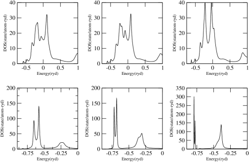
Figure 3: (Top) DOS for Cr_xFe_1-x for different compositions : (left) Cr₇Fe₃; (middle) Cr₅Fe₅; (right) Cr₃Fe₇; (Bottom) DOS for Cu_xZn_1-x for different compositions : (left) Cu₂₄Zn₇₆; (middle) Cu₅₀Zn₅₀; (right) Cu₇₅Zn₂₅. Energy(Ryd) is plotted along $x$-axis; $y$-axis is DOS (states/Ryd)

For the DFT part, our code depends heavily on Stuttgart-LMTO routines developed by Anderson and co-workers [25] Two independent DFT codes run parallely to produce the potential parameters of the two constituent atoms of the binary alloy. These potential parameters are used at the input point of our ASR routines in Module D.

Our present DFT modules deal only with collinear magnetism. For spin dependent calculations the Hamiltonian is separable in spin space. Thus the spin is merged with the label $L$ which is now $\{\ell,m,\sigma\}$ and we have just to carry out twice the number of recursions : for $\sigma=\uparrow$ and $\downarrow$. In case we wish to introduce spin-orbit coupling and possibility of non-collinear magnetism, we have to replace the DFT module with one dealing with density matrices, rather than densities [26] and the ASR module with one applying generalized or vector recursion [12]-[13] which was designed to deal with Hamiltonians whose representation in spin-space or ‘spinor’ bases is not diagonal :

$$\ll\underline{\underline{n}}\/|\underline{\underline{\widetilde{H}}}\/|\underline{\underline{m}}\/\gg=\left(\begin{array}[]{cc}\underline{\underline{H}}\/^{\uparrow\uparrow}_{nm}&\underline{\underline{H}}\/^{\uparrow\downarrow}_{nm}\\ \underline{\underline{H}}\/^{\downarrow\uparrow}_{nm}&\underline{\underline{H}}\/^{\downarrow\downarrow}_{nm}\end{array}\right)\enskip\mbox{where }\enskip|\underline{\underline{n}}\/\gg=\left(\begin{array}[]{c}|n\!\!\uparrow\rangle\\ |n\!\!\downarrow\rangle\end{array}\right)$$

This new module is under preparation [27] and will be incorporated once the basic checks are carried out. Here we mention this in order to bring out the different possibilities and versatility of the package.

6 Applications and performance analysis

We have described the contents and commented upon the efficiency and versatility of the TB-LMTO-ASR package. We shall conclude by describing two different applications : namely, the alloys $\textrm{Cu}_{x}\textrm{Zn}_{1-x}$ where both the constituents are non-magnetic in the bulk and the $d$-band centres of Cu and Zn are well separated; and Fe_xCr_1-x where both constituents are magnetic and their $d$-bands overlap.

For a single self-consistency loop
	Old TB-LMTO-ASR	New TB-LMTO-ASR
Wall time	699 sec	225 sec
Efficiency$\left(\frac{\rm cputime}{\rm walltime}\right)$	0.714	0.97

The alloys have been studied earlier by us using the old version of the TB-LMTO-ASR [4],[28]-[29] and TB-LMTO-CCPA [31], both introduced by us, and the KKR-ICPA [32] which is also based on the augmented space formalism, as well as through the KKR-CPA [34], PAW-SQS[22] and KKR-NL-CPA [35]-[36]. They are therefore ideal system for benchmarking the new TB-LMTO-ASR package. Comparison of the densities of states shown in Fig. 3 with the results shown in the above references will convince us that for Fe_xCr_1-x there is hardly anything to choose between the various techniques and the packages based on them. However, for the split band alloy Cu_xZn_1-x the TB-LMTO-ASR, TB-LMTO-CCPA and KKR-NL-CPA scores over the CPA versions, as expected from earlier analysis.

One of our our main point of interest is the relative runtime and efficiency of this new version of the TB-LMTO-ASR, as compared to the several earlier versions proposed by us. To benchmark these characteristics we take a specific calculation on Fe_xCr_1-x. Each calculation is done on a 73109 site augmented space map, with N recursion steps with $L=s,p_{x},e_{g}$ and $t_{2g})$, and $\sigma=1,2$, followed by a Beer-Pettifor termination scheme . The old and new versions of the TB-LMTO-ASR are compared in the Table 6. Here Wall time is the same as run time and Efficiency is the ratio between the Wall time and CPU time. Gnu profiles (gprof) for the new TB-LMTO-ASR output and the old serial version are given in the Table (1).

%	cumulative	self		self	total
time	seconds	seconds	calls	s/call	s/call	name
49.91 (61.47)	100.73 (397.33)	100.73 (397.33)	81 (128)	1.24 (3.10)	2.26 (5.01)	hop
40.78 (37.67)	183.04 (640.87)	82.31 (243.54)	1.6$(3.9)\times 10^{9}$	0.00 (0.00)	0.00 (0.00)	matp
0.76 (0.79)	196.82 (646.41)	1.53 (5.11)	7(16)	0.22 (0.00)	0.22 (0.32)	spectral
0.00 (0.00)	201.84 (646.40)	0.00 (0.01)	1.8 (3.5) $\times 10^{5}$	0.00 (0.00)	0.00(0.00)	splint
0.00 (0.00)	201.84 (646.44)	0.00 (0.00)	206 (384)	0.00 (0.00)	0.00 (0.00)	spline
0.00 (0.00)	201.84 (646.44)	0.00 (0.00)	56 (56)	0.00 (0.00)	0.00 (0.00)	matmult
0.00 (0.00)	201.84 (646.44)	0.00 (0.00)	36 (36)	0.00 (0.00)	0.00 (0.00)	mom
0.00(*)	201.84 (*)	0.00 (*)	28 (*)	0.00 (*)	6.59 (*)	doparallel
0.00 (0.00)	201.84 (646.44)	0.00 (0.00)	7 (16)	0.00 (0.00)	0.00 (0.00)	fit
0.00 (0.00)	201.84 (646.44)	0.00 (0.00)	4 (7)	0.00 (0.00)	0.00 (0.00)	tdos
0.00 (0.00)	201.84 (646.44)	0.00 (0.00)	1 (1)	0.00 (0.00)	0.00 (0.00)	band
0.00 (0.00)	201.84 (646.44)	0.00 (0.00)	1 (1)	0.00 (0.00)	0.00 (0.00)	fermi
0.00 (0.00)	201.84 (646.44)	0.00 (0.00)	1 (1)	0.00 (0.00)	0.00 (0.00)	pardos

Table 1: gprof data for the optimized and parallelized ASR code and (in brakets) the old serial code. The discontinuity between the cumulative time of spectral and splint is due to the machine routine which are not included here.

7 Conclusion

We have presented here a computational package that combines three different techniques to allow us to study the electronic properties of disordered systems. The package can deal with bulk disordered alloys as well as surfaces and interfaces, both smooth, stepped and rough and also structurally distorted lattices. The package can be generalized at many stages which have been clearly commented upon and the generalizations are being carried out step by step.

References

- [1] R. Haydock, V. Heine, and M. Kelly, J. Phys. C 5 (1972) 2845
- [2] R. Haydock, V. Heine, and M. Kelly., J. Phys. C 8 (1975) 2591
- [3] A. Mookerjee in Electronic structure of alloys, surfaces and clusters (Taylor-Francis,UK) ed. D.D. Sarma and A. Mookerjee (2003).
- [4] A. Chakrabarti and A. Mookerjee,E. Phys. J. B44 (2005) 21
- [5] Andersen O K, Kasowski R V, Phys. Rev. B 4 (1971) 1064
- [6] A. Mookerjee, J. Phys. C 6 (1973) 1340
- [7] R.V. Kasowski, O.K. Andersen O K, Solid State Commun. 11 (1972) 1064
- [8] O.K. Andersen, R.G.Woolley, Mol.Phys. 28 (1973) 905
- [9] O.K. Andersen, Phys. Rev. B 12 (1975) 3060
- [10] S. Ghosh, N. Das and A. Mookerjee, Int J. Mod. Phys. B13 (1999) 723
- [11] J.M. Wills, O. Eriksson and M. Aloouani, in Structure and physical properties of solids ed. H. Dreyseé (Berlin, Springer-Verlag) (2000) 148
- [12] T. J. Godin, R. Haydock, Phys. Rev. 38, (1988) 5237
- [13] T. J. Godin, R. Haydock, Comp. Phys. Comm. 64 (1991) 123
- [14] N.U. Luchini and C.M.M. Nex , J. Phys. C (Solid State) 20 (1987) 3125
- [15] N. Beer and D. G. Pettifor, in The Electronic Structure of Complex Systems, ed. P. Phariseau and W. M. Temmerman, (Plenum, New York, 1982), 113 769
- [16] V.S. Viswanath and G. Müller , in “The user friendly recursion method”, (Troisieme Cycle de la Physique, en Suisse Romande) (1993)
- [17] V. Heine, in ’Solid State Theory’ vol 35 (Academic Press, New York) (1980)
- [18] O. K. Andersen, Phys. Rev. B 12 (1975) 3060
- [19] M. Rahaman, S. Ganguly, P. Samal, T. Saha-Dasgupta, A. Mookerjee and M.K. Harbola, Physica B : Condens Matter 404 (2009) 1137
- [20] A. Mookerjee A. and R. Prasad R., Phys. Rev. B 48 (1993) 17724
- [21] T. Saha and A. Mookerjee, J. Phys.: Condens. Matter 8 (1996) 2915
- [22] A. Zunger, S.H.- Wei, L.G. Ferreira and J. Bernard, Phys. Rev. Lett 65 (1990) 353
- [23] K. Tarafder, S. Ghosh. B. Sanyal, O. Eriksson, A. Mookerjee and A.Chakrabarti, J. Phys.: Condens. Matter 20 (2008) 445201
- [24] A.V. Ruban and H.L. Skriver, Phys. Rev. 66 (2003) 024201
- [25] O.K. Andersen and O. Jepsen, Phys. Rev. Lett53 (1984) 2571
- [26] R. Lizárraga, S. Ronnenteg,R. Berger, A. Bergman, P. Mohn, O. Erikkson and L. Nordström, Phys. Rev. B 70 (2004) 024407
- [27] S. Ganguli, A. Bergman and A. Mookerjee, (under preparation) (2009)
- [28] T. Saha, I. Dasgupta and A. Mookerjee, Phys. Rev. B 50 (1994) 13267
- [29] T. Saha, I. Dasgupta and A. Mookerjee, J. Phys.: Condens. Matter 8 (1996) 1979
- [30] A. Chakrabarti and A. Mookerjee, E. Phys. J. B 44 (2005) 21
- [31] M. Rahaman and A. Mookerjee, Phys. Rev. B 79 (2009) 054201
- [32] S. Ghosh, P.L. Leath and M.H. Cohen Phys. Rev. B66, (2003) 214206
- [33] A. Chakrabarti and A. Mookerjee, E. Phys. J. B 44 (2005) 21
- [34] P.E.A. Turchi, L. Reinhard and G.M. Stocks, Phys. Rev. B 50, (1994) 15542
- [35] M. Jarrell and H.R. Krishnamurthy, Phys. Rev. B 63 (2001) 125102
- [36] D.A. Rowlands, J.B. Staunton, B.L. Gyorffy, E. Bruno and B. Ginatempo, Phys. Rev. B 72 (2005) 045101