Cosmic Ray Spectra in Nambu-Goldstone Dark Matter Models

Abstract

We discuss the cosmic ray spectra in annihilating/decaying Nambu-Goldstone dark matter models. The recent observed positron/electron excesses at PAMELA and Fermi experiments are well fitted by the dark matter with a mass of 3 TeV for the annihilating model, while with a mass of 6 TeV for the decaying model. We also show that the Nambu-Goldstone dark matter models predict a distinctive gamma-ray spectrum in a certain parameter space.

I Introduction

Recent observations of the PAMELA Adriani:2008zr , ATIC Chang:2008zz , PPB-BETS Torii:2008xu , and Fermi Abdo:2009zk experiments strongly suggest the existence of a new source of positron/electron fluxes. The most interesting candidate of the new source is the dark matter with a mass in the TeV range annihilating or decaying into the visible particles which result in the positrons/electrons Bergstrom:2009ib . Especially, the Fermi experiment has released data on the electron/positron spectrum from 20 GeV up to 1 TeV Abdo:2009zk , where the spectrum falls as $E^{-3.0}$. As reported in Refs. Murayama:2009 ; Bergstrom:2009fa ; Meade:2009iu the data can be well fitted by the dark matter which mainly annihilates/decays into a pair of light scalars each of which subsequently decays into a pair of electrons or muons.

From the theoretical point of view, it is always motivated to relate the identity of the dark matter with the new physics which is anticipated from other motivations Murayama:2007ek . Among them, one of the most motivated new physics is the supersymmetric standard model (SSM) which is expected as a solution to the hierarchy problem. In the SSM, the stable lightest supersymmetric particle (LSP) is a candidate of the dark matter. The LSP interpretation with a mass in the TeV range Shirai:2009fq ; Chen:2009mj , however, implies that the masses of the other supersymmetric particles are much heavier than a TeV, which diminishes the significance of the SSM as a successful solution to the hierarchy problem. Besides, such a heavy LSP interpretation can be falsified rather easily, once the supersymmetric particles are discovered in hundreds GeV range at the coming LHC experiments.

The attempt to relate the dark matter to the supersymmetric models, however, should not be necessarily confined to the LSP dark matter scenarios. In fact, the SSM always requires other new physics, the supersymmetry breaking sector which may include a stable particle as a candidate of the dark matter. The idea of the Nambu-Goldstone dark matter developed in Ref. Ibe:2009dx is one of the realization of the dark matter in a supersymmetry breaking sector. There, the dark matter is interpreted as a pseudo-Nambu-Goldstone boson in a supersymmetry breaking sector so that the mass of the dark matter is in the TeV range out of the dynamics of supersymmetry breaking at tens to hundreds TeV range.

In an explicit example of the Nambu-Goldstone dark matter scenario given in Ref. Ibe:2009dx , we considered the model where the dark matter annihilates into a pair of the light pseudo scalars, the R-axions, via a narrow resonance, the flaton, which leads to the right amount of the dark matter. Furthermore, for the R-axion mainly decaying into a pair of electrons or muons, the final state of the dark matter is the four electrons or muons, which are favored to explain the positron/electron spectrum observed by Fermi experiment.

The most prominent difference of the Nambu-Goldstone dark matter model from the other dark matter models which explain the observed positron/electron excesses is that the Nambu-Goldstone dark matter model is strongly interrelated to the physics of the SSM. That is, in the Nambu-Goldstone dark matter scenario, it is difficult for the supersymmetry breaking to be much higher than tens to hundreds TeV. This restriction suggests that the supersymmetry breaking effects should be mediated to the SSM sector at the low energy scale, i.e., the model requires the gauge mediation mechanism Giudice:1998bp . Thus, the dark matter interactions with the SSM particles are determined along with the gauge mediation effects. With the interrelation to the SSM physics, the Nambu-Goldstone dark matter model has a distinctive prediction on such as a gamma-ray spectrum and an antiproton flux in cosmic ray.

In this paper, we discuss the cosmic ray spectra in the Nambu-Goldstone dark matter scenario based on the explicit model in Ref. Ibe:2009dx . As we will show, the Nambu-Goldstone dark matter model fits to the recently observed positron/electron excesses in both the annihilating and the decaying dark matter scenarios. Furthermore, we show that the model gives a distinctive prediction on a gamma-ray spectrum for a certain parameter space, which comes from the finite annihilation/decay rates of the dark matter into a pair of gluinos.

The organization of the paper is as follows. In section II, we summarize the explicit example of the NDGM model in Ref. Ibe:2009dx . There, we also derive conditions so that the dark matter density is consistent with the observed dark matter density. In section III, we show how well the model fits the observed fluxes in both the annihilating/decaying dark matter scenarios. We also demonstrate how the modes into the SSM particles affect the gamma-ray spectrum.

II Nambu–Goldstone Dark Matter

In this section, we review a model of the Nambu–Goldstone dark matter model Ibe:2009dx which is based on a vector-like SUSY breaking model in Ref. Izawa:1996pk . In the model, the dark matters are interpreted as pseudo Nambu-Goldstone bosons which result from spontaneous breaking of the approximate global symmetry in the vector-like SUSY breaking model.

II.1 Nambu-Goldstone Dark Matter, Flaton, and R-axion

The key ingredients of the model are the light flaton which corresponds to the so-called pseudo moduli of the SUSY breaking model, and the R-axion which is a pseudo Nambu-Goldstone boson resulting from spontaneous R-symmetry breaking. In the followings, we overview the relevant properties of those particles.

II.1.1 SUSY breaking sector

The vector-like SUSY breaking model is based on an $SU(2)$ gauge theory with four fundamental representation fields $Q_{i}(i=1,\cdots,4)$ and six singlet fields $S_{ij}=-S_{ji}$ ($i,j=1,\cdots,4$). In this model, the SUSY is dynamically broken when the $Q$’s and $S$’s couple in the superpotential,

$$W=\lambda_{ij}S_{ij}Q_{i}Q_{j},\,(i<j),$$ (1)

where $\lambda_{ij}$ denote coupling constants. The maximal global symmetry this model may have is $SU(4)\simeq SO(6)$ symmetry which requires $\lambda_{ij}=\lambda$. The SUSY is broken as a result of the tension between the $F$-term conditions of $S$’s and $Q$’s. That is, the $F$-term conditions of $S_{ij}$, $\partial W/\partial S_{ij}=\lambda_{ij}Q_{i}Q_{j}=0$, contradict with the quantum modified constraint ${\rm Pf}(M_{ij})=\Lambda_{\rm dyn}^{2}$ where $M_{ij}$ denote composite gauge singlets made from $Q_{i}Q_{j}$.

Below the dynamical scale $\Lambda_{\rm dyn}$, the model is described by the light degrees of freedom, $M_{A}$ and $S_{A}$, ($A=1-6$), with a quantum modified constraint,

$$\sum_{A=1-6}M_{A}^{2}=\Lambda_{\rm dyn}^{2}.$$ (2)

Here, we have assumed that the effective composite operators $M_{A}$ are canonically normalized. Notice that the above quantum modified constraint breaks the global $SU(4)\simeq SO(6)$ symmetry into $SP(2)\simeq SO(5)$ symmetry. Thus, when the model possesses the $SO(6)$ symmetry approximately, the Nambu-Goldstone bosons appear as the result of the quantum modified constraint. Furthermore, the Nambu-Goldstone bosons have a long lifetime when an appropriate subgroup of $SO(5)$ is almost exact. (We will discuss more on the stability and the global symmetry in the next section.) In this way, we realize a model with the Nambu-Goldstone dark matter with mass in the TeV range out of physics of tens to hundreds TeV range.

To make the discussion concrete, for a while, let us assume that the SUSY breaking sector possesses an $SO(5)\subset SO(6)$ global symmetry and rearrange the tree-level interaction Eq. (1) so that the $SO(5)$ symmetry is manifest;

$$W = \lambda\,S_{0}(QQ)_{0}+\lambda^{\prime}\sum_{a=1-5}S_{a}(QQ)_{a}\ ,$$ (3)

$$= \lambda\,\Lambda_{\rm dyn}S_{0}M_{0}+\lambda^{\prime}\sum_{a=1-5}\Lambda_{\rm dyn}S_{a}M_{a}\ .$$ (4)

In the second line, we rewrite the superpotential by using the low energy field $M_{A}$. We further assume $\lambda<\lambda^{\prime}$ and assume that the model possesses the $SO(6)$ symmetry in the limit of $\lambda\to\lambda^{\prime}$. Under these assumption, the Nambu-Goldstone bosons are charged under the $SO(5)$ symmetry and are stable.

For later convenience, let us solve the quantum modified constraint explicitly by,

$$M_{0}=\sqrt{\Lambda_{\rm dyn}^{2}-\sum_{a=1-5}M_{a}^{2}}\ ,$$ (5)

and plug it into the effective superpotential in Eq. (3);

$$W_{\rm eff} \simeq \lambda\,\Lambda_{\rm dyn}^{2}S_{0}-\sum_{a=1-5}\frac{\lambda}{2}\,S_{0}M_{a}^{2}+\sum_{a=1-5}\lambda^{\prime}\,\Lambda_{\rm dyn}S_{a}M_{a}+O(M_{a}^{4})\ .$$ (6)

From this expression, we see that the SUSY breaking vacuum is given by,

$$F_{S_{0}}=\lambda\Lambda_{\rm dyn}^{2}\ ,\quad S_{a}=0\ ,\quad M_{a}=0\ .$$ (7)

II.1.2 Mass spectrum of $S_{0}$ multiplet

Around the vacuum in Eq. (7), the tree-level potential in the $S_{0}$ direction is flat, and the masses of the $S_{0}$ multiplets can be significantly lighter than the dynamical scale. As discussed in Ref. Ibe:2009dx , this is a quite favorable feature to account for the observed dark matter density. The annihilation cross section of the Nambu-Goldstone dark matter with a mass in the TeV range is generically too small to explain the observed dark matter density (see Ref. Ibe:2009dx for general discussion). In this model, however, the annihilation cross section is enhanced by a narrow resonance which is served by the flaton, a radial component of $S_{0}$. It should be noted that, for that purpose, the R-symmetry must be broken so that the dark matters with R-charge zero annihilate through the flaton resonance with R-charge two.

In Ref. Ibe:2009dx , we considered the model with spontaneous R-symmetry breaking. The spontaneous R-symmetry breaking is caused by effects of higher dimensional operators of $S_{0}$ in the Kähler potential,

$$K = |S_{0}|^{2}+\frac{|S_{0}|^{4}}{4\Lambda_{4}^{2}}-\frac{|S_{0}|^{6}}{9\Lambda_{6}^{4}}+\cdots,$$ (8)

where $\Lambda$’s denote the dimensionful parameters and the ellipsis denotes the higher dimensional terms of $S_{0}$. The above Kähler potential provides an effective description of a quite general class of the models with spontaneous breaking of the R-symmetry breaking. Especially, when the above Kähler potential results from radiative corrections from physics at the scale $\Lambda_{\rm dyn}$, the dimensionful parameters are expected to be,

$$\frac{1}{\Lambda_{4}^{2}}=\frac{c_{4}^{2}}{16\pi^{2}}\frac{1}{\Lambda_{\rm dyn}^{2}},\quad\frac{1}{\Lambda_{6}^{4}}=\frac{c_{6}^{2}}{16\pi^{2}}\frac{1}{\Lambda_{\rm dyn}^{4}},$$ (9)

where dimensionless coefficients $c_{4,6}$ are of the order of unity (see Ref. Ibe:2009dx for an explicit model with R-symmetry breaking). From this Kähler potential, the R-symmetry is spontaneously broken by the vacuum expectation value of the scalar component of $S_{0}$;

$$\left\langle{S_{0}}\right\rangle = \frac{1}{\sqrt{2}}\frac{\Lambda_{6}^{2}}{\Lambda_{4}}=\frac{1}{\sqrt{2}}\frac{c_{4}}{c_{6}}\Lambda_{\rm dyn}=\frac{1}{\sqrt{2}}f_{R},$$ (10)

where we have introduced the R-symmetry breaking scale $f_{R}=O(\Lambda_{\rm dyn})$.

Now let us consider the masses of the scalar components of $S_{0}$. At this vacuum, the scalar component of $S_{0}$ is decomposed into the flaton $s$ and the R-axion $a$ by,

$$S_{0}=\frac{1}{\sqrt{2}}(f_{R}+s)e^{ia/f_{R}}.$$ (11)

Then, the mass of the flaton is given by,

$$m_{s}=4\sqrt{2}\,\frac{\lambda\Lambda_{\rm dyn}^{2}\Lambda_{4}^{3}}{(4\Lambda_{4}^{4}+\Lambda_{6}^{4})}\simeq\sqrt{2}\frac{\lambda\Lambda_{\rm dyn}^{2}}{\Lambda_{4}}\simeq\sqrt{2}\frac{c_{4}}{4\pi}\lambda\Lambda_{\rm dyn},$$ (12)

where we have used $F_{S_{0}}=\lambda\Lambda_{\rm dyn}^{2}$ and assumed Eq. (9) with $c_{4}=c_{6}=O(1)$. Therefore, the flaton can be in the TeV range for $\lambda\sim 1$ and $c_{4}\sim 1$, which is a crucial property for the flaton to make the narrow resonance appropriate for the dark matter annihilation.

The R-axion mass, on the other hand, can be much more suppressed, since it is a pseudo-Goldstone boson of the spontaneous R-symmetry breaking. For example, when explicit breaking of the R-symmetry mainly comes from the constant term in the superpotential, the R-axion acquires a small mass Bagger:1994hh ,

$$m_{\mathrm{axion}}^{2}\sim\frac{m_{3/2}F_{S_{0}}}{f_{R}}.$$ (13)

This mass is in a MeV range for $f_{R}\simeq\sqrt{F_{S_{0}}}\simeq 30$ TeV and $m_{3/2}\simeq 1$ eV, for example.

The most interesting feature of the R-axion in the above mass range is that it mainly decays into an electron pair Goh:2008xz . Therefore, the dark matter which annihilates (or decays) into a pair of the R-axions ends up with the final states with four electrons. In section III, we see that the four electron final states of the dark matter annihilation or decay are favorable to explain the positron/electron spectra. Notice that there is a lower limit on the decay constant $f_{R}$ of the axion-like particles which mainly decay into pairs of electrons from the beam-dump experiments Bergsma:1985qz ;

$$f_{R}\gtrsim 10\,{\rm TeV}\times\left(\frac{m_{a}}{1\,{\rm MeV}}\right)^{1/2}\quad\mbox{for }1\,{\rm MeV}\lesssim m_{a}\lesssim 100\,{\rm MeV}.$$ (14)

On the other hand, as we will see in section II.3, the right amount of dark matter requires $f_{R}\simeq 30$ TeV. Thus, the R-axion decaying into a electron pair in Nambu-Goldstone dark matter models is consistent with the constraint from the beam-dump experiment (see for example Ref. Kim:1986ax for detailed constraints on the axion-like particles).

One may also consider explicit R-symmetry breaking by higher dimensional terms which are suppressed by some mass scale, $M_{*}$, such as a quartic term $S_{0}^{4}/M_{*}$. With this breaking term, the R-axion mass in hundreds MeV range is realized for $f_{R}\simeq 30$ TeV and $M_{*}\simeq 10^{16-17}$ GeV. In this case, the R-axion mainly decays into a pair of muons. In the following analyses, we consider the R-axion of a mass in both a MeV range and hundreds MeV range.

II.1.3 Mass spectrum of $S_{a}$ and $M_{a}$ multiplets

We now consider the spectrum of other light particles, $S_{a}$ and $M_{a}$. From the superpotential Eq. (6), the fermion components of $S_{a}$ and $M_{a}$ obtain masses of $O(\lambda\Lambda_{\rm dyn})$. Scalar masses, on the other hand, comes from the scalar potential,

$$V = |\lambda^{\prime}\Lambda_{\rm dyn}\,M_{a}|^{2}+\left|\lambda\Lambda_{\rm dyn}^{2}-\frac{\lambda}{2}M_{a}^{2}\right|^{2}+|\lambda S_{0}M_{a}+\lambda^{\prime}\Lambda_{\rm dyn}S_{a}|^{2},$$ (15)

$$= \frac{1}{2}\left((\lambda^{\prime 2}-\lambda^{2})\Lambda_{\rm dyn}^{2}+\frac{\lambda^{2}}{2}(s+f_{R})^{2}\right)x_{m}^{2}+\frac{1}{2}\left((\lambda^{\prime 2}+\lambda^{2})\Lambda_{\rm dyn}^{2}+\frac{\lambda^{2}}{2}(s+f_{R})^{2}\right)y_{m}^{2}$$ (18)

$$+\,\frac{1}{2}\lambda^{\prime 2}\Lambda_{\rm dyn}^{2}x_{s}^{2}+\frac{1}{2}\lambda^{\prime 2}\Lambda_{\rm dyn}^{2}y_{s}^{2}+\frac{\lambda\lambda^{\prime}}{\sqrt{2}}\Lambda_{\rm dyn}(s+f_{R})\,x_{m}x_{s}+\frac{\lambda\lambda^{\prime}}{\sqrt{2}}\Lambda_{\rm dyn}(s+f_{R})\,y_{m}y_{s}$$

$$+\,\lambda^{2}\Lambda_{\rm dyn}^{4}+\frac{\lambda^{2}}{2^{4}}(x_{m}^{2}+y_{m}^{2})^{2},$$

where we have decomposed the scalars by,

$$S_{a} = \frac{1}{\sqrt{2}}(x_{s}+i\,y_{s})e^{ia/f_{R}},$$ (19)

$$M_{a} = \frac{1}{\sqrt{2}}(x_{m}+i\,y_{m}),$$ (20)

and suppressed the index of $SO(5)$. Notice that the R-axion does not show up in the scalar interactions in this basis, and it only appears in the derivative couplings.

From the above potential, we find that the pseudo-Nambu–Goldstone mode resides not in $(y_{m},y_{s})$ but in $(x_{m},x_{s})$ and the eigenvalues of the squared mass matrix of $(x_{m},x_{s})$ are given by,

$$m_{\phi}^{2} = \frac{1}{2}\left(\mathop{\rm tr}M^{2}-\sqrt{(\mathop{\rm tr}M^{2})^{2}-4\det M^{2}}\right)=\frac{\det M^{2}}{m_{H}^{2}}\simeq\frac{(\lambda^{\prime 2}-\lambda^{2})\Lambda_{\rm dyn}^{4}}{\Lambda_{\rm dyn}^{2}+2f_{R}^{2}},$$ (21)

$$m_{H}^{2} = \frac{1}{2}\left(\mathop{\rm tr}M^{2}+\sqrt{(\mathop{\rm tr}M^{2})^{2}-4\det M^{2}}\right)\simeq\lambda^{2}\left(\Lambda_{\rm dyn}^{2}+\left\langle{S_{0}}\right\rangle^{2}\right),$$ (22)

$$\mathop{\rm tr}M^{2} = (2\lambda^{\prime 2}-\lambda^{2})\Lambda_{\rm dyn}^{2}+\lambda^{2}\left\langle{S_{0}}\right\rangle^{2},$$ (23)

$$\det M^{2} = \lambda^{\prime 2}(\lambda^{\prime 2}-\lambda^{2})\Lambda_{\rm dyn}^{4},$$ (24)

where the rightmost expressions of $m_{\phi,H}^{2}$ are valid for $\lambda\simeq\lambda^{\prime}$. The eigen mode $\phi$ corresponds to the pseudo-Nambu-Gladstone boson of the approximate $SO(6)$ symmetry, which becomes massless in the limit of an exact $SO(6)$, i.e. $\lambda\to\lambda^{\prime}$. The masses of $(y_{m},y_{s})$ are, on the other hand, of $O(\lambda\Lambda_{\rm dyn})$.

The R-axion interactions only appear in the kinetic terms. In the current basis, the R-axion interactions come from the kinetic terms of $S_{0}$ and $S_{a}$,

$${\cal L}=\frac{1}{2}(\partial a)^{2}\left(1+\frac{s}{f_{R}}\right)^{2}+\frac{1}{2f_{R}^{2}}(\partial a)^{2}(x_{s}^{2}+y_{s}^{2})+\frac{1}{f_{R}}\partial_{\mu}a(x_{s}\partial^{\mu}y_{s}-y_{s}\partial^{\mu}x_{s}).$$ (25)

Altogether, in the Nambu–Goldstone dark matter scenario (i.e., $\lambda^{\prime}-\lambda\ll 1$), the light particle sector below $O(10)$ TeV consists of the dark matter and the flaton in the TeV range, and the gravitino and the R-axion with much smaller masses, while the other components of $S_{a}$ and $M_{a}$ have masses of the order of the SUSY breaking scale, $\lambda^{1/2}\Lambda_{\rm dyn}$. The most relevant terms for the dark matter annihilation are, then, given by,

$${\cal L}_{\rm int}=\frac{\lambda^{2}}{2}f_{R}\frac{m_{\phi}^{2}}{m_{H}^{2}-m_{\phi}^{2}}\,s\,\phi^{2}+\frac{1}{2}(\partial a)^{2}\left(1+\frac{s}{f_{R}}\right)^{2},$$ (26)

where the first term comes from the scalar potential in Eq. (15), while the second term comes from Eq. (25).

II.1.4 Flaton decay

Now let us discuss the decay of flaton which is important to estimate the dark matter annihilation via the s-channel exchange of the flaton. First, we consider the decay mode into a pair of the R-axions. The relevant interactions for the decay come form the first term in Eq. (26), and the decay rate into a pair of the R-axion is given by,

$$\Gamma_{s\to aa}/m_{s}=\frac{1}{32\pi}\frac{m_{s}^{2}}{f_{R}^{2}}\simeq 4\times 10^{-4}\left(\frac{m_{s}}{6\,\rm TeV}\right)^{2}\left(\frac{30\,\rm TeV}{f_{R}}\right)^{2},$$ (27)

where we have neglected the mass of the R-axion and taken the final state velocity to be $\beta_{f}=1$.

Next, we consider the flaton decay into a pair of the dark matter. The relevant interaction term is given in Eq. (26) and the resultant decay rate is given by,

$$\Gamma_{s\to\phi\phi}/m_{s}=\frac{\beta_{\phi}}{32\pi}\frac{\lambda^{4}f_{R}^{2}}{m_{s}^{2}}\left(\frac{m_{\phi}^{2}}{m_{H}^{2}-m_{\phi}^{2}}\right)^{2},$$ (28)

where $\beta_{\phi}$ denotes the size of the velocity of the dark matter. Notice that the value of $\Gamma_{s\to\phi\phi}/\beta_{\phi}$ is well-defined even in the unphysical region, i.e., $2m_{\phi}>m_{s}$. As a result, we find that $\Gamma_{s\to\phi\phi}/\beta_{\phi}$ is suppressed compared with $\Gamma_{s\to aa}$,

$$\Gamma_{s\to\phi\phi}/m_{s}\simeq\frac{\beta_{\phi}}{512\pi}\left(\frac{\lambda f_{R}}{m_{H}}\right)^{4}\frac{m_{s}^{2}}{f_{R}^{2}}\simeq\frac{\beta_{\phi}}{512\pi}\left(\frac{f_{R}^{2}}{\Lambda_{\rm dyn}^{2}+2f_{R}^{2}}\right)^{2}\frac{m_{s}^{2}}{f_{R}^{2}},$$ (29)

where we have used $m_{\phi}\simeq m_{s}/2$ and $m_{H}\gg m_{\phi}$.

As we will see in section III.0.2, the flaton also decays into a pair of the SSM particles, which are roughly suppressed by the mass ratio squared of the SSM fields and the flaton compared with the R-axion mode. Thus, to determine the dark matter density, it is good enough to consider the decay into the R-axion. Since we are mainly interested in the R-axion of a mass in a MeV or hundreds MeV range, the R-axion in the final state eventually decays into pairs of electrons or muons. Therefore, the dark matter annihilation ends up with the final state with four electrons or four muons.

Put it all together, we obtain the flaton decay width at $E_{\rm CM}\simeq m_{s}$,

$$\Gamma_{s}(E_{\rm CM})=\Gamma_{s\to aa}+\Gamma_{s\to\phi\phi}+\cdots.$$ (30)

where $E_{\rm CM}>2m_{\phi}$, and the ellipses denotes the modes into the SSM particles (see section III.0.2). In the following analysis, we approximate the above decay rate by,

$$\Gamma_{s}(E_{\rm CM})\simeq\Gamma_{s}(m_{s})\simeq\Gamma_{s\to aa},$$ (31)

since the other modes are subdominant for $E_{\rm CM}\simeq m_{s}$.

II.2 Symmetry and Stability of Dark Matter

So far, we have assumed that the $SO(5)$ global symmetry out of the maximal $SO(6)$ is exact and the dark matter is completely stable. This symmetry has been imposed by hand to make the dark matter stable. Although there is nothing wrong with this assumption, it is more attractive if the stability of the dark matter is assured by symmetries which are imposed by other reasons than the stability of the dark matter. In this section, we show that the present model can have such an accidental symmetry by which the stability of the dark matter is achieved. Once the stability is assured by an accidental symmetry, the dark matter decays only through higher dimensional interactions which do not respect the accidental symmetry. As we will see in the following sections, the lifetime of the dark matter is long enough, and furthermore, the lifetime can be in an appropriate range to explain the observed positron/electron excesses.

II.2.1 Stability and accidental symmetry

In the SUSY breaking model discussed above, we may take a $U(1)$ subgroup of the global $SU(4)$ symmetry a gauge symmetry. As discussed in Ref. Ibe:2009dx , the SUSY breaking model with such a $U(1)$ gauge symmetry ensures spontaneous R-symmetry breaking in certain parameter space (see also Ref. Dine:2006xt ).

We assign the $U(1)$ charges to the fundamental fields; $Q_{1}(1/2)$, $Q_{2}(1/2)$, $Q_{3}(-1/2)$ and $Q_{4}(-1/2)$, which corresponds to; $M_{12}(1)$, $M_{34}(-1)$, while other mesons are neutral. The charges of the singlets $S$’s are assigned so that the interaction in Eq. (1) is consistent with the $U(1)$ symmetry. In this case, the low-energy effective superpotential of the gauged IYIT model is given by

$$W=\lambda S_{+}M_{-}+\lambda S_{-}M_{+}+\lambda_{a}S_{a}M_{a}\ ,$$ (32)

with the quantum constraint $2M_{+}M_{-}+M_{a}M_{a}=\Lambda_{\rm dyn}^{2}$. Here, the subscript $a$ runs $a=1-4$, and $M_{\pm}$ corresponds to $M_{12}$ and $M_{34}$, respectively. For $\lambda<\lambda_{a}$, the quantum constraint is satisfied by $2M_{+}M_{-}=\Lambda_{\rm dyn}^{2}$, and the $U(1)$ gauge symmetry is broken down spontaneously.

Notably, with just the introduction of the $U(1)$ gauge symmetry, the model now has an accidental symmetry which assures the stability of the dark matter under the gauge symmetries and the R-symmetry. Here, let us remind ourselves that none of these interactions are imposed to assure the stability of the dark matter.

Under the above symmetries, the lowest dimensional interactions in the superpotential are those in Eq. (1), and the second lowest dimensional interactions are suppressed by some high mass scale $M_{*}^{2}$, such as terms in the superpotential, $SQ^{4}/M_{*}^{2}$. Here, we are assuming the R-charge assignment; $S(2)$ and $Q(0)$ (see discussion at the end of this section). As a result, the model possesses an accidental global $U(1)$ symmetry, at the energy scale much lower than $M_{*}$, with the charge assignment; $S(2)$ and $Q(-1)$, which is in terms of the low energy fields; $S(2)$ and $M(-2)$. This symmetry is broken down to a discrete $Z_{4}$ symmetry by an anomaly to the $SP(1)$ dynamics. Altogether, in the low energy theory, the model has an accidental $Z_{4}$ symmetry (which is effectively a $Z_{2}$ symmetry in terms of the low energy effective fields, $S$’s and $M$’s).

After spontaneous SUSY breaking, the R-symmetry and the $U(1)$ gauge symmetry are broken spontaneously by the vacuum condition $2M_{+}M_{-}=\Lambda_{\rm dyn}^{2}$ and $S_{+}S_{-}\neq 0$. Then, an appropriate combination of the accidental $Z_{4}$ symmetry and the $U(1)$ gauge symmetry remains unbroken at the above vacuum. Concretely, a rotation under the $U(1)$ gauge symmetry by an angle $\pi$ on $M_{\pm}$ is cancelled by a change of signs of $M_{\pm}$ under the $Z_{4}$ symmetry, while the dark matters change signs under this unbroken combination. Therefore, there is an accidental $Z_{4}$ symmetry at the vacuum, under which the dark matter changes sign.

Put it all together, in the SUSY breaking model with the $U(1)$ gauge symmetry, the dark matter stability is assured by the accidental $Z_{4}$ symmetry which results from the gauge symmetries and the R-symmetry. The lowest dimensional interactions which break the $Z_{4}$ symmetry are suppressed by some high mass scale $M_{*}^{2}$, and hence, the lifetime of the dark matter decaying via the symmetry breaking interactions is much longer than the age of the universe. Furthermore, as we will see below, the lifetime of the dark matter by the decay via the lowest dimensional symmetry breaking terms is in an appropriate range to explain the observed positron/electron spectra.

II.2.2 Decaying dark matter

The lowest dimensional interactions which violate the accidental $Z_{4}$ symmetry are, for example, given by the following terms in Kähler potential,

$$K=c_{0}\sum Q_{i}Q_{j}=c\,\Lambda_{\rm dyn}\sum_{a=1-4}M_{a},$$ (33)

which respect gauge symmetries as well as the R-symmetry. Here, we have omitted flavor indices of dimensionless coefficients, $c_{0}$ and $c$, and rewritten the operators in terms of the low energy fields in the rightmost expression. Notice that the above operators have physical effects only through supergravity, and hence, the effects are suppressed by the Planck scale $M_{*}\simeq M_{\rm PL}\simeq 2.4\times 10^{18}$ GeV.

In supergravity, the above terms result in mass mixings between the flaton and the Nambu-Goldstone dark matters,

$$\delta V=\frac{c}{\sqrt{2}}\left(\frac{\Lambda_{\rm dyn}}{M_{\rm PL}}\right)^{2}\left(\frac{f_{R}}{\Lambda_{\rm dyn}}\right)\left(\lambda\Lambda_{\rm dyn}\right)^{2}\,x_{m}s=\delta m^{2}\,x_{m}s,$$ (34)

and the mixing angles are given by,

$$\varepsilon\simeq\frac{\delta m^{2}}{m_{s}^{2}-m_{\phi}^{2}}=\frac{\delta m^{2}}{3m_{\phi}^{2}},$$ (35)

where we have omitted flavor indices of the dark matters again and used $m_{s}\simeq 2m_{\phi}$ in the final expression. With these mixings, the dark matters decay in a similar way of the flaton discussed in section II.1.4, and the main decay mode is that into the R-axion pair and the lifetime is given by,

$$\tau_{\rm DM}\simeq 3\times 10^{27}\,{\rm sec}\times\left(\frac{1}{c}\right)^{2}\left(\frac{3}{\lambda}\right)^{4}\left(\frac{30\,\rm TeV}{\Lambda_{\rm dyn}}\right)^{6}\left(\frac{m_{\phi}}{6\,\rm TeV}\right).$$ (36)

Here, we have taken $f_{R}\simeq\Lambda_{\rm dyn}$ for simplicity. As a result, the lifetime of the dark matter is much longer than the age of the universe.

Before closing this section, let us comment on how accidental the above “accidental” symmetry is. In the above discussion, we have assigned R-charges $S(2)$ and $Q(0)$, so that the R-symmetry forbids the $Z_{4}$ breaking terms suppressed by a factor of $M_{*}^{-1}$, while allowing the breaking terms suppressed by $M_{*}^{-2}$ as given in Eq. (33). With this charge assignment, however, linear terms of $S_{a}$ in a superpotential are still consistent with all the other symmetries than the “accidental” $Z_{4}$, while they break the “accidental” $Z_{4}$ symmetry. Thus, strictly speaking, the $Z_{4}$ symmetry is hard broken, and hence, it cannot be an accidental symmetry. To avoid this problem, one may consider another charge assignment of the R-symmetry; $S(2/5)$ and $Q(4/5)$. Under this charge assignment, the linear terms of $S$’s are forbidden and the lowest $Z_{4}$ breaking terms are given by $S^{5}/M_{*}^{2}$, which result in similar mass mixings between the dark matter and the flaton given in Eq. (35). In this way, we may have a truly accidental $Z_{4}$ symmetry which is the outcome of the gauge symmetries and the R-symmetry.

II.3 Dark matter density

In this section, we discuss the parameter space which reproduces the observed dark matter density by the Nambu-Goldstone dark matter.

II.3.1 Annihilation cross section via flaton resonance

As derived in Ref. Ibe:2009dx , the annihilation cross section of the dark matter into a pair of the R-axion via the flaton resonance is given by,

$$\sigma v_{\rm rel}=\frac{v_{\rm rel}}{32\pi}\frac{\beta_{f}}{\beta_{\phi}}\left(\frac{m_{\phi}^{2}}{m_{H}^{2}-m_{\phi}^{2}}\right)^{2}\frac{\lambda^{4}E_{\rm CM}^{2}}{(E_{\rm CM}^{2}-m_{s}^{2})^{2}+m_{s}^{2}\Gamma_{s}^{2}}\simeq\frac{1}{64\pi}\left(\frac{m_{\phi}^{2}}{\Lambda_{\rm dyn}^{2}+2f_{R}^{2}}\right)^{2}\frac{1}{m_{\phi}^{2}}\frac{1}{(\delta+v_{\rm rel}^{2}/4)^{2}+\gamma_{s}^{2}},$$ (37)

where the $\Gamma_{s}$ and $\beta_{\phi}$ are defined at $E_{\rm CM}>2m_{\phi}$. In the final expression, we have used the non-relativistic approximation,

$$E_{\rm CM}^{2}=4m_{\phi}^{2}+m_{\phi}^{2}v_{\rm rel}^{2}\ ,\quad\beta_{\phi}=\sqrt{1-4m_{\phi}^{2}/E_{\rm CM}^{2}}\ ,$$ (38)

and introduced parameters $\delta$ and $\gamma_{s}$ by,

$$m_{s}^{2}=4m_{\phi}^{2}(1-\delta),\quad\gamma_{s}=\Gamma_{s}/m_{s}.$$ (39)

Notice that the cross section does not depend on the parameter $\lambda$ explicitly.

II.3.2 Required cross section

In the presence of the narrow resonance, the thermal history of the dark matter density is drastically changed from the usual thermal relic density without the resonance Griest:1990kh ; Gondolo:1990dk . As a result, the required annihilation cross section to account for the observed dark matter density Komatsu:2008hk is different from the one for the non-resonant annihilation cross section,

$$\left\langle{\sigma v_{\rm rel}}\right\rangle\sim 10^{-9}\,{\rm GeV}.$$ (40)

Instead, in terms of the annihilation cross section at the zero temperature, the required annihilation cross section to obtain the correct abundance is given by Ibe:2008ye ,

$$\left\langle{\sigma v_{\rm rel}}\right\rangle|_{T=0}\sim 10^{-9}\,{\rm GeV}^{-2}\times\frac{x_{b}}{x_{f}}.$$ (41)

Here $x_{f}\simeq 30$ denotes the freeze-out parameter of the usual (non-resonant) thermal freeze-out history, while the effective freeze-out parameter $x_{b}$ is defined by,

$$\frac{1}{x_{b}}\simeq\frac{1}{\left\langle{\sigma v_{\rm rel}}\right\rangle|_{T=0}}\int_{x_{f}}^{\infty}\frac{\left\langle{\sigma v_{\rm rel}}\right\rangle}{x^{2}}\,dx.$$ (42)

For a well tuned and very narrow flaton, i.e. $|\delta|,\gamma_{s}\ll 1$, we found that the effective freeze-out parameter is fairly approximated by,

$$x_{b}^{-1}\simeq\frac{\delta^{2}+\gamma_{s}^{2}}{\gamma_{s}}\left(\frac{\pi}{2}-\arctan\left[\frac{\delta}{\gamma_{s}}\right]\right).$$ (43)

From this expression, we find the asymptotic behaviors of the effective freeze-out parameter as follows.

• Unphysical pole ($\delta>0$), $\delta\ll\gamma_{s}\ll 10^{-1}$

  $$x_{b}^{-1}\simeq\pi\,\gamma_{s}\ .$$ (44)

• Unphysical pole ($\delta>0$), $\gamma_{s}\ll\delta\ll 10^{-1}$

  $$x_{b}^{-1}\simeq 2\,\delta\ .$$ (45)

• Physical pole ($\delta<0$), $|\delta|\ll\gamma_{s}\ll 10^{-1}$

  $$x_{b}^{-1}\simeq\pi\,\gamma_{s}\ .$$ (46)

• Physical pole ($\delta<0$), $\gamma_{s}\ll|\delta|\ll 10^{-1}$

  $$x_{b}^{-1}\simeq 2\pi\,\frac{\delta^{2}}{\gamma_{s}}\ .$$ (47)

Here, we have used $\arctan(1/x)=\pi/2-\arctan(x)$ for $x>0$ in Eq. (45), and $\arctan(1/x)=-\pi/2-\arctan(x)$ for $x<0$ in Eq. (45). Notice that the Breit–Wigner enhancement is realized for the first three cases, that is,

$$\left\langle{\sigma v_{\rm rel}}\right\rangle|_{T=0}\gg 10^{-9}\,{\rm GeV}^{-2}\ .$$ (48)

while the late time cross section can be smaller than the non-resonant annihilation in the final case, i.e.,

$$\left\langle{\sigma v_{\rm rel}}\right\rangle|_{T=0}\ll 10^{-9}\,{\rm GeV}^{-2}\ .$$ (49)

II.3.3 Constraints on SUSY breaking scale

Now let us compare the cross section of the Nambu-Goldstone dark matter via the narrow flaton resonance in Eq. (37) and the required cross section in Eq. (41). In the limit of $|\delta|\ll\gamma_{s}$ (see Eqs. (44) and (46)), the required annihilation cross section in Eq. (41) is reduced to,

$$\left\langle{\sigma v_{\rm rel}}\right\rangle|_{T=0}\sim 10^{-9}\,{\rm GeV}^{-2}\times\frac{1}{x_{f}\pi\gamma_{s}}\simeq 8\times 10^{-9}\,{\rm GeV}^{-2}\times\frac{f_{R}^{2}}{x_{f}\,m_{\phi}^{2}}\ .$$ (50)

Here, we have used the flaton decay rate in Eq. (27). In the same limit, the predicted cross section in Eq. (37) is

$$\left\langle{\sigma v_{\rm rel}}\right\rangle|_{T=0}\simeq\frac{1}{64\pi}\left(\frac{m_{\phi}^{2}}{\Lambda_{\rm dyn}^{2}+2f_{R}^{2}}\right)^{2}\frac{1}{m_{\phi}^{2}}\frac{1}{\gamma_{s}^{2}}\simeq\frac{\pi f_{R}^{4}}{(\Lambda_{\rm dyn}^{2}+2f_{R}^{2})^{2}m_{\phi}^{2}},$$ (51)

where, again, we have used $\gamma_{s}$ in Eq. (27).

First, we consider the case of the unphysical pole, $\delta>0$. In this case, the require cross section decreases in $\delta^{-1}$ for a larger $\delta$ and in a region of $\delta>\gamma_{s}$, while the predicted cross section decreases in $\delta^{-2}$. Therefore, in order for the predicted cross section meets the required value, the predicted cross section in the limit of $\delta\ll\gamma_{s}$ must be larger than the required one, i.e.,

$$\frac{\pi f_{R}^{4}}{(\Lambda_{\rm dyn}^{2}+2f_{R}^{2})^{2}m_{\phi}^{2}}>8\times 10^{-9}\,{\rm GeV}^{-2}\times\frac{f_{R}^{2}}{x_{f}\,m_{\phi}^{2}}.$$ (52)

Thus, for $x_{f}\simeq 30$, we find a constraint on $f_{R}$ and $\Lambda_{\rm dyn}$,

$$f_{R}\lesssim\,50\,{\rm TeV}\times\left(1+\frac{\Lambda_{\rm dyn}^{2}}{2f_{R}^{2}}\right)^{-1}.$$ (53)

Notice that this bound is independent of the mass of the dark matter.

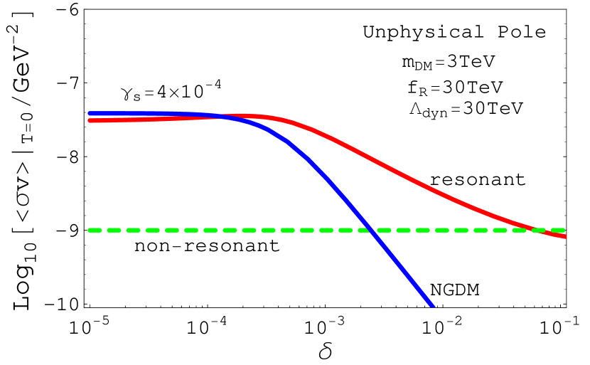
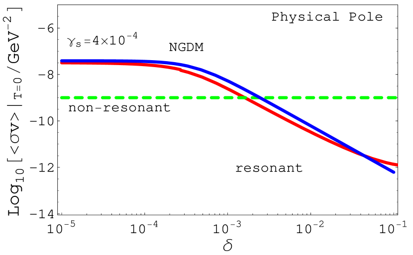
Figure 1: Left) The $\delta$ dependence of the required annihilation cross section at zero temperature from the observed dark matter density in the case of the unphysical pole (red line) for $\gamma_{s}=4\times 10^{-4}$. $m_{\phi}=3$ TeV, $\Lambda_{\rm dyn}=30$ TeV and $f_{R}=30$ TeV, which corresponds to The green line shows the required annihilation cross section in the usual thermal history. The blue line shows the predicted annihilation cross section for $m_{\phi}=3$ TeV, $\Lambda_{\rm dyn}=30$ TeV and $f_{R}=30$ TeV, which corresponds to $\gamma_{s}=4\times 10^{-4}$. Right) The required annihilation cross section in the case of the physical pole. In the figures, we have assumed $x_{f}=30$.

In Fig. 1, we showed the comparison between the predicted and the required cross sections for the unphysical pole for a given parameter set (Left). Here, we numerically solved the Boltzmann equation of the dark matter density. The figure shows that the predicted cross section satisfy the required value at $\delta\simeq 10^{-4}$ for $\Lambda_{\rm dyn}=f_{R}=30$ TeV. For larger values of $\Lambda_{\rm dyn}$ and $f_{R}$, the predicted cross section is always smaller than the required one.

With the above constraint on $\Lambda_{\rm dyn}$ and $f_{R}$, we may derive an upper bound on the effective boost factor in the Breit–Wigner enhancement in the present model. The effective boost factor is given by,

$${\rm BF}=\frac{x_{b}}{x_{f}},$$ (54)

and, for a give value of $\gamma_{s}$, the factor is constraint from above by,

$${\rm BF}\lesssim\frac{1}{x_{f}\,\pi\,\gamma_{s}}=\frac{8f_{R}^{2}}{x_{f}\,m_{\phi}^{2}}\simeq 30\times\left(\frac{30}{x_{f}}\right)\left(\frac{f_{R}}{30\,{\rm TeV}}\right)^{2}\left(\frac{3\,{\rm TeV}}{m_{\phi}}\right)^{2}.$$ (55)

As a result, we found that the effective boost factor cannot be significantly larger than $O(10)$ in this Nambu-Goldstone dark matter model.

Second, we consider the case with the physical pole, $\delta<0$. In this case, both the predicted and the required cross section decreases in $\delta^{-2}$ in a region of $|\delta|>\gamma_{s}$. This means that the predicted cross section satisfies the required value only for a special value of $\Lambda_{\rm dyn}$ and $f_{R}$, i.e.

$$f_{R}\sim\,50\,{\rm TeV}\times\left(1+\frac{\Lambda_{\rm dyn}^{2}}{2f_{R}^{2}}\right)^{-1}.$$ (56)

Inversely, once $\Lambda_{\rm dyn}$ and $f_{R}$ take these values, the predicted dark matter density is consistent with observation for a wide range of $\delta$. In the right panel of Fig. 1, we compared the predicted and the required cross sections. The figure shows that the predicted cross section is consistent with the required cross section in a wide range of $\delta$ for $\Lambda_{\rm dyn}\simeq f_{R}\simeq 30$ TeV.

Put it altogether, the both scenarios require the dynamical scale and the decay constant around $\Lambda_{\rm dyn}\simeq f_{R}\simeq 30$ TeV. From the analysis in the previous section II, these leads to the SUSY breaking scale $F\simeq\lambda^{1/2}\times 30$ TeV. It should be noted, however, that there are $O(1)$ ambiguities associated with the strong dynamics to relate the dynamical scale and the SUSY breaking scale, and hence, the SUSY breaking scale can be slightly different from this naive expectation.

III Cosmic Ray Spectra in Nambu-Goldstone Dark Matter

In this section, we discuss the cosmic ray spectra in the Nambu-Goldstone dark matter scenario. As we have seen, the right amount of the dark matter density is achieved by the annihilation process via the flaton resonance in the early universe. The cosmic ray spectra, on the other hand, depend on how the dark matters behave at the later time of the universe. In the Nambu-Goldstone dark matter scenario, we have two options for the behaviors at the later time. One option is the scenario with the enhanced annihilation and the other is the decaying dark matter. In the case of the annihilating dark matter, the annihilation cross section at the later universe is important. As we have seen, the unphysical flaton pole results in the Breit-Wigner enhancement, which greatly reduces the necessity of the astrophysical boost of the annihilation cross section. In the case of the decaying dark matter, the cosmic ray spectra can be explained regardless of the annihilation cross section, and hence, scenario works well for both the physical and unphysical pole scenarios.

In the followings, we consider both options. As we will see, both options can fit the observed positron/electron spectrum. We further discuss the distinctive prediction on the gamma-ray spectrum, which comes from the finite annihilation/decay rates into the SSM particles.

III.0.1 The electron/positron excesses from the Nambu-Goldstone dark matter

We first consider the electron/positron spectra from the decay/annihilation of the Nambu-Goldstone dark matter with the final states consist of a pair of the R-axions which subsequently decay into pairs of electrons or muons. The detailed parameter sets used for the decay/annihilation of the dark matter are given in Table 1.

Table 1: Setup of the DM decay and annihilation

Mode	$m_{\rm DM}$	$m_{a}$	Decay of $a$	Lifetime/Boost factor
Decay	5 TeV	250 MeV	$\mu^{+}\mu^{-}$	$1.5\times 10^{26}$ sec
Decay	1.5 TeV	5 MeV	$e^{+}e^{-}$	$5\times 10^{26}$ sec
Annihilation	2.5 TeV	250 MeV	$\mu^{+}\mu^{-}$	1500
Annihilation	750 GeV	5 MeV	$e^{+}e-$	150

In Fig. 2, we show the predicted positron fraction (left) and the electron plus positron total flux (right). For the analysis on the propagation of the cosmic ray in the galaxy, we adopt the same set-up in Ref. Shirai:2009kh based on Refs. Hisano:2005ec ; Ibarra:2008qg , namely the MED diffusion model Delahaye:2007fr and the NFW dark matter profile Navarro:1996gj . As for the electron and positron background, we borrowed the estimation given in Refs. Moskalenko:1997gh ; Baltz:1998xv , with a normalization factor $k_{\rm bg}=0.65$. In the analysis of the positron fraction, we have taken into account the solar modulation effect in the current solar cycle Baltz:1998xv , which affects the fraction in $E\lesssim 10$ GeV. The figures show that the excesses observed in the PAMELA and FERMI experiments are nicely fitted by both the annihilation/decay scenario with either four electron or four muon final states.

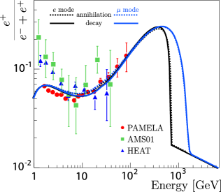
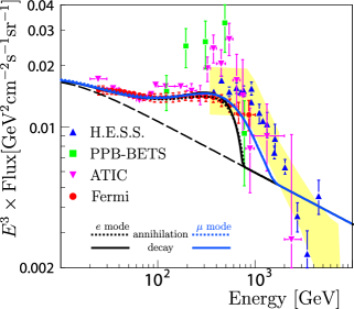
(a) (b)

Figure 2: Cosmic ray signals in the present model. (a): positron fraction with experimental data Adriani:2008zr ; Aguilar:2007yf ; Barwick:1997ig . (b): positron and electron fluxes with experimental data Abdo:2009zk ; Collaboration:2008aaa ; Chang:2008zz ; Torii:2008xu . The yellow zone shows a systematic error and the dashed line shows the background flux.

III.0.2 Flaton decays into SSM particles

In the above analysis, so far, we have considered that the dark matters mainly annihilate/decay into pairs of R-axions which eventually decay into muon or electron pairs. In the Nambu-Goldstone dark matter scenario, however, the interactions between the flaton and the SSM fields are not arbitrary but are fixed for a given gauge mediation mechanism. Thus, in the Nambu-Goldstone dark matter scenario, the SSM final states of the dark matter annihilation/decay are definitely determined for a given gauge mediation model, which gives the model a distinctive prediction on the gamma-ray spectrum.

The decay modes of the flaton into the SSM particles are given as follows. Since we are assuming the models with gauge mediation throughout the paper, the interactions between the flaton and the SSM fields are obtained along with the gauge mediation effects. For example, the effective coupling between the flaton and the gauginos is given by a Yukawa interaction;

$${\cal L}_{\rm eff}\simeq\frac{1}{2}\,\frac{\partial m_{i}}{\partial s}\,s\,\lambda^{i}\lambda^{i}+h.c.,$$ (57)

where $m_{i}$ denotes the gaugino mass and $i$ runs the SSM gauge groups. For example, in a class of the so-called minimal gauge mediation Giudice:1998bp , we obtain,

$$\frac{\partial m_{i}}{\partial s}=\frac{m_{i}}{f_{R}}.$$ (58)

In generic gauge mediation models, it is expected

$$\frac{\partial m_{i}}{\partial s}=c_{g}\frac{m_{i}}{f_{R}},$$ (59)

with an order one coefficient $c_{g}$.

The coupling between the flaton and the sfermions and Higgs bosons are also obtained in a similar way;

$${\cal L}_{\rm eff}=\left.\frac{\partial m_{\tilde{f}}^{2}}{\partial s}\right|_{s=0}\times\,s\,\tilde{f}\tilde{f},$$ (60)

and the model dependent coefficient ${\partial m_{\tilde{f}}^{2}}/{\partial s}$ is again given by,

$$\left.\frac{\partial m_{\tilde{f}}^{2}}{\partial s}\right|_{s=0}=\frac{m_{\tilde{f}}^{2}}{f_{R}},$$ (61)

for the minimal gauge mediation model.

With these interactions, the flaton decays into a pair of the SSM particles. For instance, the decay rate into a pair of the gluinos are given by

$$\Gamma_{s\to\tilde{g}\tilde{g}}\simeq\frac{c_{g}^{2}}{4\pi}\left(\frac{m_{\tilde{g}}}{m_{s}}\right)^{2}\frac{m_{s}^{3}}{f_{R}^{2}}\ .$$ (62)

Thus, when the gluino mass is close to that of the flaton, the branching ratio of the flaton into the gluino pairs can be sizable, which gives a non-trivial contribution to the gamma-ray spectrum.

In the rest of this section, we demonstrate how the SSM modes affect the cosmic gamma-ray spectrum by concentrating on the effects of the sizable gluino branching fraction and take the gluino branching ratio,

$${\rm Br}_{\tilde{g}}=\frac{\Gamma_{s\to\tilde{g}\tilde{g}}}{\Gamma_{s\to aa}}=8c_{g}^{2}\left(\frac{m_{\tilde{g}}}{m_{s}}\right)^{2}\simeq 5.6\times 10^{-2}\times c_{g}^{2}\,\left(\frac{m_{\tilde{g}}}{500\,{\rm GeV}}\right)^{2}\left(\frac{6\,{\rm TeV}}{m_{s}}\right)^{2}\ ,$$ (63)

as a free parameter, which we assume is typically below 10 %. The following analysis can be extended straightforwardly to more detailed analysis on model by model basis for a given gauge mediation mechanism, although we do not peruse in this study.

III.0.3 Gamma-ray and antiproton spectrum with a gluino mode

The gamma-ray signals come from the final state radiation (FSR), inverse Compton scattering (ICS) and the fragmentations of the final states of the decay/annihilation of the dark matter. Especially, in the present model, the contribution from the final states with gluinos has characteristic feature in high-energy region. (As for the FSR and ICS contribution, see Refs. Bergstrom:2008ag ; Mardon:2009gw and Cirelli:2009vg ; Ishiwata:2009dk , respectively)

In this study, we concentrate on the gamma-ray signal from the fragmentation of the gluino final states. As a demonstration, we assume that the branching ratio to the gluinos of the dark matter decay/annihilation is 5 %. Notice that the gamma-ray signal also depends on the decay mode of the gluino. Here, we assume that the sfermions are heavier than the gauginos, and consider two cases with $m_{\tilde{\chi}^{0}_{1}}=100$ GeV and $450$ GeV, while the gluino mass is fixed to $m_{\tilde{g}}=500$ GeV. For simplicity, we further assume the case that the gluino decays into only light quark pair $q,\bar{q}$ and the neutralino $\tilde{\chi}^{0}_{1}$, and the neutralino $\tilde{\chi}^{0}_{1}$ decays into a gravitino and photon.

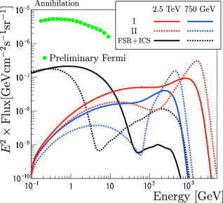
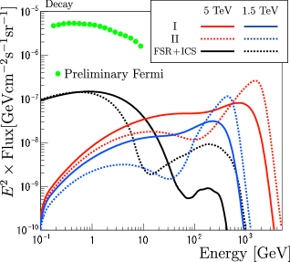
(a) Annihilation (b) Decay

Figure 3: Gamma-ray signals in the present model with experimental data ($0^{\circ}\leq\ell\leq 360^{\circ},~{}10^{\circ}\leq|b|\leq 20^{\circ}$) Porter:2009sg . I and II represent the SSM spectrum where $m_{\tilde{\chi}^{0}_{1}}=100$ GeV and 450 GeV, respectively. FSR+ICS represents the contributions of the FSR and ICS of the electron and positron cosmic ray.

In Fig. 3, the gamma-ray fluxes are shown. To estimate the fluxes, we have used the NFW profile and averaged the halo signal over the region $0^{\circ}\leq\ell\leq 360^{\circ},~{}10^{\circ}\leq|b|\leq 20^{\circ}$ For the annihilation case, we only include the halo component. In Fig. 3, we also show the FSR and ICS contributions from the electron and positron which come from the DM dominant annihilation/decay mode. We estimate the ICS component with the method discussed in Ref. Ishiwata:2009dk , using data of interstellar radiation field provided by the GALPROP collaboration GALPROP , which is based on Ref. Porter:2005qx .

In both cases, the DM signals are consistent with the current experiment data, and anomalous behavior of the gamma ray is expected around the DM mass for the annihilation cases or half for decay. This behavior comes from the hard component from the neutralino $\tilde{\chi}^{0}_{1}$ decay.

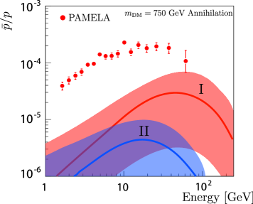
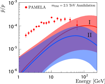
(a) Annihilation $m_{\rm DM}=750$ GeV. (b) Annihilation $m_{\rm DM}=750$ GeV.

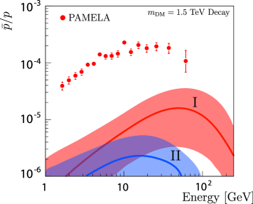
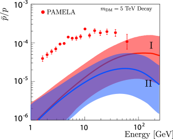
(c) Decay $m_{\rm DM}=1500$ GeV. (d) Decay $m_{\rm DM}=5000$ GeV.

Figure 4: Antiproton signals in the present model with experimental data Adriani:2008zq . I and II represent the SSM spectrum where $m_{\tilde{\chi}^{0}_{1}}=100$ GeV and 450 GeV, respectively.

The gluino final states also raise the antiproton signal, which is severely constrained by the PAMELA experiment Adriani:2008zq . In Fig. 4, we show the ratio of antiproton which comes from signal and the background proton. In this analysis, we used the program PYTHIA Sjostrand:2006za to obtain the fragmentation function of the final states into antiprotons. The analysis of the propagation of the antiproton is again based on that used in Ref. Shirai:2009kh . The figure shows that the antiproton flux strongly depends on the diffusion models, and the shaded region corresponds to the dependence on the diffusion model, with upper side of the region corresponds to the diffusion model MAX, under side MIN and the line MED in Ref.  Delahaye:2007fr . The proton background is taken from Ref. Chen:2009gz . The larger antiproton fluxes in the case of “I” reflect the higher energy fractions of the quark pairs in the decay of the gluinos. We see the contradiction between the experiments and the signals in some diffusion models even for the 5 % branching ratio into the gluino final states.

As a result, we see that the antiproton flux provides very strong constraint on the model. For example, in the minimal gauge mediation, the branching fraction into the gluino final states are solely determined by the masses of the dark matter and the gluino, i.e. $c_{g}=1$ in Eq. (63). Thus, the strict constraint on the branching ratio leads to a strict constraint on the mass of the gluino which is an important parameter for the SUSY search at the coming LHC experiments. Therefore, the Nambu-Goldstone dark matter scenario can be investigated with the interplay between the cosmic-ray experiments as well as the direct SUSY search at the LHC experiment.

References

- (1) O. Adriani et al. [PAMELA Collaboration], Nature 458, 607 (2009) [arXiv:0810.4995 [astro-ph]].
- (2) J. Chang et al., Nature 456, 362 (2008).
- (3) S. Torii et al., arXiv:0809.0760 [astro-ph].
- (4) A. A. Abdo et al. [The Fermi LAT Collaboration], arXiv:0905.0025 [astro-ph.HE].
- (5) For a review, see, e.g., L. Bergstrom, arXiv:0903.4849 [hep-ph] and references therein.
- (6) H. Murayama, talk at 2009 APS April Meeting, May 3, 2009, Denver, Colorado.
- (7) L. Bergstrom, J. Edsjo and G. Zaharijas, arXiv:0905.0333 [astro-ph.HE].
- (8) P. Meade, M. Papucci, A. Strumia and T. Volansky, arXiv:0905.0480 [hep-ph].
- (9) N. Arkani-Hamed, D. P. Finkbeiner, T. R. Slatyer and N. Weiner, Phys. Rev. D 79, 015014 (2009) [arXiv:0810.0713 [hep-ph]].
- (10) Y. Nomura and J. Thaler, arXiv:0810.5397 [hep-ph].
- (11) See, e.g., H. Murayama, arXiv:0704.2276 [hep-ph].
- (12) S. Shirai, F. Takahashi and T. T. Yanagida, arXiv:0905.0388 [hep-ph].
- (13) C. H. Chen, C. Q. Geng and D. V. Zhuridov, arXiv:0905.0652 [hep-ph].
- (14) M. Ibe, Y. Nakayama, H. Murayama and T. T. Yanagida, JHEP 0904, 087 (2009) [arXiv:0902.2914 [hep-ph]].
- (15) For a review, see, e.g., G. F. Giudice and R. Rattazzi, Phys. Rept. 322, 419 (1999) [arXiv:hep-ph/9801271], and references therein.
- (16) K. I. Izawa and T. Yanagida, Prog. Theor. Phys. 95, 829 (1996) [arXiv:hep-th/9602180]; K. A. Intriligator and S. D. Thomas, Nucl. Phys. B 473, 121 (1996) [arXiv:hep-th/9603158].
- (17) J. Bagger, E. Poppitz and L. Randall, Nucl. Phys. B 426, 3 (1994) [arXiv:hep-ph/9405345].
- (18) H. S. Goh and M. Ibe, arXiv:0810.5773 [hep-ph].
- (19) F. Bergsma et al. [CHARM Collaboration], Phys. Lett. B 157, 458 (1985).
- (20) J. E. Kim, Phys. Rept. 150, 1 (1987).
- (21) M. Dine and J. Mason, Phys. Rev. D 77, 016005 (2008) [arXiv:hep-ph/0611312].
- (22) K. Griest and D. Seckel, Phys. Rev. D 43, 3191 (1991).
- (23) P. Gondolo and G. Gelmini, Nucl. Phys. B 360, 145 (1991).
- (24) E. Komatsu et al. [WMAP Collaboration], arXiv:0803.0547 [astro-ph].
- (25) M. Ibe, H. Murayama and T. T. Yanagida, Phys. Rev. D 79, 095009 (2009) [arXiv:0812.0072 [hep-ph]].
- (26) F. Y. Cyr-Racine, S. Profumo and K. Sigurdson, arXiv:0904.3933 [astro-ph.CO].
- (27) M. Aguilar et al. [AMS-01 Collaboration], Phys. Lett. B 646, 145 (2007) [arXiv:astro-ph/0703154].
- (28) S. W. Barwick et al. [HEAT Collaboration], Astrophys. J. 482, L191 (1997) [arXiv:astro-ph/9703192].
- (29) F. Aharonian et al. [H.E.S.S. Collaboration], Phys. Rev. Lett. 101, 261104 (2008) [arXiv:0811.3894 [astro-ph]]; arXiv:0905.0105 [astro-ph.HE].
- (30) S. Shirai, F. Takahashi and T. T. Yanagida, arXiv:0902.4770 [hep-ph].
- (31) J. Hisano, S. Matsumoto, O. Saito and M. Senami, Phys. Rev. D 73, 055004 (2006) [arXiv:hep-ph/0511118].
- (32) A. Ibarra and D. Tran, JCAP 0807, 002 (2008) [arXiv:0804.4596 [astro-ph]].
- (33) T. Delahaye, R. Lineros, F. Donato, N. Fornengo and P. Salati, Phys. Rev. D 77, 063527 (2008) [arXiv:0712.2312 [astro-ph]].
- (34) J. F. Navarro, C. S. Frenk and S. D. M. White, Astrophys. J. 490, 493 (1997) [arXiv:astro-ph/9611107].
- (35) I. V. Moskalenko and A. W. Strong, Astrophys. J. 493 (1998) 694 [arXiv:astro-ph/9710124].
- (36) E. A. Baltz and J. Edsjo, Phys. Rev. D 59 (1999) 023511 [arXiv:astro-ph/9808243].
- (37) K. I. Izawa, Y. Nomura, K. Tobe and T. Yanagida, Phys. Rev. D 56, 2886 (1997) [arXiv:hep-ph/9705228].
- (38) Y. Nomura and K. Tobe, Phys. Rev. D 58, 055002 (1998) [arXiv:hep-ph/9708377].
- (39) M. Ibe and R. Kitano, Phys. Rev. D 75, 055003 (2007) [arXiv:hep-ph/0611111].
- (40) L. Bergstrom, G. Bertone, T. Bringmann, J. Edsjo and M. Taoso, arXiv:0812.3895 [astro-ph].
- (41) J. Mardon, Y. Nomura and J. Thaler, arXiv:0905.3749 [hep-ph].
- (42) M. Cirelli and P. Panci, arXiv:0904.3830 [astro-ph.CO].
- (43) K. Ishiwata, S. Matsumoto and T. Moroi, arXiv:0905.4593 [astro-ph.CO].
- (44) M. Kawasaki, K. Kohri and K. Nakayama, arXiv:0904.3626 [astro-ph.CO].
- (45) T. A. Porter and f. t. F. Collaboration, arXiv:0907.0294 [astro-ph.HE].
- (46) GALPROP Homepage, http://galprop.stanford.edu/.
- (47) T. A. Porter and A. W. Strong, arXiv:astro-ph/0507119.
- (48) O. Adriani et al., Phys. Rev. Lett. 102, 051101 (2009) [arXiv:0810.4994 [astro-ph]].
- (49) T. Sjostrand, S. Mrenna and P. Skands, JHEP 0605, 026 (2006) [arXiv:hep-ph/0603175].
- (50) C. R. Chen, M. M. Nojiri, S. C. Park, J. Shu and M. Takeuchi, arXiv:0903.1971 [hep-ph].