Perturbation Analysis of Complete Synchronization in Networks of Phase Oscillators

Abstract

The behavior of weakly coupled self-sustained oscillators can often be well described by phase equations. Here we use the paradigm of Kuramoto phase oscillators which are coupled in a network to calculate first and second order corrections to the frequency of the fully synchronized state for nonidentical oscillators. The topology of the underlying coupling network is reflected in the eigenvalues and eigenvectors of the network Laplacian which influence the synchronization frequency in a particular way. They characterize the importance of nodes in a network and the relations between them. Expected values for the synchronization frequency are obtained for oscillators with quenched random frequencies on a class of scale-free random networks and for a Erdős-Rényi random network. We briefly discuss an application of the perturbation theory in the second order to network structural analysis.

I. Introduction

The collective behavior of ensembles of interacting units is one of the main topics in complex system theory. Different parts of a complex system can be identified as subsystems and studied individually, while the interaction between these can lead to emergent properties of the whole system. In particular synchronization, the adjustment of internal timescales in oscillatory systems which interact locally or through a complex network PiRoKurths03 ; OsChanKu07 , is ubiquitous in biological Winfree67 ; Tass99 ; ErmKop84 ; BlasiusStone99 ; KoriMikh04 ; KoriMikh06 and technical applications WiesColStro96 ; SiFaWie93 ; LaKoPeHe06 ; DiAre08 . Recently also chemical reactions with feedback control have been proposed to realize specific interaction topologies BlasiusShow07 ; Show05 . Synchronization can orchestrate macroscopic spatio-temporal periodicity even if the individual units are very different from each other and a simple linear superposition of their output would be incoherent. While this is a desirable effect in many applications, such as coupled Josephson junctions or laser arrays WiesColStro96 ; SiFaWie93 it can also lead to pathological states like epilepsy or Parkinson’s disease Tass99 or it can be disastrous when it occurs in constructions OttStrogatz05 .

The onset of synchronization for very heterogeneous systems has been described as a second order phase transition in the limit of large system sizes Kuramoto75 ; Kuramoto84 . Above a critical coupling strength or below a critical heterogeneity the incoherent state becomes unstable and global collective behavior can be observed Kuramoto84 ; RespOtt05 ; Rosenblum07 . For identical, possibly chaotic, subsystems complete synchronization can be possible FujiYa83 ; PecoCar98 . It is known that the spectral properties of the coupling network play an important role in the transition to synchronization OsChanKu07 ; RespOtt05 and the stability of complete synchronization FujiYa83 ; PecoCar98 . But many studies on synchronization in networks have mainly been concerned with the estimation of a few important eigenvalues of the network Laplacian ChanMottKu05 .

In this paper we study the synchronization frequency in networks of weakly nonidentical, autonomous oscillators with attractive coupling. Under these conditions the Kuramoto phase equations (KPE) Kuramoto84 can be used to describe the system qualitatively and quantitatively. The KPE show a rich collective behavior with transitions from complete desynchronization, where the phases are uniformly distributed, to partial synchronization with a unimodal distribution of phases or even clustering Kuramoto84 ; RespOtt05 ; Rosenblum07 ; ErmChimera08 ; KoriKiss07 ; KoriKiss08 and finally frequency synchronization or phase locking, where the phase difference between any two oscillators is constant.

In systems of identical phase oscillators with attractive coupling complete synchronization is a stable solution of the KPE. We will quantify the frequency heterogeneity of the oscillators and derive a perturbation expansion around the well known synchronization manifold for identical oscillators in powers of the heterogeneity. In analogy to perturbation theory for the continuous, nonlinear Kuramoto Phase Diffusion Equation BlaToe08 , in Sections II and III we will show two approaches which lead to the same first and second order perturbation terms. In random networks, the expected second order perturbation term of the synchronization frequency can be interpreted as a mean value with respect to the spectral density of the network Laplacian. Using a random network model for which the spectral density of the Laplacian is known, we explicitly calculate the expected synchronization frequency in Section IV. We verify out theory by numerical simulations.

The Kuramoto model

Let us briefly review the Kuramoto Phase Equations (KPE) for discretely coupled oscillators Kuramoto75 ; Kuramoto84 . The dynamics of an ensemble of $N$ autonomous oscillators may be given as

$$\dot{\mathbf{X}}_{n}=\mathbf{F}_{n}(\mathbf{X}_{n})+\sum_{m=1}^{N}\mathbf{V}_{nm}(\mathbf{X}_{m},\mathbf{X}_{n})~{},$$ (1)

where $\mathbf{X}_{n}$ defines the state of the oscillator labeled with $n$, the velocity field $\mathbf{F}_{n}$ allows for stable limit cycle oscillations and $\mathbf{V}_{nm}$ describes the coupling between two oscillators depending on their state. In his monograph Kuramoto84 Kuramoto considered the heterogeneity in the oscillators as well as the coupling as a perturbation of a common oscillator dynamics $\mathbf{F}_{n}=\mathbf{F}+\delta\mathbf{F}_{n}$. For this common dynamics one can define a uniformly evolving phase variable $\phi$ in a neighborhood of the limit cycle. The dynamics of the phases $\phi_{n}$ in linear response to the perturbation corresponds to the phase model introduced by Winfree Winfree67

$${\dot{\phi}}_{n}=\omega+\delta\omega_{n}(\phi_{n})+\sum_{m=1}^{N}\mathbf{Z}^{\dagger}(\phi_{n}){~{}}\mathbf{V}_{nm}(\phi_{m},\phi_{n})~{}.$$ (2)

Here $\omega$ is the natural frequency and $\mathbf{Z}$ is called the phase response function of the common oscillator dynamics. If the phase differences change slowly over the time of one oscillation then one can use phase averaging techniques Kuramoto84 ; PiRoKurths03 to obtain effective phases $\vartheta_{n}$ and phase equations which only depend on the phase differences. If we finally assume that the functional form of the coupling between any two oscillators $n$ and $m$ only differs in a coupling constant $A_{nm}$ we obtain the KPEs

$${\dot{\vartheta}}_{n}=\omega_{n}+\sum_{m=1}^{N}A_{nm}~{}g(\vartheta_{m}-\vartheta_{n})~{}.$$ (3)

The phase coupling function $g(\Delta\vartheta)$ is periodic. For diffusive coupling it vanishes at zero. We assume a positive derivative at zero and approximate the coupling function by its lowest Fourier modes as

$$g(\Delta\vartheta)=\sin\Delta\vartheta+\gamma\left(1-\cos\Delta\vartheta\right)~{}.$$ (4)

The parameter $\gamma$ breaks the symmetry of the phase coupling function and can directly be associated with the amplitude dependence of the phase velocity in complex Stuart-Landau oscillators Kuramoto84 , i.e. a third-order nonlinear effect in the normal form of a supercritical Hopf bifurcation also known as nonisochronicity. The effect of nonisochronicity on the ability of a system to synchronize and on the formation of spatio-temporal patterns has been noted early on Sakaguchi88 and again stressed recently ErmChimera08 ; BlaToe05 ; Blasius05 whereas it is often disregarded in favor of analytic simplicity Kuramoto84 ; KoriMikh04 ; RespOtt05 .

A fully phase locked state is reached when the oscillators can arrange their phases in a way that due to an exact balance of nonidentical natural frequencies and coupling forces all oscillators have the same synchronization frequency

$$\Omega=\sigma\eta_{n}+\sum_{m=1}^{N}A_{nm}~{}g(\vartheta_{m}-\vartheta_{n})~{}.$$ (5)

The frequencies $\eta_{n}$ in this equation are normalized to have unit variance. Then the heterogeneity of the oscillators is quantified by the variance $\textnormal{var}(\omega)=\sigma^{2}$ of the natural frequencies in the system. The mean frequency $\bar{\omega}$ does not necessarily depend on the heterogeneity $\sigma$ but here we choose a co-rotating frame of reference where $\bar{\omega}=\sigma\bar{\eta}$. For identical oscillators ($\sigma=0$) complete synchronization with identical phases $\vartheta^{(0)}_{n}=\vartheta^{(0)}_{m}$ for all $n$ and $m$, and synchronization frequency $\Omega^{(0)}=0$ is a solution of Eq.(5) with

$$\Omega^{(0)}~{}=~{}0~{}=~{}\sum_{m=1}^{N}A_{nm}~{}g(\vartheta^{(0)}_{m}-\vartheta^{(0)}_{n})~{}.$$ (6)

Stability of the synchronized state

Under some weak conditions on the coupling topology one can show that the state of complete synchronization is stable. But it has been shown recently, that in a heterogeneous coupling network and for large nonisochronicity $\gamma$ the stable state of complete synchronization can co-exist with a dynamical equilibrium of complete desynchronization or partial synchronization ErmChimera08 . Conversely, if the nonisochronicity is not too high and the network is well connected, complete synchronization is the typical result from random initial conditions.

A sufficient condition for the stability of complete synchronization of identical oscillators is that all values $A_{nm}$ are non-negative and the corresponding weighted network is strongly connected, i.e. there exists a path between any two nodes. To see this, one can consider small deviations $\varphi_{n}$ from the synchronized solution. Linearizing Eq. (3) for $\sigma=0$ and small deviations around $\boldsymbol{\vartheta}^{(0)}$ one obtains

$$\dot{\varphi}_{n}=\sum_{m=1}^{N}A_{nm}~{}\left(\varphi_{m}-\varphi_{n}\right)=\sum_{m=1}^{N}L_{nm}~{}\varphi_{m}~{},$$ (7)

with the network Laplacian $\mathbf{L}$ defined as

$$L_{nm}=A_{nm}-\delta_{nm}\sum_{l=1}^{N}A_{nl}~{}.$$ (8)

Since all row sums $\sum_{m}L_{nm}$ are zero at least one eigenvalue $\lambda_{0}$ of the network Laplacian is also zero, corresponding to a constant shift of all phases along the synchronization manifold. If all values $A_{nm}$ are non-negative then it follows from the Gershgorin circle theorem that the network Laplacian has only non-positive eigenvalue real parts $0=\lambda_{0}\geq\textnormal{Re}\lambda_{1}\geq\dots\geq\textnormal{Re}\lambda_{N-1}$, where $N$ is the number of oscillators. Complete synchronization is unique up to a global phase shift, only if the second largest eigenvalue real part $\textnormal{Re}\lambda_{1}$ is strictly smaller than zero.

Associated with the relaxation to synchronization is a diffusion process in the opposite direction of the coupling. If all off-diagonal elements are non-negative, the transposed Laplacian $\mathbf{L}^{\dagger}$ can be viewed as a matrix of transition rates for a master equation $\dot{\mathbf{P}}=\mathbf{L}^{\dagger}\mathbf{P}$ with a probability vector $\mathbf{P}$. The eigenvalue $\lambda_{0}$ is non-degenerate if and only if the stationary probability distribution $\mathbf{P}_{0}$ is unique, i.e. independent of the initial condition. Note, that a strongly connected network of transition rates is sufficient but not necessary for that VanKampen81 . In the following we will assume that $\textnormal{Re}\lambda_{k}<0$ for all $k>0$.

II. Perturbation Approach 1

The algebraic equation Eq.(5) implicitly defines the synchronization frequency and the phases in synchronization (up to global phase shift), even for non-zero heterogeneity. However, a stable phase locked solution of Eq.(5) or any solution at all may not exist. Only for small heterogeneity we can expect that a stable solution exists, that it is close to the solution for identical oscillators ($\sigma=0$) and that it can be expanded in powers of $\sigma$ as

$$\boldsymbol{\vartheta} = \boldsymbol{\vartheta}^{(0)}+\sigma\boldsymbol{\vartheta}^{(1)}+\sigma^{2}\boldsymbol{\vartheta}^{(2)}+~{}O(\sigma^{3})~{},$$

$$\Omega = \sigma\Omega^{(1)}+\sigma^{2}\Omega^{(2)}+~{}O(\sigma^{3})~{}.$$

In this section we follow closely the procedure outlined in BlaToe08 to derive the perturbation expansion of the Kuramoto Phase Equations in synchronization Eq.(5). We directly insert the ansatz Eq.(II. Perturbation Approach 1) into Eq.(5), use a Taylor expansion of the coupling function around zero and regroup the terms according to powers of $\sigma$. This procedure requires sorting of infinite summations and some careful consideration of the index limits. It is shown in detail in the Appendix A. However, the result takes a simple form in vector notation

$$\Omega^{(l)}\mathbf{1}=\left(\mathbf{L}\boldsymbol{\vartheta}^{(l)}+\mathbf{b}^{(l)}\right)~{}.$$ (10)

Here $\Omega^{(l)}$ is the $l^{\textnormal{th}}$ order perturbation term of $\Omega$ in Eq.(II. Perturbation Approach 1), the vector $\boldsymbol{\vartheta}^{(l)}$ is the corresponding perturbation term for the phases in synchronization, $\mathbf{1}$ is a constant vector with unity entries, the matrix $\mathbf{L}$ is the Laplacian of the network, as defined in Equation Eq.(8) and $\mathbf{b}^{(l)}$ is a vector which depends nonlinearly on all perturbation terms of order lower than $l$ (see Eqs. (14)-(16)). Equation (10) can thus be solved iteratively for each order of perturbation. In practice, while the amplitude of the terms $\mathbf{b}^{(l)}$ is as small as $O(\sigma^{l})$, the analytic expression and the expense for its calculation blows up quickly.

Let us consider a complete, orthonormal set of left and right eigenvectors $\mathbf{P}_{k}$ and $\mathbf{p}_{k}$ of the network Laplacian with

$$\mathbf{L}\mathbf{p}_{k}=\lambda_{k}\mathbf{p}_{k}~{}, \quad\mathbf{L}^{\dagger}\mathbf{P}_{k}=\lambda_{k}^{*}\mathbf{P}_{k}~{},$$

$$\mathbf{P}_{k}^{\dagger}{~{}}\mathbf{p}_{k^{\prime}}=\delta_{kk^{\prime}}~{}, \quad\sum_{k=0}^{N-1}\mathbf{p}_{k}\mathbf{P}_{k}^{\dagger}=\mathbb{I}~{},$$

and in particular

$$\mathbf{p}_{0}=\mathbf{1}\quad\textnormal{and}\quad\mathbf{1}^{\dagger}{~{}}\mathbf{P}_{0}=1~{}.$$ (12)

The left eigenvector $\mathbf{P}_{0}$, which is the stationary solution of the master equation $\dot{\mathbf{P}}=\mathbf{L}^{\dagger}\mathbf{P}$, assigns a weight to each node of the network KoriAraiKura09 . The solution of Equation (10) is

$$\Omega^{(l)} = \mathbf{P}_{0}^{\dagger}{~{}}\mathbf{b}^{(l)}~{},$$

$$\boldsymbol{\vartheta}^{(l)} = -\sum_{k\neq 0}\frac{\left(\mathbf{P}_{k}^{\dagger}{~{}}\mathbf{b}^{(l)}\right)}{\lambda_{k}}\mathbf{p}_{k}~{}.$$

Using the short notations $g^{\prime\prime}_{0}=g^{\prime\prime}(0)$, $g^{\prime\prime\prime}_{0}=g^{\prime\prime\prime}(0)$ and $\vartheta_{mn}^{(l)}=\vartheta_{m}^{(l)}-\vartheta_{n}^{(l)}$ the first three vectors $\mathbf{b}^{(1)}$, $\mathbf{b}^{(2)}$ and $\mathbf{b}^{(3)}$ are

$$b_{n}^{(1)} = \eta_{n}~{},$$ (14)

$$b_{n}^{(2)} = \sum_{m=1}^{N}A_{nm}\frac{1}{2}g^{\prime\prime}_{0}{\vartheta_{mn}^{(1)}}^{2}~{},$$ (15)

$$b_{n}^{(3)} = \sum_{m=1}^{N}A_{nm}\left(g^{\prime\prime}_{0}\vartheta_{mn}^{(1)}\vartheta_{mn}^{(2)}+\frac{1}{6}g^{\prime\prime\prime}_{0}{\vartheta_{mn}^{(1)}}^{3}\right)~{}.$$ (16)

Equations (II. Perturbation Approach 1)-(16) give the first three perturbation terms of the synchronization frequency and the relative phases in synchronization. In the next section, we will derive the first and the second order terms again, but in a slightly different form which allows for a better analysis.

III. Perturbation Approach 2

The second order correction Eqs. (II. Perturbation Approach 1) and (15) of the synchronization frequency depends on the second derivative $g^{\prime\prime}_{0}=g^{\prime\prime}(0)$ of the phase coupling function at zero. If we are only interested in the first and second order perturbation terms we have the freedom to choose a different coupling function $\tilde{g}(\varphi)$ in the equation Eq.(5) with the same first and second derivative at zero as $g(\varphi)$ which may be more suitable for an analysis. For the continuous Kuramoto Phase Diffusion equations it is known that a non-linear Cole-Hopf transformation $\vartheta=\gamma^{-1}\log p$ changes the equations in synchronization into an eigenvalue problem of a stationary, linear Schrödinger equation Kuramoto84 ; Sakaguchi88 ; BlaToe05 ; BlaToe08 . With the same procedure in mind we will define an auxiliary coupling function $\tilde{g}(\varphi)$ as

$$\tilde{g}(\varphi)~{}=~{}\frac{1}{\gamma}\left(e^{\gamma\varphi}-1\right)~{}=~{}g(\varphi)~{}+~{}O(\varphi^{3})~{}.$$ (17)

After the transformation

$$\vartheta_{n}=\frac{1}{\gamma}\log p_{n}~{},$$ (18)

we can bring equation Eq.(5) with $\tilde{g}(\varphi)$ as coupling function into the form of an eigenvalue problem

$$-E_{0}\mathbf{p}~{}=~{}\gamma\Omega\mathbf{p}~{}=~{}\bigl{[}\gamma\sigma\mathbf{V}_{\eta}+\mathbf{L}\bigr{]}~{}\mathbf{p}~{}=~{}-\mathbf{H}\mathbf{p}~{},$$ (19)

where the vector $\mathbf{p}$ has the entries $p_{n}$, $\mathbf{V}_{\eta}=\textnormal{diag}(\boldsymbol{\eta})$ is the diagonal matrix of frequencies and $\mathbf{L}$ is the network Laplacian (Eq.(8)). This equation has the form of a stationary discrete Schrödinger equation for the ground state of a particle hopping between the vertices of the coupling graph with the on-site potentials $-\eta_{n}$ and ground state energy $E_{0}=-\gamma\Omega$. If the coupling network is symmetric the Hamiltonian $\mathbf{H}$ is symmetric, as well, the left and right eigenvectors are identical and all eigenvalues are real. In this section we will not yet make this simplifying assumption.

The potential $\mathbf{V}_{\eta}$ of random frequencies can be treated as a perturbation of strength $\gamma\sigma$ of the eigenvalue problem for the network Laplacian. Given the eigenvalues and orthonormal left and right eigenfunctions of $\mathbf{L}$ Eq.(II. Perturbation Approach 1) we are looking for the coefficients $E_{0}^{(l)}$ of the expansion

$$-E_{0}~{}=~{}\lambda_{0}~{}-~{}\gamma\sigma E_{0}^{(1)}~{}-~{}\gamma^{2}\sigma^{2}E_{0}^{(2)}~{}-~{}O(\gamma^{3}\sigma^{3})~{}.$$ (20)

Again, we assume that the eigenvalue $\lambda_{0}=0$ of the Laplacian is non-degenerate, so that the ground state is unique up to normalization. Accordingly, the synchronized state is unique up to a constant phase shift. Schrödinger perturbation theory, modified to allow for asymmetric operators gives the expressions

$$-E_{0}^{(1)} = \left(\mathbf{P_{0}}^{\dagger}{~{}}\mathbf{V}_{\eta}\mathbf{p}_{0}\right)~{},$$

$$-E_{0}^{(2)} = \sum_{k\neq 0}\frac{\left(\mathbf{P}_{0}^{\dagger}{~{}}\mathbf{V}_{\eta}\mathbf{p}_{k}\right)\left(\mathbf{P}_{k}^{\dagger}{~{}}\mathbf{V}_{\eta}\mathbf{p}_{0}\right)}{\lambda_{0}-\lambda_{k}}~{}.$$

For the first two coefficients in the perturbation expansion Eq.(II. Perturbation Approach 1) of the synchronization frequency $\Omega$ we find

$$\Omega^{(1)} = \mathbf{P}_{0}^{\dagger}{~{}}\boldsymbol{\eta}~{},$$

$$\Omega^{(2)} = -\gamma\sum_{k\neq 0}\frac{\left(\mathbf{P}_{0}^{\dagger}{~{}}\mathbf{V}_{\eta}\mathbf{p}_{k}\right)\left(\mathbf{P}_{k}^{\dagger}{~{}}\mathbf{V}_{\eta}\mathbf{p}_{0}\right)}{\lambda_{k}}~{}.$$

The first term is the weighted average of the frequencies with respect to the stationary probability distribution of the master equation $\dot{\mathbf{P}}=\mathbf{L}^{\dagger}\mathbf{P}$ with the transposed network Laplacian as matrix of transition rates. In the second expression we have used $\Omega^{(2)}=-\gamma E_{0}^{(2)}$ and $\lambda_{0}=0$. Equation Eq.(III. Perturbation Approach 2) is a more compact form of equations Eqs. (II. Perturbation Approach 1)-(15) combined.

IV. Examples

We can now study the change of the synchronization frequency with respect to oscillator heterogeneity and to the architecture of the coupling network. To find expressions for the expected first and second order response we will consider the ensemble of different realizations of random frequencies and an ensemble of random networks. Let us assume independent, identically distributed random frequencies with $\mathbb{E}\left[\eta_{n}\eta_{m}\right]-\mathbb{E}\left[\eta\right]^{2}=\delta_{nm}$ Then from Eq.(III. Perturbation Approach 2) follows

$$\mathbb{E}\left[\Omega^{(1)}\right] = \mathbb{E}_{\eta}\left[\eta\right]~{},$$

$$\mathbb{E}\left[\Omega^{(2)}\right] = -\gamma~{}\mathbb{E}_{NW}\left[\sum_{k\neq 0}\frac{\left(\mathbf{P}_{k}^{\dagger}{~{}}\mathbf{V}_{\mathbf{P}_{0}}~{}\mathbf{p}_{k}\right)}{\lambda_{k}}\right]~{}.$$

Here $\mathbb{E}_{\eta}$ is the expected value with respect to the frequency distribution and $\mathbb{E}_{NW}$ over the network ensemble. The vectors $\mathbf{P}_{k}$ and $\mathbf{p}_{k}$ in the second equation are left and right eigenvectors of the network Laplacian and $\lambda_{k}\neq 0$ the corresponding eigenvalues. The operator $\mathbf{V}_{\mathbf{P}_{0}}$ is diagonal with the components of $\mathbf{P}_{0}$ on the diagonal. The first order frequency correction is independent of the network architecture while for uncorrelated frequencies the second order perturbation term is determined by the topology of the coupling network and the frequency heterogeneity $\sigma^{2}$. For symmetric coupling $A_{nm}=A_{mn}$ the left eigenvector $\mathbf{P}_{0}$ is given by $N^{-1}\mathbf{1}$ and in the limit $N\to\infty$ the expected value of $\Omega^{(2)}$ in Eq. (IV. Examples) can be written as

$$\mathbb{E}\left[\Omega^{(2)}\right]~{}=~{}\gamma\int~{}\rho(\lambda)~{}\frac{1}{\lambda}~{}d\lambda~{},$$ (24)

where $\rho(\lambda)$ is the Laplacian spectral density of the random network ensemble.

The integral Eq. (24) has been studied in the different context of vibrational thermodynamic stability for networks of linear springs, modelling complex molecules BuCaFoVu02 . Whether the integral is finite depends on the spectral dimension $d$ of the network, defined by the limit behavior of $\rho(\lambda)\sim\lambda^{\frac{d}{2}-1}$ for $\lambda\to 0$, a suitable generalization of the Euclidean dimension for regular lattices to geometrically disordered structures OrAl82 . For networks with spectral dimension $d>2$ larger than two, the integral in Eq. (24) is finite. In BuCaFoVu02 the authors study the case of a Sierpinski gasket which is a fractal graph for which the Laplacian spectrum can be calculated analytically and the spectral dimension is lower than two. In BlaToe08 we study regular topologies for which the Fourier spectral decomposition is known and we also find the lower critical dimension $d=2$. For ensembles of random graphs in general, it is a complicated task to find analytic expressions for the spectral density. Approximations of the spectral density of matrices associated with complex random networks, such as the Wigner semicircle law, are usually only available in the limit of dense networks, where the mean degree is much larger than one.

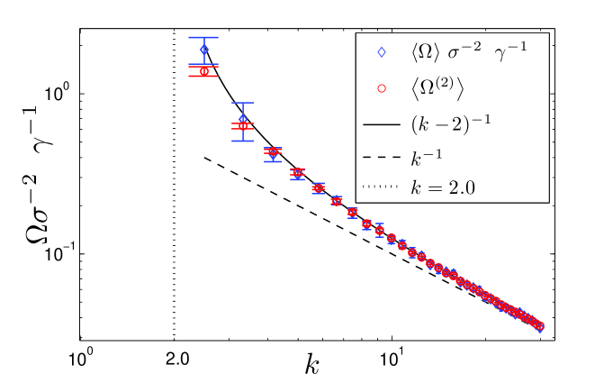
Figure 1: (color online) Frequency shift in undirected, random networks of size $N=400$ with Poissonian degree distribution and given mean degree $k$. The mean degree must be larger than $k_{cr}=2$ for an infinite random tree network. The frequency shift could be measured precisely by enforcing a zero mean frequency $\bar{\omega}=0$. Random frequencies were drawn from a uniform distribution of standard deviation $\sigma=10^{-1}$. From an ensemble of 10 realizations we show the mean network synchronization frequency divided by variance $\sigma^{2}$ and nonisochronicity $\gamma$ (blue diamonds, Newton Method, $\gamma=1.0$), the predicted second order term $\langle\Omega^{(2)}\rangle$ from equation Eq.(IV. Examples) and the spectrum of the network Laplacian (red circles), the asymptotic line $k^{-1}$ (dashed line) and the line $(k-2)^{-1}$ (solid line), which describes the actual behavior of the frequency shift even for small mean degrees close to $k_{cr}=2$.

A static scale-free random network model

As an example we will use a recent result for the Laplacian of a static scale-free random network model Kahng01 ; Kahng07 . For this model the coupling strength $A_{nm}=A_{mn}$ between two oscillators is either zero or it is one with the probability $kNw_{n}w_{m}$, where the $w_{n}\sim n^{-1/(\alpha-2)}$ are normalized weights for the nodes $n=1\dots N$, and $k$ is the mean degree of the network. The degree distribution follows a power law with exponent $-\alpha$. In the thermodynamic limit $N\to\infty$ and large $k\gg 1$ the spectral density of the Laplacian Eq.(8) is given Kahng07 as

$$\rho(\lambda) = \left\{\begin{array}[]{l l}(\alpha-1)(-\lambda_{c})^{\alpha-1}~{}(-\lambda)^{-\alpha}&\quad\textnormal{for }\lambda<\lambda_{c}<0~{},\\ 0&\quad\textnormal{otherwise}~{},\end{array}\right.$$ (27)

$$\lambda_{c} = -k(\alpha-2)(\alpha-1)^{-1}~{}.$$

Using this spectral density in equation Eq.(24) we obtain

$$\mathbb{E}\left[\Omega^{(2)}\right]~{}=~{}\gamma\int d\lambda~{}\rho(\lambda)~{}\frac{1}{\lambda}~{}=~{}\gamma k^{-1}\frac{(\alpha-1)^{2}}{\alpha(\alpha-2)}~{}.$$ (29)

Erdős-Rényi model and random tree network limit

The Erdős-Rényi random model REgraph59 is recovered as a special case of the static scale-free random network model in the limit $\alpha\to\infty$ Kahng01 . Then for $k\gg 1$ we find $\mathbb{E}\left[\Omega^{(2)}\right]=\gamma k^{-1}$. One can study the limit of sparse uncorrelated random graphs by removing edges randomly without breaking the network in two components. The mean degree in a single component, undirected graph cannot be smaller than $2(N-1)/N$ for a tree network. Every edge that is removed then breaks the connectivity, creates a new component and thus a new zero eigenvalue of the Laplacian. We expect therefore a divergence of the integral in Eq. (24) for $k\to 2$. We have tested our theory numerically for symmetrically connected random graphs with Poissonian uncorrelated degree distributions and $N=400$ phase oscillators with nonisochronicity $\gamma=1.0$. The frequencies were chosen randomly from a uniform distribution with $\textnormal{var}(\omega)=\sigma^{2}=10^{-2}$. The synchronization frequency $\Omega$ was determined on one hand by solving the algebraic equations Eq.(5) with a Newton method, instead of integrating the KPEs Eq.(3), and on the other hand by using our perturbation approach and the complete eigenvalue spectrum of the network Laplacians. The results can be seen in Fig. (1). One can, indeed, see that the second order perturbation term diverges as $(k-2)^{-1}$ which is consistent with a powerlaw scaling $\mathbb{E}\left[\Omega^{(2)}\right]=\gamma k^{-1}$ for larger mean degrees $k$.

Application to network structure analysis

In order to demonstrate possible applications of this perturbation theory to structural analysis of an unknown coupling network let us now briefly study what information can be gained from a measurement of linear and nonlinear responses to frequency changes of the oscillators. In Timme07 the author presents a method to reconstruct a coupling network from measuring the linear response of the phase differences to linearly independent changes of the natural frequencies. This corresponds to using Eq. (II. Perturbation Approach 1). The coupling network can be identified from the Green’s function $\mathbf{G}$ of the network Laplacian and Eq. (II. Perturbation Approach 1) reads

$$\boldsymbol{\vartheta}^{(1)}=\mathbf{G}\boldsymbol{\eta}~{}.$$ (30)

If the phase differences are not accessible to direct measurement one can in principle also obtain the Green’s function from the second order shift in the synchronization frequency. For a symmetric coupling Eq. (III. Perturbation Approach 2) gives

$$\Omega(\boldsymbol{\omega})=\bar{\omega}+\gamma~{}\frac{1}{N}\boldsymbol{\omega}^{\dagger}\mathbf{G}\boldsymbol{\omega}~{}.$$ (31)

Let $\{\boldsymbol{\omega}^{(\alpha)}\}$ be a basis set of linear independent frequency detunings. Then the Green’s function with respect to this basis can be determined from $N(N+1)/2$ measurements of synchronization frequencies as

$$\Omega\left(\boldsymbol{\omega}^{(\alpha)}+\boldsymbol{\omega}^{(\beta)}\right)-\left(\Omega\left(\boldsymbol{\omega}^{(\alpha)}\right)+\Omega\left(\boldsymbol{\omega}^{(\beta)}\right)\right)=2\gamma\frac{1}{N}~{}\boldsymbol{\omega}^{(\alpha)\dagger}\mathbf{G}\boldsymbol{\omega}^{(\beta)}~{}.$$ (32)

However, due to the number of measurements and the large time scales of a diffusion process the application is limited to very small networks, fast relaxation to the phase locked solution and high precision measurements. The analysis can be extended to nonidentical oscillators and asymmetric coupling.

V. Discussion

We have presented expressions for the first and second order perturbation terms of the synchronization frequency in complex networks of coupled Kuramoto phase oscillators with quenched frequency disorder. The two approaches in Sections II and III give equivalent results, but the second approach, based on a nonlinear approximation of the phase coupling function around zero, extends a well known treatment of the Kuramoto phase equations from continuous media to complex networks Kuramoto84 ; Sakaguchi88 ; BlaToe08 . The results were given in terms of the eigenvalues and eigenvectors of the Laplacian matrix of the coupling network. In a single component with mean degree $k$ of a undirected Erdős-Rényi random coupling network REgraph59 and for oscillators with independent, identically distributed random frequencies $\omega_{n}$ of variance $\sigma^{2}$ and nonisochronicity $\gamma$ the expected synchronization frequency was found to be

$$\mathbb{E}\left[\Omega\right]~{}=~{}\mathbb{E}\left[\omega\right]~{}+~{}\gamma~{}\textnormal{var}(\omega)~{}(k-2)^{-1}~{}+~{}O(\gamma^{2}\sigma^{3})~{}.$$ (33)

While the expected synchronization frequency depends to the first order only on the natural frequencies in the system, the second order correction combines the nonlinearity $\gamma$ of the phase coupling function around zero, the variance of the frequencies and the mean degree of the coupling network in a simple way.

The explicit connection between synchronization frequency, natural frequencies and network structure in the Eq. (III. Perturbation Approach 2) makes it in principle possible to infer information of either property from a measurement or the knowledge of the other properties. Network reconstruction by observing the linear response to a frequency detuning has already been proposed and successfully applied Timme07 . An analogous approach using frequency measurements instead of phase differences may be constructed based on the results of this paper.

This work was supported by the German DFG through the project SfB555 and the Japanese JSPS.

Appendix A

Given the Kuramoto phase equations in synchronization

$$\Omega=\sigma\eta_{n}+\sum_{m=1}^{N}A_{nm}~{}g(\vartheta_{m}-\vartheta_{n})~{},$$ (34)

and a phase locked solution of the KPEs for identical oscillators

$$\Omega^{(0)}=\sum_{m=1}^{N}A_{nm}~{}g(\vartheta^{(0)}_{m}-\vartheta^{(0)}_{n})~{},$$ (35)

we want to derive expressions for the coefficients in the expansion of the synchronization frequency $\Omega$ in powers of the frequency heterogeneity $\sigma$. Let us start by implicitly defining notations for the involved perturbation terms and phase differences

$$\Omega = \Omega^{(0)}+\sum_{l=1}^{\infty}\sigma^{l}~{}\Omega^{(l)}~{},$$ (36)

$$\vartheta_{n} = \vartheta_{n}^{(0)}+\varphi_{n}~{}=~{}\vartheta_{n}^{(0)}+\sum_{l=1}^{\infty}\sigma^{l}~{}\vartheta_{n}^{(l)}~{},$$ (37)

$$\vartheta_{mn} = \vartheta_{m}-\vartheta_{n}~{}=~{}\vartheta_{mn}^{(0)}+\varphi_{mn}~{}=~{}\vartheta_{mn}^{(0)}+\sum_{l=1}\sigma^{l}~{}\vartheta_{mn}^{(l)}~{},$$ (38)

$$\varphi_{mn}^{j} = (\varphi_{m}-\varphi_{n})^{j}=\sum_{l=j}^{\infty}\sigma^{l}~{}\varphi_{mn}^{(j,l)}~{},$$ (39)

$$g_{mn} = g\left(\vartheta_{mn}^{(0)}\right)~{},\qquad g_{mn}^{(j)}=\partial^{j}g_{mn}~{}.$$ (40)

Note that here we do not assume $\boldsymbol{\vartheta}^{(0)}=\textnormal{const}$, $g(0)=0$ or $g_{mn}^{(j)}=g^{(j)}(0)$. It has been pointed out, that even for identical oscillators the homogeneous solution may not be the only synchronized solution of the Kuramoto phase equations Strogatz06 . In certain coupling topologies and for large nonisochronicity the completely synchronized solution can coexist with a dominating chaotic attractor of drifting phases ErmChimera08 . If the network is homogeneous and sufficiently well connected, however, the stable solution of complete synchronization is typical. Therefore we assume $\Omega^{(0)}=g(0)=0$ and $g^{(j)}_{mn}=g^{(j)}(0)$ in the main text of this paper.

The coefficients $\varphi_{mn}^{(j,l)}$ yield the recursion relation

$$\varphi_{mn}^{(j,l)}=\left\{\begin{array}[]{l l}\vartheta_{mn}^{(l)}&~{}~{}\textnormal{for}\quad j=1~{},\\ \sum_{k=1}^{l-1}\vartheta_{mn}^{(k)}\varphi_{mn}^{(j-1,l-k)}&~{}~{}\textnormal{for}\quad j\leq l~{},\\ 0&~{}~{}\textnormal{otherwise}~{}.\end{array}\right.$$ (41)

Inserting Eq.(37) into Eq.(34) we find

$$\Omega = \sigma\eta_{n}+\sum_{m=1}^{N}A_{nm}~{}g_{mn}~{},$$

$$= \Omega^{(0)}+\sigma\eta_{n}+\sum_{m=1}^{N}A_{nm}~{}\sum_{j=1}^{\infty}\frac{1}{j!}g_{mn}^{(j)}\varphi_{mn}^{j}~{},$$

$$= \Omega^{(0)}+\sigma\eta_{n}+\sum_{m=1}^{N}A_{nm}~{}\sum_{j=1}^{\infty}\frac{1}{j!}g_{mn}^{(j)}\sum_{l=j}^{\infty}\sigma^{l}\varphi_{mn}^{(j,l)}~{},$$

$$= \Omega^{(0)}+\sigma\eta_{n}+\sum_{l=1}^{\infty}\sigma^{l}\sum_{j=1}^{l}\sum_{m=1}^{N}A_{nm}~{}\frac{1}{j!}g_{mn}^{(j)}\sum_{k=1}^{l-1}\varphi_{mn}^{(1,k)}\varphi_{mn}^{(j-1,l-k)}~{}.$$

In the second line we have inserted the unperturbed solution Eq.(35) and in the third line we used the expansion Eq.(39) of the powers of $\varphi_{mn}$. Since the leading order of $\varphi_{mn}$ in $\sigma$ is one, the $j$th power has a leading term of order $j$. In the last line the recursion relation (41) was used. If we now collect the nonlinear terms ($j>1$) in a vector $\mathbf{b}^{(l)}$ we can write down this result in a more compact form

$$\Omega-\Omega^{(0)}=\sum_{l=1}\sigma^{l}\Omega^{(l)}=\sum_{l=1}\sigma^{l}\left(\sum_{m=1}^{N}A_{nm}g^{\prime}_{mn}\vartheta_{mn}^{(l)}+b_{n}^{(l)}\right)~{},$$ (43)

or in vector form

$$\Omega^{(l)}\mathbf{1}=\left(\mathbf{L}\boldsymbol{\vartheta}^{(l)}+\mathbf{b}^{(l)}\right)~{},$$ (44)

where $\mathbf{1}$ is a constant vector of unit entries, $\boldsymbol{\vartheta}^{(l)}$ is the vector of perturbative corrections $\vartheta_{n}^{(l)}$ to the phases and $\mathbf{b}^{(l)}$ is a vector which only depends on perturbation terms of order lower than $l$. The matrix $\mathbf{L}$ is the Jacobian

$$L_{nm}=A_{nm}~{}g^{\prime}_{mn}-\delta_{nm}\sum_{l=1}^{N}A_{nl}~{}g^{\prime}_{ln}~{},$$ (45)

or the Laplacian if $g^{\prime}_{mn}$ is a constant. The vectors $\mathbf{b}^{(l)}$ are given by

$$b_{n}^{(1)} = \eta_{n}~{},$$ (46)

$$b_{n}^{(2)} = \sum_{m=1}^{N}A_{nm}~{}\frac{1}{2}g_{mn}^{\prime\prime}{\vartheta_{mn}^{(1)}}^{2}~{},$$ (47)

$$b_{n}^{(3)} = \sum_{m=1}^{N}A_{nm}\left(g_{mn}^{\prime\prime}\vartheta_{mn}^{(1)}\vartheta_{mn}^{(2)}+\frac{1}{6}g_{mn}^{\prime\prime\prime}{\vartheta_{mn}^{(1)}}^{3}\right)~{},$$ (48)

and in general for $l>1$

$$b_{n}^{(l>1)}=\sum_{j=2}^{l}\sum_{m=1}^{N}A_{nm}\frac{1}{j!}g_{mn}^{(j)}\sum_{k=1}^{l-1}\vartheta_{mn}^{(k)}\varphi_{mn}^{(j-1,l-k)}~{}.$$ (49)

Equation Eq.(44) can be solved iteratively for each perturbation order. Let us consider a complete, orthonormal set of left and right eigenvectors $\mathbf{P}_{k}$ and $\mathbf{p}_{k}$ of the Jacobian with

$$\mathbf{L}\mathbf{p}_{k}=\lambda_{k}\mathbf{p}_{k}~{}, \quad\mathbf{L}^{\dagger}\mathbf{P}_{k}=\lambda_{k}^{*}\mathbf{P}_{k}~{},$$

$$\mathbf{P}_{k}^{\dagger}{~{}}\mathbf{p}_{k^{\prime}}=\delta_{kk^{\prime}}~{}, \quad\sum_{k=0}^{N-1}\mathbf{p}_{k}\mathbf{P}_{k}^{\dagger}=\mathbb{I}~{},$$

and in particular

$$\mathbf{p}_{0}=\mathbf{1}~{},\qquad\mathbf{1}^{\dagger}{~{}}\mathbf{P}_{0}=1~{}.$$ (51)

We can now define the projectors

$$\mathbb{P}_{0}=\mathbf{p}_{0}\mathbf{P}_{0}^{\dagger}~{},\qquad\mathbb{Q}_{0}=\mathbb{I}-\mathbb{P}_{0}~{}.$$ (52)

The operation $\mathbb{P}_{0}\mathbf{x}$ projects to a constant vector where all entries are equal to the weighted average $\langle x\rangle_{\mathbf{P}_{0}}$ and $\mathbb{Q}_{0}$ removes this average from the components of a vector. Applying these projectors to Equation Eq.(44) we obtain

$$\Omega^{(l)} = \mathbf{P}_{0}^{\dagger}{~{}}\mathbf{b}^{(l)}~{},$$ (53)

$$0 = \mathbf{L}\boldsymbol{\vartheta}^{(l)}+\mathbb{Q}_{0}\mathbf{b}^{(l)}~{}.$$ (54)

The last equation is solved for $\boldsymbol{\vartheta}^{(l)}$ up to an arbitrary global phase shift by

$$\boldsymbol{\vartheta}^{(l)}=-\sum_{k\neq 0}\frac{\left(\mathbf{P}_{k}^{\dagger}{~{}}\mathbf{b}^{(l)}\right)}{\lambda_{k}}\mathbf{p}_{k}~{}.$$ (55)

References

- (1) A. Pikovsky, M. Rosenblum and J. Kurths, Synchronization: A Universal Concept in Nonlinear Sciences, (Cambridge University Press, 2003).
- (2) G. V. Osipov, J. Kurths and C. Zhou, Synchronization in Oscillatory Networks, Springer Series in Synergetics, (Springer-Verlag Gmbh, 2007).
- (3) A. T. Winfree, Biological rhythms and the behavior of populations of coupled oscillators, J. Th. Bio. 16, 1 pp. 15-42 (1967)
- (4) P. A. Tass, Phase Resetting in Medicine and Biology, (Springer-Verlag Berlin and Heidelberg, 1999).
- (5) G. B. Ermentrout and N. Kopell, Frequency plateaus in a chain of weakly coupled oscillators, I. SIAM J. Math. Anal. 15, 215-237 (1984)
- (6) B. Blasius and A. Huppert and L. Stone Complex dynamics and phase synchronization in spatially extended ecological systems Nature 399, 354-359 (1999)
- (7) H. Kori and A. S. Mikhailov, Entrainment of Randomly Coupled Oscillator Networks by a Pacemaker, Phys. Rev. Lett. 93, 254101 (2004)
- (8) H. Kori and A. S. Mikhailov, Strong effects of network architecture in the entrainment of coupled oscillator systems Phys. Rev. E 74, 066115 (2006)
- (9) K. Wiesenfeld, P. Colet, and S. H. Strogatz, Synchronization transitions in a disordered Josephson series array, Phys. Rev. Lett., 76, 404, (1996).
- (10) M. Silber, L. Fabiny and K. Wiesenfeld, Stability results for in-phase and splay-phase states of solid-state laser arrays, J. Opt. Soc. Am. B 10:1121 (1993).
- (11) S. Lämmer, H. Kori, K. Peters and D. Helbing, Decentralised control of material or traffic flows in networks using phase-synchronisation, Physica A 363, 1, (2006).
- (12) A. Diaz-Guilera and A. Arenas, Phase patterns of coupled oscillators with application to wireless communication, ”Bio-Inspired Computing and Communication” Lect. Notes Comp. Sci. (in press, 2008)
- (13) O.-U. Kheowan and E. Mihaliuk and B. Blasius and I. Sendina-Nadal and K. Showalter Wave mediated synchronization of nonuniform oscillatory media Phys. Rev. Lett. 98, 074101 (2007)
- (14) M. Tinsley, J. Cui, F. V. Chirila, A. Taylor, S. Zhong and K. Showalter, Spatiotemporal Networks in Addressable Excitable Media, Phys. Rev. Lett. 95, 038306 (2005)
- (15) S. H. Strogatz, D. M. Abrams, A. McRobie, B. Eckhardt and E. Ott, Theoretical mechanics : Crowd synchrony on the millennium bridge, Nature 438 p.43-44, 2005.
- (16) Y. Kuramoto, Self-entrainment of a population of coupled nonlinear oscillators Lect. N. Phys. vol. 39, pp. 420-422 (Springer, New York, 1975)
- (17) Y. Kuramoto Chemical oscillations, waves and turbulence, (Springer, Berlin, 1984).
- (18) J. G. Restrepo, E. Ott, and B. R. Hunt, Onset of synchronization in large networks of coupled oscillators, Phys. Rev. E 71, 036151 (2005)
- (19) M. Rosenblum and A. Pikovsky, Self-organized quasiperiodicity in oscillator ensembles with global nonlinear coupling, Phys. Rev. Lett. 98, 064101 (2007)
- (20) H. Fujisaka and T. Yamada, Stability of Synchronized Motion in Coupled-Oscillator Systems, Prog. Theo. Phys. 69, 1 (1983)
- (21) L. M. Pecora and T. L. Carroll, Master stability functions for synchronized coupled systems, Phys. Rev. Lett. 80 2109 (1998)
- (22) A. E. Motter, C. Zhou, J. Kurths, Enhancing complex-network synchronization, Europhys. Lett. 69, 334 (2005)
- (23) T.-W. Ko and G. B. Ermentrout, Bistability between synchrony and incoherence in limit-cycle oscillators with coupling strength inhomogeneity, Phys. Rev. E 78, 026210 (2008)
- (24) I. Z. Kiss, C. G. Rusin, H. Kori and J. L. Hudson, Engineering complex dynamical structures: Sequential patterns and desynchronization, Science, 316 no.5833 p.1886 - 1889 (2007).
- (25) H. Kori, C. G. Rusin, I. Z. Kiss, and J. L. Hudson, Synchronization Engineering: Theoretical Framework and Application to Dynamical Clustering Chaos 18, 026111 (2008)
- (26) R. Toenjes and B. Blasius, Perturbation Analysis of the Kuramoto Phase Diffusion Equation Subject to Quenched Frequency Disorder, Phys. Rev. E 79, 016112 (2009)
- (27) H. Sakaguchi, S. Shinomoto and Y. Kuramoto, Mutual Entrainment in Oscillator Lattices with Nonvariational Type Interaction, Prog. of Theor. Phys. 79, 1069 (1988).
- (28) B. Blasius, R. Tönjes, Quasiregular Concentric Waves in Heterogeneous Lattices of Coupled Oscillators, Phys. Rev. Lett. 95, 084101 (2005)
- (29) B. Blasius Anomalous phase synchronization in two asymmetrically coupled oscillators in the presence of noise Phys. Rev. E 72, 066216 (2005)
- (30) N. G. Van Kampen, Stochastic Processes in Physics and Chemistry, (North-Holland Publishing Co, 3rd edition (2007)).
- (31) H. Kori, Y. Kawamura, H. Nakao, K. Arai and Y. Kuramoto, Collective dynamical response of coupled oscillators with any network structure unpublished (arXiv:0812.0118v1)
- (32) R. Burioni, D. Cassi, M.P. Fontana and A. Vulpiani, Vibrational thermodynamic instability of recursive networks, Chaos 16, 015103 (2006).
- (33) S. Alexander, R.L. Orbach, Density of states on fractals: fractons, J. Physique Lett. 43, p.625-631 (1982)
- (34) K.-I. Goh, B. Kahng and D. Kim, Universal Behavior of Load Distribution in Scale-Free Networks, Phys. Rev. Lett. 87, 278701 (2001).
- (35) D. Kim and B. Kahng, Spectral densities of scale-free networks, Chaos 17, 2, 026115 (2007)
- (36) P. Erdős and A. Rényi, On Random Graphs, Publ. Math. 6, p.290-297 (1959)
- (37) M. Timme, Revealing Network Connectivity from Response Dynamics, Phys. Rev. Lett. 98, 224101 (2007).
- (38) S. H. Strogatz, The size of the synch basin, Chaos 16, 015103 (2006).