The phase diagram of quantum chromodynamics

1 Introduction

Quantum chromodynamics (QCD) is the theory of strong interactions. The elementary particles of QCD –contrary to the other particles described by the Standard Model (SM) of particle physics– can not be observed directly. The Lagrangian of QCD is given by quarks and gluons. Instead of free quarks and gluons we observe bound state hadrons.

One of the most important features of QCD is asymptotic freedom. At small energies the coupling is strong, the value of the coupling constant is large. For large energies the coupling constant decreases and approaches zero. Since the coupling constant is large at small energies, we can not use one of the most powerful methods of particle physics, the perturbative approach. For large enough energies the coupling gets smaller, thus asymptotic freedom opens the possibility to use perturbative techniques. In this regime scattering processes can be treated perturbatively. The results are in good agreement with the experiments.

At small energies (below about 1 GeV) the bound states and their interactions can be described only by non-perturbative methods. The most systematic non-perturbative technique today is lattice field theory. The field variables of the Lagrangian are defined on a discrete space-time lattice. The continuum results are obtained by taking smaller and smaller lattice spacings ($a$) and extrapolating the results to vanishing $a$. Though lattice field theory has been an active field for 30 years, the first continuum extrapolated full results appeared only recently.

Another consequence of asymptotic freedom that the coupling decreases for high temperatures (they are also characterized by large energies). According to the expectations at very high temperatures (Stefan-Boltzmann limit) the typical degrees of freedom are no longer bound state hadrons but freely moving quarks and gluons. Since there are obvious qualitative differences between these two forms of matter, we expect a phase transition between them at a given temperature $T_{c}$. The value of $T_{c}$ can be estimated to be the typical QCD scale ($\approx 200$ MeV).

At large baryonic densities the Fermi surface is at large energy, thus we observe a similar phenomenon, the typical energies are large, the coupling is small. Also in this case we expect a phase transition between the phases characterized by small and large energies. In QCD the thermodynamic observables are related to the grand canonical partition function. Therefore, the baryonic density can be tuned by tuning the baryonic chemical potential ($\mu$). If we increase the chemical potential the corresponding $T_{c}$ values decrease. Thus, one obtains a non-trivial phase diagram on the $T$–$\mu$ plane.

Understanding the T>0 and $\mu$>0 behaviour of QCD is not only a theoretical question. In the early Universe (about $10^{-5}$ after the Big Bang) the T>0 QCD transition resulted in hadrons, which we observe today, and even more, which we are made of. The nature of the transition (first order phase transition, second order phase transition or an analytic crossover) and its characteristic scale ($T_{c}$) tell a lot about the history of the early Universe and imply important cosmological consequences. Since in the early Universe the number of baryons and antibaryons were almost equal we can use $\mu$=0 to a very good approximation.

One of the most important goal of heavy ion experiments is to understand and experimentally determine the phase diagram of QCD. The determination of the temperatures and/or chemical potentials in a heavy ion collision is far from being trivial. The larger the energy the closer the trajectory (the $\mu$-T pairs, which characterise the time development of the system) to the $\mu$=0 axis. Earlier heavy ion experiments (e.g. that of the CERN SPS accelerator) mapped relatively large $\mu$ regions (approximately 150-200 MeV), whereas present experiments of the RHIC accelerator runs around 40 MeV. The heavy ion program of the LHC accelerator at CERN will study QCD thermodynamics essentially along the $\mu=0$ axis. The most important physics goal of the CBM experiment of the FAIR accelerator at GSI in Darmstadt is to understand the QCD phase diagram at large baryonic chemical potentials.

Knowledge on the large density region of the phase diagram can guide us to understand the physics of neutron stars (e.g. the existence of quark matter in the core of the neutron stars).

In this summary we will study the QCD transition at non-vanishing temperatures and/or densities. We will use lattice gauge theory to give non-perturbative predictions. As a first step, we determine the nature of the transition (first order, second order or analytic crossover) and the characteristic scale of the transition (we call it transition temperature) at vanishing baryonic densities. According to the detailed analyses there is no singular phase transition in the system, instead one is faced with an analytic –crossover like– transition between the phases dominated by quarks/gluons and that with hadrons (from now on we call these two different forms of matter phases). As a consequence, there is no unique transition temperature. Different quantities give different $T_{c}$ values (which are then defined as the most singular point of their temperature dependence). We will determine the equation of state as a function of the temperature and baryonic chemical potential.

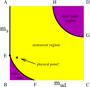
Figure 1.1: The conjectured phase diagram of QCD on the hypothetical $m_{s}$–$m_{ud}$ plane (strange quark mass versus light –up and down– quark mass, from now on we use degenerate light quark masses). The middle region corresponds to analytic crossover. In the purple (lower left and upper right) regions one expects a first order phase transition. On the boundaries between the first order phase transition regions and the crossover region and along the AE line the transition is of second order.

As a second step we leave the $\mu=0$ axis and study phenomena at non-vanishing baryonic densities. As we will see this is quite difficult, any method is spoiled by the sign problem, which we will discuss in detail. In the last 25 years several results were obtained for $\mu=0$ (though they were not extrapolated to the continuum limit). Until quite recently there were no methods, which were able to give any information on the non-vanishing chemical potential part of the phase diagram. In 2001 a method was suggested, with which the first informations were obtained and several questions could be answered. Using this –and other– methods we determine the phase diagram for small values of the chemical potential, we locate the critical point of QCD and similarly to the $\mu=0$ case we calculate the equation of state (note, that these results are not yet in the continuum limit, they are obtained at relatively large lattice spacings; for the continuum extrapolated results larger computational resources are necessary than available today).

1.1 The phase diagram of QCD

Before we discuss the results let us summarize the qualitative picture of the QCD phase diagram. Figure 1.1 shows the conjectured phase diagram of QCD as a hypothetical function of the $m_{ud}$ light quark mass and $m_{s}$ strange quark mass. In nature these quark masses are fixed and they correspond to a single point on this phase diagram. The figure shows our expectations for the nature of the transition. QCD is a gauge theory, which has two limiting cases with additional symmetries. One of these limiting cases correspond to the infinitely heavy quark masses (point D of the diagram). This is the pure SU(3) Yang-Mills theory, which has not only the SU(3) gauge symmetry but an additional Z(3) center symmetry, too. At high temperatures this Z(3) symmetry is spontaneously broken. The order parameter which belongs to the symmetry is the Polyakov loop. The physical phenomenon, which is related to the spontaneous symmetry breaking is the deconfining phase transition. At high temperatures the confining feature of the static potential disappears. The first lattice studies were carried out in the pure SU(2) gauge theory [1, 2]. The transition turned out to be a second order phase transition. Later on the increase of the computational resources allowed to study the SU(3) Yang-Mills theory. It was realized that in this case we are faced with a first order phase transition, which happens around 270 MeV in physical units [3, 4, 5, 6, 7].

The other important limiting case corresponds to vanishing quark masses (points A and B). In this case the Lagrangian has an additional global symmetry, namely chiral symmetry. Left and right handed quarks are transformed independently. Point A corresponds to a two flavour theory ($N_{f}=2$), whereas the three flavour theory ($N_{f}=3)$ is represented by point B. The chiral symmetry can be described by $U(N_{f})_{L}\times U(N_{f})_{R}$. At vanishing temperature the chiral symmetry is spontaneously broken, the corresponding Goldstone bosons are the pseudoscalar mesons (in the $N_{f}=2$ case we have three pions). Since in nature the quark masses are small but non-vanishing the chiral symmetry is only an approximative symmetry of the theory. Thus, the masses of the pions are small but non-zero (though they are much smaller than the masses of other hadrons). At high temperatures the chiral symmetry is restored. There is a phase transition between the low temperature chirally broken and the high temperature chirally symmetric phases. The corresponding order parameter is the chiral condensate. For this limiting case we do not have reliable lattice results (lattice simulations are prohibitively expensive for small quark masses, thus to reach the zero mass limit is extremely difficult). There are model studies, which start from the underlying symmetries of the theory. These studies predict a second order phase transition for the $N_{f}=2$ case, which belongs to the O(4) universality class. For the $N_{f}=3$ theory these studies predict a first order phase transition [8]. For intermediate quark masses we expect an analytic crossover (see Figure 1.1). One of the most important questions is to locate the physical point on this phase diagram, thus to determine the nature of the T>0 QCD transition for physical quark masses.

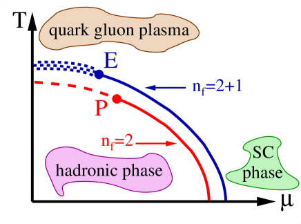
Figure 1.2: The most popular scenario for the $\mu$–$T$ phase diagram of QCD. For the massless $N_{f}=2$ case (red curve) we find a $P$ tricritical point between the second order (dashed line) and first order (solid lime) regions. For physical quark masses (two light quarks and another somewhat heavier strange quark: $N_{f}=2+1$, represented by the blue curves) the crossover (dotted region) and first order phase transition (solid line) regions are separated by a critical point $E$.

The most popular scenario for the $\mu$–$T$ phase diagram of QCD can be seen on Figure 1.2. At T=0 and at large chemical potentials model calculations predict a first order phase transition [9]. In two flavour massless QCD there is a tricritical point between the second order phase transition region (which starts at the second order point at $\mu=0$) and the first order phase transition region at large chemical potentials. As we will see QCD with physical quark messes is in the crossover region, thus in this case we expect a critical (end)point $E$ between the crossover and first order phase transition regions.

A particularly interesting picture is emerging at large chemical potentials. Due to asymptotic freedom at large densities we obtain a system with almost non-interactive fermions. Since quarks attract each other, it is easy to form Cooper-pairs, which results in a colour superconducting phase. The discussion of this interesting phenomenon is beyond the scope of the present summary.

The structure of the present work can be summarized as follows. In chapter 2 we summarize the necessary techniques of lattice gauge theory. Chapter 3 discusses the $\mu=0$ results. The nature of the transition is determined, its characteristic scale is calculated ($T_{c}$) and the equation of state is given. We discuss the $\mu\neq 0$ case in chapter 4. The source of the sign problem is presented and the multi-parameter reweighting is introduced. We determine the phase diagram, the critical point and the equation of state. Chapter 5 summarizes the results and provides a detailed outlook. Based on the available techniques and computer resources we estimate the time scales needed to reach the various milestones of lattice QCD thermodynamics.

2 QCD thermodynamics on the lattice

We summarize the most important ingredients of lattice QCD. Instead of providing a complete introduction we focus on those elements of the theory and techniques, which are essential to lattice thermodynamics. A detailed introduction to other fields of lattice QCD can be found in Ref. [10].

Thermodynamic observables are derived from the grand canonical partition function. The Euclidean partition function can be given by the following functional integral:

$$Z=\int{\cal D}U{\cal D}\bar{\psi}{\cal D}\psi e^{-S_{E}(U,\bar{\psi},\psi)},$$ (2.1)

here $U$ represent the gauge fields (gluons), whereas $\psi$ and $\bar{\psi}$ are the fermionic fields (quarks). QCD is an SU(3) gauge theory with fermions in the fundamental representation. Thus, at various space-time points the four components of the $U$ gauge field can be given by SU(3) matrices for all four directions. The fermions are represented by non-commuting Grassmann variables.

The Boltzmann factor is given by the Euclidean action, which is a functional of the gauge and fermionic fields. Equation (2.1) contains additional parameters (though they are not shown in the formula explicitely). These parameters are the $\beta$ gauge coupling (it is related to the continuum gauge coupling as $\beta=6/g^{2}$), the quark masses ($m_{i}$) and the chemical potentials ($\mu_{i}$). For simplicity equation (2.1) describes only one flavour. More than one flavour can be described by introducing several $\psi_{i}$ fields. In nature there are six quark flavours. The three heaviest flavours ($c,b,t$) are much heavier than the typical energy scales in our problem. They do not appear as initial or final states and they can not be produced at the typical energy scales. Their effects can be included by a simple redefinition of the other bare parameters (for some quantities they should be included explicitly as dynamical degrees of freedom, however, we will not discuss such processes). The three other quarks are the $u,d$ and $s$ quarks. The masses of the $u,d$ quarks are much smaller than the typical hadronic scale, therefore one can treat them as degenerate degrees of freedom (exact SU(2) symmetry is assumed). This approximation is satisfactory, since the mass difference between the $u$ and $d$ quarks can explain only $\approx$50% of the mass difference between different pions. For the remaining $\approx$50% the electromagnetic interaction is responsible (the up and down quarks have different electric charges). Including the mass differences would mean that one should include an equally important feature of nature, namely the electromagnetic interactions, too. This is usually far beyond the precision lattice calculations can reach today. Assuming $m_{u}=m_{d}$ is a very good approximation, the obtained results are quite precise, uncertainty related to this choice is clearly subdominant. For the degenerate up and down quark mass we use the shorthand notation $m_{ud}$. The $s$ quark is somewhat heavier, its mass is around the scale of the $\Lambda$ parameter of QCD. In typical lattice applications one uses the $m_{u}=m_{d}<m_{s}$ setup, which is usually called as $N_{f}=2+1$ flavour QCD.

In order to give the integration measure (${\cal D}U{\cal D}\bar{\psi}{\cal D}\psi$) one has to regularize the theory. Instead of using the continuum formulation we introduce a hypercubic space-time lattice $\Lambda$. The fields are defined on the sites (fermions) and on the links (gauge fields) of this lattice. It is easy to show that this choice automatically respects gauge invariance. For a given site $x\in\Lambda$ four $(x;\mu)$ links can be defined (here $\mu$ denotes the direction of the link, $\mu=1\dots 4$). Using this choice the integration measure is given by

$${\cal D}U{\cal D}\bar{\psi}{\cal D}\psi=\prod_{x\in\Lambda,\mu=1\dots 4}dU_{x;\mu}\prod_{x\in\Lambda}d\psi_{x}\prod_{x\in\Lambda}d\bar{\psi}_{x}$$ (2.2)

With this regularization one can imagine the functional integral as a sum of the Boltzmann factors $\exp(-E/kT)$ over all possible $\left\{U,\psi,\bar{\psi}\right\}$ configurations (here we use the $k=1$ convention). Thus, our system corresponds to a four-dimensional classical statistical system. The energy functional is simply replaced by the Euclidean action. An important difference is that in statistical physics the temperature is included in the Boltzmann factor, whereas in our case it is related to the temporal extent of the lattice (it is the inverse of it). It is easy to show that using periodic boundary conditions for the bosonic fields and antiperiodic boundary conditions for the fermionic fields our equation (2.1) reproduces the statistical physics partition function.

2.1 The action in lattice QCD

The lattice regularization means that one should discretize the Euclidean action $S_{E}$. This step is not unambiguous. There are several lattice actions, which all lead to the same continuum action. The difference between them is important, since these differences tell us how fast they approach the continuum result as we decrease the lattice spacing. Calculating a given $A$ observable on the lattice of a lattice spacing $a$, the result differs from the continuum one

$$\left<A\right>_{a}=\left<A\right>+{\cal O}(a^{\eta}).$$ (2.3)

The power $\eta$ depends on the way we discretized the action. The larger the power $\eta$ the better the action (for large $\eta$ we can obtain a result, which is quite close to the continuum one, already at large lattice spacing).

The most straightforward discretization is obtained by simply taking differences at neighbouring sites to approximate derivatives. Actions, which have better scaling behaviour (larger $\eta$ or smaller prefactor) are called improved actions.

In the following paragraphs we summarize the most important actions.

The action $S_{E}$ usually can be written as a sum $S_{E}=S_{g}+S_{f}$, where $S_{g}$ is the gauge action (it depends only on the gauge fields) and $S_{f}$ is the fermionic action (it depends both on the gauge and fermionic fields).

The simplest gauge action is the Wilson gauge action which is the sum of the

$$U_{P}(x;\mu\nu)=U_{x;\mu}U_{x+a\hat{\mu};\nu}U^{\dagger}_{x+a\hat{\nu};\mu}U^{\dagger}_{x;\nu}$$ (2.4)

plaquettes. Here $\hat{\mu}$ denotes the unit vector in the $\mu$ direction. The Wilson action reads:

$$S_{g,\rm{Wilson}}=-\beta\left(\frac{1}{3}\sum_{x,\mu<\nu}{\rm Re}{\rm Tr}U_{P}(x;\mu\nu)-1\right)$$ (2.5)

This action is the simplest real, gauge invariant expression, which can be constructed using the gauge fields. One can show, that in the continuum limit the above expression leads to the usual Yang-Mills gauge action.

One can improve the action by adding other gauge invariant terms. The simplest such improvement term is provided by the $2\times 1$ rectangles, for which –analogously to the plaquette term– we multiply the SU(3) link matrices around the rectangle. Denoting this term by $U_{2\times 1}(x;\mu\nu)$ one obtains the following action

$$S_{g}=-\frac{\beta}{3}\left(c_{0}\sum_{x,\mu<\nu}{\rm Re}{\rm Tr}U_{P}(x;\mu\nu)+c_{1}\sum_{x,\mu\neq\nu}{\rm Re}{\rm Tr}U_{2\times 1}(x;\mu\nu)\right)$$ (2.6)

It can be shown that this choice improves the scaling. On the tree level the condition $c_{0}+8c_{1}=1$ should be fulfilled and $c_{1}=-1/12$. This is the (tree level improved) Symanzik gauge action. Other improvements use also chair-like closed paths and non-perturbative coefficients. Note, however that the tree level improvement is usually enough for thermodynamic studies, the main source of difficulties is in the fermionic part (further improvements in the gauge sector can be considered as a sort of “over-killing”).

Discretizing the fermionic fields is more difficult than discretizing gauge fields. The naive discretization leads to the following action

$$S_{f,\mbox{\small naive}}=\sum_{x}\left[am\bar{\psi}\psi+\frac{1}{2}\sum_{\mu=1\dots 4}\left(\bar{\psi}_{x}U_{x;\mu}\gamma_{\mu}\psi_{x+a\hat{\mu}}-\bar{\psi}_{x}U^{\dagger}_{x-a\hat{\mu};\mu}\gamma_{\mu}\psi_{x-a\hat{\mu}}\right)\right].$$ (2.7)

in the free case ($U=1$) the propagator has 16 poles in the Brillouin zone (we expected only one). Thus, contrary to the continuum case our lattice action describes 16 degenerate fermions instead of 1 fermion.

There are several ways to resolve this problem. The two most popular solutions are the Wilson and the Kogut-Susskind regularizations. The problem is related to the fact that the continuum fermion action contains only first derivatives. The basic idea of the Wilson fix is to add a second derivative term –Wilson term– to the action: $a\bar{\psi}\partial_{\mu}\partial_{\mu}\psi$. This term vanishes in the continuum limit. For non-vanishing lattice spacings the Wilson term increases the masses of the 15 non-physical modes so that they are at the cutoff scale ($1/a$). As we approach the continuum limit these 15 particles decouple. Generally, one can use a Wilson term with an arbitrary coefficient $r$. The usual choice is $r=1$. In this case the action reads

$$S_{f,\rm{Wilson}}=\sum_{x}\left[\bar{\psi}\psi+\kappa\sum_{\mu=1\dots 4}\left(\bar{\psi}_{x}U_{x;\mu}(1+\gamma_{\mu})\psi_{x+a\hat{\mu}}+\bar{\psi}_{x}U^{\dagger}_{x-a\hat{\mu};\mu}(1-\gamma_{\mu})\psi_{x-a\hat{\mu}}\right)\right].$$ (2.8)

Here the fields are rescaled appropriately. The disadvantage of Wilson fermions is the loss of chiral symmetry for vanishing quark masses. This symmetry is restored only in the continuum limit. The quark mass receives an additive renormalization and the asymptotic scaling (c.f. equation (2.3)) is linear in $a$.

Kogut and Susskind introduced another formalism, namely the staggered fermions. The spinor components of the fermionic field are distributed among the corners of a $2^{4}$ hypercube. This leads to a diagonal expression in the spinor index. By using only 1 out these 4 diagonal components one can reduce the number of degrees of freedom by a factor of 4. This action describes 16/4=4 fermions of the same mass. The action can be written as

$$S_{f,\rm{staggered}}=\sum_{x}\left[am\bar{\chi}\chi+\frac{1}{2}\sum_{\mu=1\dots 4}\alpha_{x;\mu}\left(\bar{\chi}_{x}U_{x;\mu}\chi_{x+a\hat{\mu}}-\bar{\chi}_{x}U^{\dagger}_{x-a\hat{\mu};\mu}\chi_{x-a\hat{\mu}}\right)\right],$$ (2.9)

where $\alpha_{x;\mu}=(-1)^{x_{1}+\dots+x_{\mu-1}}$. Contrary to the naive or Wilson fermion formulations the $\chi$ field has only one spin component. For simplicity we use the Greek letter $\psi$ also for staggered fermions. The most important advantage of the staggered formalism is, that the action has a $U(1)_{L}\times U(1)_{R}$ symmetry (which is a remnant of the original chiral symmetry). Due to this symmetry there is no additive mass renormalization. The asymptotic scaling is better than for Wilson fermions, it is proportional to $a^{2}$. An additional advantage is of computational nature. Since we do not have Dirac indices the computations are faster. The most important disadvantage of the staggered fermions is the fourfold degeneracy of the fermions. Later we discuss the technique, which allows one to use less than four fermions.

In principle, there are several other fermion formulations. Note, however, that the Nielsen-Ninomiya no-go theorem excludes any continuum-like fermion formulations [11, 12]. According to this theorem one can not have a local fermion formulation with a proper continuum limit for one flavour, which respects chiral symmetry. Recently, it was possible to construct a fermion formulation, which fulfills the above conditions and respects a modified (lattice-like) chiral symmetry [13, 14]. These fermions are called chiral lattice fermions. They represent a mathematically elegant formulation with many important features, which make lattice calculations unambiguous and straightforward. Unfortunately, they are extremely CPU demanding, they require approximately two orders of magnitude more computer time than the more traditional Wilson or staggered fermions. The first steps in order to develop reliable algorithms have been made and exploratory studies have been carried out on relatively small lattices [15, 16, 17, 18, 19, 20]. We expect that in the near future important results will be obtained by using chiral lattice fermions.

Both eq. (2.8) and (2.9) are bilinear in the fermionic fields (it is true for other actions, too):

$$S_{f}=\sum_{x,y}\bar{\psi}_{x}M_{xy}(U)\psi_{y},$$ (2.10)

here the specific form of the matrix $M$ can be derived from eq. (2.8) and (2.9). Since the fermionic fields are represented by Grassmann variables it is difficult to treat them numerically. We do not know any technique, which can be used as effectively as the bosonic importance sampling methods. Fortunately, the fermionic integrals can be evaluated exactly. Using the known Grassmann integration rules one obtains:

$$\int{\cal D}\bar{\psi}{\cal D}\psi e^{-S_{f}}=\det M(U),$$ (2.11)

Thus the partition function (2.1) can be written as follows:

$$Z=\int{\cal D}U\det M(U)e^{-S_{g}(U)}=\int{\cal D}Ue^{-\left\{S_{g}(U)-\ln\det M\right\}}.$$ (2.12)

This simple step resulted in an effective theory, which contains only bosonic fields. The action reads: $S_{\rm{eff.}}=S_{g}-\ln\det M$. Unfortunately this action is non-local. Due to the fermionic determinant fields at arbitrary distances interact with each other (the original action $S_{E}=S_{g}+S_{f}$ is local in the field variables). This non-locality is the most important source of difficulties. It is much more demanding to study full QCD (with dynamical fermions) than pure SU(3) gauge theory.

For the 2+1 flavour theory we need different fermionic fields. Each fermionic integration results in a fermionic determinant. These determinants depend explicitely on the quark masses:

$$Z(m_{1},m_{2},\dots m_{N_{f}})=\int{\cal D}U\det M(m_{1};U)\det M(m_{2};U)\dots\det M(m_{N_{f}};U)e^{-S_{g}(U)}.$$ (2.13)

For Wilson fermions the above formula can be used directly for 2+1 flavours. For staggered fermions another trick is needed. Since one $\psi$ field describes four fermions in the staggered formalism one uses the fourth root trick. The reason for that is quite simple. For more than one field one uses powers of the determinant. Analogously for one flavour one uses the fourth root of the determinant. We expect that the partition function

$$Z(N_{f})=\int{\cal D}U\left[\det M(U)\right]^{N_{f}/4}e^{-S_{g}(U)}$$ (2.14)

describes $N_{f}$ flavours in the staggered theory. Note, however, that the locality of such a model is not obvious. As we saw the partition function 2.12) was the result of a local theory, which is not necessarily the case for (2.14). This question is still debated in the literature (see e.g.  [21]). Though the theoretical picture is not clear, all numerical results show that the fourth root trick most probably leads to a proper description of one flavour of QCD.

In the rest of this work we will deal with staggered theory, only. Since staggered fermions are computationally less demanding than other fermion formulations, the vast majority of the results in the literature are obtained by using staggered fermions. Another reason why the staggered fermions are so popular for thermodynamic studies is related to the fact that staggered fermions are invariant under (reduced) chiral symmetry, which might play an important role for questions such as chiral symmetry restoration (at the finite temperature QCD transition).

In numerical simulations we use finite size lattices of $N_{s}^{3}N_{t}$. The three spatial sizes are usually the same ($N_{s}$), they give the spacial volume of the system, whereas the temporal extension in Euclidean space-time is directly related to the temperature:

$$V=(N_{s}a)^{3}, T=\frac{1}{N_{t}a}.$$ (2.15)

Lattices with $N_{t}\geq N_{s}$ are called “zero temperature” lattices, and lattices with $N_{t}\ll N_{s}$ are called “non-zero temperature” lattices. In thermodynamic studies a small temperature region around the transition temperature is the main focus of the analyses (an exception is the determination of the equation of state, which can be studied at much higher temperatures, too). According to $T=1/(N_{t}a)$ one can fix the temperature by using smaller and smaller lattice spacings and larger and larger $N_{t}$ temporal extensions. Thus, the resolution of an analysis is usually characterized by the temporal extension. In the literature one finds typically $N_{t}$ values of 4, 6, 8 and 10, which correspond to lattice spacings (at and around $T_{c}$) of approximately $a=$0.3, 0.2, 0.15 and 0.12 fm, respectively. We give here only approximative values and it is impossible to give precise values for the lattice spacings, particularly for these relatively coarse lattices. The reason for this “no-go” observation can be summarized as follows. QCD predicts only dimensionless combinations of observables. These combinations are only approximated on the lattices, they have $a^{\eta}$ scaling corrections, which vanish as we approach the continuum limit. Since different combinations have different scaling corrections, the lattice spacing can not be given unambiguously.

The lattice spacing defines a cutoff $\Lambda\sim 1/a$. One of the most important source of difficulties is related to the fact that we want to ensure that all masses we study are smaller than the cutoff, whereas all Compton wave-lengths (which are proportional to the inverse masses) are much smaller than the size of the lattice (otherwise one has large finite volume effects). Since in QCD we have masses, which are quite different (the mass ratio of the nucleon and pion is about seven) we are faced with a multi-scale problem. This results in a quite severe lower bound on $N_{t}$. In earlier works the only way to deal with such a multi-scale problem was to ignore that in nature we have such a phenomenon. People used a much smaller nucleon to pion mass ratio than the physical one, thus they used quite heavy quark masses, which resulted in heavy pion masses. Since the transition is related to the chiral features of the theory (we speak about chiral transition) this approximation is clearly non-physical. Another reason to use larger than physical pion masses is of algorithmic nature.

2.2 Correlators

The expectation value of an observable $O$ can be given as a functional integral over the $U$ and $\psi_{i},\bar{\psi}_{i}$ fields:

$$\left<O\right>=\frac{1}{Z}\int{\cal D}U{\cal D}\bar{\psi}{\cal D}\psi O\left[U,\bar{\psi},\psi\right]e^{-S_{E}(U,\bar{\psi},\psi)}.$$ (2.16)

Quantum field theories can be defined by operators. Formally, defining the theory by $\hat{O}$ operators or defining it by the above functional integral are identical. The results in the two formalisms are the same $\langle\hat{O}\rangle=\langle O\rangle$.

At zero temperature typical choices of operators are n-point functions of the fields. Particularly important n-point functions are the two-point functions (propagators). E.g. for pions the interpolating operator $\hat{O}$ can be given as $\hat{O}=\hat{\bar{\psi}}_{u}\gamma_{5}\hat{\psi}_{d}$. The u,d indices denote up and down quarks. The (Euclidean) time evolution of the $\hat{O}$ operator is given by the Hamiltonian $\hat{H}$ by the usual way: $\hat{O}(t)=e^{t\hat{H}}\hat{O}(0)e^{-t\hat{H}}$. Thus, inserting a complete set of energy eigenstates $\left|n\right>$, the two-point function can be written as

$$\left<0\right|\hat{O}(t)\hat{\bar{O}}(0)\left|0\right>=\sum_{n}\left|\left<0\right|\hat{O}\left|n\right>\right|^{2}e^{-(E_{n}-E_{0})t}.$$ (2.17)

For large $t$ values the above function is dominated by the term with the smallest $E_{n}$ (assuming that its prefactor is non-vanishing). Thus, for a given chanel the exponential decay of the two-point function of the operator $\hat{O}$ (with the proper quantum numbers) provides us with the smallest energy (mass). The correlation length $\xi$ is proportional to the inverse of the mass. In lattice units $\xi=1/(ma)$, where $\xi$ denotes this dimensionless correlation length (in lattice units). Using the appropriate operators one can determine the masses of hadrons on the lattice.

2.3 Continuum limit

The final goal of lattice QCD is to give physical answers in the continuum limit. Results at various lattice spacings ‘$a$’ are considered as intermediate steps. Since the regularization (lattice) is inherently related to the non-vanishing lattice spacing it is not possible to carry out calculations already in the continuum limit in our lattice framework. The continuum physics appears as a limiting result. Obviously, the $a\rightarrow 0$ limit should be carried out according to eq. (2.3). During this procedure the physical observables, more precisely their dimensionless combinations should converge to finite values. On the way to the continuum limit one should tune the parameters of the Lagrangian as a function of the lattice spacing. The renormalization group equations tell us how the parameters of the Lagrangian depend on the lattice spacing. For small gauge coupling (thus, for large cutoff or close to the continuum limit) the perturbative form of the renormalization group equations can be used. For somewhat larger gauge couplings one should use non-perturbative relationships.

As we have seen, the correlation length $\xi$ of a hadronic interpolating operator is proportional to the inverse mass of the hadron $\xi=1/(ma)$. In order to reach the continuum limit the lattice spacing in physical unit should approach zero: $a\rightarrow 0$. Since the hadron mass is a finite value in the same physical units, the correlation length $\xi$ should diverge. Thus the continuum limit of lattice QCD is analogous to the critical point of a statistical physics system (which is also characterized by a diverging correlation length). The Kadanoff-Wilson renormalization group of statistical physics can be used for lattice QCD, too. The renormalization group transformation tells us how to change the parameters of the lattice action (Lagrangian) in order to obtain the same large distance behaviour (the small distance behaviour is not important for us, it merely reflects our discretization process). This was the original idea of Wilson: one has to carry out a few renormalization group transformation with increasing ‘$a$’ and describe QCD by an action which is “good enough” at these large lattice spacings. After these steps the action can be used for a numerical solution. Unfortunately, the renormalization group transformation procedure results in an action, which is far too complicated to be used . Usually, when one changes the lattice spacing (e.g. all the way to the continuum limit) the form of the action remains the same, only its parameters are changed. The way the parameters change is called renormalization group flow or line of constant physics (LCP). It can be obtained by choosing a few dimensionless combinations of observables and demanding that their values remain the same “predefined” value as we change the lattice spacing. Using different sets of observables result in different LCPs; however, these different LCPs merge when we approach the continuum limit. The LCPs are usually determined by non-perturbative techniques. The simplest procedure is to measure the necessary dimensionless combinations at various parameters of the action (bare parameters) and interpolate to those bare parameters, at which the dimensionless combinations take their predefined value. A few iterative steps are usually enough to reach the necessary accuracy.

2.4 Algorithms

The determination of expectation values of various observables is the most important goal of lattice gauge theory. To that end one has to evaluate multi-dimensional integrals. Since the dimension can be as high as $10^{9}$, which is the state of the art these days, it is a non-trivial numerical work. The systematic mapping of such a multi-dimensional function is clearly impractical. The only known method to handle the problem is based on Monte-Carlo techniques. We chose some configurations randomly and calculate the observables on these fields. The seemingly simplest method is to generate configurations with a uniform distribution (uniform in the integration measure). This choice is quite inefficient, since the Boltzmann factor exponentially suppresses most of these terms. Only a few configurations would give a sizable contribution, and using a uniform distribution the probability of finding these configurations is extremely small. The most efficient technique, which is available today, is based on importance sampling. The configurations are not uniformly generated, instead one uses a distribution $p\propto e^{-S_{E}}$ for the generation. Thus, those configurations, which contribute with a large Boltzmann weight are chosen more probably ($e^{-S_{E}}$ is large) than those, which contribute with a small Boltzmann factor ($e^{-S_{E}}$ is small). For the case of QCD the Euclidean action $S_{E}$ contains the bosonic and the fermionic fields, which are represented by Grassmann variables. There is no known importance sampling based procedure for Grassmann variables. As we discussed already one has to evaluate the fermionic integral explicitely. This integration leads to (2.12). Thus, a procedure based on importance sampling uses the distribution $p(U)\propto\det M(U)e^{-S_{g}(U)}$ for generating the configurations. Let us assume that we have an infinitely large ensemble of configurations, given by the above distribution. The expectation value of an observable $O$ can be calculated as

$$\left<O\right>=\lim_{N\to\infty}\frac{1}{N}\sum_{i=1}^{N}O(U_{i}).$$ (2.18)

In practice our ensemble is always finite, thus the $N\to\infty$ limit can not be achieved, $N$ remains finite. The lack of this infinite limit results in statistical uncertainties. One standard technique to determine the statistical errors is the jackknife method [10].

A crucial ingredient of any method based on importance sampling is the positivity of $\det M(U)$ (it should be a positive real number) for all possible $U$ gauge configurations. Otherwise the expression $\det M(U)e^{-S_{g}(U)}$ can not be interpreted as a probability. In order to illustrate the importance of this condition we shortly summarize the simplest importance sampling based Monte-Carlo method, the Metropolis algorithm. All known techniques represent a Markov chain, in which the individual configurations of the ensemble are obtained from the previous configurations. The Metropolis algorithm consists of two steps. In the first step we change the configuration $U$ randomly and obtain a new configuration $U^{\prime}$. Obviously, this configuration has a different Boltzmann factor. In the second step we take account for this difference and accept this new $U^{\prime}$ configuration, as a member of our ensemble, with the probability

$$P(U^{\prime}\leftarrow U)=\min\left[1,e^{-\Delta S_{g}}\frac{\det M(U^{\prime})}{\det M(U)}\right],$$ (2.19)

where $\Delta S_{g}=S_{g}(U^{\prime})-S_{g}(U)$. If the configuration $U^{\prime}$ was not accepted (the probability of this case is $1-P(U^{\prime}\leftarrow U)$), we keep the original configuration $U$. It can be easily seen that $0\leq P(U^{\prime}\leftarrow U)\leq 1$ is fulfilled only if $\det M$ is positive and real.

Interestingly, this non-trivial condition is fulfilled, it is a consequence of the $\gamma_{5}$ hermiticity of the $M$ fermion matrix (or in other words Dirac operator)

$$M^{\dagger}=\gamma_{5}M\gamma_{5}.$$ (2.20)

This equality can be easily checked both in the continuum formulation (2.8) or for the lattice formulations (2.9).

If $v$ is an eigenvector of $M^{\dagger}$ with eigenvalue $\lambda$ then $\lambda v=M^{\dagger}v=\gamma_{5}M\gamma_{5}v$. This gives $\lambda\gamma_{5}v=M\gamma_{5}v$. Thus, $\lambda$ is an eigenvalue of $M$. It can be similarly shown that an eigenvalue of $M$ is also an eigenvalue of $M^{\dagger}$. Thus, $M$ and $M^{\dagger}$ have the same eigenvalues. As a result, these eigenvalues are either real or appear in conjugate pairs. As a consequence $\det M$ is always real. In the continuum theory and for staggered fermions the massless Dirac operator has only purely imaginary eigenvalues, thus the real eigenvalues of the massive Dirac operator are always positive (they are equal to the quark mass). In these cases the condition $\det M\geq 0$ is fulfilled and the equality appears only for vanishing quark masses. For Wilson fermions negative eigenvalues might appear. Note; however, that these eigenvalues disappear as we approach the continuum limit. For Wilson fermions the most straightforward method is to use two degenerate quarks, thus $(\det M)^{2}$ can be used. Alternatively one can take one flavour with $\left|\det M\right|$. Since in the continuum limit $\det M$ is a positive real number, taking the absolute value does not influence the continuum limit.

It is important to note already at this stage that for non-vanishing baryonic chemical potentials the $\gamma_{5}$ hermiticity of the Dirac operator is not fulfilled, thus the determinant is not necessarily a real positive number. The partition function itself will be always real, thus one can use the real part of the integrand. Note, however, that the real part of the determinant can be positive or negative. In the sum large cancellations appear between the terms with different signs. This is the sign problem, which makes studies at non-vanishing chemical potential extremely difficult. As a consequence importance sampling such as the Metropolis algorithm does not work.

The Metropolis algorithm generates the configurations according to the proper distribution. Unfortunately, it is a quite inefficient algorithm. There are two reasons for that. First of all, one has to calculate the determinant of the Dirac operator in each step, which is quite CPU demanding, it scales with the third power of $N_{s}^{3}N_{t}$. Secondly, the subsequently generated configurations in the Markov chain are not independent of each other (for rejected configurations they are even identical). As it turns out the autocorrelation is huge.

There are several algorithms on the market, which are much more efficient. The most widely used method is the so-called Hybrid Monte-Carlo (HMC) algorithm [24, 25, 26]. We shortly summarize the basic ideas to this technique. The determinant of any positive definite, hermitian $H$ can be written as a functional integral over bosonic fields

$$\det H=\frac{\int{\cal D}\Phi^{\dagger}{\cal D}\Phi e^{-\Phi^{\dagger}H^{-1}\Phi}}{\int{\cal D}\Phi^{\dagger}{\cal D}\Phi e^{-\Phi^{\dagger}\Phi}}.$$ (2.21)

(On a finite lattice the integral is a large –but finite– dimensional integral.)

Since the fermion matrix $M$ is usually not hermitian we usually use $H=M^{\dagger}M$. This choice describes two fermions/flavours in the continuum or in the Wilson formalism (or 8 fermions in the staggered formalism, for staggered fermions one uses the word taste instead of flavour). In order to describe $N_{f}$ fermion flavors (tastes) $H=(M^{\dagger}M)^{N_{f}/2}$ is used (in the staggered case $H=(M^{\dagger}M)^{N_{f}/8}$ is the proper choice). Note, that these steps result in several problems, which we will discuss later.

The partition function for two degenerate quarks reeds

$$Z=C\int{\cal D}U{\cal D}\Phi^{\dagger}{\cal D}\Phi e^{-S_{g}(U)-\Phi^{\dagger}\left(M^{\dagger}M\right)^{-1}\Phi},$$ (2.22)

where the denominator of (2.21), which gives only an irrelevant prefactor to $Z$, is denoted by $1/C$. Let us assign to each lattice link a traceless anti-hermitian matrix $\Pi_{x\mu}$, for which $\Pi^{2}/2=\sum_{x;\mu}\left|\Pi_{x\mu}\right|^{2}/2$. Multiplying $Z$ by the constant $1/C^{\prime}=\int{\cal D}\Pi\exp\left(-\Pi^{2}/2\right)$ we obtain

$$Z=C^{\prime}C\int{\cal D}\Pi{\cal D}U{\cal D}\Phi^{\dagger}{\cal D}\Phi e^{-\Pi^{2}/2-S_{g}(U)-\Phi^{\dagger}\left(M^{\dagger}M\right)^{-1}\Phi}.$$ (2.23)

For fixed $\Phi^{\dagger},\Phi$ one can define a function

$${\cal H}(U,\Pi)=\Pi^{2}/2+S_{g}(U)+\Phi^{\dagger}\left(M(U)^{\dagger}M(U)\right)^{-1}\Phi,$$ (2.24)

which depends on the $U_{x\mu}$ and $\Pi_{x\mu}$ matrices (here $x\mu$ parameterizes the links). We can consider $H$ as the Hamiltonian of a classical many-particle system with general coordinates of $U_{x\mu}$ and general momenta of $\Pi_{x\mu}$. It is possible to solve the canonical equations of motions in a fictious time $t$. Along such trajectories the Hamiltonian ${\cal H}$ is constant. Thus, for the $U$ and $P$ fields we can introduce a Metropolis step (thus a new $U^{\prime}$ and $P^{\prime}$) for which the integrand of (2.23) does not change and the acceptance probability is 1. The update of the $\Phi^{\dagger},\Phi$ fields is done by a global heatbath. The calculation of the trajectories are done numerically, thus the Hamiltonian is not conserved exactly. It can be shown that for the leapfrog integration (which is the most common choice in the literature) the change in the Hamiltonian is proportional to the integration step-size squared: $\Delta{\cal H}\propto\varepsilon^{2}$. In order to have an exact algorithm one has to carry out at the end of each trajectory an additional Metropolis accept/reject step. This concludes the necessary steps of a Hybrid Monte-Carlo algorithm, which we summarize here.

1. For a fixed gauge field $U$ we generate $\Pi$, $\Phi^{\dagger}$ and $\Phi$ configurations. The generation is done via a global heatbath according to the integrand.

2. The canonical equation of motions are integrated numerically from $t=0$ to $T$ using a step-size of $\varepsilon$. The usual choice is $T=1$.

3. The configuration $U^{\prime}$ at the end of the trajectory is accepted with probability of

   $$P(U^{\prime}\leftarrow U)=\min\left[1,e^{-\Delta{\cal H}}\right].$$ (2.25)

   $\Pi^{\prime}$, $\Phi^{\dagger}$ and $\Phi$ are not needed any more, for the next trajectory they will be regenerated as discussed in our first step.

It can be proven, that repeating this procedure gives the proper distribution for the gauge configurations. The most demanding calculation numerically is the integration of the second step and the calculation of the term $\left(M^{\dagger}M\right)^{-1}\Phi$ in the third step. An identical question is to solve the linear equation of

$$\Phi=\left(M^{\dagger}M\right)\chi.$$ (2.26)

The standard procedure is the conjugate gradient method. Since the matrix is sparse this method gives the solution, of the necessary precision, in $c\cdot L_{s}^{3}L_{t}$ steps. The coefficient $c$ is proportional to the condition number of the $M$ matrix. The smallest eigenvalue of the matrix $M$ is the quark mass (for the Wilson formalism, even smaller eigenvalues can appear). The largest eigenvalue is a quark mass independent constant. Thus, the time needed for the computation is inversely proportional to the quark mass. This is the reason for the increase of the CPU costs for small quark masses, which makes calculations in lattice QCD with physical quark masses quite challenging.

As we discussed, for one flavour or taste fractional powers of the expression $\left(M^{\dagger}M\right)$ should be taken. In this case the standard conjugate gradient method can not be applied: $\left(M^{\dagger}M\right)^{-N_{f}/2}\Phi$ (for the staggered formalism the power $-N_{f}/8$ should be used). It can be shown that in the second step of the algorithm only integer powers of the fermion matrix is needed, and the inversions can be carried out. In the third step, however, the fractional power can not be avoided. Until recently no efficient method was known to treat fractional powers, the most widely used method, the $R$ algorithm [27] simply omitted the third step. For small enough $\varepsilon^{2}$ the change in the Hamiltonian was small, too: $\Delta{\cal H}\propto\varepsilon^{2}$. The method was not exact. In order to produce unambiguous results one had to carry out a $\varepsilon\to 0$ extrapolation, which was usually omitted.

Recently, a new method appeared in the literature, which solved this problem. In this rational Hybrid Monte-Carlo (RHMC) algorithm the fractional powers are approximated by rational functions. Using 10-15 orders one can [28] approximate the fractional powers upto machine precision. Using this technique all three steps of the Hybrid Monte-Carlo method can be done for arbitrary $N_{f}$ exactly. Interestingly enough, the exact rational Hybrid Monte-Carlo algorithm turned out to be faster than the non-exact $R$ algorithm.

3 Results at zero chemical potential

We start the review of recent results with the $\mu=0$ case. Results on the order of the transition, the absolute temperature of the transition and the equation of state will be discussed.

All thermodynamics studies are based on two main steps. The observables relevant for locating and describing the transition are determined on high temperature ($N_{s}\gg N_{t}$) lattices. Thus, $T>0$ simulations is one of the necessary ingredients.

In order to set the parameters of the action and to give temperatures in physical values (in MeV), some observables (as many of them as many parameters the action has) have to be compared to their experimental values. The parameters of the action have to be tuned so that these selected observables agree with their experimental values. Since sufficiently high precision experimental values, such as hadron masses, are currently only available at zero temperature, this step can only be completed via $T=0$ simulations. Since the parameters of the action, which are then used for the $T>0$ simulations, are set in this step, it is useful to start with the $T=0$ simulations and then proceed with the $T>0$ ones.

3.1 Choice of the action

In chapter 2 we have seen that the choice of the lattice action has a significant impact on the continuum extrapolation. On the one hand, an improved action can make it possible to do a reliable extrapolation from larger lattice spacings than with an unimproved action. On the other hand the computational needs of improved actions are often much higher than in the unimproved case. In the following we review the actions used by different collaborations in large scale lattice thermodynamics calculations.

In the gauge sector typically the (2.6) Symanzik improved action is used either with tree level coefficients or with tadpole improvement. This improves the scaling of the action significantly compared to the unimproved Wilson action at an acceptable cost.

In the fermionic sector upto now all large scale thermodynamics studies were carried out with staggered fermions. The main reasons why most collaborations take this choice is the computational efficiency and the remnant chiral symmetry of staggered fermions. The MILC collaboration uses ASQTAD fermions, the RBC-Bielefeld collaboration uses p4 improved fermions and the Wuppertal-Budapest group stout improved fermions. The two former are described in detail in Ref. [29] while the latter was originally introduced in [30] and the used parameters can be found in Ref. [31].

Free staggered fermions describe four degenerate quark flavors. In the interacting case, however, due to taste symmetry violation the quark masses and the corresponding pseudoscalar masses will only become degenerate in the continuum limit. This feature is also present in the 2+1 flavor theory obtained via the rooting trick. At the lattice spacings typically used for thermodynamics studies, the second lightest pseudoscalar mass can easily be three-four times heavier than the lightest one. Since the order of the transition depends on the number of quark flavors, it is desirable to use an action where taste symmetry violation is significantly reduced. Figure 3.1 shows the taste symmetry violation for the three actions discussed above. We can see that stout smearing is the most effective in reducing taste symmetry violation.

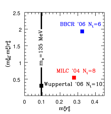
Figure 3.1: Taste symmetry violation of three different lattice actions: ASQTAD improved action used by the MILC collaboration [32], p4 action used by the RBC-Bielefeld collaboration [33] and the stout improved action used by the Wuppertal-Budapest group [34]. The taste symmetry violation is characterized by the difference of the squares of the two lightest pions. All quantities are normalized by the $r_{0}$ Sommer scale. The vertical line indicates the physical pion mass.

3.2 T=0 simulations

3.2.1 Determination of the LCP

In lattice calculations of QCD thermodynamics we usually determine some observables at several different temperatures. Since the temperature is inversely proportional to the temporal extent of the lattice: $T=1/(N_{t}a)$, there are two ways to change the temperature. One can either change $N_{t}$ or the lattice spacing. Since $N_{t}$ is an integer, the first possibility gives reach only for a discrete set of temperatures. Therefore the temperature is usually tuned by changing the lattice spacing at fixed $N_{t}$. This means that, as discussed in chapter 2, while changing the lattice spacing we have to properly tune the parameters of the action to stay on the Line of Constant Physics (LCP).

Since the action has three parameters ($\beta$ and the quark masses), we have to choose three physical quantities. Usually one of these quantities is used to set the physical scale while two independent dimensionless ratios of the three quantities defines the LCP. We have to choose such quantities whose experimental values are well known. Since according to chiral perturbation theory the pseudoscalar meson masses ($m_{PS}$) are directly connected to quark masses ($m^{2}_{PS}\propto m_{q}$), they are good candidates to set the quark mass parameters. In case of 2+1 flavors this means the masses of pions ($m_{\pi}$) and kaons ($m_{K}$). For the third quantity there are several possibilities. It is useful to choose an observable which has a weak quark mass dependence.

Up to very recently the most common way to set the physical scale was via the static quark-antiquark potential. Both the MILC and RBC-Bielefeld collaborations are still using this technique. On the lattice the static potential can be determined with the help of Wilson-loops. A $W_{x;\mu}(R,T)$ Wilson-loop of size $R\times T$ is an observable similar to the plaquette where we take the product of the links along a rectangle of size $R\times T$. The first, spatial direction of the rectangle is characterized by $\mu=1\dots 3$, whereas the second direction is always the Euclidean time. One can define the Wilson-loop average as:

$$W(R,T)={\rm Re}{\rm Tr}\sum_{x;\mu=1\dots 3}W_{x;\mu}(R,T)$$ (3.1)

It can be shown that the free energy (at zero temperature the potential energy) of a system with an infinitely heavy quark-antiquark pair separated by a distance $R$ is given by

$$V(R)=-\lim_{T\to\infty}\frac{1}{T}\ln W(R,T).$$ (3.2)

There are two useful quantities which can be easily obtained from $V(R)$ and they are usually used for scale setting. The first one is the $\sigma$ string tension which is defined as $\sigma=\lim_{R\to\infty}dV(R)/dR$. While $\sigma$ is a useful quantity in the pure gauge theory –where the potential is linear for large $R$–, in QCD it does not exist in a strict sense. At large distances pair creation will lead to string breaking and the potential will saturate. Nevertheless, $\sigma$ is still sometimes used to set the scale in full QCD.

The second quantity obtained from $V(R)$ is the Sommer parameter, $r_{0}$, which is defined implicitly by [35]:

$$\left.R^{2}\frac{dV(R)}{dR}\right|_{R=r_{0}}=1.65.$$ (3.3)

Both quantities have the great disadvantage that they can not be measured directly by experiments. Their values can only be estimated from e.g. heavy meson spectroscopy. The value of the string tension is $\sqrt{\sigma}\approx$440 MeV, while for $r_{0}$ the most accurate values are based on lattice calculations (where the scale was set with some other quantity of course) [36, 37]: $r_{0}=$0.469(7) fm, other values are 0.444(3) (based on the pion decay constant[38], 0.467(33) from QCDSF [39] and 0.492(6)(7) from PACS-CS [40]. Note, that there are several sigma differences between these results. This fact emphasizes the general observation, that the determination of $r_{0}$ is difficult, and that the systematic errors are underestimated.

It may be desirable to use a quantity which is well known experimentally. The nucleon mass may seem as an obvious choice, however, on the lattice spacings typical in thermodynamics studies, an accurate lattice determination of the nucleon mass is difficult. Another choice, which is often used in the literature, is the $\rho$ meson mass. Unfortunately as it is a resonance, its precise mass determination would require a detailed analysis of its interaction with the decay products.

The quantity used by the Wuppertal-Budapest group is the leptonic decay constant of the kaon: $f_{K}=159.8$ MeV, whose experimental value is known to about one percent accuracy and it can be precisely determined on the lattice . Let us now illustrate the determination of the LCP and the scale setting with the $m_{\pi},m_{K},f_{K}$ choice.

For any set of the dimensionless bare parameters ( $\beta$, $am_{ud}$ and $am_{s}$) we can determine $am_{\pi}$, $am_{K}$ and $af_{K}$ on the lattice. For a fixed $\beta$ we can set $am_{ud}$ and $am_{s}$ such that the ratios $(am_{\pi})/(af_{K})$ and $(am_{K})/(af_{K})$ agree with the physical $m_{\pi}/f_{K}$ and $m_{K}/f_{K}$ ratios. This way we have an $am_{ud}(\beta)$ and an $am_{s}(\beta)$ function. We call these functions LCP. The lattice spacing is given by the third quantity: $a=(af_{K})/(159.8\rm{MeV})$. Figure 3.2 shows the LCP obtained this way using stout improved staggered fermions.

We have to note here, that the LCP is not unique, it depends on the three quantities used for its definition. However, all LCP’s should merge together towards the continuum limit.

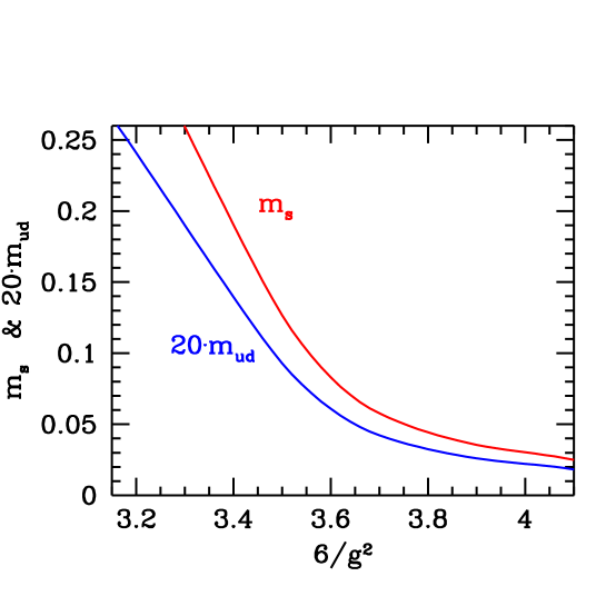
Figure 3.2: Line of constant physics defined via $m_{\pi}$, $m_{K}$ and $f_{K}$.

Once the LCP is fixed and the scale is set with the help of the three selected quantities, the expectation values of all other observables are predictions of QCD. If QCD is the correct theory of the strong interaction, these predictions should be in agreement with the corresponding experimental values (if there are any) in continuum limit. Figure 3.3 shows the $m_{K^{*}}$ mass of the $K^{*}$ meson, the $f_{\pi}$ pion decay constant and the $r_{0}$ Sommer parameter (all normalized by $f_{K}$ or its inverse). The results again were obtained with stout improved staggered fermions along the LCP shown on Figure 3.2. The continuum extrapolation has been carried out using the two or three finest lattice spacings. The difference of these extrapolations account for the systematic uncertainty of the results. In case of $m_{K^{*}}$ and $f_{\pi}$ we compared the results to the experimental values, while $r_{0}$ was compared to the results of the MILC collaboration [36].

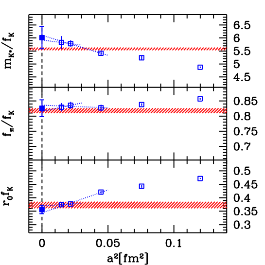
Figure 3.3: Mass of the $K^{*}$ meson, the pion decay constant and the $r_{0}$ Sommer parameter (from top to bottom). All three quantities are normalized by $f_{K}$ or its inverse. We present the results obtained at five lattice spacings, the continuum extrapolated values are also shown. The continuum extrapolations were carried out using the two or three finest lattice spacings (dashed lines). The red bands indicate the experimental values with their uncertainties in the first two cases. For $r_{0}f_{K}$ the MILC lattice result is shown.

3.3 The order of the QCD transition

The nature of the QCD transition affects our understanding of the universe’s evolution (see e.g. Ref. [42]). In a strong first order phase transition scenario the quark-gluon plasma super-cools before bubbles of hadron gas are formed. These bubbles grow, collide and merge during which gravitational waves could be produced [43]. Baryon enriched nuggets could remain between the bubbles contributing to dark matter. Since the hadronic phase is the initial condition for nucleosynthesis, the above picture with inhomogeneities could have a strong effect on it [44]. As the first order phase transition weakens, these effects become less pronounced. Recent calculations provide strong evidence that the QCD transition is an analytic transition (what we call here a crossover), thus the above scenarios -and many others- are ruled out.

There are some QCD results and model calculations to determine the order of the transition at $\mu$=0 and $\mu$$\neq$0 for different fermionic contents (c.f. [8, 3, 4, 5, 6, 7, 45, 46, 47, 48]). Unfortunately, none of these approaches can give an unambiguous answer for the order of the transition for physical values of the quark masses. The only known systematic technique which could give a final answer is lattice QCD.

When we analyze the nature and/or the absolute scale of the $T>0$ QCD transition for the physically relevant case two ingredients are quite important.

First of all, one should use physical quark masses. As Figure 1.1 shows the nature of the transition depends on the quark mass, thus for small or large quark masses it is a first order phase transition, whereas for intermediate quark masses it is an analytic crossover. Though in the chirally broken phase chiral perturbation theory provides a controlled technique to gain information for the quark mass dependence, it can not be applied for the $T>0$ QCD transition (which deals with the restoration of the chiral symmetry). In principle, the behavior of different quantities in the critical region (in the vicinity of the second order phase transition line) might give some guidance. However, a priori it is not known how large this region is. Thus, the only consistent way to eliminate uncertainties related to non-physical quark masses is to use physical quark masses (which is, of course, quite CPU demanding).

Secondly, the nature of the $T>0$ QCD transition is known to suffer from discretization errors [49, 50, 51]. Let us mention one example. The three flavor theory with a large, $a\approx 0.3$ fm lattice spacing and standard action predicts a critical pseudoscalar mass of about 300 MeV. This point separates the first order and crossover regions of Figure 1.1. If we took another discretization, with another discretization error, e.g. the p4 action and the same lattice spacing, the critical pseudoscalar mass turns out to be around 70 MeV (similar effect is observed if one used stout smearing improvement and/or finer lattices). Since the physical pseudoscalar mass (135 MeV) is just between these two values, the discretization errors in the first case would lead to a first order transition, whereas in the second case to a crossover. The only way to resolve this inconclusive situation is to carry out a careful continuum limit analysis.

Since the nature of the transition influences the absolute scale ($T_{c}$) of the transition –its value, mass dependence, uniqueness etc.– the above comments are valid for the determination of $T_{c}$, too.

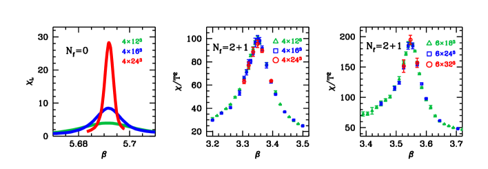
Figure 3.4: The volume dependence of the susceptibility peaks for pure SU(3) gauge theory (Polyakov-loop susceptibility, left panel) and for full QCD (chiral susceptibility on $N_{t}$=4 and 6 lattices, middle and right panels, respectively).

In order to determine the nature of the transition one should apply finite size scaling techniques for the chiral susceptibility [34]. $\chi=(T/V)\cdot(\partial^{2}\log Z/\partial m_{ud}^{2})$. This quantity shows a pronounced peak as a function of the temperature. For a first order phase transition, such as in the pure gauge theory, the peak of the analogous Polyakov susceptibility gets more and more singular as we increase the volume (V). The width scales with 1/V the height scales with volume (see left panel of Figure 3.4). A second order transition shows a similar singular behavior with critical indices. For an analytic transition (crossover) the peak width and height saturates to a constant value. That is what we observe in full QCD on $N_{t}$=4 and 6 lattices (middle and right panels of Figure 3.4). We see an order of magnitude difference between the volumes, but a volume independent scaling. It is a clear indication for a crossover. These results were obtained with physical quark masses for two sets of lattice spacings. Note, however, that for a final conclusion the important question remains: do we get the same volume independent scaling in the continuum; or we have the unlucky case what we had for 3 flavor QCD (namely the discretization errors changed the nature of the transition for the physical pseudoscalar mass case)?

One can carry out a finite size scaling analysis with the continuum extrapolated height of the renormalized susceptibility. The renormalization of the chiral susceptibility can be done by taking the second derivative of the free energy density ($f$) with respect to the renormalized mass ($m_{r}$). The logarithm of the partition function contains quartic divergences. These can be removed by subtracting the free energy at $T=0$: $f/T^{4}$ =$-N_{t}^{4}$$\cdot[\log Z(N_{s},N_{t})/(N_{t}N_{s}^{3})-\log Z(N_{s0},N_{t0})/(N_{t0}N_{s0}^{3})]$. This quantity has a correct continuum limit. The subtraction term is obtained at $T$=0, for which simulations are carried out on lattices with $N_{s0}$, $N_{t0}$ spatial and temporal extensions (otherwise at the same parameters of the action). The bare light quark mass ($m_{ud}$) is related to $m_{r}$ by the mass renormalization constant $m_{r}$=$Z_{m}$$\cdot$$m_{ud}$. Note that $Z_{m}$ falls out of the combination $m_{r}^{2}$$\partial^{2}$/$\partial$$m_{r}^{2}$=$m_{ud}^{2}$$\partial^{2}$/$\partial$$m_{ud}^{2}$. Thus, $m_{ud}^{2}\left[\chi(N_{s},N_{t})-\chi(N_{s0},N_{t0})\right]$ also has a continuum limit (for its maximum values for different $N_{t}$, and in the continuum limit we use the shorthand notation $m^{2}$$\Delta\chi$).

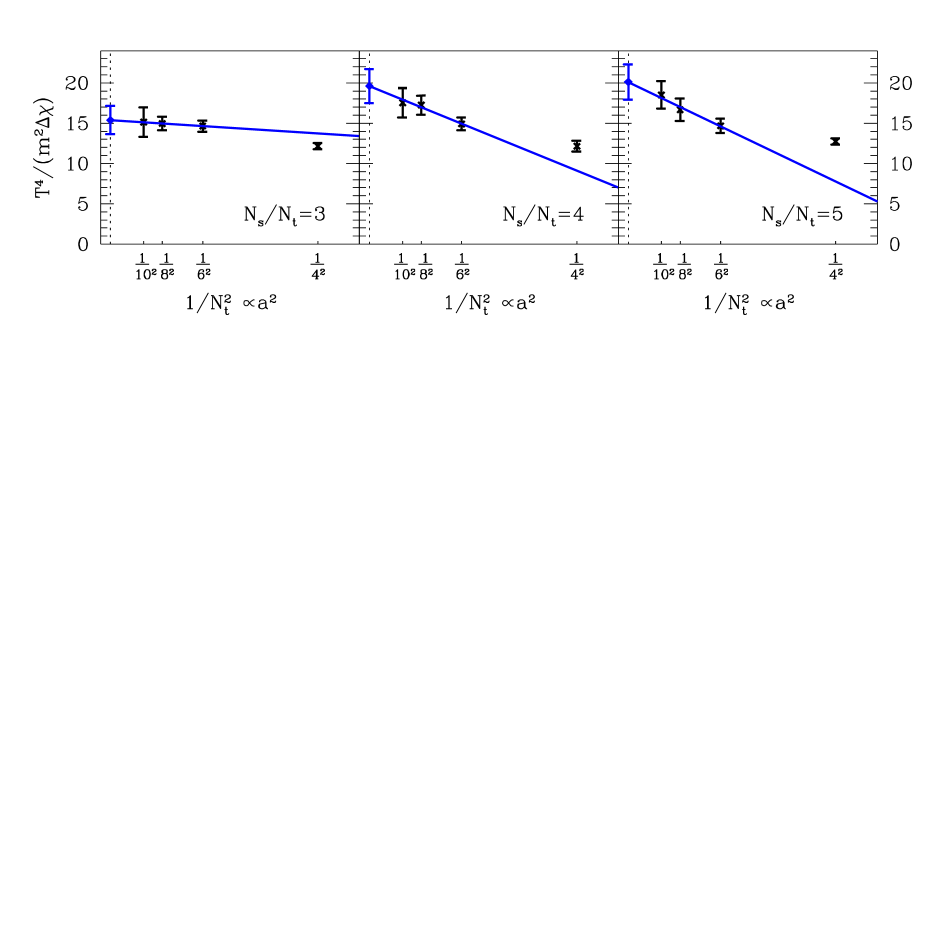
Figure 3.5: Normalized susceptibilities $T^{4}/(m^{2}\Delta\chi)$ for the light quarks for aspect ratios r=3 (left panel) r=4 (middle panel) and r=5 (right panel) as functions of the lattice spacing. Continuum extrapolations are carried out for all three physical volumes and the results are given by the leftmost blue diamonds.

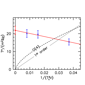
Figure 3.6: Continuum extrapolated susceptibilities $T^{4}/(m^{2}\Delta\chi)$ as a function of 1/$(T_{c}^{3}V)$. For true phase transitions the infinite volume extrapolation should be consistent with zero, whereas for an analytic crossover the infinite volume extrapolation gives a non-vanishing value. The continuum-extrapolated susceptibilities show no phase-transition-like volume dependence, though the volume changes by a factor of five. The V$\rightarrow$$\infty$ extrapolated value is 22(2) which is 11$\sigma$ away from zero. For illustration, we fit the expected asymptotic behaviour for first-order and O(4) (second order) phase transitions shown by dotted and dashed lines, which results in chance probabilities of $10^{-19}$ ($7\times 10^{-13}$), respectively.

In order to carry out the finite volume scaling in the continuum limit three different physical volumes were taken. For these volumes the dimensionless combination $T^{4}/m^{2}\Delta\chi$ was calculated at 4 different lattice spacings: 0.3 fm was always off, otherwise the continuum extrapolations could be carried out. Figure 3.5 shows these extrapolations. The volume dependence of the continuum extrapolated inverse susceptibilites is shown on Figure 3.6.

The result is consistent with an approximately constant behaviour, despite the fact that there was a factor of 5 difference in the volume. The chance probabilities, that statistical fluctuations changed the dominant behaviour of the volume dependence are negligible. As a conclusion we can say that the staggered QCD transition at $\mu=0$ is a crossover.

3.4 The transition temperature

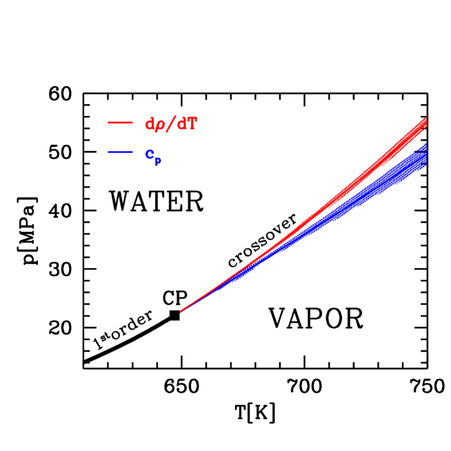
Figure 3.7: The water-vapor phase diagram.

An analytic crossover, like the QCD transition has no unique $T_{c}$. A particularly nice example for that is the water-vapor transition (c.f. Figure 3.7). Up to about 650 K the transition is a first order one, which ends at a second order critical point. For a first or second order phase transition the different observables (such as density or heat capacity) have their singularity (a jump or an infinitely high peak) at the same pressure. However, at even higher temperatures the transition is an analytic crossover, for which the most singular points are different. The blue curve shows the peak of the heat capacity and the red one the inflection point of the density. Clearly, these transition temperatures are different, which is a characteristic feature of an analytic transition (crossover).

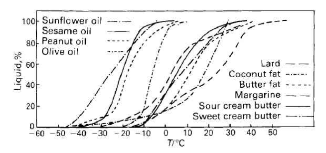
Figure 3.8: Melting curves of different natural fats.

There is another –even more often experienced– example for broad transitions, namely the melting of butter. As we know the melting of ice shows a singular behavior. The transition is of first order, there is only one value of the temperature at which the whole transition takes place at 0^oC (for 1 atm. pressure). Melting of butter shows analytic behaviour. The transition is a broad one, it is a crossover (c.f. Figure 3.8 for the melting curves of different natural fats).

Since we have an analytic crossover also in QCD, we expect very similar temperature dependence for the quantities relevant in QCD (e.g. chiral condensate, strange quark number susceptibility or Polyakov loop).

There are three lattice results on $T_{c}$ in the literature based on large scale calculations. The MILC collaboration studied the unrenormalized chiral susceptibility [52]. The possibility of different quantities leading to different $T_{c}$’s was not discussed. They used $N_{t}$=4,6 and 8 lattices, but the light quark masses were significantly higher than their physical values. The lightest ones were set to 0.1$\cdot m_{s}$. A combined chiral and continuum extrapolation was used to reach the physical point. Furthermore, they used the non-exact R algorithm. Their result is $T_{c}=169(12)(4)$ MeV, where the first error comes from the finite $T$ runs, whereas the second one from the scale setting.

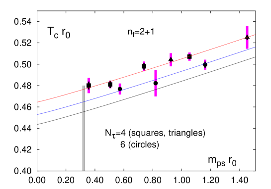
Figure 3.9: $T_{c}\cdot r_{0}$ determined by the RBC-Bielefeld collaboration [33]. Squares and triangles correspond to two slightly different strange quark masses on $N_{t}=4$, while circles show $N_{t}=6$ results. The red and blue lines show the chiral extrapolations at these lattice spacings and the black line is the continuum estimate. The vertical line indicates the physical point.

The RBC-Bielefeld collaboration has published results obtained from $N_{t}=4$ and 6 lattices [33]. They have ongoing investigations with $N_{t}=8$. They use almost physical quark masses on $N_{t}=4$ and somewhat higher on $N_{t}=6$. They study the unrenormalized chiral susceptibility and the Polyakov-loop susceptibility. They claim that both quantities give the same $T_{c}$. Figure 3.9 shows their chiral extrapolation for their two lattice resolutions. Their result is $T_{c}=192(7)(4)$ MeV, where the first error is the statistical one and the second is the systematic estimate coming from the different extrapolations.

The Wuppertal-Budapest group investigated three different quantities: the renormalized chiral susceptibility, the renormalized Polyakov-loop and the quark number susceptibility. The transition temperature obtained from the chiral susceptibility was found to be significantly smaller than the ones given by the other two quantities.

Figure 3.10: Temperature dependence of the renormalized chiral susceptibility ($m^{2}\Delta\chi/T^{4}$), the strange quark number susceptibility ($\chi_{s}/T^{2}$) and the renormalized Polyakov-loop ($P_{R}$) in the transition region. The different symbols show the results for $N_{t}=6,8$ and $10$ lattice spacings (empty boxes for $N_{t}=6$, filled and open circles for $N_{t}=8$ and $10$). The vertical bands indicate the corresponding transition temperatures and their uncertainties coming from the T$\neq$0 analyses. This error is given by the number in the first parenthesis, whereas the error of the overall scale determination is indicated by the number in the second parenthesis. The orange bands show the continuum limit estimates for the three renormalized quantities as a function of the temperature with their uncertainties.

The upper panel of Figure 3.10 shows the temperature dependence of the renormalized chiral susceptibility for different temporal extensions ($N_{t}$=6, 8 and 10). The $N_{t}=4$ results are not yet in the scaling region, thus they are not plotted. For small enough lattice spacings, thus close to the continuum limit, these curves should coincide. The two smallest lattice spacings ($N_{t}=8$ and $10$) are already consistent with each other, suggesting that they are also consistent with the continuum limit extrapolation (indicated by the orange band). The curves exhibit pronounced peaks. We define the transition temperatures by the position of these peaks. The left panel of Figure 3.11 shows the transition temperatures in physical units for different lattice spacings obtained from the chiral susceptibility. As it can be seen $N_{t}$=6, 8 and 10 are already in the scaling region, thus a safe continuum extrapolation can be carried out. The T=0 simulations resulted in a $2\%$ error on the overall scale. The final result for the transition temperature based on the chiral susceptibility reads:

$$T_{c}(\chi_{\bar{\psi}\psi})=151(3)(3){\rm~{}MeV},$$ (3.4)

where the first error comes from the T$\neq$0, the second from the T=0 analyses.

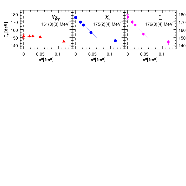
Figure 3.11: Continuum limit of the transition temperatures obtained from the renormalized chiral susceptibility ($m^{2}\Delta\chi/T^{4}$), strange quark number susceptibility ($\chi_{s}/T^{2}$) and renormalized Polyakov-loop ($P_{R}$).

For heavy-ion experiments the quark number susceptibilities are quite useful, since they could be related to event-by-event fluctuations. The second transition temperature is obtained from the strange quark number susceptibility, which is defined via [52]

$$\frac{\chi_{s}}{T^{2}}=\frac{1}{TV}\left.\frac{\partial^{2}\log Z}{\partial\mu_{s}^{2}}\right|_{\mu_{s}=0},$$ (3.5)

where $\mu_{s}$ is the strange quark chemical potential (in lattice units). Quark number susceptibilities have the convenient property, that they automatically have a proper continuum limit, there is no need for renormalization.

The middle panel of Figure 3.10 shows the temperature dependence of the strange quark number susceptibility for different temporal extensions ($N_{t}$=6, 8 and 10). As it can be seen, the two smallest lattice spacings ($N_{t}=8$ and $10$) are already consistent with each other, suggesting that they are also consistent with the continuum limit extrapolation. This feature indicates, that they are closer to the continuum result than our statistical uncertainty.

The transition temperature can be defined as the peak in the temperature derivative of the strange quark number susceptibility, that is the inflection point of the susceptibility curve. The middle panel of Figure 3.11 shows the transition temperatures in physical units for different lattice spacings obtained from the strange quark number susceptibility. As it can be seen $N_{t}$=6, 8 and 10 are already in the $a^{2}$ scaling region, thus a safe continuum extrapolation can be carried out. The continuum extrapolated value for the transition temperature based on the strange quark number susceptibility is significantly higher than the one from the chiral susceptibility. The difference is 24(4) MeV. For the transition temperature in the continuum limit one gets:

$$T_{c}(\chi_{s})=175(2)(4){\rm~{}MeV},$$ (3.6)

where the first (second) error is from the T$\neq$0 (T=0) temperature analysis. Similarly to the chiral susceptibility analysis, the curvature at the peak can be used to define a width for the transition.

$$\Delta T_{c}(\chi_{s})=42(4)(1){\rm~{}MeV}.$$ (3.7)

In pure gauge theory the order parameter of the deconfinement transition is the Polyakov-loop:

$$P=\frac{1}{N_{s}^{3}}\sum_{\bf x}{\rm tr}[U_{4}({\bf x},0)U_{4}({\bf x},1)\dots U_{4}({\bf x},N_{t}-1)].$$ (3.8)

P acquires a non-vanishing expectation value in the deconfined phase, signaling the spontaneous breakdown of the Z(3) symmetry. When fermions are present in the system, the physical interpretation of the Polyakov-loop expectation value is more complicated. However, its absolute value can be related to the quark-antiquark free energy at infinite separation:

$$|\langle P\rangle|^{2}=\exp(-\Delta F_{q\bar{q}}(r\to\infty)/T).$$ (3.9)

$\Delta F_{q\bar{q}}$ is the difference of the free energies of the quark-gluon plasma with and without the quark-antiquark pair.

The absolute value of the Polyakov-loop vanishes in the continuum limit. It needs renormalization. This can be done by renormalizing the free energy of the quark-antiquark pair [53]. Note, that QCD at T$\neq$0 has only the ultraviolet divergencies which are already present at T=0. In order to remove these divergencies at a given lattice spacing a simple renormalization condition can be used[54]:

$$V_{R}(r_{0})=0$$ (3.10)

with $r_{0}=0.46$ fm, where the potential is measured at T=0 from Wilson-loops. The above condition fixes the additive term in the potential at a given lattice spacing. This additive term can be used at the same lattice spacings for the potential obtained from Polyakov loops, or equivalently it can be built into the definition of the renormalized Polyakov-loop.

$$|\langle P_{R}\rangle|=|\langle P\rangle|\exp(V(r_{0})/(2T)),$$ (3.11)

where $V(r_{0})$ is the unrenormalized potential obtained from Wilson-loops.

The lower panel of Figure 3.10 shows the temperature dependence of the renormalized Polyakov-loops for different temporal extensions ($N_{t}$=6, 8 and 10). The two smallest lattice spacings ($N_{t}=8$ and $10$) are approximately in 1-sigma agreement (our continuum limit estimate is indicated by the orange band).

Similarly to the strange quark susceptibility case the transition temperature is defined as the peak in the temperature derivative of the Polyakov-loop, that is the inflection point of the Polyakov-loop curve. The right panel of Figure 3.11 shows the transition temperatures in physical units for different lattice spacings obtained from the Polyakov-loop. As it can be seen $N_{t}$=6, 8 and 10 are already in the scaling region, thus a safe continuum extrapolation can be carried out. The continuum extrapolated value for the transition temperature based on the renormalized Polyakov-loop is 25(4) MeV higher than the one from the chiral susceptibility. For the transition temperature in the continuum limit one gets:

$$T_{c}(P)=176(3)(4){\rm~{}MeV},$$ (3.12)

where the first (second) error is from the T$\neq$0 (T=0) temperature analysis. The width of the transition is

$$\Delta T_{c}(P)=38(5)(1){\rm~{}MeV}.$$ (3.13)

Note that the renormalized chiral susceptibility used above to define $T_{c}$ was normalized by $T^{4}$. Due to the broadness of the peak a normalization by $T^{2}$ (which is applied by the other collaborations) would increase $T_{c}$ by about 10 MeV. This means that the Wuppertal-Budapest result on the chiral susceptibility is consistent with the MILC result. There is however a significant inconsistency with the RBC-Bielefeld result. What are the differences between the two analyses and how do they contribute to the 40 MeV discrepancy? The most important contributions to the discrepancy are shown by Figure 3.12. The first difference is the different normalization of the chiral susceptibility mentioned before. This may account for $\approx 10$ MeV difference. The overall errors can be responsible for another 10 MeV. The origin of the remaining 20 MeV is somewhat more complicated. One possible explanation can be summarized as follows. In Ref. [33] only $N_{t}$=4 and 6 were used, which correspond to lattice spacings a=0.3 and 0.2 fm, or $a^{-1}$=700MeV and 1GeV. These lattices are quite coarse and it seems to be obvious, that no unambiguous scale can be determined for these lattice spacings. The overall scale in Ref. [33] was set by $r_{0}$ and no cross-check was done by any other quantity independent of the static potential (e.g. $f_{k}$). This choice might lead to an ambiguity for the transition temperature, which is illustrated for the Wuppertal-Budapest data on Figure 3.13. Using only $N_{t}$=4 and 6 the continuum extrapolated transition temperatures are quite different if one took $r_{0}$ or $f_{K}$ to determine the overall scale. This inconsistency indicates, that these lattice spacing are not yet in the scaling region (similar ambiguity is obtained by using the p4 action of [33]). Having $N_{t}$=4,6,8 and 10 results this ambiguity disappears (as usual $N_{t}$=4 is off), these lattice spacings are already in the scaling region (at least within the present accuracy).

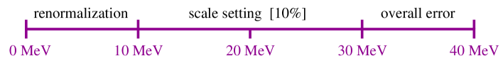
Figure 3.12: Possible contributions to the 40 MeV difference between the results of Refs. [55] and [33].

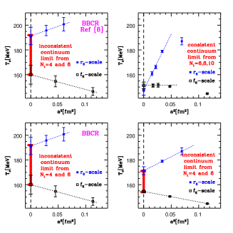
Figure 3.13: Continuum extrapolations based on $N_{t}$=4 and 6 (left panel: inconsistent continuum limit) and using $N_{t}$=6,8 and 10 (right panel: consistent continuum limit).

The ambiguity related to the inconsistent continuum limit is unphysical, and it is resolved as we approach the continuum limit (c.f. Figure 3.13). The differences between the $T_{c}$ values for different observables are physical, it is a consequence of the crossover nature of the QCD transition.

3.5 Equation of state

In the previous sections we discussed the nature of the QCD transition and its characteristic scale. Now we extend the analysis to cover a larger temperature range [31]. In order to describe the equilibrium properties of the quark-gluon plasma and/or the hadronic phase one has to determine the equation of state. The equation state describes the functional relationship between various thermodynamical quantities. The most common way to start with is to calculate the pressure as a function of the temperature. Using this function the temperature dependence of other quantities can be determined (energy density, entropy density, speed of sound etc.), too.

Several recent papers discuss the equation of state. For the pure SU(3) theory several lattice actions were used [56, 57, 58]. In all of these cases the equation of state was given upto about $4T_{c}$. There are few percent differences between the various results, however, these differences can be traced back to the scale setting problem. Note, that defining a scale in physical units is in principle impossible for the pure SU(3) theory, experimentally measurable quantities should be compared with results obtained in full QCD. Thus, for the pure SU(3) case only dimensionless combinations (e.g. ratios) can be considered as predictions (dimensionless combinations can be obtained also in full QCD). It is worth mentioning that until recently it was technically impossible to calculate the equation of state to much higher temperatures ($T\gg T_{c}$). In a recent work this old problem was solved[59].

There are several full QCD results for the equation of state, though none of them can be considered as full result. Unimproved dynamical results in the staggered formalism were published [60, 61]. Another important result used ${\cal O}(a)$ improved Wilson fermions. As for the transition temperature, also for the equation of state improved staggered fermions provide the fastest way to approach the physical quark mass and continuum limits. The most important results are obtained by the p4fat3 action (see e.g. [62, 63]). Other improved staggered results can be found for the ASQTAD action [64] and for the stout-smeared action [31]. It is illustrative to summarize the uncertainties of [62] (many of them were cured in their –and other’s– later publications). This sort of summary nicely shows how uncertainties are eliminated through computational and technical progress.

(1) It is of particular importance to use physical quark masses both at T=0 and T>0. Until now the only published work which used physical quark masses are the one with stout-smeared improvement [31]. In earlier works [62] pion masses of e.g. 600 MeV were used. Since the physical pion mass is smaller than the transition temperature, it is obviously important to use pion contributions with the proper Boltzmann weights.

(2) In order to approach the continuum limit one has to use small enough lattice spacing. At least $N_{t}$=6 and 8 is needed (as we discussed earlier e.g. $N_{t}$=4 can not be used to set the scale reliably).

(3) In the staggered formalism one has instead of three degenerate pseudo-Goldstone bosons ($\pi^{+}$, $\pi^{-}$ and $\pi^{0}$) only one. The others are separated from this single one by a gap, which can be as large as several hundred MeV. The size of the gap depends on the choice of the action and on the lattice spacing. As we have seen the stout-smeared improvement is the best choice to reduce this taste symmetry violation.

(4) In several studies [62, 64] an inexact Monte-Carlo technique was used, the so-called R-algorithm. Recently, an exact algorithm appeared on the market, which allows to perform 2+1 flavour staggered simulations (RHMC algorithm). The first large scale analysis, which used an exact algorithm for staggered thermodynamics was Ref. [31], which was then followed by [63].

(5) For a long time all staggered analyses used the non-LCP approach. In this approximation there is a serious mismatch between the pion masses. E.g. if one cooled down the analyzed systems at $0.8T_{c}$ and at $3.2T_{c}$ to vanishing temperature, the pion mass would be twice as large for the second system. This is clearly un-physical. The first work with the the proper line of constant physics was Ref. [31] (using the heavy quark potential to set the relative scales), which was then followed by [64, 63].

For large homogeneous systems the pressure is proportional to the free-energy density, which is the logarithm of the partition function $Z$.

$$p=\frac{T}{V}\ln Z.$$ (3.14)

On a space-time lattice one determines the dimensionless $pa^{4}$ combination.

$$pa^{4}=\frac{1}{N_{t}N_{s}^{3}}\ln Z.$$ (3.15)

Since the free energy has divergent terms, when we approach the continuum limit, one has to renormalize. As it was done earlier, this renormalization can be achieved by subtracting the T=0 term. To that end one has to carry out simulations on $T=0$ lattices. The partition function on T=0 lattices will be denoted by $Z_{0}$. The size of this T=0 lattice is $N_{s0}^{3}\cdot N_{t0}$. The renormalized pressure is usually normalized by $T^{4}$ which leads to a dimensionless combination

$$\frac{p_{R}}{T^{4}}=N_{t}^{4}\left[\frac{1}{N_{t}N_{s}^{3}}\ln Z-\frac{1}{N_{t0}N_{s0}^{3}}\ln Z_{0}\right].$$ (3.16)

In the rest of this review we omit the index $R$, since we use only renormalized quantities. This renormalization prescription automatically fulfills the $p(T=0)=0$ condition. It is worth mentioning that for a fixed lattice spacing $a$ the weight of the terms proportional to $1/a^{2}$ (thus the diverging term) is much larger for the pressure than for the chiral susceptibility. It is particularly true for large temperatures. Thus we have to determine the difference between two almost equal numbers, which needs high numerical accuracy. This is one of the most important reason, why only $N_{t}$=4 and 6 published results available for the pressure, whereas for the transition temperature there are $N_{t}$=4,6,8 and 10 published results, too. Another reason for the different levels of results is related to the lattice spacings. For large temperatures even the $N_{t}$=4 analyses need small lattice spacings and relatively large T=0 lattices. E.g. on $N_{t}=4$ lattices at $T=2.5T_{c}$ one needs the same $T=0$ lattices as for the $T_{c}$ determination on $N_{t}=10$ lattices. Quite recently, a new method appeared, which eliminates this difficulty and provides a renormalization by using T>0 lattice simulations[59].

As usual for a fixed $N_{t}$ we tune the temperature by changing the gauge coupling $\beta$. In order to avoid any non-physical mismatch we keep the system along the LCP. Thus, determining $\ln Z$ and $\ln Z_{0}$ along the proper LCP-defined ($\beta,am_{q}$) line gives us the pressure (for simplicity $m_{q}$ denotes both the light and the strange quark masses). We discussed the simulation algorithms based on importance sampling in Chapter 2.4. Unfortunately, these algorithms are not able to directly provide $Z$ or $\ln Z$, only derivatives of the partition functions can be determined. Therefore, the most straightforward technique is the integral method [65]. The pressure is obtained as an integral of its derivatives along a line in the multi-dimensional $(\beta,am_{q})$ space.

$$\frac{p}{T^{4}}=N_{t}^{4}\int^{(\beta,am_{q})}_{(\beta_{0},am_{q0})}d(\beta,am_{q})\left[\frac{1}{N_{t}N_{s}^{3}}\left(\begin{array}[]{c}{\partial\ln Z}/{\partial\beta}\\ {\partial\ln Z}/{\partial(am_{q})}\end{array}\right)-\right.$$ (3.19)

$$\left.\frac{1}{N_{t0}N_{s0}^{3}}\left(\begin{array}[]{c}{\partial\ln Z_{0}}/{\partial\beta}\\ {\partial\ln Z_{0}}/{\partial(am_{q})}\end{array}\right)\right].$$ (3.22)

Since the integrand is the gradient of the pressure, the value of the integral is independent of the integration path. Nevertheless, it is useful to integrate along the line of constant physics. In this case the endpoints of the integration paths will be just on the LCP, which we need. As we will see later a slightly modified path is even more appropriate (in order to carry out the chiral extrapolations at $T=0$).

The lower end of the integration path should be chosen to ensure zero pressure. This goal can be reached by using temperatures well below the $T_{c}$. It is straightforward to calculate the derivatives, they are just the expectation values of the various terms of the staggered fermion and gauge actions (2.9,2.6).

$$\frac{\partial\ln Z}{\partial\beta}=\left<-S_{g}/\beta\right> \frac{\partial\ln Z}{\partial(am_{ud})}=\left<\bar{\psi}\psi_{ud}\right> \frac{\partial\ln Z}{\partial(am_{s})}=\left<\bar{\psi}\psi_{s}\right>.$$ (3.23)

The pressure can be written as

$$\frac{p}{T^{4}} = N_{t}^{4}\int^{(\beta,am_{ud},am_{s})}_{(\beta_{0},am_{ud0},am_{s0})}d(\beta,am_{ud},am_{s})\times$$ (3.30)

$$\left[\frac{1}{N_{t}N_{s}^{3}}\left(\begin{array}[]{c}\langle{\rm-S_{g}/\beta}\rangle\\ \langle\bar{\psi}\psi_{ud}\rangle\\ \langle\bar{\psi}\psi_{s}\rangle\end{array}\right)-\frac{1}{N_{t0}N_{s0}^{3}}\left(\begin{array}[]{c}\langle{\rm-S_{g}/\beta}\rangle_{0}\\ \langle\bar{\psi}\psi_{ud}\rangle_{0}\\ \langle\bar{\psi}\psi_{s}\rangle_{0}\end{array}\right)\right].$$

Here $\left<\dots\right>_{0}$ denotes the expectation values calculated on $T=0$ lattices.

The integral method was originally introduced for pure gauge theories. Since these theories –at least in their simplest formulations– have only one parameter $\beta$ the pressure can be given by an integral over $\beta$. Earlier staggered works used the same strategy, which –as we pointed out already– does not correspond the physical LCP. The proper solution is to use the line of constant physics and avoid any mismatch of the spectrum.

The above formulas give the pressure as a function of the gauge coupling $\beta$. Clearly, one needs $p$ as a function of the temperature. To that end we need the $\beta$ dependence of the lattice spacing $a$. This can be the dependence in absolute units (MeV) or in relative units ($T/T_{c}$). The relative units are somewhat easier to determine, e.g. one can calculate the static potential for each $\beta$ and compare them directly (or compare some characteristic points of them $r_{0}$ or $r_{1}$). In order to give the lattice spacing in physical units one has to insert the physical value of $r_{0}$ or $r_{1}$ (unfortunately, –as it was discussed earlier– they are not very precisely known).

The energy density ($\epsilon$), the entropy density ($s$) and the speed of sound can be derived using the pressure and various thermodynamic relations:

$$\epsilon=T(\partial p/\partial T)-p, s=(\epsilon+p)T, c_{s}^{2}=\frac{dp}{d\epsilon}.$$ (3.31)

The derivatives of $p$ can be calculated numerically.

There is another popular method to determine the energy density. The energy density can be written as $\epsilon(T)={T^{2}}/{V}{\partial{\log Z}}/{\partial{T}}$. Using this form and the relationship between the temperature, volume and the lattice spacing one can easily show that

$$\frac{\epsilon-3p}{T^{4}}=-\frac{N_{t}^{3}}{N_{s}^{3}}a\frac{d(\log Z)}{da}.$$ (3.32)

Thus, the expression $\epsilon-3p$ can be directly determined by using the total derivative with respect to the lattice spacing. There are different names for this quantity, Sometimes it is called “interaction measure” (at very high temperatures its value tends to zero, reflecting the non-interactive feature of the system), or “trace anomaly”. The above total derivative can be written as a derivative with respect to $\beta$ and the quark masses (one uses the chain rule). Renormalization is carried out analogously as in the case of the pressure. Adding three times the pressure to the trace anomaly gives the energy density.

The energy density can be also obtained from the pressure (3.31). This choice is particularly useful, if one uses larger than physical quark masses at $T=0$ and uses chiral perturbation theory for the extrapolation to the physical value. The form of the chiral extrapolation is not known for all relevant quantities. For the chiral condensate $\left<\bar{\psi}\psi\right>$, which is needed for the pressure, the leading form is linear in the quark masses. The precise extrapolation form for the for the gauge action or for the trace anomaly is not known. Thus, in order to determine the pressure one integrates along an LCP defined by a larger quark mass, after which the integration path is at fixed $\beta$. Along this last path the integrand is the chiral condensate, for which chiral perturbation theory predicts the functional form. Using this technique one can avoid uncertainties in the chiral extrapolation.

All three collaborations have results on the equation of state. The Wuppertal-Budapest group used physical quark masses and $N_{t}=$4,6 lattices [31]. The result is shown on Figure 3.14. The MILC and RBC-Bielefeld collaborations used somewhat higher quark masses. Their results are shown on Figures 3.15 and 3.16. The RBC-Bielefeld collaboration also has a few points on $N_{t}=8$ lattices.

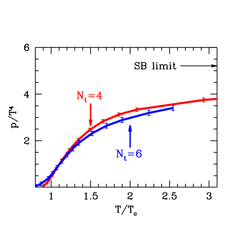
Figure 3.14: The pressure determined by the Wuppertal-Budapest group [31].

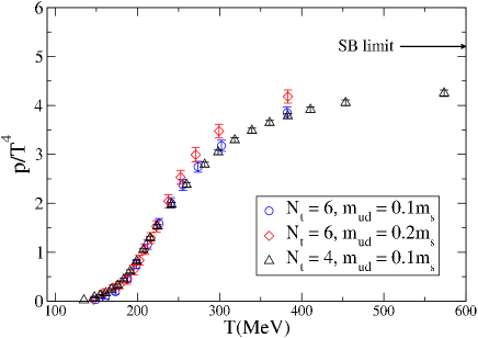
Figure 3.15: The pressure determined by the MILC collaboration [64].

Figure 3.16: Pressure and energy density determined by the RBC-Bielefeld collaboration [63].

3.6 Note added in proof

Since the submission of this review both the Wupperal-Budapest and the HotQCD collaborations improved on their data. The Wuppertal-Budapest group used physical quark masses also for the $T=0$ simulations and took even finer lattice spacings ($N_{t}=12$ and $N_{t}=16$ at one point) at finite temperature [66]. The $T_{c}$ values remained consistent with the previous results. The HotQCD collaboration uses two lattice actions (asqtad and p4) and they extended their simulations to $N_{t}=8$ lattices [67]. They also determined the equation of state on $N_{t}=8$ lattices. The results of the two groups remained inconsistent.

A possible reason for the discrepancy could be the uncertainty coming from the scale setting. Different quantities can be used to set the lattice spacing and the results should not depend on this choice. It is important to check that the $T=0$ simulations, which are needed for scale setting, are in the scaling regime. For staggered fermions, due to the taste symmetry violation at finite lattice spacings, this is particularly important. The Wuppertal-Budapest group has carried out such an analysis.

Figure 3.17 shows the masses of the $\Omega$ baryon, $\phi(1020)$ meson and $K^{*}(892)$ meson as well as the ratio of the quark masses and $f_{K}/f_{\pi}$ obtained from $T=0$ simulations of the Wuppertal-Budapest collaboration [66]. The agreement to the experimental values indicates that the finite temperature results are independent of which quantity ($\Omega$, $K^{*}$ or $\Phi$ mass, or the pion decay constant) is chosen for scale setting.

On Figure 3.18(left) the renormalized chiral condensate ($\Delta_{ls}$) is shown as a function of the temperature. We used the Wuppertal-Budapest data as well as the $N_{t}=8$ data of the ’hotQCD’ collaboration from [68]. We can see a huge disagreement between the curves in the transition regime. The shift between the curves of the different groups is in the order of $35$ MeV.

The strange quark number susceptibility is shown in Figure 3.18(right). The $N_{t}=12$ data of the Wuppertal-Budapest group is shown with one additional $N_{t}=16$ point at a high temperature. The comparison with the results of the ’hotQCD’ collaboration (see Reference [69]) brings us to a similar conclusion as for the chiral condensate. Around the transition point there is an approximately $20$ MeV shift between the results of the two groups.

The most recent $T_{c}$ values published by the different groups are given in Table 3.1. The latest results of the Wuppertal-Budapest group are consistent with the ones from 2006. The small difference comes from the fact that the experimental value of $f_{K}$ has changed slightly since 2006. The discrepancy between the Wuppertal-Budapest results and the ’HotQCD’ ones is still present and has to be resolved by future work.

	$\Delta\chi_{\bar{\psi}\psi}/T^{4}$	$\Delta\chi_{\bar{\psi}\psi}/T^{2}$	$\Delta\chi_{\bar{\psi}\psi}$	$\Delta_{l,s}$	L	$\chi_{s}$
Wuppertal-Budapest ’09	146(2)(3)	152(3)(3)	157(3)(3)	155(2)(3)	170(4)(3)	169(3)(3)
Wuppertal-Budapest ’06	151(3)(3)	-	-	-	176(3)(4)	175(2)(4)
RBCBC (ref. [33])	-	192(4)(7)	-	-	192(4)(7)	-

Table 3.1: Continuum extrapolated transition temperatures at the physical point for different observables and in different works. The first three columns give $T_{c}$ obtained from the chiral susceptibility using different normalizations. The other three columns give $T_{c}$ from the renormalized chiral condensate, renormalized Polyakov-loop and the strange quark number susceptibility.

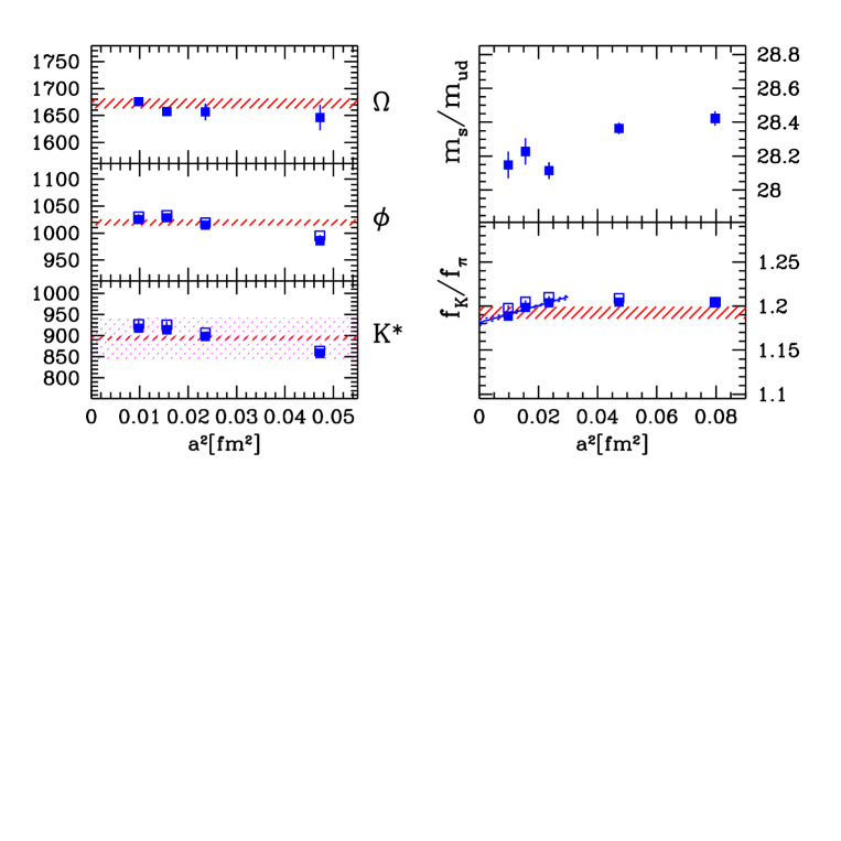
Figure 3.17: Left panel: masses of $\Omega$ baryon, $\phi(1020)$ meson and $K^{*}(892)$ meson in MeV on our four finest lattices as a function of the lattice spacing squared. Right panel: quark mass ratio and $f_{K}/f_{\pi}$ for all five ensembles. See text for a detailed explanation.

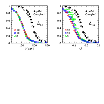
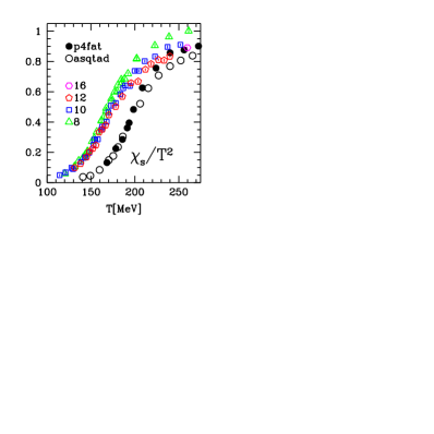
Figure 3.18: Left panel: renormalized chiral condensate as a function of the temperature. The triangles, squares and pentagons correspond to $N_{t}=6,8$ and 10 results of the Wuppertal-Budapest group, respectively. The ’HotQCD’ results are also shown by the closed and open circles. Right panel: strange quark number susceptibility.

4 Finite chemical potential

In the last part of this review we discuss non-vanishing baryonic chemical potentials. These studies are extremely difficult, since the infamous sign-problem spoils any method based on importance sampling. Since the phase space is huge all lattice calculations use importance sampling. Thus for non-vanishing baryonic chemical potentials no direct simulations are possible. Until recently (till 2001) the most advocated method was the Glasgow-method [70], which was in principle theoretically correct, unfortunately only in the infinite statistics limit. As it turned out even after producing several million configurations on tiny lattices the method did not work in practice. The reasons for this unlucky situation will be discussed later. There were several model studies, for systems other than QCD. Though these studies might give some insight to the real question (full QCD) they are of very limited practical use, therefore we do not discuss them any more.

In the following we show how one can introduce the baryonic chemical potential in lattice field theory and illustrate the infamous sign problem. After that we show the first method, which opened the way for quantitative predictions in full QCD at non-vanishing baryonic chemical potentials (overlap improving multi-parameter reweighting). This method is still one of the most accurate techniques, for many questions probably the best one we know. Since then several other techniques were suggested, which we also discuss briefly.

Later we will discuss the potentials and goals of the forthcoming years. As we will see, it is not yet possible to determine the continuum limit at non-vanishing baryonic chemical potentials. Thus, we will use non-improved staggered (2.9) and Wilson (2.5) actions. Once the techniques are more established and more CPU power is available than today, one should systematically analyze actions and decide which one is the least CPU-demanding when we approach the continuum limit.

4.1 Chemical potential on the lattice

In continuum we use the grand canonical potential to treat non-zero chemical potential and use the corresponding $\mu N$ term (N is the particle number). In the Euclidean lattice formulation the particle number is proportional to $\bar{\psi}\gamma_{4}\psi$. Thus, the most obvious solution for non-zero chemical potentials would be to add a $\mu\sum_{x}\bar{\psi}\gamma_{4}\psi$ term to the action. It is easy to show that this choice leads to a quadratic divergence. Note, however, that a term of the form $\mu\sum_{x}\bar{\psi}\gamma_{4}\psi$ corresponds to a constant purely imaginary vector potential. Since we describe gauge fields by link variables, it is straightforward to define non-vanishing chemical potentials also by link variables [71]. Based on these ideas it is clear, how to introduce $\mu$ on the lattice. We multiply the forward timelinks $U_{x;4}$ by $e^{a\mu}$ and the the backward timelinks $U^{\dagger}_{x;4}$ by $e^{-a\mu}$, otherwise the form of the action remains the same. The staggered action (2.9) reads:

$$S_{f,\rm{staggered}}(\mu)=\sum_{x} \left[am\bar{\chi}\chi+\frac{1}{2}\sum_{\nu=1\dots 3}\alpha_{x;\nu}\left(\bar{\chi}_{x}U_{x;\nu}\chi_{x+a\hat{\nu}}-\bar{\chi}_{x}U^{\dagger}_{x-a\hat{\nu};\nu}\chi_{x-a\hat{\nu}}\right)+\right.$$ (4.1)

$$\alpha_{x;4}\left.\left(\bar{\chi}_{x}U_{x;4}e^{a\mu}\chi_{x+a\hat{4}}-\bar{\chi}_{x}U^{\dagger}_{x-a\hat{4};4}e^{-a\mu}\chi_{x-a\hat{4}}\right)\right].$$

For several quark fields (flavours) one has to introduce the chemical potentials for each flavours, they can be the same or they can be different. In the following we set the chemical potential of the strange quark to zero, whereeas the up and down quarks have the same chemical potentials. This choice is motivated by the physical conditions in heavy ion collisions (the initial state has zero strangeness, through the strong interactions only strange-antistrange pairs can be produced –which does not change the total strangeness, the only way to produce non-vanishing strangeness is through the weak interaction, which is subdominant). Baryons with three light quarks have a baryonic chemical potential $\mu_{B}$, which is three times the chemical potential of the light quarks.

For some questions one introduces the isospin chemical potential. To that end the up and down quarks have opposite $\mu$ values. One can study systems with non-vanishing isospin chemical potentials by using standard importance sampling methods, since the sign problem is not present in this case. In the rest of this review we want to deal with the sign problem and present various suggestions how to deal with it, therefore we do not discuss the non-vanishing isospin chemical potential any longer.

4.2 The sign problem

In section 2.4 we presented the available simulation algorithms, and discussed the necessary ingredients, particularly the positivity of the fermion determinant. At zero chemical potential this positivity is garanteed by the $\gamma_{5}$ hermiticity of the fermion matrix. Unfortunately, at non-vanishing chemical potentials the $\gamma_{5}$ hermiticity is no longer fulfilled, the fermion determinant can take complex values. The partition function and the observables are real valued, thus we can take the real part of the integrand ${\rm Re}\det Me^{-S_{g}}$. The positivity of this quantity is, however, not garanteed, it can take both positive and negative values. This is the so-called sign problem.

This feature (positive and negative signs in the integrand) has two consequences. The more serious one is the impossibility to generate configurations based on importance sampling (a function with negative values can not be interpreted as a probability distribution). The other problem is related to the cancellation due to contributions of different signs. Even if we could generate the necessary configurations the sign of ${\rm Re}\det Me^{-S_{g}}$ for the individual configurations oscillates, and there are large cancellations in the average, which reduces the numerical accuracy.

Figure 4.1: The expectation value of $\cos\phi$ as a function of $a\mu$, The phase of the fermion determinant is denoted by $\phi$.

In order to illustrate the second problem let us write the determinant as

$$\det M=\left|\det M\right|e^{i\phi}.$$ (4.2)

One can study the oscillation of the phase on a give ensemble. In order to do that we evaluate the determinant on each configuration and calculate $\cos\phi$, which appears in the real part. The average of the $\cos\phi$ factors are shown as a function of the chemical potential on Figure 4.1. The configurations were obtained on a $8^{3}\cdot 4$ lattice at vanishing chemical potential at $\beta=5.1991$ and with $am_{ud}=0.025$, $am_{s}=0.2$ quark masses. The gauge coupling was tuned to the transition point.

As it can be seen for small chemical potentials the expectation value of $\cos\phi$ can be determined quite precisely, for $a\mu\raise 1.29167pt\hbox{$>$\kern-7.5pt\raise-4.73611pt\hbox{$\sim$}}0.4$ the phase oscillation is so strong, that the average of $\cos\phi$ is consistent with zero, the sign problem became quite serious.

4.3 Multi-parameter reweighting

A simple, but powerful generalization of the Glasgow method is the overlap improving multi-parameter reweighting [72]. The partition function at finite $\mu$ can be rewritten as:

$$Z=\int{\cal D}Ue^{-S_{g}(\beta,U)}[\det M(m,\mu,U)]^{N_{f}/4}=$$

$$\int{\cal D}Ue^{-S_{g}(\beta_{0},U)}[\det M(m_{0},\mu=0,U)]^{N_{f}/4}$$ (4.3)

$$\left\{e^{-S_{g}(\beta,U)+S_{g}(\beta_{0},U)}\left[\frac{\det M(m,\mu,U)}{\det M(m_{0},\mu=0,U)}\right]^{N_{f}/4}\right\},$$

where the second line contains a positive definite action which can be used to generate the configurations and the terms in the curly bracket in the last line are taken into account as an observable. The expectation value of any observable can be then written in the form:

$$<O>_{\beta,m,\mu}=\frac{\sum O(\beta,m,\mu)w(\beta,m,\mu)}{\sum w(\beta,m,\mu)}$$ (4.4)

with $w(\beta,m,\mu)$ being the weights of the configurations defined by the curly bracket of eqn. (4.3).

The main difference from the Glasgow method is that reweighting is done not only in $\mu$ but also in the other parameters of the action (at least in $\beta$, but possibly also in $m$). This way the overlap can be improved. If the starting point ($\beta_{0},m_{0},\mu_{0}=0$) is selected to be at the $\mu=0$ transition point then a much better overlap can be obtained with transition points at higher $\mu$. A schematic figure shows the main differences between the two techniques (see Figure 4.2).

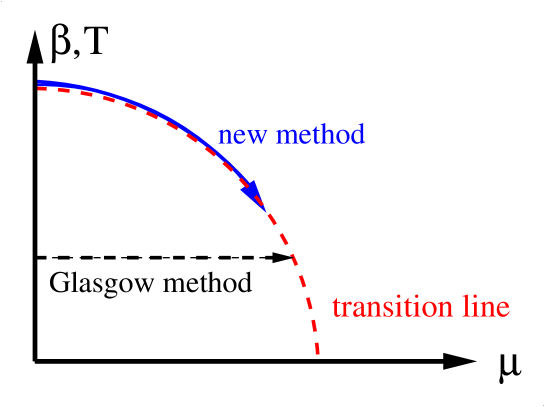
Figure 4.2: Comparison of the Glasgow method and the the new (multi-parameter reweighting) method. The Glasgow method collects an ensemble deep in the hadronic phase, attaches weights to the individual configurations and attempts to get information about the phase diagram, thus informations about configurations on the other side of the phase line. There is no overlap between the original typical configurations (hadronic phase) and the configurations of the new phase. This is the reason why the method fails. The new technique (overlap improving multi-parameter reweighting) determines the phase line in a different way. First one tunes the system to the transition point at $\mu$=0. At this point the configuration ensemble contains configurations from both phases. A simultaneous reweighting is done in $\beta$ (or in other words in the temperature) and also in $\mu$. Since we are looking for the phase line, thus for an equal “mixture” of the two phases, a careful change of the two parameters keeps the system in this mixed phase. The overlap between $\mu$=0 and $\mu\neq$0 is much better, the phase line can be determined.

Though all formulas are exact, nevertheless the practical applicability depends on the fluctuation of the weights $w(U)$. In principle there might be two difficulties. The first one is the so-called overlap problem. In order to illustrate this question we study a reweighting, for which both the simulation and the target parameters allows direct importance sampling based simulations, thus the determinants are for both ($\beta,m,\mu$) sets positive, e.g. for $\mu=0$. Since the weights are positive real numbers, importance sampling is possible. Thus, there are some smaller subsets of configurations, which are particularly important (these subsets are selected by the importance sampling procedure). This is true for both parameter sets ($\beta,m,\mu$). In practice, the simulations results in some configurations from these subsets. If the two subsets are disjoint (the typical configurations of one of the subsets are quite different than the typical configurations of the other subset) the so-called overlap problem appears. In this case assigning new weights to the configurations does not help, since the most important, typical configurations are simply missing. One of the most unconvenient features of the overlap problem is that it is very difficult to detect. Let us look at an extreme example and assume that the two subsets are very different, e.g. they correspond to different phases of the physical system. For small ensembles usually no configurations can be obtained from the other phase. The $w(U)$ will be of similar size and the result will have a artificially small statistical error. If we increase the statistics a configuration, which is just typical for the other phase, might appear. This single configuration receives a large weight and it will change and even dominate the result. Clearly, as long as our ensemble is small and no such configuration is produced, one is not aware of the overlap problem. This was exactly the most serious problem of the Glasgow method.

The other difficulty for the multy-parameter reweighting is the sign-problem. The phase of the determinant appears in the weights $w$. For large chemical potentials the sum of these complex weights can be even consistent with zero (at least for small statistics). In these cases the expression (4.4) will be practically $0/0$. This feature is fortunately signalled by the jackknife analysis, since it uses different subsamples (the cancellation in different subsemples are different, which influence the jackknife error). A large statistical error is a clear sign of the sign-problem.

4.3.1 Multi-parameter reweighting with Taylor-expansion

There is a variant of the above multi-parameter reweighting technique, which needs less computational power, particularly for large lattices, though this method contains somewhat less informations of the $\mu$ dependence. Let we discuss how it works. The use of eqn. (4.3) requires the exact calculation of determinants on each gauge configuration which is computationally expensive. Instead of using the exact formula, one can make a Taylor expansion for the determinant ratio in the weights [73] (for simplicity assuming no reweighting in the mass):

$$\ln\left[\frac{\det M(\mu)}{\det M(0)}\right]^{N_{f}/4}=\sum_{n=1}^{\infty}\frac{\mu^{n}}{n!}\frac{\partial^{n}\ln\left[\det M(0)\right]^{N_{f}/4}}{\partial\mu^{n}}\equiv\sum_{n=1}^{\infty}{R}_{n}\mu^{n}.$$ (4.5)

Taking only the first few terms of the expansion one gets an approximate reweighting formula. The advantage of this approximation is that the coefficients are derivatives of the fermion determinant at $\mu=0$, which can be well approximated stochastically. However, due to the termination of the series and the errors introduced by the stochastic evaluation of the coefficients we do not expect this method to work for as large $\mu$ values as the full technique. Indeed, it has been shown in Ref. [74] that even for very small lattices (i.e. $4^{4}$) the phase of the determinant is not reproduced by the Taylor expansion for $a\mu\geq 0.2$.

4.3.2 Simulations at imaginary $\mu$

The fermion determinant is positive definite if we use a purely imaginary chemical potential. So if the transition line $T_{c}(\mu)$ is an analytic function then we can determine it for imaginary $\mu$ values and analytically continue back to real $\mu$-s [75]. The analytic continuation is in general impossible from just a finite number of points. However, taking a Taylor expansion in $\mu$ or $\mu/T$ one gets:

$$\frac{T_{c}(\mu_{B})-T_{c}(0)}{T}=a_{2}\left(\frac{\mu_{B}}{T}\right)^{2}+a_{4}\left(\frac{\mu_{B}}{T}\right)^{4}+\dots$$ (4.6)

The coefficients $a_{i}$ can be determined from imaginary $\mu$ simulations. One simply measures $T_{c}(\mu_{I})$ for imaginary $\mu_{I}$-s and fits it with a finite order polynomial in $\mu_{I}/T$. Recently, a generalization of this method was proposed by using a more general form of the action which still preserves the positivity of the fermion determinant [76].

Recently, instead of using the grand-canonical partition function a canonical approach was also applied to study QCD at non-zero density [77, 78]. This technique involves a Fourier integral for which the fermion determinant at imaginary $\mu$ values is needed. The sign problem emerges as fluctuations during the evaluation of this Fourier integral.

4.3.3 Differences and similarities of the three techniques

Although the three described methods seem different they are essentially the same. The connection between exact reweighting and Taylor expansion is obvious: the latter is an approximation of the former, using all non-vanishing orders in the Taylor expansion gives exactly the same results as reweighting.

To see the connection between reweighting and analytic continuation is not so straightforward. Since the phase diagram for imaginary $\mu$ is fitted by a polynomial it yields the $\mu$ derivatives at $\mu=0$ (the closest point to the real $\mu$ domain, since $\mu^{2}$ is the natural variable). In this sense it should give the same results as the Taylor expansion method in the same order. Thus, for moderate $\mu$ values the imaginary $\mu$ method should also agree with exact reweighting. The agreement is demonstrated on Figure 4.3. In order to avoid difficulties when comparing different discretizations, different quark masses, different choices to transform lattice data into physical units and exact/non-exact Monte-Carlo generators we applied the three methods using identical circumstances. We took the same phase diagram as in Ref. [75] and used their determination for the curvature of the phase line. Their result is perfectly reproduced (upto four digits) by multi-parameter reweighting with full determinants and also by the Taylor technique. As the chemical potential gets larger the results start to deviate. This fact is an obvious consequence of the higher order $\mu$ terms, which are missing both from the imaginary chemical potential method and from the Taylor expansion technique.

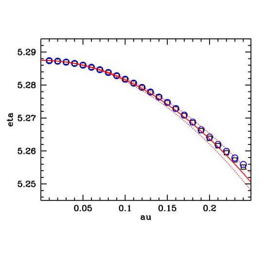
Figure 4.3: The $N_{f}=2$ phase diagram of Ref. [75] obtained via analytic continuation from imaginary $\mu$ (solid line; dotted lines show the uncertainty) and the same system calculated by exact multi-parameter reweighting (boxes) and Taylor expansion up to $\mu^{4}$ order (circles). There is a perfect agreement. To enhance the differences the results were matched at $\mu=0$ points (note, that they agree within their uncertainties). The errors are smaller than the symbol sizes.

As we mentioned previously in the case of staggered fermions a fractional power of the fermion determinant is taken in order to have less than four flavors. For $\mu>0$ this leads to an additional difficulty. The fourth root of a complex number cannot be taken unambiguously. There are several ways to circumvent this problem. It has been shown in Ref. [79] that near the continuum limit these unambiguities dissappear and a unique fourth root can be defined. It has also been argued, however, that current lattices are not yet close enough to the continuum in this sense. The procedure the authors of Ref. [79] propose does not work on todays lattices. An alternative method to choose among the Riemann leaves is given in Ref. [80] which assumes analyticity of the fourth root along the real $\mu$ axis. Close to the continuum where the procedure of Ref. [79] can be applied the two methods choose the same roots, thus they agree. Since both Taylor expansion and analytic continuation from imaginary chemical potentials implicitly assume analyticity they correspond to the same choice as that of Ref. [80].

4.3.4 Determining the phase diagram by Lee-Yang zeroes

It is particularly convenient to determine the phase diagram by using the method of Lee and Yang [81, 82]. The method is based on the behaviour of the zeros of the partition function on the complex plane. It can be effectively used, if the transition is strong enough (first order phase transition or a rapid crossover).

Let us assume that the system ondergoes a first order phase tansition. In this case at large volumes $V$ the two phases can coexist (in the vicinity of the transition: one of the phases is usually metastable). The partition function can be written as

$$Z=e^{-\frac{V}{T}f_{A}}+e^{-\frac{V}{T}f_{B}},$$ (4.7)

where $f_{A}$ and $f_{B}$ are the free energy densities of the two phases. At the transition point $T=T_{c}$ the two free energy densities coincide $f_{A}=f_{B}$. Changing $\beta$ the system can be tuned away from $T_{c}$. At the transition point we have $\beta=\beta_{c}$ and in its vicinity $T$ and $f_{B}$ can be Taylor expanded around $T_{c}$ and $f_{A}$ (the expansion parameter is $\Delta\beta=\beta-\beta_{c}$ around $\beta_{c}$).

$$T=T_{c}+c_{1}\Delta\beta+{\cal O}(\Delta\beta^{2}) f_{B}=f_{A}+c_{2}\Delta\beta+{\cal O}(\Delta\beta^{2})$$ (4.8)

with some $c_{1}$ and $c_{2}$ coefficients. Writing it back into (4.7) the partition function $Z$ reads:

$$Z=e^{-\frac{V}{T_{c}}f_{A}}\left(e^{aV\Delta\beta}+e^{bV\Delta\beta}\right),$$ (4.9)

where

$$a=\frac{f_{A}c_{1}}{T_{c}^{2}} b=a-\frac{c_{2}}{T_{c}}.$$ (4.10)

Rearranging the expression gives

$$Z=2\exp\left({-\frac{V}{T_{c}}f_{A}+\frac{a+b}{2}V\Delta\beta}\right)\cosh\left(\frac{a-b}{2}V\Delta\beta\right).$$ (4.11)

The first term can not be zero, however the second one vanishes for purely imaginary $\Delta\beta$ with

$${\rm Im}\Delta\beta=\frac{2}{(a-b)V}(k+\frac{1}{2})\pi,$$ (4.12)

where $k$ is an integer. Thus, for large enough volumes the partition function Z($\beta$) has zeros on the complex plane. These are the Lee-Yang zeros. The real part of these zeros are given by ${\rm Re}\beta=\beta_{c}$ and ${\rm Im}\beta\propto 1/V$. Thus, locating the Lee-Yang zeros the real part can be interpreted as the transition point, whereas the 1/V scaling of the imaginary parts indicate a first order phase transition. In the $V\to\infty$ limit the imaginary parts tend to zero, which generates the singularity of the free energy at some real $\beta_{c}$. For a crossover there are no singularities in the infinite volume limit, therefore the zeroes do not approach the real axis. In numerical studies one usually uses the first zero at $k=0$, since it is the closest one to the real axis, along which the simulations are carried out.

The determination of the Lee-Yang zeros can be done by reweighting. We determine $Z/Z_{0}$ for complex $\beta$ values in the vicinity of the simulation point $\beta_{0}$. To that end one has to add the weights $w$. At $\mu=0$ this is particularly easy. The weights, for plaquette gauge action, can be written as

$$w(U)=e^{-S_{g}(\beta)+S_{g}(\beta_{0})}=e^{(\beta-\beta_{0})P}$$ (4.13)

Thus, measuring the averages of the plaquette variable $P_{i}$ the Lee-Yang zeroes are obtained by solving

$$\sum_{i}e^{(\beta-\beta_{0})P_{i}}=0$$ (4.14)

on the complex $\beta$ plane. The real part of the solution gives the transition point. At non-vanishing chemical potentials the procedure is somewhat more involved, but can be carried out, too. In this case one has to solve the following equation:

$$\sum_{i}\left(\frac{\det M(\mu)}{\det M(\mu=0)}\right)_{i}e^{(\beta-\beta_{0})P_{i}}=0,$$ (4.15)

thus we have to calculate the ratios of the determinants $\det M(\mu)/\det M(\mu=0)$ on each configuration.

4.4 Results for the phase diagram

In the following we review lattice results for the phase line separating different phases and the critical point.

4.4.1 Phase line

All the discussed methods were used to give the phase line. The results are in agreement although different regularizations and quite coarse lattices were used. Up to now all results were obtained for one set of lattice spacings, on $N_{t}=4$ lattices. (Let us emphasize, that different discretizations should agree only at vanishing lattice spacings, thus in the continuum limit. At non-vanishing lattice spacings one usually has different results for different lattice actions.)

Using multi-parameter reweighting, the phase diagram was determined for 4 and 2+1 flavors of staggered fermions [72, 80, 83]. For the physically interesting latter case both semi-realistic and realistic quark masses were used. The phase diagram using physical quark masses is shown on Figure 4.6 which will be discussed later in more detail.

The phase diagram obtained via Taylor expansion [73] is shown on the left panel of Figure 4.4. Two flavors of p4 improved staggered fermions were used in this analysis. The critical point of Ref. [80] is also shown as a comparison. Note that although different lattice actions were used at a finite lattice spacing there is a good agreement.

The right panel of Figure 4.4 shows the phase diagram obtained by analytic continuation from imaginary $\mu$. The same method was also applied to four flavors of staggered fermions in Ref. [84]. Consistent results were found with a generalization of the method which made it possible to reach somewhat larger values of $\mu$ [85].

In the case of multi-parameter reweighting the absolute temperature scale was determined by a $T=0$ spectrum determination while in the case of the other methods only perturbative $\beta$ functions were applied.

The latest result on the phase line comes from a combination of multi-parameter reweighting and the density of states method [86]. The phase diagram of four flavor staggered QCD was determined up to three times larger chemical potentials than with previous methods. A triple point was found around 900 MeV baryonic (300 MeV quark) chemical potenticals (see Figure 4.5).

     

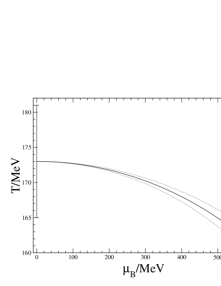
Figure 4.4: Left: The phase diagram obtained from the Taylor expansion method using two flavors of p4 improved fermions with a pion mass of $\approx$750 MeV (figure from Ref. [73]). Right: The phase diagram via analytic continuation from imaginary $\mu$ using two flavors of standard staggered fermions and a pion mass of $\approx$230 MeV [75].

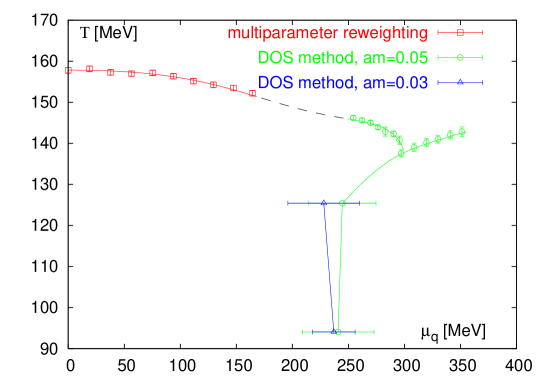
Figure 4.5: The phase diagram of four flavour staggered QCD obtained with the density of states method on $N_{t}=4$ lattices. A triple point was found at around 300 MeV quark chemical potential [86].

4.4.2 The critical point

One of the most important features of the phase diagram is the possible critical point separating a crossover region from a first-order phase transition regime. If such a point exists, its location is an unambiguous prediction of QCD.

Since real phase transitions only occur at infinite volume a determination of the order of the transition and thus locating the critical point is only possible via a finite size scaling analysis. At a single, finite volume everything is analytic, no real phase transitions –and thus no critical point– exist.

There are different possible strategies to locate the critical point. One can use Lee-Yang zeroes, Binder-cumulants or the convergence radius of the free energy density. These techniques will be discussed below. They can be applied directly, by determining the appropriate observables at finite $\mu$ using one of the methods described before. Another possibility is to start from a non-physical point (using small quark masses) where the critical point is located at zero or purely imaginary $\mu$ values and then determine the quark mass dependence of the critical point and extrapolate to the physical quark masses. The extrapolation, as usual, introduces errors, which are difficult to control.

At finite volumes the transition between the hadronic and quark-gluon phases is always continuous, the free energy density is analytic for all real values of the parameters of the action. Nevertheless, the partition function has zeroes even for finite volumes at complex values of the parameters. For a first-order phase transition these zeroes approach the real axis when the volume is increased – thus generating the singularity of the free energy for real parameter values. A detailed analysis shows that the imaginary part of these Lee-Yang zeroes scales as $1/V$ for large volumes. For a crossover the Lee-Yang zeroes do not approach the real axis when the volume is increased. Therefore inspecting the volume dependence of the imaginary parts of the Lee-Yang zeroes one can distinguish a first-order transition from an analytic crossover.

Binder cumulants can also be used to locate critical points. In the infinite volume limit they converge to 1 in case of first order phase transitions and specific values (determined by the universality class) for second order phase transitions. For details see e.g. Ref. [87] where the critical point of three flavor QCD at $\mu=0$ was determined using this technique.

The convergence radius of the Taylor expansion of the free energy gives the distance from the expansion point to the nearest singularity. If all expansion coefficients are positive then the singularity is at a real value of the expansion parameter which can than only be the critical point. As discussed before, this can only happen at infinite volume. The expansion coefficients have to be extrapolated to infinite volume, one has to be ensured that they are all positive and then the convergence radius can be calculated from them. Since the last two steps would require the knowledge of all coefficients (especially the positivity condition), this method gives a lower limit on the location of the critical point.

A necessary (but not satisfactory) condition of the existence of the critical point is a crossover at $\mu=0$. We have seen in the previous sections that using staggered fermions, this is indeed the case.

The multi-parameter reweighting combined with the Lee-Yang-zero analysis was used to locate the critical point. The first study was done with semi-realistic quark masses corresponding to a pion mass of $\approx$230 MeV [80]. The critical point was found at $T_{E}=160\pm 3.5$ MeV and $\mu_{E}=725\pm 35$ MeV. The whole study was repeated using larger volumes and physical quark masses in Ref. [83]. The results can be seen on Figure 4.6. The critical point is located at $T_{E}=162\pm 2$ MeV and $\mu_{E}=360\pm 40$ MeV. One can see that the critical point moved to a smaller value of $\mu$ as the quark masses were decreased. This is in complete agreement with expectations. It is important to emphasize again that both of these results were obtained for one set of lattice spacings, the continuum extrapolation is still missing.

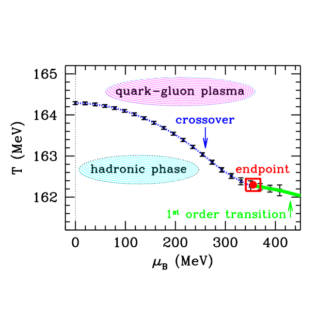
Figure 4.6: The phase diagram obtained with multi-parameter reweighting using 2+1 flavors of standard staggered fermions corresponding to the physical pion mass. The dotted part of the transition line is the crossover region while the solid line is of first order. The box shows the critical endpoint separating them.

The Taylor-expansion technique was used to determine the mass dependence of the critical point as discussed above. Starting from the three-flavor critical point where the phase transition is of second order at $\mu=0$, the derivative $d\mu_{E}/dm$ was determined. A linear extrapolation to larger quark masses using only this first derivative gave $\mu_{E}\approx 420$ MeV for the location of the critical point for physical quark masses [88]. Although an extrapolation to very distant quark masses was done which introduces unknown and possibly large errors, this value is in agreement with the value obtained directly via multi-parameter reweighting.

Another application of the Taylor-expansion method was done in Ref. [89] using two flavors of staggered fermions. The convergence radius of the series was estimated using the first few coefficients. The authors found $T_{E}\approx 0.95T_{c}$ and $\mu_{E}\approx 1.1T_{E}$ which is significantly smaller than the multi-parameter reweighting result. We should not forget, however, that –as discussed before– this result can only be considered as a lower limit on the location of the critical point.

For small enough quark masses the critical point can be located at a purely imaginary $\mu$. Approaching the point where the critical point reaches $\mu=0$ one can determine the derivative $d\mu_{E}^{2}/dm$ for negative values of $\mu_{E}^{2}$. This analysis was carried out in Refs. [90, 91]. For negative values of $\mu^{2}$ the critical quark mass $m_{c}$ was located and the derivative $dm_{c}/d\mu^{2}$ was determined (which is just the inverse of the above quoted derivative).

In Ref. [90] $dm_{c}/d\mu^{2}$ was found rather small which by a rough, linear extrapolation would suggest a much larger value of $\mu_{E}$ for physical quark masses than found e.g. by multi-parameter reweighting. More interestingly, when a similar analysis was done using an exact simulation algorithm instead of the previously applied approximate R algorithm, $dm_{c}/d\mu^{2}$ was found to be negative (but consistent with zero on the two-$\sigma$ level) [91]. Further calculations increased the significanse of this result greatly [92]. However, both calculations were done on coarse, $N_{t}=4$ lattices only. Conventionally, a positive value is expected for the derivative which was also observed with multi-parameter reweighting (larger quark masses lead to a larger value of $\mu_{E}$). Effective model calculations also support the positive sign (for a recent study, see e.g. [93]). Future lattice studies on finer lattices, and eventually a continuum extrapolation will give the final answer.

4.5 Equation of state at $\mu>0$

Besides the transition line and the critical point one can also determine the equation of state above and slightly below the transition line. The pressure can be calculated similarly to the $\mu=0$ case using the integral method. The only difference is that now we also have to include the chemical potential as an integration variable:

$$\frac{p}{T^{4}}=N_{t}^{4}\int^{(\beta,am_{q},a\mu)}_{(\beta_{0},am_{q0},a\mu_{0})}d(\beta,am_{q},a\mu)\left[\frac{1}{N_{t}N_{s}^{3}}\left(\begin{array}[]{c}{\partial\ln Z}/{\partial\beta}\\ {\partial\ln Z}/{\partial(am_{q})}\\ {\partial\ln Z}/{\partial(a\mu)}\\ \end{array}\right)\right.-$$ (4.19)

$$\left.\frac{1}{N_{t0}N_{s0}^{3}}\left(\begin{array}[]{c}{\partial\ln Z_{0}}/{\partial\beta}\\ {\partial\ln Z_{0}}/{\partial(am_{q})}\\ {\partial\ln Z_{0}}/{\partial(a\mu)}\end{array}\right)\right].$$ (4.23)

This expression is analogous to the one applied at $\mu=0$. The partial derivatives of $\ln Z$ correspond to the same observables as before. The only new one is ${\partial\ln Z_{0}}/{\partial(a\mu)}$ which is proportional to the $n_{q}$ quark number density. To carry out the integration one has to calculate the expectation values of these observables at non-vanishing $\mu$. This can be achieved by any of the previously discussed methods. In the following we discuss shortly the case of reweighting.

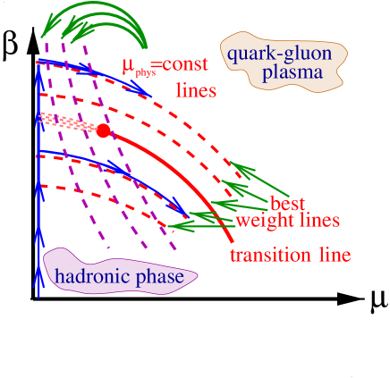
Figure 4.7: The contours used in the integral method to evaluate the pressure on the $\beta$–$\mu$ plane (blue lines). First, we integrate from $\mu=0$ up to some $\beta_{0}$ along the LCP. Then a best weight line is followed to the target $\beta,\mu$ values (red dashed lines).

Any observable can be evaluated at finite $\mu$ by reweighting (with or without Taylor expansion) using eqns. (4.3) and (4.4). In order to maximize the overlap between the configurations generated at $\mu=0$ and the target ensemble, one has to choose the starting point of the reweighting ($\beta_{0}$ at $\mu=0$) properly. One possibility is to minimize the spread of the weights of the configurations appearing in eqn. (4.4). This leads to the best weight lines, which are illustrated on Figure 4.7. The pressure can be calculated by following the lines indicated on the figure.

Since the pressure at small chemical potentials differs only slightly from the $\mu=0$ pressure, it is useful to define the difference as: $\Delta p=p(\mu)-p(\mu=0)$. Figure 4.8 shows the pressure for five chemical potentials obtained by multi-parameter reweighting [94, 95]. For this analysis standard staggered fermions were used on $N_{t}=4$ lattices. It is interesting that normalizing the shown curves by the Stephan-Boltzmann value at the given $\mu$-s, one gets an almost universal behaviour (see Figure 4.9).

The pressure difference has also been determined by the Bielefeld-Swansea collaboration [96, 97]. Their result is shown on Figure 4.10. It was obtained with p4 staggered fermions on $N_{t}=4$ lattices [96]. Since no continuum limit was taken in either case, the results do not have to be in completely consistent. Nevertheless they seem to show a nice qualitative agreement.

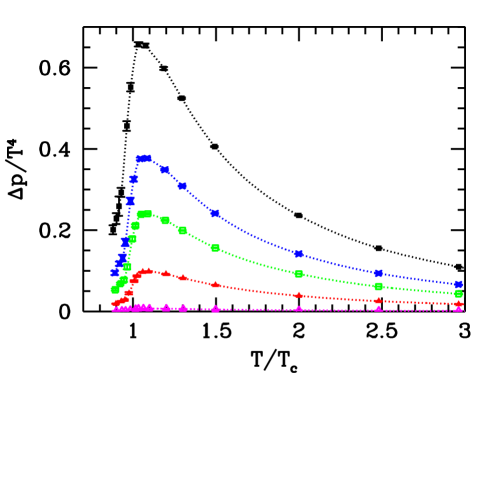
Figure 4.8: The $\Delta p$ pressure difference for several baryonic chemical potentials. The curves (from bottom to top) correspond to $\mu_{B}=$100, 210, 330, 410 and 530 MeV.

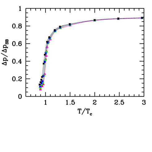
Figure 4.9: The $\Delta p$ pressure difference normalized by the Stefan-Boltzmann limit for different baryonic chemical potentials. The curves correspond to $\mu_{B}=$100 (purple), 210 (red), 330 (green), 410 (blue) and 530 MeV (black). They all seem to show a universal $\mu$ independent behavior.

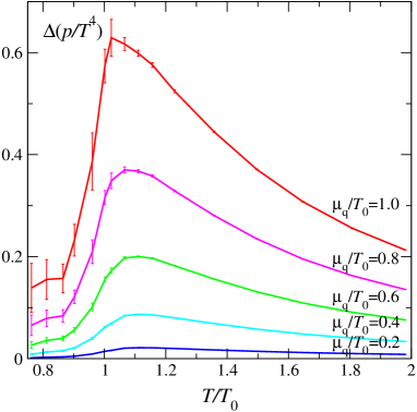
Figure 4.10: The $\Delta p$ pressure difference calculated by the Bielefeld-Swansea collaboration [96] for five different $\mu$ values. The quark chemical potential, normalized by the transition temperature $T_{0}$ ranges from 0.2 to 1.

5 Conclusions, outlook

A lattice result can be considered as a full result if two conditions are fulfilled. The first condition is related to the quark masses. We need results for physical quark masses, or in other words $m_{\pi}$$\approx$135 MeV and $m_{K}$$\approx$500 MeV. Controlled extrapolation in the quark masses around the transition temperature are not easy. Note, however, that today computers are quite often capable to deal with physical or almost physical quark masses. The second condition is the continuum extrapolation. It can be reached only by measuring quantities at non-vanishing lattice spacings and then extrapolating to vanishing lattice spacings. Luckily enough the choice of the action tells us what sort of functional form of the lattice spacings we expect for the deviation from the continuum limit result. If this asymptotic behavior is already present, we are in the so-called scaling region. E.g. for small enough lattice spacings results obtained by the standard Wilson action deviate from the continuum result by a linear term in the lattice spacing; for the staggered formalism this dependence is quadratic in the lattice spacings. Clearly, one should have an evidence that the results are already in this scaling region, which is described by the asymptotic lattice spacing dependence. For this check results at several lattice spacings are needed. Note, that thermodynamic studies are carried out on lattices, which have smaller temporal than spatial extensions. Typically one uses $N_{t}$=4,6,8 and 10, which –as a rule of thumb– correspond to lattice spacings: $\approx$0.3, 0.2, 0.15 and 0.12 fm, respectively (particularly at small $N_{t}$ values, the lattice spacing in physical unit is quite ambiguous, different physical quantities give different results, this ambiguity disappears when we approach the continuum limit).

Let us summarize what is known about our specific question, about the phase diagram of QCD. In some cases the result can be considered as a full one (at least using one specific formalism e.g. staggered one). In other cases one can estimate that the full result can be obtained in a year or two. There are however questions, which need much more time to clarify, particularly the controlled continuum limit is a difficult task.

a.) At vanishing chemical chemical potential the nature of the T$\neq$0 QCD transition is an analytic crossover [34]. The result was obtained with physical quark masses in the staggered formalism. This result can be considered as the full one. (As for any result of such type and huge complexity at least one independent analysis of the same depths is required to exclude any mistakes.) There are two, though unlikely possible uncertainties of this finding. One of them is a question, what happens if 2+1 flavor staggered QCD happens to be not in the QCD universality class. Though we do not have any theoretical proof for this universality class question, there is no sign for such a problematic scenario. Staggered lattice results for the whole spectrum and decay rates are in complete agreement with the experiments. Nevertheless it would be important to repeat the calculation with other fermion formulations (e.g. with Wilson fermions). This can be done with computer resources which are about an order of magnitude larger than the presently available ones. Since the rapid crossover is a remnant of the chiral transition of the massless theory, it would be very interesting to study the question what happens in the chiral limit. This question needs the same symmetry on the lattice as in the continuum theory. The best choice is the overlap fermion. Calculations with overlap fermions are usually two orders of magnitude more CPU-demanding than calculations with Wilson fermions. The other inconvenient possibility is related to the continuum extrapolation. It is possible –though quite unlikely– that after observing a consistent and finite continuum limit for the chiral susceptibility a completely different (phase transition-like, therefore divergent) continuum limit appears at even smaller lattice spacings. Note, that the transition turned out to be weaker and weaker as one decreased the lattice spacings. Thus, the above scenario –real phase transition in the continuum limit– would mean a completely opposite lattice spacing dependence as it was observed. This is the main reason, why one considers this possibility quite unlikely. In order to go to even smaller lattice spacings (e.g. $N_{t}$=12 or 14) approximately 1–2 orders of magnitude more CPU capacity is needed.

b.) We know the starting point of the phase diagram, namely the transition temperature of the crossover at vanishing chemical potential. Since the transition is an analytic one, there is no unique transition temperature. Different observables lead to different transition temperatures. According to Ref. [55] the width of the transition can be as large as $\approx$40 MeV. Thus, transition temperatures, depending on the definition, can be typically between $\approx$150 and 190 MeV. The actual values are still debated. E.g. for the peak in the $\chi/T^{2}$ distribution ($\chi$ is the unrenormalized chiral susceptibility) Ref. [33] used two different lattice spacings, namely $N_{t}$=4 and 6, and obtained 192 MeV. For the peak in the $\chi_{r}/T^{4}$ distribution ($\chi_{r}$ is the renormalized chiral susceptibility) Ref. [55] used also finer lattices with four different lattice spacings, namely $N_{t}$=4,6,8 and 10, and obtained 151 MeV (note, that for $\chi_{r}/T^{2}$ the obtained value is about 10 MeV higher). It is worth mentioning that for Ref. [55] the transition temperature is independent of the choice of the overall scale, whereas Ref. [33] is still in the scaling violation region (for their large lattice spacings the ratios of physical quantities are several sigma away from their experimental values). Since the available CPU-capacity is enough to carry out independent lattice simulations on $N_{t}$=8 and perhaps even on $N_{t}$=10 lattices, this controversy will be resolved in a year or two. The two possible but unlikely uncertainties, mentioned in the previous paragraph, are relevant also for the transition temperature. Therefore, one should determine the $\mu$=0 transition temperature using other formulations of lattice QCD (e.g. Wilson fermions or chiral fermions), and double check the results with even smaller lattice spacings.

c.) The curvature of the phase diagram at vanishing chemical potential is known at a$\approx$0.3 fm lattice spacings. Results were obtained by standard and p4 improved lattice actions for 2, 2+1 and 4 flavors [73, 75, 84, 83]. Though different choices of the QCD action should not necessarily give the same result at this rather large lattice spacing, results are in good agreement. If one takes the same action different techniques (multi-parameter reweighting with full determinant, Taylor expansion, analytic continuation) give the same result upto several digits. This nice agreement shows that the available methods are consistent. Clearly, the major drawback of these findings is the lack of the continuum extrapolation. Similarly to the determination of the crossover temperature the continuum extrapolation might change the a$\approx$0.3 fm results quite significantly. The available computer resources allow the determination of the curvature in the continuum limit in a year or two. It is important to emphasize again, that the staggered formalism has an unclarified uncertainty, therefore the whole calculation should be repeated in the Wilson formalism, too. Such a Wilson analysis is about an order of magnitude more CPU-demanding than the staggered one.

d.) There are several results for the existence and/or location of the critical point on the temperature versus chemical potential plane. All these results were obtained at quite large lattice spacings a$\approx$0.3 fm. We discussed in detail the difficulties and the problematic features of the available methods. Let us point out a more general difficulty, which is related to the continuum extrapolation. As one determines the nature of the transition at vanishing chemical potentials, it turns out that the transition gets weaker and weaker for smaller and smaller lattice spacings. This feature suggests, that the critical point, if it exists, might be at larger chemical potential in the continuum limit than on $N_{t}$=4 lattices. Unfortunately, for large chemical potentials the available methods are less reliable, which is particularly true for the staggered formalism (see Ref. [79] for a discussion on the staggered eigenvalue quartets, which suggests to use quite small lattice spacings). Searching for features at relatively large chemical potentials and at small lattice spacings is a very difficult and particularly CPU-demanding task. It is unlikely that the available methods with the present computer-resources can give a continuum extrapolated staggered result in a few years. The available methods are all applicable for Wilson fermions, too. On the one hand Wilson fermions do not have problems related to the rooting of the determinant (c.f. [79]), on the other hand the full diagonalization of the Wilson matrix is about two orders of magnitude more CPU-consuming. Furthermore, we do not have much experience how Wilson thermodynamics approaches the continuum limit, therefore it is hard to say what temporal extensions are needed to approach the continuum limit. The overlap formalism has all the symmetries of the theory even at non-vanishing lattice spacings, which is an advantage when we look for critical behavior. Though the available methods are applicable also for overlap fermions, the CPU-costs would be very large. To summarize: the presently available resources do not allow to extrapolate into the continuum limit. Results on the critical point at one or two non-vanishing lattice spacings can not be considered as full results.

e.) There is one exploratory lattice result on the triple point of QCD [86]. The lattice spacing is quite large, the volumes are small and four flavor is applied to avoid the rooting problem. This density of states method reached approximately three times larger chemical potentials than other methods in the literature. The CPU-costs (for this factor of three) were about two orders of magnitude larger than for the other methods. The method works, but it is clear that due to limited resources the continuum limit statement on the triple point can not be given in the near future.

Bibliography

- [1] J. Kuti, J. Polonyi, and K. Szlachanyi, Monte Carlo Study of SU(2) Gauge Theory at Finite Temperature, Phys. Lett. B98 (1981) 199.
- [2] L. D. McLerran and B. Svetitsky, A Monte Carlo Study of SU(2) Yang-Mills Theory at Finite Temperature, Phys. Lett. B98 (1981) 195.
- [3] T. Celik, J. Engels, and H. Satz, The Order of the Deconfinement Transition in SU(3) Yang- Mills Theory, Phys. Lett. B125 (1983) 411.
- [4] J. B. Kogut et al., Deconfinement and Chiral Symmetry Restoration at Finite Temperatures in SU(2) and SU(3) Gauge Theories, Phys. Rev. Lett. 50 (1983) 393.
- [5] S. A. Gottlieb et al., The Deconfining Phase Transition and the Continuum Limit of Lattice Quantum Chromodynamics, Phys. Rev. Lett. 55 (1985) 1958.
- [6] F. R. Brown, N. H. Christ, Y. F. Deng, M. S. Gao, and T. J. Woch, Nature of the Deconfining Phase Transition in SU(3) Lattice Gauge Theory, Phys. Rev. Lett. 61 (1988) 2058.
- [7] M. Fukugita, M. Okawa, and A. Ukawa, ORDER OF THE DECONFINING PHASE TRANSITION IN SU(3) LATTICE GAUGE THEORY, Phys. Rev. Lett. 63 (1989) 1768.
- [8] R. D. Pisarski and F. Wilczek, Remarks on the Chiral Phase Transition in Chromodynamics, Phys. Rev. D29 (1984) 338–341.
- [9] S. P. Klevansky, The Nambu-Jona-Lasinio model of quantum chromodynamics, Rev. Mod. Phys. 64 (1992) 649–708.
- [10] I. Montvay and G. Munster, Quantum fields on a lattice, . Cambridge, UK: Univ. Pr. (1994) 491 p. (Cambridge monographs on mathematical physics).
- [11] H. B. Nielsen and M. Ninomiya, Absence of Neutrinos on a Lattice. 1. Proof by Homotopy Theory, Nucl. Phys. B185 (1981) 20.
- [12] H. B. Nielsen and M. Ninomiya, Absence of Neutrinos on a Lattice. 2. Intuitive Topological Proof, Nucl. Phys. B193 (1981) 173.
- [13] H. Neuberger, Exactly massless quarks on the lattice, Phys. Lett. B417 (1998) 141–144, [hep-lat/9707022].
- [14] M. Luscher, Exact chiral symmetry on the lattice and the Ginsparg- Wilson relation, Phys. Lett. B428 (1998) 342–345, [hep-lat/9802011].
- [15] Z. Fodor, S. D. Katz, and K. K. Szabo, Dynamical overlap fermions, results with hybrid Monte- Carlo algorithm, JHEP 08 (2004) 003, [hep-lat/0311010].
- [16] N. Cundy, Dynmical overlap, . Prepared for 58th Scottish Universities Summer School in Physics (SUSSP58): A NATO Advanced Study Institute and EU Hadron Physics 13 Summer Institute, St. Andrews, Scotland, 22-29 Aug 2004.
- [17] T. A. DeGrand and S. Schaefer, Physics issues in simulations with dynamical overlap fermions, Phys. Rev. D71 (2005) 034507, [hep-lat/0412005].
- [18] G. I. Egri, Z. Fodor, S. D. Katz, and K. K. Szabo, Topology with dynamical overlap fermions, JHEP 01 (2006) 049, [hep-lat/0510117].
- [19] C. B. Lang, P. Majumdar, and W. Ortner, QCD with two dynamical flavors of chirally improved quarks, Phys. Rev. D73 (2006) 034507, [hep-lat/0512014].
- [20] JLQCD Collaboration, H. Fukaya et al., Lattice gauge action suppressing near-zero modes of H(W), Phys. Rev. D74 (2006) 094505, [hep-lat/0607020].
- [21] C. Bernard, M. Golterman, and Y. Shamir, Observations on staggered fermions at non-zero lattice spacing, Phys. Rev. D73 (2006) 114511, [hep-lat/0604017].
- [22] P. Hasenfratz and F. Niedermayer, Perfect lattice action for asymptotically free theories, Nucl. Phys. B414 (1994) 785–814, [hep-lat/9308004].
- [23] T. A. DeGrand, A. Hasenfratz, P. Hasenfratz, and F. Niedermayer, The Classically perfect fixed point action for SU(3) gauge theory, Nucl. Phys. B454 (1995) 587–614, [hep-lat/9506030].
- [24] J. Polonyi and H. W. Wyld, Microcanonical Simulation of Fermionic Systems, Phys. Rev. Lett. 51 (1983) 2257.
- [25] R. T. Scalettar, D. J. Scalapino, and R. L. Sugar, NEW ALGORITHM FOR THE NUMERICAL SIMULATION OF FERMIONS, Phys. Rev. B34 (1986) 7911–7917.
- [26] S. Duane, A. D. Kennedy, B. J. Pendleton, and D. Roweth, Hybrid Monte Carlo, Phys. Lett. B195 (1987) 216–222.
- [27] S. A. Gottlieb, W. Liu, D. Toussaint, R. L. Renken, and R. L. Sugar, Hybrid Molecular Dynamics Algorithms for the Numerical Simulation of Quantum Chromodynamics, Phys. Rev. D35 (1987) 2531–2542.
- [28] M. A. Clark and A. D. Kennedy, Accelerating Staggered Fermion Dynamics with the Rational Hybrid Monte Carlo (RHMC) Algorithm, Phys. Rev. D75 (2007) 011502, [hep-lat/0610047].
- [29] U. M. Heller, F. Karsch, and B. Sturm, Improved staggered fermion actions for QCD thermodynamics, Phys. Rev. D60 (1999) 114502, [hep-lat/9901010].
- [30] C. Morningstar and M. J. Peardon, Analytic smearing of SU(3) link variables in lattice QCD, Phys. Rev. D69 (2004) 054501, [hep-lat/0311018].
- [31] Y. Aoki, Z. Fodor, S. D. Katz, and K. K. Szabo, The equation of state in lattice QCD: With physical quark masses towards the continuum limit, JHEP 01 (2006) 089, [hep-lat/0510084].
- [32] C. Bernard et al., The equation of state for QCD with 2+1 flavors of quarks, PoS LAT2005 (2006) 156, [hep-lat/0509053].
- [33] M. Cheng et al., The transition temperature in QCD, Phys. Rev. D74 (2006) 054507, [hep-lat/0608013].
- [34] Y. Aoki, G. Endrodi, Z. Fodor, S. D. Katz, and K. K. Szabo, The order of the quantum chromodynamics transition predicted by the standard model of particle physics, Nature 443 (2006) 675–678, [hep-lat/0611014].
- [35] R. Sommer, A New way to set the energy scale in lattice gauge theories and its applications to the static force and alpha-s in SU(2) Yang-Mills theory, Nucl. Phys. B411 (1994) 839–854, [hep-lat/9310022].
- [36] C. Aubin et al., Light hadrons with improved staggered quarks: Approaching the continuum limit, Phys. Rev. D70 (2004) 094505, [hep-lat/0402030].
- [37] A. Gray et al., The Upsilon spectrum and m(b) from full lattice QCD, Phys. Rev. D72 (2005) 094507, [hep-lat/0507013].
- [38] European Twisted Mass Collaboration, C. Alexandrou et al., Light baryon masses with dynamical twisted mass fermions, Phys. Rev. D78 (2008) 014509, [0803.3190].
- [39] M. Gockeler et al., A determination of the Lambda parameter from full lattice QCD, Phys. Rev. D73 (2006) 014513, [hep-ph/0502212].
- [40] PACS-CS Collaboration, S. Aoki et al., 2+1 Flavor Lattice QCD toward the Physical Point, 0807.1661.
- [41] Particle Data Group Collaboration, C. Amsler et al., Review of particle physics, Phys. Lett. B667 (2008) 1.
- [42] D. J. Schwarz, The first second of the universe, Annalen Phys. 12 (2003) 220–270, [astro-ph/0303574].
- [43] E. Witten, Cosmic Separation of Phases, Phys. Rev. D30 (1984) 272–285.
- [44] J. H. Applegate and C. J. Hogan, Relics of Cosmic Quark Condensation, Phys. Rev. D31 (1985) 3037–3045.
- [45] A. M. Halasz, A. D. Jackson, R. E. Shrock, M. A. Stephanov, and J. J. M. Verbaarschot, On the phase diagram of QCD, Phys. Rev. D58 (1998) 096007, [hep-ph/9804290].
- [46] J. Berges and K. Rajagopal, Color superconductivity and chiral symmetry restoration at nonzero baryon density and temperature, Nucl. Phys. B538 (1999) 215–232, [hep-ph/9804233].
- [47] B.-J. Schaefer and J. Wambach, The phase diagram of the quark meson model, Nucl. Phys. A757 (2005) 479–492, [nucl-th/0403039].
- [48] T. Herpay, A. Patkos, Z. Szep, and P. Szepfalusy, Mapping the boundary of the first order finite temperature restoration of chiral symmetry in the (m(pi) - m(K))-plane with a linear sigma model, Phys. Rev. D71 (2005) 125017, [hep-ph/0504167].
- [49] F. Karsch et al., Where is the chiral critical point in 3-flavor QCD?, Nucl. Phys. Proc. Suppl. 129 (2004) 614–616, [hep-lat/0309116].
- [50] P. de Forcrand, S. Kim, and O. Philipsen, A QCD chiral critical point at small chemical potential: is it there or not?, PoS LAT2007 (2007) 178, [0711.0262].
- [51] G. Endrodi, Z. Fodor, S. D. Katz, and K. K. Szabo, The nature of the finite temperature QCD transition as a function of the quark masses, PoS LAT2007 (2007) 182, [0710.0998].
- [52] MILC Collaboration, C. Bernard et al., QCD thermodynamics with three flavors of improved staggered quarks, Phys. Rev. D71 (2005) 034504, [hep-lat/0405029].
- [53] O. Kaczmarek, F. Karsch, P. Petreczky, and F. Zantow, Heavy quark anti-quark free energy and the renormalized Polyakov loop, Phys. Lett. B543 (2002) 41–47, [hep-lat/0207002].
- [54] Z. Fodor, S. D. Katz, K. K. Szabo, and A. I. Toth, Grand canonical potential for a static quark anti-quark pair at mu not equal 0, Nucl. Phys. Proc. Suppl. 140 (2005) 508–510, [hep-lat/0410032].
- [55] Y. Aoki, Z. Fodor, S. D. Katz, and K. K. Szabo, The QCD transition temperature: Results with physical masses in the continuum limit, Phys. Lett. B643 (2006) 46–54, [hep-lat/0609068].
- [56] G. Boyd et al., Thermodynamics of SU(3) Lattice Gauge Theory, Nucl. Phys. B469 (1996) 419–444, [hep-lat/9602007].
- [57] CP-PACS Collaboration, M. Okamoto et al., Equation of state for pure SU(3) gauge theory with renormalization group improved action, Phys. Rev. D60 (1999) 094510, [hep-lat/9905005].
- [58] CP-PACS Collaboration, Y. Namekawa et al., Thermodynamics of SU(3) gauge theory on anisotropic lattices, Phys. Rev. D64 (2001) 074507, [hep-lat/0105012].
- [59] G. Endrodi, Z. Fodor, S. D. Katz, and K. K. Szabo, The equation of state at high temperatures from lattice QCD, PoS LAT2007 (2007) 228, [0710.4197].
- [60] T. Blum, L. Karkkainen, D. Toussaint, and S. A. Gottlieb, The beta function and equation of state for QCD with two flavors of quarks, Phys. Rev. D51 (1995) 5153–5164, [hep-lat/9410014].
- [61] MILC Collaboration, C. W. Bernard et al., The equation of state for two flavor QCD at N(t) = 6, Phys. Rev. D55 (1997) 6861–6869, [hep-lat/9612025].
- [62] F. Karsch, E. Laermann, and A. Peikert, The pressure in 2, 2+1 and 3 flavour QCD, Phys. Lett. B478 (2000) 447–455, [hep-lat/0002003].
- [63] M. Cheng et al., The QCD Equation of State with almost Physical Quark Masses, Phys. Rev. D77 (2008) 014511, [0710.0354].
- [64] C. Bernard et al., QCD equation of state with 2+1 flavors of improved staggered quarks, Phys. Rev. D75 (2007) 094505, [hep-lat/0611031].
- [65] J. Engels, J. Fingberg, F. Karsch, D. Miller, and M. Weber, Nonperturbative thermodynamics of SU(N) gauge theories, Phys. Lett. B252 (1990) 625–630.
- [66] Y. Aoki et al., The QCD transition temperature: results with physical masses in the continuum limit II, JHEP 06 (2009) 088, [0903.4155].
- [67] A. Bazavov et al., Equation of state and QCD transition at finite temperature, Phys. Rev. D80 (2009) 014504, [0903.4379].
- [68] RBC Collaboration, F. Karsch, Equation of state and more from lattice regularized QCD, J. Phys. G35 (2008) 104096, [0804.4148].
- [69] F. Karsch, Recent lattice results on finite temperature and density QCD, part I, PoS CPOD07 (2007) 026, [0711.0656].
- [70] I. M. Barbour, S. E. Morrison, E. G. Klepfish, J. B. Kogut, and M.-P. Lombardo, Results on finite density QCD, Nucl. Phys. Proc. Suppl. 60A (1998) 220–234, [hep-lat/9705042].
- [71] P. Hasenfratz and F. Karsch, Chemical Potential on the Lattice, Phys. Lett. B125 (1983) 308.
- [72] Z. Fodor and S. D. Katz, A new method to study lattice QCD at finite temperature and chemical potential, Phys. Lett. B534 (2002) 87–92, [hep-lat/0104001].
- [73] C. R. Allton et al., The QCD thermal phase transition in the presence of a small chemical potential, Phys. Rev. D66 (2002) 074507, [hep-lat/0204010].
- [74] P. de Forcrand, S. Kim, and T. Takaishi, Qcd simulations at small chemical potential, Nucl. Phys. Proc. Suppl. 119 (2003) 541–543, [hep-lat/0209126].
- [75] P. de Forcrand and O. Philipsen, The qcd phase diagram for small densities from imaginary chemical potential, Nucl. Phys. B642 (2002) 290–306, [hep-lat/0205016].
- [76] V. Azcoiti, G. Di Carlo, A. Galante, and V. Laliena, Finite density QCD: A new approach, JHEP 12 (2004) 010, [hep-lat/0409157].
- [77] S. Kratochvila and P. de Forcrand, QCD at small baryon number, Nucl. Phys. Proc. Suppl. 140 (2005) 514–516, [hep-lat/0409072].
- [78] A. Alexandru, M. Faber, I. Horvath, and K.-F. Liu, Lattice QCD at finite density via a new canonical approach, Phys. Rev. D72 (2005) 114513, [hep-lat/0507020].
- [79] M. Golterman, Y. Shamir, and B. Svetitsky, Breakdown of staggered fermions at nonzero chemical potential, Phys. Rev. D74 (2006) 071501, [hep-lat/0602026].
- [80] Z. Fodor and S. D. Katz, Lattice determination of the critical point of QCD at finite T and mu, JHEP 03 (2002) 014, [hep-lat/0106002].
- [81] C.-N. Yang and T. D. Lee, Statistical theory of equations of state and phase transitions. I: Theory of condensation, Phys. Rev. 87 (1952) 404–409.
- [82] T. D. Lee and C.-N. Yang, Statistical theory of equations of state and phase transitions. II: Lattice gas and Ising model, Phys. Rev. 87 (1952) 410–419.
- [83] Z. Fodor and S. D. Katz, Critical point of QCD at finite T and mu, lattice results for physical quark masses, JHEP 04 (2004) 050, [hep-lat/0402006].
- [84] M. D’Elia and M.-P. Lombardo, Finite density qcd via imaginary chemical potential, Phys. Rev. D67 (2003) 014505, [hep-lat/0209146].
- [85] V. Azcoiti, G. Di Carlo, A. Galante, and V. Laliena, Phase diagram of QCD with four quark flavors at finite temperature and baryon density, Nucl. Phys. B723 (2005) 77–90, [hep-lat/0503010].
- [86] Z. Fodor, S. D. Katz, and C. Schmidt, The density of states method at non-zero chemical potential, JHEP 03 (2007) 121, [hep-lat/0701022].
- [87] F. Karsch, E. Laermann, and C. Schmidt, The chiral critical point in 3-flavor QCD, Phys. Lett. B520 (2001) 41–49, [hep-lat/0107020].
- [88] S. Ejiri et al., Study of QCD thermodynamics at finite density by Taylor expansion, Prog. Theor. Phys. Suppl. 153 (2004) 118–126, [hep-lat/0312006].
- [89] R. V. Gavai and S. Gupta, The critical end point of QCD, Phys. Rev. D71 (2005) 114014, [hep-lat/0412035].
- [90] P. de Forcrand and O. Philipsen, The qcd phase diagram for three degenerate flavors and small baryon density, Nucl. Phys. B673 (2003) 170, [hep-lat/030702].
- [91] P. de Forcrand and O. Philipsen, The chiral critical line of N(f) = 2+1 QCD at zero and non-zero baryon density, JHEP 01 (2007) 077, [hep-lat/0607017].
- [92] P. de Forcrand and O. Philipsen, The chiral critical point of Nf=3 QCD at finite density to the order , 0808.1096.
- [93] P. Kovacs and Z. Szep, The critical surface of the SU(3)L x SU(3)R chiral quark model at non-zero baryon density, Phys. Rev. D75 (2007) 025015, [hep-ph/0611208].
- [94] Z. Fodor, S. D. Katz, and K. K. Szabo, The QCD equation of state at nonzero densities: Lattice result, Phys. Lett. B568 (2003) 73–77, [hep-lat/0208078].
- [95] F. Csikor et al., Equation of state at finite temperature and chemical potential, lattice QCD results, JHEP 05 (2004) 046, [hep-lat/0401016].
- [96] C. R. Allton et al., The equation of state for two flavor QCD at non-zero chemical potential, Phys. Rev. D68 (2003) 014507, [hep-lat/0305007].
- [97] C. R. Allton et al., Thermodynamics of two flavor QCD to sixth order in quark chemical potential, Phys. Rev. D71 (2005) 054508, [hep-lat/0501030].