Regularized Reconstruction of MR Images from Spiral Acquisitions

Abstract

Combining fast MR acquisition sequences and high resolution imaging is a major issue in dynamic imaging. Reducing the acquisition time can be achieved by using non-Cartesian and sparse acquisitions. The reconstruction of MR images from these measurements is generally carried out using gridding that interpolates the missing data to obtain a dense Cartesian $k$-space filling. The MR image is then reconstructed using a conventional Fast Fourier Transform (FFT). The estimation of the missing data unavoidably introduces artifacts in the image that remain difficult to quantify.

A general reconstruction method is proposed to take into account these limitations. It can be applied to any sampling trajectory in $k$-space, Cartesian or not, and specifically takes into account the exact location of the measured data, without making any interpolation of the missing data in $k$-space. Information about the expected characteristics of the imaged object is introduced to preserve the spatial resolution and improve the signal to noise ratio in a regularization framework. The reconstructed image is obtained by minimizing a non-quadratic convex objective function. An original rewriting of this criterion is shown to strongly improve the reconstruction efficiency. Results on simulated data and on a real spiral acquisition are presented and discussed.

1 Introduction

In Magnetic Resonance Imaging (MRI) the acquired data are samples of the Fourier transform of the imaged object [1]. Acquisition is often discussed in terms of location in $k$-space and most conventional methods collect data on a regular Cartesian grid. This allows for a straightforward characterization of aliasing and Gibbs artifacts, and permits direct image reconstruction by means of 2D-Fast Fourier Transform (FFT) algorithms. Other acquisition sequences, such as spiral [2], PROPELLER [3], projection reconstruction, i.e. radial [4], rosette [5], collect data on a non-Cartesian grid. They possess many desirable properties, including reduction of the acquisition time and of various motion artifacts. The gridding procedure associated to an FFT is the most common method for Cartesian image reconstruction from such irregular $k$-space acquisitions.

Re-gridding data from non-Cartesian locations to a Cartesian grid has been addressed by many authors. O’Sullivan [6] introduced a convolution-interpolation technique in computerized tomography (CT) which can be applied to magnetic resonance imaging [2]. He suggested not to use a direct reconstruction, but to perform a convolution-interpolation of the data sampled on a polar pattern onto a Cartesian $k$-space. The final image was obtained by FFT. The stressed advantage of this technique was the reduction of computational complexity compared to the filtered back-projection technique. Moreover, it can be applied to any arbitrary trajectory in $k$-space.

More generally, the reconstruction process is four steps:

1. data weighting for nonuniform sampling compensation,

2. re-sampling onto a Cartesian grid, using a given kernel,

3. computation of the FFT,

4. correction for the kernel apodization.

Jackson et al. [7] precisely discussed criteria to choose an appropriate convolution kernel. This is necessary for accurate interpolation and also for minimization of reconstruction errors due to uneven weighting of $k$-space. Several authors have suggested methods for calculating this sampling density. Numerical solutions have been proposed that iteratively calculate the compensation weights [3]. But, for arbitrary trajectories, the weighting function is not known analytically and must somehow be extracted from the sampling function itself. A possible solution is to use the area of the Voronoi cell around each sample [8].

The gridding method is computationally efficient. However, convolution-interpolation methods unavoidably introduce artifacts in the reconstructed images [8]. Indeed, for a given kernel the convolution modifies data in $k$-space and it is difficult to know the exact effect of gridding in the image domain. Moreover, this method tends to correlate the noise in the measured samples and lacks solid analysis and design tools to quantify or minimize the reconstruction errors.

The principle of regularized reconstruction has been described by several authors for parallel imaging: [9], [10] and more recently [11] proposed the use of a general reconstruction method for sensitivity encoding (SENSE) [12] which has been applied with a quadratic regularization term and a Cartesian acquisition scheme. In this paper, we extend this work by: 1) giving a more general formulation of the reconstruction term for Non Cartesian trajectories, 2) specifically using the exact non-uniform locations of the acquired data in $k$-space, without the need for gridding the data to a uniform Cartesian grid and, 3) incorporate a non–quadratic convex regularization term in order to maintain edge sharpness compared to a purely quadratic term. The regularization term represents the prior information about the imaged object that improves the signal to noise ratio (SNR) of the reconstructed image as well as the spatial resolution.

In section 2, we recall the basis of MRI signal acquisition and the modelling of the MR acquisition process. Then we address the image reconstruction methods for different acquisition schemes and develop the proposed method, in section 3. The reconstruction is based on the iterative optimization of a Discrete Fourier Transform (DFT) regularized criterion. Rewriting this criterion allows to reduce the complexity of the computation and to decrease the reconstruction time. Finally, section 4 compares the proposed method and the gridding reconstruction for simulated and real sparse data acquired along interleaved spiral trajectories.

2 Direct model

MRI theory [1] indicates that the acquired signal $s$ is related to the imaged object $f$ through:

$$s({\mathb{k}}(t))=\iint_{D}f({\mathb{r}})\,{\mathrm{e}}^{i2\pi{\mathb{k}}(t)^{\mathrm{t}}{\mathb{r}}}\,{\mathrm{d}}{\mathb{r}}\,,$$ (1)

in a 2D context. $D$ is the field of view, i.e., the extent of the imaged object, ${\mathb{r}}$ is the spatial vector and ${\mathb{k}}(t)=[k_{x}(t),k_{y}(t)]^{\mathrm{t}}$ (“t” denotes a transpose) is the $k$-space trajectory. Thus, the received signal can be thought as the Fourier transform of the object, along a trajectory ${\mathb{k}}(t)$ determined by the magnetic gradient field ${\mathb{G}}(t)=[G_{x}(t),G_{y}(t)]^{\mathrm{t}}$:

$${\mathb{k}}(t)=\gamma\int_{0}^{t}{\mathb{G}}(t^{\prime})\,{\mathrm{d}}t^{\prime}.$$

The modulus of $f({\mathb{r}})$ is proportional to the spin density function and the phase factor is influenced by spin motions and magnetic field inhomogeneities.

Remark 1

— Eq. (1) presents a model for an ideal signal. Actual signals also include terms for the relaxation of the magnetic moments which will cause the signal amplitude to decrease, as well as a term for inhomogeneity within the image. By the way, they could be easily incorporated in (1), but for our purposes here we will ignore these effects.

Practically, the acquired signal is not a continuous function of time but made of a finite number of samples. This introduces the discretization of the data, and the measured data set writes ${\mathb{s}}=[s_{0},s_{1},\ldots,s_{L-1}]^{\mathrm{t}}\in{\mathbbm{C}}^{L}$, i.e., consists of $L$ data sampled along the discrete trajectory $[{\mathb{k}}_{0},{\mathb{k}}_{1},\ldots,{\mathb{k}}_{L-1}]$, where ${\mathb{k}}_{l}=[k_{x}^{l},k_{y}^{l}]^{\mathrm{t}}$. For a single sample, Eq. (1) then reads:

$$s_{l}=\iint_{D}f({\mathb{r}})\,{\mathrm{e}}^{i2\pi{\mathb{k}}_{l}^{\mathrm{t}}{\mathb{r}}}\,{\mathrm{d}}{\mathb{r}}\,.$$

Generally the object $f$ is not reconstructed as a continuous function of the spatial variables ${\mathb{r}}$ but is also discretized for practical considerations: to use image visualization and also to perform fast reconstruction techniques by means of FFT. This introduces a discretization of the unknown object and a common choice is a Cartesian grid of size $N\times N$. We note $f_{n,m}$ the unknown discretized object evaluated at locations ${\mathb{r}}_{nm}=[n,m]^{\mathrm{t}}$ with $n,m=0,1,\ldots,N-1$.

The discrete model is then given by an approximation of the integral of Eq. (1):

$$s_{l}=\frac{1}{N}\sum_{n,m=0}^{N-1}f_{n,m}\,{\mathrm{e}}^{i2\pi\left(k_{x}^{l}m/F_{x}+k_{y}^{l}n/F_{y}\right)}$$

where ${\mathb{F}}=[F_{x},F_{y}]^{\mathrm{t}}$ is the spatial sampling frequency of the object. To comply with the Shannon sampling frequency, ${\mathb{F}}$ must be chosen such as $F_{x}\geq 2/D_{x}$ and $F_{y}\geq 2/D_{y}$, where $D_{x}$ and $D_{y}$ are the dimensions of the field of view. For sake of simplicity we assume here that ${\mathb{F}}=[1,1]^{\mathrm{t}}$ and the spatial frequencies $k_{x}^{l}$ and $k_{y}^{l}$ are normalized and lie in $[-0.5,+0.5]$.

In practice the acquired samples are corrupted by a complex valued noise, denoted ${\mathb{b}}=[b_{0},\ldots,b_{L-1}]^{\mathrm{t}}\in{\mathbbm{C}}^{L}$, which can be assumed to be additive white and Gaussian [13].

We can then write, for one datum, the final discretized model as:

$$s_{l}=\frac{1}{N}\sum_{n,m=0}^{N-1}f_{n,m}\,{\mathrm{e}}^{i2\pi(k_{x}^{l}m+k_{y}^{l}n)}+b_{l}$$ (2)

for $l=0,\ldots,L-1$ or, more simply as

$$s_{l}={\mathb{h}}_{l}{\mathb{f}}+b_{l}\,,$$

with ${\mathb{f}}$ being a column vector, collecting the $f_{n,m}$ rearranged column by column in one vector, and ${\mathb{h}}_{l}$ a row vector

$${\mathb{h}}_{l}=\frac{1}{N}\,[{\mathrm{e}}^{i2\pi{\mathb{k}}_{l}^{\mathrm{t}}{\mathb{r}}_{00}},{\mathrm{e}}^{i2\pi{\mathb{k}}_{l}^{\mathrm{t}}{\mathb{r}}_{01}},\ldots,{\mathrm{e}}^{i2\pi{\mathb{k}}_{l}^{\mathrm{t}}{\mathb{r}}_{N-1,N-1}}]\,.$$

The whole data vector then writes:

$${\mathb{s}}=H{\mathb{f}}+{\mathb{b}},$$ (3)

where $H$ is the inverse Fourier matrix:

$$H=\left(\begin{array}[]{c}{\mathb{h}}_{0}\\ \hline\cr{\mathb{h}}_{1}\\ \hline\cr\vdots\\ \hline\cr{\mathb{h}}_{L-1}\\ \end{array}\right)\,,$$

depending on the acquisition locations.

Eq. (3) is a linear model with additive Gaussian noise. It has been extensively studied in literature [14]. The aim of the reconstruction process is to compute an estimate $\widehat{{\mathb{f}}}$ of the unknown object ${\mathb{f}}$ from the discrete, incomplete and noisy $k$-space samples ${\mathb{s}}$. The problem is referred to as a Fourier synthesis problem and consists of inversion of the model (3).

3 Model inversion

A usual inversion method relies on a Least Squares (LS) criterion, based on Eq. (3):

$${\mathcal{J}}_{\mathrm{\scriptscriptstyle LS}}({\mathb{f}})=||{\mathb{s}}-H{\mathb{f}}||^{2}=\sum_{l=0}^{L-1}|s_{l}-{\mathb{h}}_{l}{\mathb{f}}|^{2}\,.$$ (4)

The reconstructed image is the minimizer of ${\mathcal{J}}_{\mathrm{\scriptscriptstyle LS}}$:

$$\widehat{{\mathb{f}}}_{\mathrm{\scriptscriptstyle LS}}=\mathop{\mathrm{arg\,min}}_{{\mathb{f}}}{\mathcal{J}}_{\mathrm{\scriptscriptstyle LS}}({\mathb{f}})\,,$$

and minimizes the quadratic error between the measured data and the estimated ones generated by the direct model (3). The solution writes:

$$\widehat{{\mathb{f}}}_{\mathrm{\scriptscriptstyle LS}}=(H^{\dagger}H)^{-1}H^{\dagger}{\mathb{s}}\,,$$

if $H^{\dagger}H$ is invertible, property that depends on the acquisition scheme.

3.1 Cartesian and complete acquisitions

In Complete Cartesian (CC) acquisitions $H$ is the $N\times N$ inverse Fourier transform matrix, evaluated on an uniform grid. We then have $H^{\dagger}H=I$ and the LS solution simplifies to

$$\widehat{f}=H^{\dagger}{\mathb{s}}.$$ (5)

It is efficiently computed by the FFT of the raw data and the compromise between acquisition time and image characteristics depends only on the acquisition scheme.

This inversion method directly holds as long as a complete Cartesian $k$-space is available as for the conventional line by line acquisitions where one line is acquired for each successive radio-frequency (rf) excitation. It holds also for multi-shot acquisitions when more than a single $k$-space line is acquired for each rf excitation. It can finally be applied to EPI sequences when only one excitation is used to sample the whole $k$-space domain.

The method remains convenient for time segmented acquisitions that update only partially $k$-space, such as keyhole, BRISK or TRICKS techniques [15, 16, 17, 18] provided that a convenient filing of $k$-space data has been made previously.

3.2 Incomplete and non Cartesian acquisitions

Other acquisition schemes have been proposed in order to reduce acquisition time. They can be divided in two groups: Incomplete Cartesian (IC) ones and Non Cartesian (NC) ones.

1. Partial Cartesian filling of a $k$-space such as the widely used “half Fourier” method  [19] or variable density phase encoding technique [20] allow to reduce the number of acquired data and thus the acquisition time. In this case, $H$ is a partial matrix and can still be computed with the FFT.

2. Non Cartesian $k$-space filling (interleaved spirals, PROPELLER sequence, radial, concentric circles, rosettes…) conjugate a variable, non–uniform density encoding with specific gradient sequences with the same objective of acquisition time reduction. These acquisition schemes often require a small number of rf pulses, take advantage of the available gradient strength and rising time, reduce motion artifacts and lessen sensitivity to off-resonances and field inhomogeneities [2].

From a mathematical stand point, the main difficulty of the Non Cartesian acquisition schemes is that (5) cannot be computed using the FFT algorithm, since the samples are no longer on a uniform grid. Current strategies force the re-use of FFT reconstruction (5) by means of data pre-processing.

1. The missing data are completed beforehand using Fourier symmetry properties of the $k$-space [19] (see also the Margosian reconstruction [21]), or a zero-padding extrapolation. Conventional zero padding used to construct a square image from a rectangular acquisition matrix also belongs to this category.

2. The acquired data are interpolated and re-sampled by means of a gridding method.

Thus a complete Cartesian $k$-space is pre-computed from the acquired data and the final image is obtained by FFT. The wide availability of high-speed FFT routines and processors have made the method by far the most popular. But, such methods do not rely on the physical model (3) nor on the true acquired data: they introduce interpolated data resulting in inaccuracies in the reconstructed images. On the contrary, the proposed method accounts for exact locations of the data in $k$-space. The methodology is applicable for both IC and NC acquisition scheme and we concentrate on the NC case i.e. the non-uniform DFT model.

Other strategies rely on true DFT and LS framework. The main problem here is that $H^{\dagger}H$ is not invertible: the unknown image pixels usually outnumber the acquired data and the problem is indeterminate, i.e., ${\mathcal{J}}_{\mathrm{\scriptscriptstyle LS}}$ does not have a unique minimizer. From basic inverse problem theory, several regularization approaches have been proposed. Among the earliest are the Truncated Singular Value Decomposition (TSVD) and the Minimum Norm Least Squares (MNLS). They properly regularize the problem, alleviate the indeterminacy and define a solution to (3). The TSVD and the MNLS approaches have been proposed in MRI by [20] for IC acquisition and by [22, 23] for NC acquisitions, respectively. Practically they both can be extended for IC and NC acquisitions and behave similarly.

In any case (TSVD, MNLS, gridding, zero-padding), it is difficult to control the information accounted for, in order to regularize the problem. Moreover they cannot incorporate more specific information such as pixel correlation, and edge enhancement. The proposed method, described below, accounts for known common information about the expected images and exact locations of the data in the $k$-space.

3.3 Regularized Method

The proposed method relies on Regularized Least Squares (RLS) criterion:

$${\mathcal{J}}_{\mathrm{\scriptscriptstyle Reg}}({\mathb{f}})={\mathcal{J}}_{\mathrm{\scriptscriptstyle LS}}({\mathb{f}})+{\mathcal{R}}({\mathb{f}}).$$

It is based on the LS term and a prior one ${\mathcal{R}}$, that only depends upon the object ${\mathb{f}}$. The proposed solution writes:

$$\widehat{{\mathb{f}}}_{\mathrm{\scriptscriptstyle Reg}}=\mathop{\mathrm{arg\,min}}_{{\mathb{f}}}{\mathcal{J}}_{\mathrm{\scriptscriptstyle Reg}}({\mathb{f}})\,.$$

The choice of ${\mathcal{R}}$ depends on the information to be introduced. In MR, there are a great variety of image kinds, but at least two common characteristics are observed.

1. The structure have usually smooth variations and a good contrast compared to the surrounding organs, more particularly when contrast agents are used. These regions are separated by sharp transitions representing the edges.

2. The regions outside the imaged object i.e. the background is a region where ${\mathb{f}}$ is expected to be zero.

The proposed regularization term accounts for these information and takes the following form:

$${\mathcal{R}}({\mathb{f}})=\lambda_{1}\Omega_{1}({\mathb{f}})+\lambda_{0}\Omega_{0}({\mathb{f}}).$$

$\lambda_{1}$ and $\lambda_{0}$ are the regularization parameters (hyperparameters) that balance the trade-off between the fit to the data and the prior. One can clearly see that $\lambda_{1}=\lambda_{0}=0$ gives the LS criterion, and no information about the object is accounted for. On the contrary, when $\lambda_{1},\lambda_{0}\to\infty$ the solution is only based on the a priori information.

The first term $\Omega_{1}({\mathb{f}})$ is an edge-preserving smoothness term based on the first order pixel differences in the two spatial directions:

$$\Omega_{1}({\mathb{f}}) ~{}~{}=~{}~{} \sum_{n,m}\varphi_{\alpha_{1}}(f_{n+1,m}-f_{n,m})$$

$$~{}~{}+~{}\sum_{n,m}\varphi_{\alpha_{1}}(f_{n,m+1}-f_{n,m})\,,$$

and the second one $\Omega_{0}({\mathb{f}})$ introduces the penalization for the image background:

$$\Omega_{0}({\mathb{f}})=\sum_{n,m}\varphi_{\alpha_{0}}(f_{n,m})\,.$$

The penalization functions $\varphi_{\alpha}$ parametrized by the coefficient $\alpha$ (discussed below) determine the characteristics of the reconstruction and has been addressed by many authors [24, 25, 26, 27, 28].

Interesting edge-preserving functions are those with a flat asymptotic behaviour towards infinity, such as the Blake and Zisserman function [27] or Geman and McClure [28]. However these functions are not convex and the resulting regularized criterion may present numerous local minima. Its optimization therefore requires complex and time-consuming techniques. On the contrary, the quadratic function proposed by Hunt [25]: $\varphi(x)=x^{2}$ is best suited to fast optimization algorithms. Nevertheless, it tends to introduce strong penalizations for large transitions (see Fig. 1), which may over-smooth discontinuities. An interesting trade-off can be achieved by using a combination between a quadratic function ($L_{2}$) to smooth small pixel differences and a linear function ($L_{1}$) for large pixel differences beyond a defined threshold $\alpha$. The latter part produces a lower penalization of large differences compared to a pure quadratic function. So, we chose the Huber function [29] (see Fig. 1)

$$\varphi_{\alpha}(x)=\begin{cases}x^{2}&\mbox{if}~{}~{}|x|\leq\alpha\\ 2\alpha|x|-\alpha^{2}&\mbox{elsewhere}\\ \end{cases}$$

which is convex and gives an acceptable modeling of the desired image properties. The $\alpha$ parameter tunes the trade-off between the quadratic and the linear part of the function.

Figure 1: Penalization functions $\varphi$: quadratic (lhs) and Huber (rhs).

The criterion ${\mathcal{J}}_{\mathrm{\scriptscriptstyle Reg}}$ is convex by construction and presents a unique global minimum: the optimization can be achieved by iterative gradient-like optimization techniques and we have implemented a pseudo-conjugate gradient procedure with a Polak-Ribiéres correction method [30].

3.4 Optimization Stage

The optimization process requires numerous evaluation of ${\mathcal{J}}_{\mathrm{\scriptscriptstyle Reg}}$ and its gradient hence numerous non-uniform DFT computations. In order to avoid these computations, ${\mathcal{J}}_{\mathrm{\scriptscriptstyle LS}}$ is rewritten, without changing the formulation of the problem. The new expression is founded on Toeplitz property of $H^{{\dagger}}H$ and reads (see Appendix for details):

$${\mathcal{J}}_{\mathrm{\scriptscriptstyle LS}}({\mathb{f}}) = \sum_{l=0}^{L-1}|s_{l}|^{2}-2\Re\left\{\sum_{n,m=0}^{N-1}f^{*}_{n,m}\,D_{n,m}\right\}$$ (6)

$$+\sum_{u,v=1-N}^{N-1}C_{u,v}\,G_{u,v}$$

where $C$ is the image correlation matrix, computable by FFT. $D$ and $G$ are given by:

$$D_{n,m} = \frac{1}{N}\sum_{l=0}^{L-1}s_{l}\,{\mathrm{e}}^{-i2\pi(k_{x}^{l}m+k_{y}^{l}n)}$$ (7)

$$G_{u,v} = \frac{1}{N^{2}}\sum_{l=0}^{L-1}{\mathrm{e}}^{i2\pi(k_{x}^{l}u+k_{y}^{l}v)}$$ (8)

for $n,m=0,\cdots,N-1$ and $u,v=1-N,\cdots,N-1$ and can be precomputed before the optimization stage.

The $2N-1\times 2N-1$ matrix $G$ depends on the $k$-space trajectory only and can be computed once for all, given a trajectory. Moreover, it has a Hermitian symmetry, $G^{\dagger}=G$, which allows to compute only one half of the matrix. The $N\times N$ matrix $D$ depends on the $k$-space trajectory and on the measured data. It can then be precomputed, but must be recomputed with each new data set.

The new expression allows to reduce the computational complexity of the optimization stage: instead of one DFT computation at each iteration, only one precomputed DFT is required, the criterion and its gradient can be computed from $D$ and $G$ by means of usual products and FFT.

The gradient using a matrix formulation, is given then as (see also Appendix for details):

$$\frac{\partial{\mathcal{J}}_{\mathrm{\scriptscriptstyle LS}}({\mathb{f}})}{\partial{\mathb{f}}}=2f\star G-2D.$$

where $\star$ is a bidimentional convolution efficiently computed by FFT.

4 Simulation and acquisition results

In this section the proposed reconstruction method is compared to the gridding method on a mathematical model and a real phantom both acquired using a spiral sequence.

4.1 Simulated model

The simulated model is a $128\times 128$ complex valued image and mimics two vessels on a variable background. The magnitude image includes homogeneous regions and sharp transitions, while the phase image, related to the velocity image, corresponds to a parabolic and a blunt flow profile on a zero phase background (see Fig. 2).

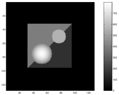
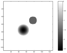
Figure 2: Simulated phantom: magnitude image on the left-hand side (lhs) and phase image on the right-hand side (rhs). We have selected two ROIs: ROI1 is the central square and ROI2 is the blunt flow area (upper right circle).

For the direct problem, i.e simulating the acquired data, the exact model has been used without any approximation, which allows to compute the value of the $k$-space data along any sampling trajectory. A data set of 6 spiral arms of 512 samples each have been simulated, thus the number of samples ($6\times 512$) was 5 folds less than the number of pixels ($128\times 128$). The reduced number of samples and their very irregular density makes the reconstruction problem non invertible and thus allowed to test the quality of the regularized reconstruction in the case of sparse data.

The hyperparameters, chosen empirically to obtain the best possible reconstruction, have been set to following values: $\lambda_{1}=0.1$, $\alpha_{1}=20$, $\lambda_{0}=0.5$ and $\alpha_{0}=10$ and were then also used for the phantom reconstruction. A $7\times 7$ Kaiser-Bessel kernel, as introduced in [6], was used for the gridding reconstruction.

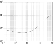
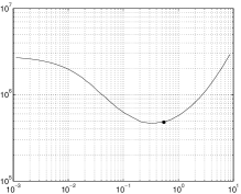
a) $\lambda_{1}$	b) $\lambda_{0}$
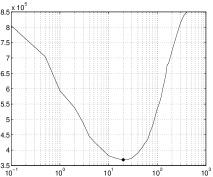
c) $\alpha_{1}$	d) $\alpha_{0}$

Figure 3: Sensitivity to hyperparameters around the chosen values $\lambda_{1}=0.1$, $\alpha_{1}=20$, $\lambda_{0}=0.5$ and $\alpha_{0}=10$: reconstruction errors when one hyperparameter is varied at a time. Case for 6 spirals and 512 samples/spiral (noise free), selected values are indicated (as dots) on each curve.

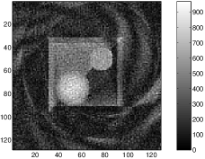
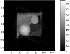
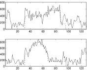
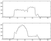
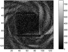
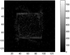
Figure 4: Reconstruction for noisy data (30 dB): 6 spirals and 512 samples/spiral: re-gridding method (lhs) and proposed one (rhs). The top part shows the modulus images, middle part shows rows 50 and 75 and bottom one shows difference images with the reference.

It can be observed that the regularized reconstruction offers a better visual quality than the gridding (Fig. 4) and that it is closer to the reference image. Sharp edges are maintained and enhanced while at the same time the noise level is smoothed throughout the image. This trade-off is achieved by the properties of the selected penalization function. The reconstruction presents less artifacts inside and outside the inner part of the image while the spatial resolution is preserved. These aliasing artifacts due to the undersampling are greatly reduced but their structure is more complex to analyze than for a Cartesian acquisition due to the characteristics of the spiral sampling trajectory [31].

The examination of the $k$-space of the reconstructed images (FFT of the reconstructed images), shown in Fig. 5, allows to compare the frequency content of the two reconstructed images versus the reference one. The proposed method restores a $k$-space very close to the reference one, while the gridding reconstruction still lets appear the underneath sampling trajectory. This shows that the a priori introduced by the regularization is more pertinent and helps to restore an image closer to the original object.

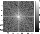
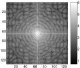
Figure 5: From left to right : reference $k$-space, gridding $k$-space and reconstructed $k$-space (6 spirals and 512 samples/spiral).

Figure 6 presents a quantitative validation of the method, varying the number of spirals, the number of samples per spiral and the SNR, using the following criteria.

• The quadratic reconstruction error in ROI1 (see Fig. 2) which gives a measure of the distance between the reconstruction and the reference.

• The variance for the constant gray level region of ROI2 (see Fig. 2) [13].

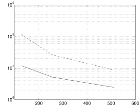
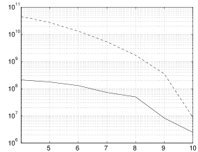
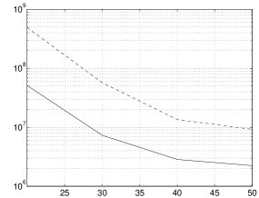
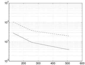
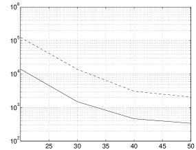
Figure 6: First row: quadratic reconstruction error in ROI1 and second row : variance in ROI2. The gridding method results are plotted with a dotted line and the proposed method results with a solid line. From left to right: 10 spirals, variable number of samples (128, 256 et 512), no noise; variable number of spirals (4 to 10), 512 samples/spiral, no noise; 10 spirals, 512 samples/spiral, variable noise level (20 to 50 dB).

These figures confirm the former qualitative results. The proposed method gives a quadratic error 5 to 300 folds lower than the gridding, while the variance is improved 3 to 10 folds whatever the sampling or noise level.

Figure 3 presents a quantitative evaluation of the hyperparameter sensitivity computed as the variations of the squared reconstruction error in a defined region of interest (ROI1). We note that the selected values are very close to the ones that minimize the errors when only one hyperparameter is varied at a time. The intervals where these parameters can be chosen are relatively large: this ensures that the solution is robust with respect to the hyperparameter values.

This results show that the quality of the image can be maintained while using acquisition sequences that sample a smaller number of data and then reduce the acquisition time, proportionally to the number of acquired spirals.

4.2 Phantom acquisition

The method was then tested on the GEMS test phantom with a 1.5 Tesla Signa system. The sampling trajectory consisted in 24 interleaved spirals each of 2048 samples and a 16 cm FOV.

Figure 7 presents the reconstructed magnitude images (256 $\times$ 256) for the gridding and the regularized methods as well as a zoom in the comb like ROI for the genuine acquisition geometry (24 spirals). Fig. 8 presents the corresponding results when one spiral over two has been discarded, providing a gain of two in the acquisition time.

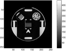
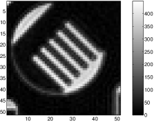
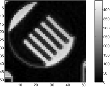
Figure 7: Reconstruction with 24 spirals and 2048 samples/spiral. From top to bottom : modulus image, ROI. On the left the gridding reconstruction and on the right the proposed method.

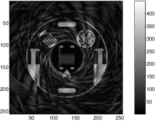
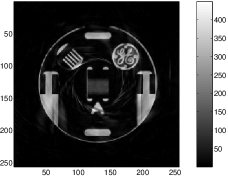
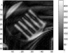
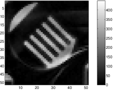
Figure 8: Reconstruction with 12 spirals and 2048 samples/spiral. From top to bottom: modulus image, ROI. On the left the gridding reconstruction and on the right the proposed method.

For the genuine acquisition geometry (Fig. 7) the regularized image is very close to the gridding reconstruction and it even shows a slight reduction of the noise level in the background.

Undersampling strongly degrades the gridding reconstruction (Fig. 8): only a small central region remains free of all artifacts. As has been shown for simulated data, our method applied to actual measurements gives an image where the aliasing artifacts are strongly reduced inside the object and where a very homogeneous background is preserved. The two comb-like ROIs (Fig. 8) show more clearly the improvement provided by the proposed method. The regularization also provides an image with well defined edges, illustrating that the chosen prior is well suited to achieve the compromise between noise smoothing and contour preservation constraints.

Characterization of aliasing artifacts can be approached by studying the structure of the matrix $G$ which can be interpreted as the point spread function of the imaging system: the observed image being the convolution of the true object with $G$. Fig. 9 shows this matrix for the two sampling schemes. The central white spot (resp. peak in the 1D figures) introduces a blurring effect proportional to its diameter (resp. width), while the outer circles (resp. peaks) are responsible for aliasing. The closer these circles to the center the more important the aliasing artifacts. The undersampling that shrinks these circles was partially inverted by the proposed method while it was kept unchanged by the gridding reconstruction.

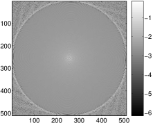
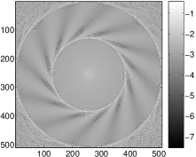
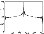
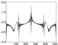
Figure 9: Matrix $G$ for 24 spirals (lhs) and 12 spirals (rhs) (Log scale). Sharp peaks denoted by arrows cause aliasing.

Beforehand computation of matrices $D$ and $G$ considerably speeds up the optimization procedure. However, if $G$ can be computed once for all for a given acquisition sequence, $D$ must be computed for each data set. The computational complexity that arises in computing $D$ is not a drawback for clinical use of the method: it takes 30 sec to compute matrix $D$ (12 spirals, 2048 samples per spiral, image $256\times 256$) using a C-Program on a PC computer with an AMD-Athlon 2.1 GHz processor.

The optimization was performed using the computing environment Matlab in 3 minutes, and 50 iterations were needed to converge to an accurate solution. Each iteration requires one gradient and three criterion calculations. The calculations of the FFTs represent the main computational burden during the minimization: every iteration involves six $512\times 512$ 2D-FFTs for the criterion and two $768\times 768$ 2D-FFTs for the gradient. This time could be considerably reduced by implementing the algorithm on a dedicated processor. Indeed, given the characteristics of the Texas Instruments TMS320C64x series DSP, all of the FFTs could, theoretically, be performed in about 18 sec, leading to an important decrease in the total optimization time.

Moreover the computation of the criterion, the gradient and the matrix $D$ are highly amenable to parallelization, and with a sufficient number of processing elements, the reconstruction could be done even faster, which could allow the use of the method in a wide variety of clinical applications.

5 Discussion / Conclusion

The proposed method differs from more conventional ones insofar as it does not involve any regridding of the acquired data and accounts for edge preserving smoothing penalties. Utilization of only the acquired data and integration of smoothness and edge preservation penalization in the reconstruction opens the way to strong improvement in MRI.

From a computational stand point, the original formulation leads to the awkward situation of an optimization algorithm permanently shifting from Fourier to image domains requiring for numerous heavy non-uniform Fourier transform computations. Rewriting the criterion allowed to perform the whole optimization in the image domain providing the pre-computation of two matrices. The first one characterizes the geometry of acquisitions in $k$-space and gives interpretation of aliasing structures; the second can be seen as a discrete Fourier transform of the acquired data.

Moreover, alternatives exist to still improve the reconstruction efficiency of the method: substituting non-uniform FFT algorithms for the non-uniform Fourier transform in the pre-computations [32]; calculating a solution corresponding to a small ROI only; substituting a Newton like [33] or a dual optimization [34] method to the conjugate gradient could dramatically reduce the computational cost and make the method available for clinical applications.

Finally, the inverted model could be improved by integrating an exponential term that takes into account the relaxation of the magnetic moments. A Laplace inversion framework should then be substituted for the present Fourier framework but the overall inversion procedure will remain valid.

Acknowledgement  — The authors express their gratitude to M.J. Graves, University of Cambridge and Addenbrooke’s Hospital, Cambridge, UK, for providing the acquisitions, fundamental for proposed evaluations.

Appendix

The appendix gives detailed calculi for the new form of the fit to the data term ${\mathcal{J}}_{\mathrm{\scriptscriptstyle LS}}$ and its gradient, required for efficient numerical optimization.

Appendix A Criterion calculus

We have:

$${\mathcal{J}}_{\mathrm{\scriptscriptstyle LS}}({\mathb{f}})=\sum_{l=0}^{L-1}|s_{l}-y_{l}|^{2}=\sum_{l=0}^{L-1}|s_{l}|^{2}+|y_{l}|^{2}-2\Re\{s_{l}\,y_{l}^{*}\}\,.$$ (9)

where $y_{l}={\mathb{h}}_{l}{\mathb{f}}$ is the noise free model output given by Eq (2). It is the sum of quadratic terms over the whole acquired data. The first term is simply the norm of the data, the second one is developed in subsection A.1 and the last one in subsection A.2.

A.1 Term involving model output $y_{l}$

Expansion of $|y_{l}|^{2}$, given model (2) yields:

$$|y_{l}|^{2} = \frac{1}{N^{2}}\left|\,\sum_{p,q=0}^{N-1}f_{p,q}\,{\mathrm{e}}^{i2\pi(k_{x}^{l}p+k_{y}^{l}q)}\right|^{2}$$

$$= \frac{1}{N^{2}}\sum_{q,q,p^{\prime},q^{\prime}=0}^{N-1}f_{p,q}\,f_{p^{\prime},q^{\prime}}^{*}\,{\mathrm{e}}^{i2\pi[k_{x}^{l}(p-p^{\prime})+k_{y}^{l}(q-q^{\prime})]}\,.$$

A change of the summation variable : $u=p-p^{\prime}$ and $v=q-q^{\prime}$ gives:

$$|y_{l}|^{2}=\frac{1}{N^{2}}\sum_{u,v=1-N}^{N-1}\mathop{\sum_{p={\mathrm{m}}(u)}^{p={\mathrm{M}}(u)}}_{q={\mathrm{m}}(v)}^{q={\mathrm{M}}(v)}f_{p,q}\,f_{p-u,q-v}^{*}\,{\mathrm{e}}^{i2\pi(k_{x}^{l}u+k_{y}^{l}v)}$$

where ${\mathrm{m}}(\cdot)$ and ${\mathrm{M}}(\cdot)$ are the index summation bounds:

$${\mathrm{m}}(w)=\begin{cases}|w|&\textrm{if}~{}w\geq 0\cr 0&\textrm{if}~{}w\leq 0\end{cases}$$

and

$${\mathrm{M}}(w)=\begin{cases}N-1&\textrm{if}~{}w\geq 0\cr N-1-|w|&\textrm{if}~{}w\leq 0\end{cases}$$

We then introduce the image correlation matrix :

$$C_{u,v}=\mathop{\sum_{p={\mathrm{m}}(u)}^{p={\mathrm{M}}(u)}}_{q={\mathrm{m}}(v)}^{q={\mathrm{M}}(v)}f_{p,q}\,f_{p-u,q-v}^{*}$$

which can be computed by FFT. So, $|y_{l}|^{2}$ simply writes:

$$|y_{l}|^{2}=\frac{1}{N^{2}}\sum_{v,u=1-N}^{N-1}C_{u,v}\,{\mathrm{e}}^{i2\pi(k_{x}^{l}u+k_{y}^{l}v)}\,.$$

The summation over $l$ yields

$$\sum_{l=0}^{L-1}|y_{l}|^{2} = \frac{1}{N^{2}}\sum_{l=0}^{L-1}\sum_{v,u=1-N}^{N-1}C_{u,v}\,{\mathrm{e}}^{i2\pi(k_{x}^{l}u+k_{y}^{l}v)}$$

$$= \frac{1}{N^{2}}\sum_{v,u=1-N}^{N-1}C_{u,v}\sum_{l=0}^{L-1}{\mathrm{e}}^{i2\pi(k_{x}^{l}u+k_{y}^{l}v)}$$

after rearrangement of the summations. Let us state for $u,v=1-N,\dots,N-1$:

$$G_{u,v}=\frac{1}{N^{2}}\sum_{l=0}^{L-1}{\mathrm{e}}^{i2\pi(k_{x}^{l}u+k_{y}^{l}v)}$$ (10)

which only depends upon the $k$-space trajectory. We finally have:

$$\sum_{l=0}^{L-1}|y_{l}|^{2}=\sum_{v,u=1-N}^{N-1}C_{u,v}\,G_{u,v}\,.$$ (11)

A.2 Term involving model output $y_{l}$ and observed data $s_{l}$

Using (2), the involved term writes:

$$s_{l}\,y_{l}^{*}=s_{l}\frac{1}{N}\sum_{p,q=0}^{N-1}f_{p,q}^{*}\,{\mathrm{e}}^{-i2\pi(k_{x}^{l}p+k_{y}^{l}q)}$$

and summation over $l$ yields:

$$\sum_{l=0}^{L-1}s_{l}\,y_{l}^{*} = \frac{1}{N}\sum_{l=0}^{L-1}s_{l}\sum_{p,q=0}^{N-1}f_{p,q}^{*}\,{\mathrm{e}}^{-i2\pi(k_{x}^{l}p+k_{y}^{l}q)}$$

$$= \frac{1}{N}\sum_{p,q=0}^{N-1}f_{p,q}^{*}\sum_{l=0}^{L-1}s_{l}\,{\mathrm{e}}^{-i2\pi(k_{x}^{l}p+k_{y}^{l}q)}$$

after rearrangement. We then introduce the DFT, for $p,q=0,\dots,N-1$:

$$D_{p,q}=\frac{1}{N}\sum_{l=0}^{L-1}s_{l}\,{\mathrm{e}}^{-i2\pi(k_{x}^{l}p+k_{y}^{l}q)}$$ (12)

which depends upon observed data and $k$-space trajectory. The current term then simply writes:

$$\sum_{l=0}^{L-1}s_{l}\,y_{l}^{*}=\sum_{p,q=0}^{N-1}f_{p,q}^{*}\,D_{p,q}\,.$$ (13)

Substitution of (13) and (11) in (9) yields the announced form of Eq. (6).

Appendix B Gradient of the Criterion

The partial derivative of (13) with respect to $f_{nm}$ clearly writes:

$$\frac{\partial}{\partial f_{nm}}\sum_{l=0}^{L-1}s_{l}\,y_{l}^{*}=\frac{\partial}{\partial f_{nm}}\sum_{p,q=0}^{N-1}f_{p,q}^{*}\,D_{p,q}=D_{n,m}$$

The partial derivative of (11) with respect to $f_{nm}$ is more complicated.

$$\frac{\partial}{\partial f_{nm}}\sum_{v,u=1-N}^{N-1}C_{u,v}\,G_{u,v}$$

$$= \frac{2}{N^{2}}\sum_{l=0}^{L-1}\,{\mathrm{e}}^{-i2\pi(k_{x}^{l}m+k_{y}^{l}n)}\sum_{n^{\prime},m^{\prime}=0}^{N-1}f_{n^{\prime},m^{\prime}}\,{\mathrm{e}}^{i2\pi(k_{x}^{l}m^{\prime}+k_{y}^{l}n^{\prime})}$$

$$= \frac{2}{N^{2}}\sum_{l=0}^{L-1}\sum_{n^{\prime},m^{\prime}=0}^{N-1}f_{n^{\prime},m^{\prime}}\,{\mathrm{e}}^{i2\pi[k_{x}^{l}(m^{\prime}-m)+k_{y}^{l}(n^{\prime}-n)]}$$

Finally, we can write, using the expressions of the matrices $D$ and $G$:

$$\frac{\partial}{\partial f_{nm}}\sum_{v,u=1-N}^{N-1}C_{u,v}\,G_{u,v}$$

$$= \frac{2}{N^{2}}\sum_{l=0}^{L-1}\sum_{u,v=1-N}^{N-1}f_{n-v,m-u}\,{\mathrm{e}}^{-i2\pi(k_{x}^{l}u+k_{y}^{l}v)}$$

$$= 2\sum_{u,v=1-N}^{N-1}f_{n-v,m-u}\,G_{v,u}^{*}.$$

where $G^{*}$ is the conjugate of $G$.

The total gradient using a matrix formulation, is given then as:

$$\frac{\partial{\mathcal{J}}_{\mathrm{\scriptscriptstyle LS}}({\mathb{f}})}{\partial{\mathb{f}}}=2f\star G-2D.$$

where $\star$ is a bidimentional circular-convolution that can be efficiently computed by FFT.

References

- [1] Z. H. Cho, H. S. Kim, H. B. Song, and J. Cumming, “Fourier Transform Nuclear Magnetic Resonance Tomographic Imaging,” Proc. IEEE, vol. 70, no. 10, pp. 1152–1173, 1982.
- [2] H. Meyer, Craig, B. S. Hu, D. G. Nishimura, and A. Macovski, “Fast Spiral Coronary Artery Imaging,” Magn. Reson. Med., vol. 28, pp. 202–213, 1992.
- [3] J. G. Pipe and P. Menon, “Sampling Density Compensation in MRI: Rationale and an Iterative Numerical Solution,” J. Magn. Reson. Imaging, vol. 41, pp. 179–186, 1999.
- [4] G. H. Glover and J. M. Pauly, “Projection reconstruction techniques for reduction of motion effects in MRI,” Magn. Reson. Med., vol. 28, pp. 275–289, 1992.
- [5] H. Azhari, O. E. Denisova, A. Montag, and E. P. Shapiro, “Circular Sampling : Perspective of a Time-Saving Scanning Procedure,” J. Magn. Reson. Imaging, vol. 14, no. 6, pp. 625–631, 1996.
- [6] J. D. O’Sullivan, “A Fast Sinc Function Gridding Algorithm for Fourier Inversion in Computer Tomography,” IEEE Transactions on Medical Imaging, vol. MI-4, no. 4, pp. 200–207, 1985.
- [7] J. I. Jackson, C. H. Meyer, D. G. Nishimura, and A. Macovski, “Selection of a Convolution Function for Fourier Inversion Using Gridding,” IEEE Trans. Medical Imaging, vol. 10, no. 3, pp. 473–478, 1991.
- [8] N. G. Papadakis, C. T. Adrian, and L. D. Hall, “An Algorithm for Numerical Calculation of the -space Data-Weighting for Polarly Sampled Trajectories: Application to Spiral Imaging,” J. Magn. Reson. Imaging, vol. 15, no. 7, pp. 785–794, 1997.
- [9] K. F. King, and L. Angelos, “SENSE Image Quality Improvement Using Matrix Regularization,” Proceedings of the 9th Annual Meeting of ISMRM, pp. 1771, 2001.
- [10] R. Bammer , M. Auer, S. L. Keeling, M. Augustin, L. A. Stables, R. W. Prokesch, R. Stollberger, M. E. Moseley, and F. Fazekas, “ Diffusion Tensor Imaging Using Single-Shot SENSE-EPI,” Magn. Reson. Med., vol. 48, pp. 128–136, 2002.
- [11] F.-H. Lin, K. K Kwong, J. W. Belliveau, and L. L. Wald, “Parallel Imaging Reconstruction Using Automatic Regularization,” Magn. Reson. Med., vol. 51, pp. 559–567, 2004.
- [12] K. P. Pruessmann, M. Weiger, M. B Scheidegger, and P. K. Boesiger, “SENSE: Sensitivity Encoding for Fast MRI,” Magn. Reson. Med., vol. 42, pp. 952–962, 1999.
- [13] R. M. Henkelman, “Measurement of signal intensities in the presence of noise in MR images,” Med. Phys, vol. 12 (2) Mar/Apr, pp. 232–233, 1985.
- [14] G. Demoment, “Image reconstruction and restoration: Overview of common estimation structure and problems,” IEEE Trans. Acoust. Speech, Signal Processing, vol. assp-37, pp. 2024–2036, December 1989.
- [15] C. Oesterle and J. Hennig, “Improvement of Spatial Resolution of Keyhole Effect Images,” Magn. Reson. Med., vol. 39, pp. 244–250, 1998.
- [16] M. Doyle, G. E. Walsh, E. R. Foster, and M. G. Pohost, “Block Regional Interpolation Scheme for k-Space ( BRISK ): A Rapid Cardiac Imaging Technique,” Magn. Reson. Med., vol. 33, pp. 163–170, 1995.
- [17] M. Doyle, G. E. Walsh, E. R. Foster, and M. G. Pohost, “Rapid Cardiac Imaging with Turbo BRISK,” Magn. Reson. Med., vol. 37, pp. 410–417, 1997.
- [18] F. R. Korosec, R. Frayne, T. M. Grist, and C. A. Mistretta, “Time-resolved contrast-enhanced 3D MR angiography.,” Magn. Reson. Med., vol. 36(3), pp. 345–351, 1996.
- [19] Y. Cao and D. N. Levin, “Using Prior Knowledge of Human Anatomy to Constrain MR Image Acquisition and Reconstruction: Half -space and Full -space Techniques,” J. Magn. Reson. Imaging, vol. 15, No. 6, pp. 669–676, 1997.
- [20] I. Dologlou, D. van Ormondt, and G. Carayannis, “MRI scan time reduction through non-uniform sampling and SVD-based estimation,” Signal Processing, vol. 55, pp. 207–219, 1996.
- [21] G. McGibney, M. R. Smith, S. T. Nichols, and A. Crawley, “Quantitative Evaluation of Several Partiel Fourier Reconstruction Algorithms Used in MRI,” Magn. Reson. Med., vol. 30, pp. 51–59, 1993.
- [22] R. Van de Walle, H. H. Barrett, K. J. Myers, M. I. Altbach, B. Desplanques, A. F. Gmito, J. Cornelis, and I. Lemahieu, “Reconstruction of MR images from data acquired on a general nonregular grid by pseudoinverse calculation,” IEEE Trans. Medical Imaging, vol. 19, no. 12, pp. 1160–1167, 2000.
- [23] Y. Gao and S. J. Reeves, “Optimal -space sampling in MRSI for images with a limited region of support,” IEEE Trans. Medical Imaging, vol. 19, no. 12, pp. 1168–1178, 2000.
- [24] A. Tikhonov and V. Arsenin, Solutions of Ill-Posed Problems. Washington, dc: Winston, 1977.
- [25] B. R. Hunt, “Bayesian methods in nonlinear digital image restoration,” IEEE Trans. Communications, vol. C-26, pp. 219–229, March 1977.
- [26] S. Geman and D. Geman, “Stochastic relaxation, Gibbs distributions, and the Bayesian restoration of images,” IEEE Trans. Pattern Anal. Mach. Intell., vol. PAMI-6, pp. 721–741, November 1984.
- [27] A. Blake and A. Zisserman, Visual reconstruction. Cambridge, ma: The mit Press, 1987.
- [28] S. Geman and D. McClure, “Statistical methods for tomographic image reconstruction,” in Proceedings of the 46th Session of the ici, Bulletin of the ici, vol. 52, pp. 5–21, 1987.
- [29] H. R. Künsch, “Robust priors for smoothing and image restoration,” Ann. Inst. Stat. Math., vol. 46, no. 1, pp. 1–19, 1994.
- [30] W. H. Press, S. A. Teukolsky, W. T. Vetterling, and B. P. Flannery, Numerical recipes in C, the art of scientific computing. New York: Cambridge Univ. Press, 2nd ed., 1992.
- [31] H. Sedarat, A. B. Kerr, J. M. Pauly, and D. Nishimura, “Partial-FOV Reconstruction in Dynamic Spiral Imaging,” Magn. Reson. Med., vol. 43, pp. 439–439, 2000.
- [32] B. Dale, M. Wendt, and J. L. Duerk, “A rapid look-up table method for reconstructing MR images from arbitrary -space trajectories,” IEEE Trans. Medical Imaging, vol. 20, no. 3, pp. 207–217, 2001.
- [33] D. P. Bertsekas, Nonlinear programming. Belmont, ma: Athena Scientific, 2nd ed., 1999.
- [34] J. Idier, “Convex half-quadratic criteria and interacting auxiliary variables for image restoration,” IEEE Trans. Image Processing, vol. 10, pp. 1001–1009, July 2001.