Dirac operators on cobordisms: degenerations and surgery

Abstract.

We investigate the Dolbeault operator on a pair of pants, i.e., an elementary cobordism between a circle and the disjoint union of two circles. This operator induces a canonical selfadjoint Dirac operator $D_{t}$ on each regular level set $C_{t}$ of a fixed Morse function defining this cobordism. We show that as we approach the critical level set $C_{0}$ from above and from below these operators converge in the gap topology to (different) selfadjoint operators $D_{\pm}$ that we describe explicitly. We also relate the Atiyah-Patodi-Singer index of the Dolbeault operator on the cobordism to the spectral flows of the operators $D_{t}$ on the complement of $C_{0}$ and the Kashiwara-Wall index of a triplet of finite dimensional lagrangian spaces canonically determined by $C_{0}$.

Introduction

Suppose $(M,g)$ is compact oriented odd dimensional Riemann manifold. We let $\widehat{M}$denote the cylinder $[0,1]\times M$ and $\hat{g}$ denote the cylindrical metric $dt^{2}+g$.

Let $\hat{D}$ be a first order elliptic operator operator on $\widehat{M}$ that has the form

$$\widehat{D}={\sigma}(dt)\bigl{(}\,\nabla_{t}-D(t)\,\bigr{)}, {\dagger}$$ ()

where ${\sigma}$ denotes the principal symbol of $\widehat{D}$, and for every $t\in[0,1]$ the operator $D(t)$ on $\{t\}\times M$ is elliptic and symmetric. For simplicity we assume that both $A(0)$ and $A(1)$ are invertible.

A classical result of Atiyah, Patodi and Singer [2, §7] (see also [12, §17.1]) relates the index $i_{APS}(\widehat{A})$ of the Atiyah-Patodi-Singer problem associated to $\widehat{D}$ to the spectral flow $SF(\,D(t)\,)$ of the family of Fredholm selfadjoint operators $D(t)$. More precisely, they show that

$$i_{APS}(\widehat{D})+SF\bigl{(}\,D(t),\;0\leq t\leq 1\,\bigr{)}=0.$$ (A)

We can regard the cylinder $\widehat{M}$ as a trivial cobordism between $\{0\}\times M$ and $\{1\}\times M$, and the coordinate $t$ as a Morse function on $\widehat{M}$ with no critical points.

In this paper we initiate an investigation of the case when $\widehat{M}$ is no longer a trivial cobordism. We outline below the main themes of this investigation.

First, we will concentrate only on elementary cobordisms, the ones that trace a single surgery. We regard such a cobordism as a pair $(\widehat{M},f)$, where $\widehat{M}$ is an even dimensional, compact oriented manifold with boundary, and $f$ is a Morse function on $\widehat{M}$ with a single critical point $p_{0}$ such that

$$f(\widehat{M})=[-1,1],\;\;f(\partial M)=\{-1,1\},\;\;f(p_{0})=0.$$

We set $M_{\pm}:=f^{-1}(\pm 1)$ so that we have a diffeomorphism of oriented manifolds $\partial M=M_{+}\cup-M_{-}$. By removing the critical level set $M_{0}=f^{-1}(0)$ we obtain two cylinders

$$\widehat{M}_{-}=\{f<0\}\cong[-1,0)\times M_{-},\;\;\widehat{M}_{+}=\{f>0\}\cong(0,1]\times M_{+}.$$

Suppose $\hat{g}$ is a Riemann metric on $\widehat{M}$ and $\widehat{D}:C^{\infty}(E_{+})\rightarrow C^{\infty}(E_{-})$ is a Dirac type operator on $\widehat{M}$, where $E_{+}\oplus E_{-}$ is a ${\mathbb{Z}}/2$-graded bundle of Clifford modules.

Using the bundle isomorphism ${\sigma}(dt)$ we can regard $\widehat{D}$ as an operator $C^{\infty}(E_{+})\rightarrow C^{\infty}(E_{+})$. As explained in [8] (see also Section 2 of this paper), for every $t\neq 0$, there is a canonically induced symmetric Dirac operator $D(t)$ on the slice $M_{t}=f^{-1}(t)$. We regard $D(t)$ as a linear operator $D(t):C^{\infty}(E_{+}|_{M_{t}})\rightarrow C^{\infty}(E_{+}|_{M_{t}})$, so that if $\hat{g}$ were a cylindrical metric then formula (${\dagger}$ ‣ Introduction) would hold.

The Riemann metric $\hat{g}$ defines finite measures $dV_{t}$ on all the slices $M_{t}$, including the singular slice $M_{0}$. In particular we obtain a one parameter family of Hilbert spaces

$$\boldsymbol{H}_{t}:=L^{2}(M_{t},dV_{t};E_{+}).$$

We can now regard $D(t)$ as a closed, densely defined linear operator on $\boldsymbol{H}_{t}$.

Problem 1. Organize the family $(\boldsymbol{H}_{t})_{t\in[-1,1]}$ as a trivial Hilbert bundle over the interval $[-1,1]$

$$\mathcal{H}=\boldsymbol{H}\times[-1,1]\rightarrow[-1,1].$$

Under reasonable assumptions on $f$ and $\hat{g}$ we can use the gradient flow of $f$ to address this issue. Once this problem is solved we can regard the operators $D(t)$, $t\neq 0$ as closed densely defined operators on the same Hilbert space $\boldsymbol{H}$. We can then formulate our next problem.

Problem 2. Investigate whether the limits

$$SF_{-}:=\lim_{{\varepsilon}\searrow 0}SF(\,D(t),-1\leq t\leq-{\varepsilon}),\;\;SF_{+}:=\lim_{{\varepsilon}\searrow 0}SF(\,D(t),\;{\varepsilon}\leq t\leq 1\,).$$

exist and are finite.

If Problem 2 has a positive answer we are interested in a version of (A) relating these limits to the Atiyah-Patodi-Singer index of $\widehat{D}$ in the noncylindrical formulation of [8, 9].

Problem 3. Express the quantity

$$\delta:=i_{APS}(\widehat{D})+SF_{-}+SF_{+}$$ (B)

in terms of invariants of the singular level set $M_{0}$.

The existence of the limits in Problem 2 is a consequence of a much more refined analytic behavior of the family of operators $D(t)$ that we now proceed to explain. We set

$$\widehat{\boldsymbol{H}}:=\boldsymbol{H}\oplus\boldsymbol{H},\;\;{\boldsymbol{H}}_{+}=\boldsymbol{H}\oplus 0,\;\;{\boldsymbol{H}}_{-}=0\oplus\boldsymbol{H},$$

and denote by $\mathrm{Lag}$ the Grassmannian of hermitian lagrangian subspaces $\widehat{\boldsymbol{H}}$. These are complex subspaces $L\subset\widehat{\boldsymbol{H}}$ satisfying $L^{\perp}=JL$, where $J:\boldsymbol{H}\oplus\boldsymbol{H}\rightarrow\boldsymbol{H}\oplus\boldsymbol{H}$ is the operator with block decomposition

$$J=\left[\begin{array}[]{cc}0&-1\\ 1&0\end{array}\right].$$

Following [5] we denote by $\mathrm{Lag}^{-}$ the open subset of $\mathrm{Lag}$ consisting of lagrangians $L$ such that the pair of subspaces $(L,\widehat{\boldsymbol{H}}_{-})$ is a Fredholm pair, i.e.,

$$L+{\boldsymbol{H}}_{-}\;\;\mbox{is closed and}\;\;\dim L\cap{\boldsymbol{H}}_{-}<\infty$$

As explained in [5], the space $\mathrm{Lag}^{-}$ equipped with the gap topology of [10, §IV.2] is a classifying spaces for the complex $K$-theoretic functor $K^{1}$.

To a closed densely defined operator $T:\operatorname{Dom}(T)\subset\boldsymbol{H}\rightarrow\boldsymbol{H}$ we associate its switched graph

$$\widetilde{\Gamma}_{T}:=\Bigl{\{}(Th,h)\in\widehat{\boldsymbol{H}};\;\;h\in\operatorname{Dom}(T)\,\Bigr{\}}.$$

Then $T$ is selfadjoint if and only if $\widetilde{\Gamma}_{T}\in\mathrm{Lag}$. It is also Fredholm if and only if $\widetilde{\Gamma}_{T}\in\mathrm{Lag}^{-}$. We can now formulate a refinement of Problem 2.

Problem $\mathbf{2^{*}}$. Investigate whether the limits $\widetilde{\Gamma}_{\pm}=\lim_{t\searrow 0}\widetilde{\Gamma}_{D(\pm t)}$ exist in the gap topology and, if so, do they belong to $\mathrm{Lag}^{-}$.

The gap convergence of the switched graphs of operators is equivalent to the convergence in norm as $t\rightarrow 0^{\pm}$ of the resolvents $R_{t}=(\boldsymbol{i}+D(t)\,)^{-1}$. To show that $\widetilde{\Gamma}_{\pm}\in\mathrm{Lag}^{-}$ it suffices to show that the limits $R_{\pm}=\lim_{t\rightarrow 0^{\pm}}R_{t}$ are compact operators. If in addition $\widetilde{\Gamma}_{\pm}\cap\widehat{\boldsymbol{H}}_{-}=0$ then the limits in Problem 2 exist and are finite.

An even analog of Problem $2^{*}$ was investigated in [16]. The role of the smooth slices $M_{t}$ was played there by a $1$-parameter family of Riemann surfaces degenerating to a Riemann surface with single singularity of the simplest type, a node. The authors show that the gap limit of the graphs of Dolbeault operators on $M_{t}$ exists and then described it explicitly.

In this paper we solve Problems 1, $2^{*}$ and 3 in the symplest possible case, when $\widehat{M}$ is an elementary $2$-dimensional cobordism, i.e., a pair of pants (see Figure 1) and $\widehat{D}$ is the Dolbeault operator on the Riemann surface $\widehat{M}$.

We solved Problem 1 by an ad-hoc intuitive method. The limits $\widetilde{\Gamma}_{\pm}$ in Problem $2^{*}$ turned out to be switched graphs of certain Fredholm-selfadjoint operators $D_{\pm}$, $\widetilde{\Gamma}_{\pm}=\widetilde{\Gamma}_{D_{\pm}}$.

We describe these operators as realizations of two different boundary value problems associated to the same symmetric Dirac operator $D_{0}$ defined on the disjoint union of four intervals. These intervals are obtained by removing the singular point of the critical level set $M_{0}$ and then cutting in two each of the resulting two components. The boundary conditions defining $D_{\pm}$ are described by some ($4$-dimensional) lagrangians $\Lambda_{\pm}$ determined by the geometry of the singular slice $M_{0}$. The operators $D_{\pm}$ have well defined eta invariants $\eta_{\pm}$. If $\ker D_{\pm}=0$ then we can express the defect $\delta$ in (B) as

$$\delta=\frac{1}{2}\bigl{(}\,\eta_{-}-\eta_{+}\,\bigr{)}.$$ (C)

The above difference of eta invariants admits a purely symplectic interpretation very similar to the signature additivity defect of Wall [19]. More precisely, we show that

$$\delta=-\omega(\,\Lambda_{0}^{\perp},\Lambda_{+},\Lambda_{-}\,\bigr{)},$$ (D)

where $\Lambda_{0}$ is the Cauchy data space of the operator $D_{0}$ and $\omega(L_{0},L_{1},L_{2})$ denotes the Kashiwara-Wall index of a triplet of lagrangians canonically determined by $M_{0}$; see [4, 11, 19] or Section 4.

Here is briefly how we structured the paper. In Section 1 we investigate in great detail the type of degenerations that occur in the family $D(t)$ as $t\rightarrow 0^{\pm}$. It boils down to understanding the behavior of families of operators of the unit circle $S^{1}$ of the type

$$L_{\varepsilon}=-\boldsymbol{i}\frac{d}{d\theta}+a_{\varepsilon}(\theta),$$

where $\{a_{\varepsilon}\}_{{\varepsilon}>0}$ is a family of smooth functions on the unit circle that converges in a rather weak sense way as ${\varepsilon}\rightarrow 0$ to a Dirac measure supported at a point $\theta_{0}$. For example if we think of $a_{\varepsilon}$ as densities defining measures converging weakly to the Dirac measure, then the corresponding family of operators has a well defined gap limit; see Corollary 1.5.

In Theorem 1.8 we give an explicit description of this limiting operator as an operator realizing a natural boundary value problem on the disjoint union of the two intervals, $[0,\theta_{0}]$ and $[\theta_{0},2\pi]$. This section also contains a detailed discussion of the eta invariants of operators of the type $-\boldsymbol{i}\frac{d}{d\theta}+a(\theta)$, where $a$ is a allowed to be the “density” of any finite Radon measure.

In Section 2 we survey mostly known facts concerning the Atiyah-Patodi-Singer problem when the metric near the boundary is not cylindrical. Because the various orientation conventions vary wildly in the existing literature, we decided to go careful through the computational details. We discuss two topics. First, we explain what is the restriction of a Dirac operator to a cooriented hypersurface and relate this construction to another conceivable notion of restriction. In the second part of this section we discuss the noncylindrical version of the Atiyah-Patodi-Singer index theorem. Here we follow closely the presentation in [8, 9].

In Section 3 we formulate and prove the main result of this paper, Theorem 3.5. The solution to Problem $2^{*}$ is obtained by reducing the study of the degenerations to the model degenerations investigated in Section 1 The equality (C) follows immediately from the noncyclindrical version of the Atiyah-Patodi-Singer index theorem discussed in Section 2 and the eta invariant computations in Section 1. In the last section we present a few facts about the Kashiwara-Wall triple index and then use them to prove (D). Our definition of triple index is the one used by Kirk and Lesch [11] that generalizes to infinite dimensions.

Finally a few words about conventions and notation. We consistently orient the boundaries using the outer-normal-first convention. We let $\boldsymbol{i}$ stand for $\sqrt{-1}$ and we let $L^{k,p}$ denote Sobolev spaces of functions that have weak derivatives up to order $k$ that belong to $L^{p}$.

1. A model degeneration

Let $L>0$ be a positive number. Denote by $\boldsymbol{H}$ the Hilbert space $L^{2}([0,L],{\mathbb{C}})$. To any smooth function $a:{\mathbb{R}}\rightarrow{\mathbb{R}}$ which is $L$-periodic we associate the selfadjoint operator

$$D_{a}:\operatorname{Dom}(D_{a})\subset\boldsymbol{H}\rightarrow\boldsymbol{H},$$

where

$$\operatorname{Dom}(D_{a})=\bigl{\{}\,u\in L^{1,2}([0,L],{\mathbb{C}});\;\;u(0)=u(L)\,\bigr{\}},\;\;D_{a}u=-\boldsymbol{i}\frac{du}{dt}+au.$$ (1.1)

In this section we would like to understand the dependence of $D_{a}$ on the potential $a$, and in particular, we would like to allow for more singular potentials such as a Dirac distribution concentrated at an interior point of the interval. We will reach this goal via a limiting procedure that we implement in several steps.

We observe first that $D_{a}$ can be expressed in terms of the resolvent $R_{a}:=(\boldsymbol{i}+D_{a})^{-1}$ as $D_{a}=R_{a}^{-1}-\boldsymbol{i}$. The advantage of this point of view is that we can express $R_{a}$ in terms of the more regular function

$$A(t):=\int_{0}^{t}a(s)ds. \ast$$ ()

which continues to make sense even when there is no integrable function $a$ such that ($\ast$ ‣ 1) holds. For example, we can allow $A(t)$ to be any function with bounded variation so that, formally, $a$ ought to be the density of any Radon measure on $[0,L]$.

This will allow us to conclude that when we have a family of smooth potentials $a_{n}$ that converge in a suitable sense to something singular such as a Dirac function, then the operators $D_{a_{n}}$ have a limit in the gap topology to a Fredholm selfadjoint operator with compact rezolvent. We show that in many cases this limit operator can be expressed as the Fredholm operator defined by a boundary value problem.

We begin by expressing $R_{a}$ as an integral operator. We set

$$A(t):=\int_{0}^{t}a(s)ds,\;\;\Phi_{A}(t):=\boldsymbol{i}A(t)-t.$$

For $f\in H$ the function $u=R_{a}f$ is the solution of the boundary value problem

$$\Bigl{(}\,\boldsymbol{i}-\boldsymbol{i}\frac{d}{dt}\,\Bigr{)}u+au=f,\;\;u(0)=u(L).$$

We rewrite the above equation as

$$\frac{du}{dt}+(\boldsymbol{i}a-1)u=\boldsymbol{i}f$$

from which we deduce

$$\frac{d}{dt}\Bigl{(}\,e^{\Phi_{A}(t)}u(t)\,\Bigr{)}=\boldsymbol{i}e^{\Phi_{A}(t)}f(t).$$

This implies that

$$e^{\Phi_{A}(t)}u(t)-u(0)=\boldsymbol{i}\int_{0}^{t}e^{\Phi_{A}(s)}f(s)ds,\;\;\forall t\in[0,L].$$

If in the above equality we let $t=L$ and use condition $u(0)=u(L)$ we deduce

$$u(0)=\frac{\boldsymbol{i}}{e^{\Phi_{A}(L)}-1}\int_{0}^{L}e^{\Phi_{A}(s)}f(s)ds.$$

Finally we deduce

$$u(t)=R_{a}f=\frac{\boldsymbol{i}e^{-\Phi_{A}(t)}}{e^{\Phi_{A}(L)}-1}\int_{0}^{L}e^{\Phi_{A}(s)}f(s)ds+\boldsymbol{i}\int_{0}^{t}e^{-(\Phi_{A}(t)-\Phi_{A}(s)}f(s)ds.$$ (1.2)

The key point of the above formula is that $R_{a}$ can be expressed in terms of the antiderivative $A(t)$ which typically has milder singularities than $a$. To analyze the dependence of $R_{a}$ on $A$ we introduce a class of admissible functions.

Definition 1.1.

(a) We say that $A:[0,L]\rightarrow{\mathbb{R}}$ is admissible if $A$ has bounded variation, it is right continuous, and $A(0)=0$. We denote by $\mathcal{A}$ or $\mathcal{A}_{L}$ the class of admissible functions.

(b) We say that a sequence $\{A_{n}\}_{n\geq 0}\subset\mathcal{A}$ converges very weakly to $A\in\mathcal{A}$ if there exists a negligible subset $\Delta\subset(0,L)$ such that

$$\lim_{n\rightarrow\infty}A_{n}(t)=A(t),\;\;\forall t\in[0,L]\setminus\Delta. \hbox to0.0pt{$\sqcap$\hss}\sqcup$$

Remark 1.2.

(a) Note that if $A_{n}$ converges very weakly to $A$ then $A_{n}(L)$ converges to $A(L)$.

(b) Let us explain the motivation behind the “very weak” terminology. An admissible function $A$ defines a finite Lebesgue-Stieltjes measure $\mu_{A}$ on $[0,L]$, and the resulting map $A\mapsto\mu_{A}$ is a linear isomorphism between $\mathcal{A}$ and the space of finite Borel measures on $[0,L]$, [7, Thm. 3.29]. Thus, we can identify $\mathcal{A}$ with the space of finite Borel measures on $[0,L]$. As such it is equipped with a weak topology.

According to [6, §4.22], a sequence of Borel measures $\mu_{A_{n}}$ is weakly convergent to $\mu_{A}$ if and only if $\mu_{A_{n}}(\mathcal{O})\rightarrow\mu_{A}(\mathcal{O})$, for any (relatively) open subset $\mathcal{O}$ of $[0,L]$. This clearly implies the very weak convergence introduced in Definition $\hbox to0.0pt{$\sqcap$\hss}\sqcup$ ‣ 1.1. $\hbox to0.0pt{$\sqcap$\hss}\sqcup$

Inspired by (1.2) we define for every $A\in\mathcal{A}$ the function $\Phi_{A}(t)=\boldsymbol{i}A(t)-t$ and the integral kernels

$$\mathcal{S}_{A}:[0,L]\times[0,L]\rightarrow{\mathbb{C}},\;\;\mathcal{S}_{A}(t,s)=\frac{\boldsymbol{i}}{e^{\Phi_{A}(L)}-1}e^{-\bigl{(}\,\Phi_{A}(t)-\Phi_{A}(s)\,\bigr{)}},\;\;\forall t,s\in[0,L],$$

$$\mathcal{K}_{A}:[0,L]\times[0,L]\rightarrow{\mathbb{C}},\;\;\mathcal{K}_{A}(t,s)=\begin{cases}0&t<s\\ \boldsymbol{i}e^{-\bigl{(}\,\Phi_{A}(t)-\Phi_{A}(s)\,\bigr{)}}&t\geq s.\end{cases}$$

Observe that there exists a constant $C>0$ such that

$$\|\mathcal{S}_{A}\|_{L^{\infty}([0,L]\times[0,L])}+\|\mathcal{K}_{A}\|_{L^{\infty}([0,L]\times[0,L])}\leq C,\;\;\forall A\in\mathcal{A}.$$ (1.3)

Thus, these kernels define bounded compact operators $S_{A},K_{A}:\boldsymbol{H}\rightarrow\boldsymbol{H}$; see [18, §X.2]. Moreover, if we denote by $\|\bullet\|_{\rm op}$ the operator norm on the space $\mathcal{B}(\boldsymbol{H})$ of bounded linear operators $\boldsymbol{H}\rightarrow\boldsymbol{H}$ then we have the estimates that

$$\|S_{A}\|_{\rm op}\leq\|\mathcal{S}_{A}\|_{L^{2}([0,L]\times[0,L])},\;\;\|K_{A}\|_{\rm op}\leq\|\mathcal{K}_{A}\|_{L^{2}([0,L]\times[0,L])}.$$ (1.4)

We can now rewrite (1.2) as

$$R_{a}=R_{A}:=S_{A}+K_{A}.$$ (1.5)

Proposition 1.3.

If $A_{n}$ converges very weakly to $A$ then $S_{A_{n}}$ and $K_{A_{n}}$ converge in the operator norm topology to $S_{A}$ and respectively $K_{A}$.

Proof.

The very weak convergence implies that

$$\mathcal{S}_{A_{n}}(t,s)\stackrel{{\scriptstyle k\rightarrow\infty}}{{{\longrightarrow}}}\mathcal{S}_{A}(t,s),\;\;\mathcal{K}_{A_{n}}(t,s)\stackrel{{\scriptstyle k\rightarrow\infty}}{{{\longrightarrow}}}\mathcal{K}_{A}(t,s)\;\;\mbox{a.e. on $[0,L]\times[0,L]$}.$$

Using (1.3), the above pointwise convergence and the dominated convergence theorem we deduce

$$\lim_{n\rightarrow\infty}\Bigl{(}\,\|\mathcal{S}_{A_{n}}-\mathcal{S}_{A}\|_{L^{2}([0,L]\times[0,L])}+\|\mathcal{K}_{A_{n}}-\mathcal{K}_{A}\|_{L^{2}([0,L]\times[0,L])}\,\Bigr{)}=0.$$

Using (1.4) we deduce that

$$\lim_{n\rightarrow\infty}\Bigl{(}\,\|S_{A_{n}}-S_{A}\|_{\rm op}+\|S_{A_{n}}-S_{A}\|_{\rm op}\,\Bigr{)}=0.$$

$\hbox to0.0pt{$\sqcap$\hss}\sqcup$

We want to describe the spectral decompositions of the operators $R_{A}$, $A\in\mathcal{A}$. To do this we rely on the fact that for certain $A$’s the operator $R_{A}$ is the resolvent of an elliptic selfadjoint operator on $S^{1}$. We use this to produce an intelligent guess for the spectrum of $R_{A}$ in general.

Let $a$ be a smooth, real valued, $L$-period function on ${\mathbb{R}}$ and form again the operator $D_{a}$ defined in (1.1). We set as usual

$$A(t)=\int_{0}^{t}a(s)ds.$$

The operator $D_{a}$ has discrete real spectrum. If $u(t)$ is an eigenfunction corresponding to an eigenvalue $\lambda$ then

$$-\boldsymbol{i}\frac{du}{dt}+au=\lambda u\Rightarrow\frac{du}{dt}+i(a-\lambda)u=0$$

so that $u(t)=u(0)e^{-\boldsymbol{i}A(t)+\boldsymbol{i}\lambda t}$. The periodicity assumption implies $\lambda L-A(L)\in 2\pi{\mathbb{Z}}$ so the spectrum of $D_{a}$ is

$$\operatorname{spec}(D_{a})=\left\{\,\lambda_{A,n}:=\frac{2\pi}{L}\bigl{(}\,\omega_{A}+n\,\bigr{)};\;\;n\in{\mathbb{Z}}\,\right\},\;\;\mbox{where}\;\;\omega_{A}:=\frac{A(L)}{2\pi}.$$ (1.6)

The eigenvalue $\lambda_{A,n}$ is simple and the eigenspace corresponding to $\lambda_{A,n}$ is spanned by

$$\psi_{A,n}(t):=e^{\frac{2\pi n\boldsymbol{i}t}{L}}e^{-\boldsymbol{i}(A(t)-\frac{A(L)t}{L})}.$$

The numbers $\lambda_{A,n}$ and the functions $\psi_{A,n}$ are well defined for any $A\in\mathcal{A}$.

Lemma 1.4.

Let $A\in\mathcal{A}$. Then the collection $\{\psi_{A,n}(t);\;\;n\in{\mathbb{Z}}\}$ defines a Hilbert basis of $\boldsymbol{H}$.

Proof.

Observe first that the collection

$$e_{n}(t)=\psi_{A=0,n}(t)=e^{\frac{2\pi n\boldsymbol{i}t}{L}},\;\;n\in{\mathbb{Z}}$$

is the canonical Hilbert basis of $\boldsymbol{H}$ that leads to the classical Fourier decomposition. The map

$$U_{A}:\boldsymbol{H}\rightarrow\boldsymbol{H},\;\;\boldsymbol{H}\ni f(t)\mapsto e^{-\boldsymbol{i}(A(t)-\frac{A(L)t}{L})}f(t)$$

is unitary. It maps $e_{n}$ to $\psi_{A,n}$ which proves our claim. $\hbox to0.0pt{$\sqcap$\hss}\sqcup$

A direct computation shows that

$$R_{A}\psi_{A,n}=\frac{1}{\boldsymbol{i}+\lambda_{A,n}}\psi_{A,n},\;\;\forall A\in\mathcal{A},\;\;A\in\mathcal{A}.$$

This proves that for any $A\in\mathcal{A}$ the collection $\{\psi_{A,n}\}_{n\in{\mathbb{Z}}}$ is a Hilbert basis that diagonalizes the operator $R_{A}$. Observe that $R_{A}$ is injective and compact. We define

$$T_{A}:=R_{A}^{-1}-\boldsymbol{i}.$$

The operator $T_{A}$, is unbounded, closed and densely defined with domain $\operatorname{Dom}(T_{A})={\rm Range}\,(R_{A})$. We will present later a more explicit description of $\operatorname{Dom}(T_{A})$ for a large class of $A$’s.

Note that when

$$A=\int_{0}^{t}a(s)ds,\;\;\mbox{$a$ smooth and $L$-periodic},$$

the operator $T_{A}$ coincides with the operator $D_{a}$ defined in (1.1). Proposition 1.3 can be rephrased as follows.

Corollary 1.5.

If the sequence $(A_{n})_{n\geq 1}\subset\mathcal{A}$ converges very weakly to $A\in\mathcal{A}$ then the sequence of unbounded operators $(T_{A_{n}})_{n\geq 1}$ converges in the gap topology to the unbounded operator $T_{A}$. $\hbox to0.0pt{$\sqcap$\hss}\sqcup$

The spectrum of $T_{A}$ consists only of the simple eigenvalues $\lambda_{A,n}$, ${n\in{\mathbb{Z}}}$. The function $\psi_{A_{n}}$ is an eigenfunction of $T_{A}$ corresponding to the eigenvalue $\lambda_{A,n}$. The eta invariant of $T_{A}$ is now easy to compute. For $s\in{\mathbb{C}}$ we have

$$\eta_{A}(s):=\sum_{\lambda>0}\frac{1}{\lambda^{s}}\Bigl{(}\dim\ker(\lambda-T_{A})-\dim\ker(\lambda+T_{A})\,\Bigr{)}$$

$$=\sum_{n\in{\mathbb{Z}}\setminus\{-\omega_{A}\}}\frac{\operatorname{sign}\lambda_{A,n}}{|\lambda_{A,n}|^{s}}=\frac{L^{s}}{2\pi^{s}}\sum_{n\in{\mathbb{Z}}\setminus\{-\omega_{A}\}}\frac{\operatorname{sign}\bigl{(}\,n+\omega_{A}\bigr{)}}{|n+\omega_{A}|^{s}}.$$

Let

$$\rho_{A}:=\omega_{A}-\lfloor\omega_{A}\rfloor=\frac{A(L)}{2\pi}-\left\lfloor\frac{A(L)}{2\pi}\,\right\rfloor\in[0,1).$$ (1.7)

If $\rho_{A}=0$ then $\eta_{A}(s)=0$ because in this case the spectrum of $T_{A}$ is symmetric about the origin. If $\rho_{A}\neq 0$ then we have

$$\eta_{A}(s)=\frac{L^{s}}{2\pi^{s}}\Biggl{(}\,\sum_{n\geq 0}\frac{1}{(n+\rho_{A})^{s}}-\sum_{n\geq 0}\frac{1}{(n+1-\rho_{A})^{s}}\,\Biggr{)}=\frac{L^{s}}{2\pi^{s}}\Bigl{(}\,\zeta(s,\rho_{A})-\zeta(s,1-\rho_{A})\,\Bigr{)},$$

where for every $a\in(0,1]$ we denoted by $\zeta(s,a)$ the Riemann-Hurwitz zeta function

$$\zeta(s,a)=\sum_{n\geq 0}\frac{1}{(n+a)^{s}}.$$

The above series is convergent for any $s\in{\mathbb{C}}$, $\operatorname{{\bf Res}}>1$ and admits an analytic continuation to the puctured plane ${\mathbb{C}}\setminus\{s=1\}$. Its value at the origin $s=0$ is given by Hermite’s formula [17, 13.21]

$$\zeta(0,a)=\frac{1}{2}-a.$$ (1.8)

We deduce that $\eta_{A}(s)$ has an analytic continuation at $s=0$ and we have

$$\eta_{A}(0)=\left\{\begin{array}[]{ccl}0&{\rm if}&\rho_{A}=0,\\ 1-2\rho_{A}&{\rm if}&\rho_{A}\in(0,1).\end{array}\right.$$ (1.9)

If we introduce the function

$$\xi_{A}=\frac{1}{2}\bigl{(}\,\dim\ker T_{A}+\eta_{A}(0)\,\bigr{)},$$

then we can rewrite the above equality in a more compact way

$$\xi_{A}=\frac{1}{2}(1-2\rho_{A})=\frac{1}{2}-\rho_{A}.$$ (1.10)

Suppose we have $A_{0},A_{1}\in\mathcal{A}$. We set $A_{s}=A_{0}+s(A_{1}-A_{0})\in\mathcal{A}$. The map $[0,1]\ni s\mapsto A_{s}\in\mathcal{A}$ is continuous in the weak tooplogy on $\mathcal{A}$ and thus the family of operators $T_{A_{s}}$ is continuous with respect to the gap topology. The eigenvalues of the family $T_{A_{s}}$ can be organized in smooth families

$$\lambda_{s,n}=\frac{2\pi}{L}(\omega_{s}+n)=\frac{2\pi}{L}\Bigl{(}\omega_{A_{0}}+s\bigl{(}\,\omega_{1}-\omega_{0}\,\bigr{)}+n\,\Bigr{)},\;\;\omega_{s}:=\omega_{A_{s}},;\;\forall s\in[0,1].$$

Assume for simplicity that $\omega_{0},\omega_{1}\not\in{\mathbb{Z}}$, i.e., the operators $T_{A_{0}}$ and $T_{A_{1}}$ are invertible. Denote by $SF(A_{1},A_{0})$ the spectral flow of the affine family $T_{A_{s}}$. Then

$$SF(A_{1},A_{0})=\#\{n\in{\mathbb{Z}};\;\;\omega_{0}+n<0,\;\;\omega_{1}+n>0\}-\#\{n\in{\mathbb{Z}};\;\;\omega_{0}+n>0,\;\;\omega_{1}+n<0\}$$

$$=\#\Bigl{(}{\mathbb{Z}}\cap(\omega_{0},\omega_{1})\,\Bigr{)}-\#\Bigl{(}{\mathbb{Z}}\cap(\omega_{1},\omega_{0})\,\Bigr{)}.$$

We conclude

$$SF(A_{1},A_{0})=\bigl{(}\,\lfloor\omega_{1}\rfloor-\lfloor\omega_{0}\rfloor\,\bigr{)},\;\;\omega_{i}=\frac{A_{i}(L)}{2\pi}.$$ (1.11)

Using (1.10) we deduce

$$SF(A_{1},A_{0})=\lfloor\omega_{A_{1}}\rfloor-\lfloor\omega_{A_{0}}\rfloor=\omega_{A_{1}}-\omega_{A_{0}}+\bigl{(}\,\xi_{A_{1}}-\xi_{A_{0}}\,\bigr{)}.$$ (1.12)

Remark 1.6 (Rescaling trick).

Note that the rescaling

$$[0,L_{1}]\ni\tau\mapsto t=\frac{\tau}{c}\in[0,L_{0}],\;\;c=\frac{L_{1}}{L_{0}}.$$

induces an isometry $\mathcal{I}_{L_{1},\mathcal{L}_{0}}:\boldsymbol{H}_{L_{0}}=L^{2}(0,L_{0};{\mathbb{C}})\rightarrow\boldsymbol{H}_{L_{1}}=L^{2}(0,L_{1};{\mathbb{C}})$,

$$\boldsymbol{H}_{L_{0}}\ni f(t)\mapsto\mathcal{I}_{L_{1},L_{0}}f(\tau):=c^{1/2}f\left(\frac{\tau}{c}\,\right)\in\boldsymbol{H}_{L_{1}}.$$

The unbounded operator $\frac{d}{dt}$ on $\boldsymbol{H}_{L_{0}}$ is the conjugate to the operator $c\frac{d}{d\tau}$ on $\boldsymbol{H}_{L_{1}}$.

If $\alpha(t)$ is a real bounded measurable function on $[0,L_{0}]$, then the bounded operator on $\boldsymbol{H}_{L_{0}}$ defined by pointwise multiplication by $\alpha(t)$ is conjugate to the bounded operator on $\boldsymbol{H}_{L_{1}}$ defined by the multiplication by $a(\tau)=\alpha(\tau/c)$. Hence the unbounded operator $D_{b}$ on $\boldsymbol{H}_{L_{0}}$ is conjugate to the unbounded operator $cD_{c^{-1}a}$ on $\boldsymbol{H}_{L_{1}}$,

$$cD_{c^{-1}a}=\mathcal{I}_{L_{1},L_{0}}D_{\alpha}\mathcal{I}_{L_{1},L_{0}}^{-1}.$$ (1.13)

Its resolvent is obtained by solving the periodic boundary value problem

$$\boldsymbol{i}u+c\left(-\boldsymbol{i}\frac{d}{d\tau}+c^{-1}a(\tau)\right)u(\tau)=f(\tau),\;\;u(0)=u(L_{1}),$$

or equivalently

$$\frac{d}{d\tau}u+c^{-1}\bigl{(}\,a(\tau)-\boldsymbol{i}\,\bigr{)}u=c^{-1}\boldsymbol{i}f,\;\;u(0)=u(L_{1}).$$

If we set

$$A(\tau)=\int_{0}^{\tau}a({\sigma})d{\sigma}\;\;\mbox{and}\;\;\Phi_{A,c}(t)=c^{-1}\Phi_{A}(\tau)=c^{-1}(\boldsymbol{i}A(\tau)-\tau),$$

then we see that $R_{\alpha}$ is conjugate to the integral operator $R_{A,c}$

$$R_{A,c}f(\tau)=\frac{c^{-1}\boldsymbol{i}e^{-\Phi_{A,c}(\tau)}}{e^{\Phi_{A,c}(L_{1})}-1}\int_{0}^{L_{1}}e^{\Phi_{A,c}({\sigma})}f(s)ds+c^{-1}\boldsymbol{i}\int_{0}^{t}e^{-(\Phi_{A,c}(\tau)-\Phi_{A}({\sigma})}f({\sigma})d{\sigma}.$$

Arguing exactly as in the proof of Proposition 1.3 we deduce that if $A_{n}$ coverges very weakly to $A\in\mathcal{A}_{L_{1}}$ and the sequence of positive numbers $c_{n}$ converges to the positive number $c$ then $R_{A_{n},c_{n}}$ converges in the operator norm to $R_{A,c}$.

For any $c>0$ and $A\in\mathcal{A}$ we define the operator

$$T_{A,c}=R_{A,c}^{-1}-\boldsymbol{i},\;\;c>0.$$

Note that $T_{A,c}=cT_{c^{-1}A}$. Then for every $c>0$ the spectrum of $T_{A,c}$ is

$$\operatorname{spec}\bigl{(}\,T_{A,c}\,\bigr{)}=c\operatorname{spec}\bigl{(}\,T_{c^{-1}A}\,\bigr{)}. \hbox to0.0pt{$\sqcap$\hss}\sqcup$$

We want to give a more intuitive description of the operators $R_{A}$, and $T_{A}$ for a large class of $A$’s. We begin by introducing a nice subclass $\mathcal{A}_{*}$ of $\mathcal{A}$. Let $H(t)$ denote the Heaviside function

$$H(t)=\begin{cases}1,&t\geq 0\\ 0,&t<0.\end{cases}$$

Definition 1.7.

We say that $A\in\mathcal{A}$ is nice if there exists $a\in L^{\infty}(0,L)$, a finite subset ${\mathcal{P}}\subset(0,L)$, and a function $c:{\mathcal{P}}\rightarrow{\mathbb{R}}$ such that if we define

$$A_{*}(t):=\int_{0}^{t}a(s)ds$$

then

$$A(t)=A_{*}(t)+\sum_{p\in\Delta}c(p)H(t-p),\;\;\forall t\in[0,L].$$

We denote by $\mathcal{A}_{*}$ the subcollection of nice functions. $\hbox to0.0pt{$\sqcap$\hss}\sqcup$

Let us first point out that $\mathcal{A}_{*}$ is a vector subspace of $\mathcal{A}$. Next, observe that $A\in\mathcal{A}^{*}$ if and only if there exists a finite subset ${\mathcal{P}}_{A}\subset(0,L)$ such that the restriction of $A$ to $[0,L]\setminus{\mathcal{P}}$ is Lipschitz continuous. In this case $A$ admits left and right limits at any point $t\in[0,L]$ and we define

$$c:{\mathcal{P}}_{A}\rightarrow{\mathbb{R}},\;\;c(p)=\lim_{t\searrow p}A(t)-\lim_{t\nearrow p}A(t).$$

Then

$$A_{*}(t)=A(t)-\sum_{p\in{\mathcal{P}}}c(p)H(t-p)$$

is Lipschitz continuous, it is differentiable a.e. on $[0,L]$ and we define $a$ to be the derivative of $A_{*}$.

Let us next observe that if $A\in\mathcal{A}_{*}$ then the operator $T_{A}$ can be informally described as

$$T_{A}=-\boldsymbol{i}\frac{d}{dt}+a(t)+\sum_{p\in{\mathcal{P}}_{A}}c(p)\delta_{p}.$$

In other words, $T_{A}$ would like to be a Dirac type operator whose coefficients are measures. In the above informal discussion we left out a description of the domain of $T_{A}$. Below we would like to give a precise description of $T_{A}$ as a closed unbounded selfadjoint operator defined by an elliptic boundary value problem.

For any partition of $[0,L]$, ${\mathcal{P}}=\{0<t_{1}<\cdots<t_{n-1}<L\}$, we set

$$t_{0}:=0,\;\;t_{n}:=L,\;\;I_{k}:=[t_{k-1},t_{k}],\;\;k=1,\dotsc,n.$$

We define the Hilbert space

$$\boldsymbol{H}_{\mathcal{P}}=\bigoplus_{k=1}^{n}L^{2}(I_{k},{\mathbb{C}}),$$

and the Hilbert space isomorphism

$$\mathcal{I}_{\mathcal{P}}:\boldsymbol{H}\rightarrow\boldsymbol{H}_{\mathcal{P}},\;\;\boldsymbol{H}\ni f\mapsto\bigl{(}\,f|_{I_{1}},\dotsc,f|_{I_{n}}\,\bigr{)}\in\boldsymbol{H}_{\mathcal{P}}.$$

Let $A\in\mathcal{A}_{*}$ and ${\mathcal{P}}$ be a partition

$${\mathcal{P}}=\{0<t_{1}<\cdots<t_{n-1}<L\}$$

that contains the set of discontinuities of $\mathcal{A}$, ${\mathcal{P}}\supset{\mathcal{P}}_{A}$. We set

$$a=\frac{dA_{*}}{dt},\;\;;a_{k}=a|_{I_{k}},\;k=1,\dotsc,n.$$

For $j=1,\dotsc,n-1$ we denote by $c_{j}=c_{j}(A)$ the jump of $A$ at $t_{j}$,

$$c_{j}=A(t_{j}^{+})-A(t_{j}^{-}).$$

Finally we define the closed unbounded linear operator

$$L_{\mathcal{A},{\mathcal{P}}}:\operatorname{Dom}(L_{A,{\mathcal{P}}})\subset\boldsymbol{H}_{\mathcal{P}}\rightarrow\boldsymbol{H}_{\mathcal{P}},$$

where $\operatorname{Dom}(L_{A,{\mathcal{P}}})$ consists of $n$-uples $(u_{k})_{1\leq k\leq n}\in\boldsymbol{H}_{\mathcal{P}}$ such that

$$u_{k}\in L^{1,2}(I_{k}),\;\;k=1,\dotsc,n,$$ (1.14a)

$$u_{j+1}(t_{j})=e^{-\boldsymbol{i}c_{j}}u_{j}(t_{j}),\;\;j=1,\dotsc,n-1,$$ (1.14b)

$$u_{n}(L)=u_{1}(0).$$ (1.14c)

and

$$L_{A,{\mathcal{P}}}(u_{1},\dotsc,u_{n})=\Bigl{(}\,-\boldsymbol{i}\frac{du_{1}}{dt}+a_{1}u_{1},\dotsc,-\boldsymbol{i}\frac{du_{n}}{dt}+a_{n}u_{n}\,\Bigr{)}.$$ (1.15)

A standard argument shows that $L_{A,{\mathcal{P}}}$ is closed, densely defined and selfadjoint. In particular, the operator $(L_{A,{\mathcal{P}}}+\boldsymbol{i})$ is invertible, with bounded inverse.

Theorem 1.8.

For any $A\in\mathcal{A}_{*}$ and any partition

$${\mathcal{P}}=\{0<t_{1}<\cdots<t_{n-1}<L\}$$

that contains the set of discontinuities of $\mathcal{A}$ we have the equality

$$L_{A,{\mathcal{P}}}=\mathcal{I}_{\mathcal{P}}T_{A}\mathcal{I}_{\mathcal{P}}^{-1}.$$

Proof.

For simplicity we write $L_{A}$ instead of $L_{A,{\mathcal{P}}}$. We will prove the equivalent statement

$$(\boldsymbol{i}+L_{A})^{-1}=\mathcal{I}_{\mathcal{P}}(T_{A}+\boldsymbol{i})^{-1}\mathcal{I}_{\mathcal{P}}^{-1}=\mathcal{I}_{\mathcal{P}}R_{A}\mathcal{I}_{{\mathcal{P}}}^{-1}.$$

In other words we have to prove that for any $u,f\in\boldsymbol{H}$ if $u=R_{A}f$, then $u\in\operatorname{Dom}(L_{A})$ and $(L_{A}+\boldsymbol{i})\mathcal{I}_{\mathcal{P}}u=\mathcal{I}_{\mathcal{P}}f$. More precisely, we have to show that the collection $\mathcal{I}_{A}u=(u_{k})_{1\leq k\leq n}$ satisfies (1.14a–1.14c) and (1.15). Using (1.2) we deduce

$$u(t)=\frac{\boldsymbol{i}e^{-\Phi_{A}(t)}}{e^{\Phi_{A}(L)}-1}\int_{0}^{L}e^{\Phi_{A}(s)}f(s)ds+\boldsymbol{i}e^{-\Phi_{A}(t)}\int_{0}^{t}e^{\Phi_{A}(s)}f(s)ds.$$ (1.16)

This implies the condition (1.14a). The condition (1.15) follows by direct computation using (1.16).

Next, we observe that

$$u(t_{j}^{+})=\frac{\boldsymbol{i}e^{-\Phi_{A}(t_{j}^{+})}}{e^{\Phi_{A}(L)}-1}\int_{0}^{L}e^{\Phi_{A}(s)}f(s)ds+\boldsymbol{i}e^{-\Phi_{A}(t_{j}^{+})}\int_{0}^{t_{j}}e^{\Phi_{A}(s)}f(s)ds,$$

$$u(t_{j}^{-})=\frac{\boldsymbol{i}e^{-\Phi_{A}(t_{j}^{-})}}{e^{\Phi_{A}(L)}-1}\int_{0}^{L}e^{\Phi_{A}(s)}f(s)ds+\boldsymbol{i}e^{-\Phi_{A}(t_{j}^{-})}\int_{0}^{t_{j}}e^{\Phi_{A}(s)}f(s)ds,$$

from which we conclude that

$$u(t_{j}^{+})=e^{-\boldsymbol{i}\bigl{(}\,\Phi_{A}(t_{j}^{+})-\Phi_{A}(t_{j}^{-})\,\bigr{)}}u(t_{j}^{-}),\;\;\forall j=1,\dotsc n-1.$$

This proves (1.14b). The equality (1.14c) follows directly from (1.5). $\hbox to0.0pt{$\sqcap$\hss}\sqcup$

Remark 1.9.

We would like to place the above operator $L_{A}$ in a broader perspective that we will use extensively in Section 4. Consider a compact, oriented $1$-dimensional manifold with boundary $I$. In other words $I$ is a disjoint union of finitely many compact intervals

$$\boldsymbol{I}=\sqcup_{k=1}^{n}I_{k}.$$

If $I_{k}:=[a_{k},b_{k}]$, $a_{k}<b_{k}$, then we set

$$\partial_{+}I_{k}:=\{b_{k}\},\;\;\partial_{-}I_{k}:=\{a_{k}\},\;\;\partial_{+}\boldsymbol{I}:=\{b_{1},\dotsc,b_{n}\},\;\;\partial_{-}\boldsymbol{I}:=\{a_{1},\dotsc,a_{n}\}.$$

In particular, we have a direct sum decomposition of (finite dimensional) Hilbert spaces

$$\boldsymbol{E}:=L^{2}(\partial I,{\mathbb{C}})=L^{2}(\partial_{+}\boldsymbol{I})\oplus L^{2}(\partial_{-}\boldsymbol{I})=:\boldsymbol{E}_{+}\oplus\boldsymbol{E}_{-}.$$

On the space $C^{\infty}(\boldsymbol{I},{\mathbb{C}})$ of smooth complex valued functions on $\boldsymbol{I}$ we have a canonical, symmetric Dirac $\mathcal{D}$ operator described on each $I_{k}$ by $-\boldsymbol{i}\frac{d}{dt}$. Let $\sigma$ denote the principal symbol of this operator. If $\boldsymbol{\nu}_{*}$ denotes the outer conormal to the boundary. We then get an operator

$$J={\sigma}(\boldsymbol{\nu}_{*}):L^{2}(\partial\boldsymbol{I},{\mathbb{C}})\rightarrow L^{2}(\partial\boldsymbol{I},{\mathbb{C}}).$$

It is a unitary operator satisfying $J^{2}=-1$, $\ker(\boldsymbol{i}+J)=\boldsymbol{E}_{+}$, and $\ker(\boldsymbol{i}-J)=\boldsymbol{E}_{-}$. It thus defines a Hermitian symplectic structure in the sense of [1, 5, 14]. A (hermitian) lagrangian subspace of $\boldsymbol{E}$ is then a complex subspace $L$ such that $L^{\perp}=JL$. We denote by $\mathrm{Lag}(\boldsymbol{E},J)$ the Grassmannin of hermitian lagrangian spaces. We denote by $\operatorname{Iso}(\boldsymbol{E}_{+},\boldsymbol{E}_{-})$ the space of linear isometries $\boldsymbol{E}_{+}\rightarrow\boldsymbol{E}_{-}$. As explained in [1] there exists a natural bijection

$$\operatorname{Iso}(\boldsymbol{E}_{+},\boldsymbol{E}_{-})\rightarrow\mathrm{Lag}(\boldsymbol{E}),\;\;\operatorname{Iso}(\boldsymbol{E}_{+},\boldsymbol{E}_{-})\ni T\longmapsto\Gamma_{T}$$

where $\Gamma_{T}$ is the graph of $T$ viewed as a subspace of $\boldsymbol{E}$. Our spaces $\boldsymbol{E}_{\pm}$ are equipped with natural bases and through these bases we can identify $\operatorname{Iso}(\boldsymbol{E}_{+},\boldsymbol{E}_{-})$ with the unitary group $U(n)$. We denote by $\Delta$ the Lagrangian subspace corresponding to the identity operator.

Any subspace $V\subset\boldsymbol{E}$ defines a Fredholm operator

$$\mathcal{D}_{V}:\operatorname{Dom}(\mathcal{D}_{V})\subset L^{2}(\boldsymbol{I},{\mathbb{C}})\rightarrow L^{2}(\boldsymbol{I},{\mathbb{C}}),$$

where

$$\operatorname{Dom}(\mathcal{D}_{V})=\bigl{\{}\,u\in L^{1,2}(\boldsymbol{I},{\mathbb{C}});\;\;u|_{\partial I}\in V\,\bigr{\}},\;\;\mathcal{D}_{V}u=\mathcal{D}u.$$

The index of this operator is

$$i_{V}=\dim(V\cap\Delta)-\dim(\Delta\cap JV^{\perp})=\dim(V\cap\Delta)-\dim(J\Delta\cap V^{\perp})$$

$$=\dim(V\cap\Delta)-\dim(\Delta^{\perp}\cap V^{\perp})=\dim V-\operatorname{codim}\Delta=\dim V-n.$$

A simple argument shows that $\mathcal{D}_{V}$ is selfadjoint if and only if $V\in\mathrm{Lag}(\boldsymbol{E})$. As we explained above, in this case $V$ can be identified with the graph of an isometry $T:\boldsymbol{E}_{+}\rightarrow\boldsymbol{E}_{-}$. We say that $T$ is the transmission operator associated to the selfadjoint boundary value problem.

For example, if in Theorem 1.8 we let $A(t)=\sum_{j=1}^{n-1}c_{j}H(t-t_{j})$, then we see that the operator $L_{A}$ can be identified with the operator $\mathcal{D}_{\Gamma_{T}}$, where the transmission operator $T\in\operatorname{Iso}(\boldsymbol{E}_{+},\boldsymbol{E}_{-})$ is given by the unitary $n\times n$ matrix

$$T=\left[\begin{array}[]{llrccc}0&0&0&\cdots&0&1\\ e^{-\boldsymbol{i}c_{1}}&0&0&\cdots&0&0\\ 0&e^{-\boldsymbol{i}c_{2}}&0&\cdots&0&0\\ \vdots&\vdots&\vdots&\vdots&\vdots&\vdots\\ \cdot&\cdot&\cdot&\cdot&\cdot&\cdot\\ 0&0&0&\cdots&e^{-\boldsymbol{i}c_{n-1}}&0\end{array}\right].$$

$\hbox to0.0pt{$\sqcap$\hss}\sqcup$

2. The Atiyah-Patodi-Singer theorem

We review here the Atiyah-Patodi-Singer index theorem for Dirac operators on manifold with boundary, when the metric is not assumed to be cylindrical near the boundary. Our presentation follows closely, [8, 9], but we present a few more details since the various orientation conventions and the terminology in [8, 9] are different from those in [3, 13] that we use throughout this paper.

Suppose $(\widehat{M},\hat{g})$ is a compact, oriented Riemann, and $M\subset\widehat{M}$ be a hypersurface in $\widehat{M}$ co-oriented by a unit normal vector field $\boldsymbol{\nu}$ along $M$. Let $n:=\dim M$ so that $\dim\widehat{M}=n+1$. We denote by $g$ the induced metric on $M$. We first want to define a canonical restriction to $M$ of a Dirac operator on $\hat{M}$.

Let $\exp^{\hat{g}}:T\widehat{M}\rightarrow\widehat{M}$ denote the exponential map determined by the metric $\hat{H}$. For sufficiently small ${\varepsilon}>0$ the map

$$(-{\varepsilon},{\varepsilon})\times M\ni(t,p)\mapsto\exp^{\hat{g}}_{p}\bigl{(}\,t\boldsymbol{\nu}(p)\,\bigr{)}\in\widehat{M}$$

is a diffeomorphism onto a small open tubular neighborhood $\mathcal{O}_{\varepsilon}$ of $M$. The metric $g$ determines a cylindrical metric $dt^{2}+g$ on $(-{\varepsilon},{\varepsilon})\times M$. Via the above diffeomorphism we get a metric $\hat{g}_{0}$ on $\mathcal{O}_{\varepsilon}$. We say that $\hat{g}_{0}$ is the cylindrical approximation of $\hat{g}$ near $M$.

We denote by $\widehat{\nabla}$ the Levi-Civita connection of the metric $\hat{g}$ and by $\widehat{\nabla}^{0}$ the Levi-Civita connection of the metric $\hat{g}_{0}$. We set

$$\boldsymbol{\Xi}:=\widehat{\nabla}-\widehat{\nabla}^{0}\in\Omega^{1}\bigl{(}\,\mathcal{O}_{\varepsilon},\,\operatorname{End}(\,T\widehat{M}\,)\,\bigr{)}.$$

To get a more explicit description of $\boldsymbol{\Xi}$ we fix a local oriented, $g$-orthonormal frame $(\boldsymbol{e}_{1},\dotsc,\boldsymbol{e}_{n})$ on $M$. Together with the unit normal vector field $\boldsymbol{\nu}$ we obtain a local oriented orthonormal frame $(\boldsymbol{\nu},\boldsymbol{e}_{1},\dotsc,\boldsymbol{e}_{n})$ of $T\widehat{M}|_{M}$. We extend it by parallel transport along the geodesics orthogonal to $M$ to a local, oriented orthonormal frame $(\hat{\boldsymbol{\nu}},\hat{\boldsymbol{e}}_{1},\dotsc,\hat{\boldsymbol{e}}_{n})$ of $T\widehat{M}$.

Denote by $\widehat{\boldsymbol{\omega}}$ the connection form associated to $\widehat{\nabla}$ by this frame, and by $\widehat{\boldsymbol{\theta}}$ the connection form associated to $\widehat{\nabla}^{0}$ by this frame. We can represent both $\widehat{\boldsymbol{\omega}}$ and $\widehat{\boldsymbol{\theta}}$ as skew-symmetric $(n+1)\times(n+1)$ matrices

$$\widehat{\boldsymbol{\omega}}=\bigl{(}\,\widehat{\boldsymbol{\omega}}^{i}_{j}\,\bigr{)}_{0\leq i,j\leq n},\;\;\widehat{\boldsymbol{\theta}}=\bigl{(}\,\widehat{\boldsymbol{\theta}}^{i}_{j}\,\bigr{)}_{0\leq i,j\leq n},$$

where the entries are $1$-forms. Then $\boldsymbol{\Xi}=\widehat{\boldsymbol{\omega}}-\widehat{\boldsymbol{\theta}}$.

We set $\hat{\boldsymbol{e}}_{0}:=\hat{\boldsymbol{\nu}}$, and we denote by $(\hat{\boldsymbol{e}}^{k})_{0\leq k\leq n}$ the dual orthonormal frame of $T^{*}\widehat{M}$.Then we have

$$\hat{\boldsymbol{\omega}}^{i}_{j}=\hat{\boldsymbol{\omega}}^{i}_{kj}\hat{\boldsymbol{e}}^{k},\;\;\hat{\boldsymbol{\theta}}^{i}_{j}=\hat{\boldsymbol{\theta}}^{i}_{kj}\hat{\boldsymbol{e}}^{k},\;\;\widehat{\nabla}_{k}\hat{\boldsymbol{e}}_{j}=\hat{\boldsymbol{\omega}}^{i}_{kj}\hat{\boldsymbol{e}}_{i},\;\;\widehat{\nabla}_{k}^{0}\hat{\boldsymbol{e}}_{j}=\hat{\boldsymbol{\theta}}^{i}_{kj}\hat{\boldsymbol{e}}_{i},\;\;\forall 0\leq j,k\leq n,$$

where we have used Einstein’s summation convention.

Observe that $\widehat{\nabla}^{0}\hat{\boldsymbol{e}}_{0}=0$ so that $\hat{\boldsymbol{\theta}}_{0}^{i}=\hat{\boldsymbol{\theta}}^{0}_{i}=0$. Also,

$$\hat{\boldsymbol{\omega}}^{i}_{jk}=\hat{\boldsymbol{\theta}}^{i}_{jk},\;\;\forall 1\leq i,j,k\leq n.$$

If we write

$$\boldsymbol{\Xi}=\bigl{(}\boldsymbol{\Xi}^{i}_{j}\,\bigr{)}_{0\leq i,j\leq n},\;\;\boldsymbol{\Xi}^{i}_{j}=\boldsymbol{\Xi}^{i}_{jk}\hat{\boldsymbol{e}}^{k},$$

and we let $o(1)$ denote any quantity that vanishes along $M$. then we have

$$\boldsymbol{\Xi}^{i}_{j}=-\boldsymbol{\Xi}^{j}_{i},\;\;\forall 0\leq i,j\leq n,$$ (2.1)

$$\boldsymbol{\Xi}^{i}_{kj}=o(1),\;\;\forall 1\leq i,j\leq n,\;\;0\leq k\leq n.$$ (2.2)

We set

$$\boldsymbol{\Xi}_{kij}:=\boldsymbol{\Xi}^{i}_{kj}=\hat{g}\bigl{(}\widehat{\nabla}_{k}\hat{\boldsymbol{e}}_{j},\hat{\boldsymbol{e}}_{i}\,\bigr{)},\;\;\hat{\boldsymbol{\omega}}_{ij}=\hat{\boldsymbol{\omega}}^{i}_{j},\;\;\hat{\boldsymbol{\theta}}_{ij}=\hat{\boldsymbol{\theta}}^{i}_{j},\;\;\boldsymbol{\omega}_{kij}=\boldsymbol{\omega}^{i}_{kj},\;\;\boldsymbol{\theta}_{kij}=\boldsymbol{\omega}^{i}_{kj}.$$

We denote by $Q$ the second fundamental form of the embedding $M\hookrightarrow\widehat{M}$,

$$Q(e_{i},e_{j})=g(\widehat{\nabla}_{\boldsymbol{e}_{i}}\boldsymbol{\nu},\boldsymbol{e}_{j}).$$

Along the boundary we have the equalities

$$\Xi_{kj0}=\boldsymbol{\Xi}_{jk0}=-\boldsymbol{\Xi}_{k0j}=Q(\boldsymbol{e}_{j},\boldsymbol{e}_{k})\;\;\forall 1\leq i,j\leq n,$$ (2.3a)

$$\Xi_{ij0}=0,\;\;\forall 0\leq i,j\leq n.$$ (2.3b)

To understand the nature of the restriction to a hypersurface of a Dirac operator we begin with a special case. Namely, we assume that $\widehat{M}$ is equipped with a $spin$ structure. We denote by $\hat{{\mathbb{S}}}$ the associated complex spinor bundle so that $\widehat{{\mathbb{S}}}$ is ${\mathbb{Z}}/2$-graded is $\dim\widehat{M}$ is even, and ungraded otherwise. We have a Clifford multiplication

$$\hat{\boldsymbol{c}}:T^{*}M\rightarrow\operatorname{End}(\hat{{\mathbb{S}}}).$$

The metrics $\hat{g}$ and $\hat{g}_{0}$ define connections $\widehat{\nabla}^{spin}$ and $\widehat{\nabla}^{spin,0}$ on $\hat{{\mathbb{S}}}|_{\mathcal{O}_{\varepsilon}}$. Using the local frame $(\hat{\boldsymbol{e}}_{i})_{0\leq i,j\leq n}$ we can write

$$\widehat{\nabla}^{spin}_{k}=\partial_{k}-\frac{1}{4}\hat{\boldsymbol{\omega}}_{kij}\hat{\boldsymbol{c}}(\hat{\boldsymbol{e}}^{i})\hat{\boldsymbol{c}}(\hat{\boldsymbol{e}}^{j}),\;\;\widehat{\nabla}_{k}^{spin,0}=\partial_{k}-\frac{1}{4}\hat{\boldsymbol{\theta}}_{kij}\hat{\boldsymbol{c}}(\hat{\boldsymbol{e}}^{i})\hat{\boldsymbol{c}}(\hat{\boldsymbol{e}}^{j}),$$

where we again use Einstein’s summation convention.

Using the connections $\widehat{\nabla}^{spin}$ and $\widehat{\nabla}^{spin,0}$ we obtain two Dirac operators $\hat{D}$ and respectively $\hat{D}_{0}$ on $\widehat{{\mathbb{S}}}|_{\mathcal{O}_{\varepsilon}}$

$$\hat{D}=\sum_{i=0}^{n}\hat{\boldsymbol{c}}(\hat{e}^{i})\widehat{\nabla}^{spin}_{i},\;\;\hat{D}_{0}=\sum_{i=0}^{n}\hat{\boldsymbol{c}}(\hat{e}^{i})\widehat{\nabla}^{spin,0}_{i}.$$

Identifying $\mathcal{O}_{\varepsilon}$ with $(-{\varepsilon},{\varepsilon})\times M$ we obtain a projection

$$\pi:\mathcal{O}_{\varepsilon}\rightarrow M.$$

We set ${\mathbb{S}}:=\hat{{\mathbb{S}}}|_{M}$. The parallel transport given by $\widehat{\nabla}^{spin}$ yields a bundle isomorphism $\hat{{\mathbb{S}}}|_{\mathcal{O}_{\varepsilon}}\cong\pi^{*}{\mathbb{S}}$. Using these identifications we can rewrite the operators $\hat{D}$ and $\hat{D}_{0}$ as

$$\hat{D}=\hat{\boldsymbol{c}}(\hat{\boldsymbol{e}}_{0})\bigl{(}\,\widehat{\nabla}^{spin}_{0}-D(t)\,\bigr{)}:C^{\infty}(\pi^{*}{\mathbb{S}})\rightarrow C^{\infty}(\pi^{*}{\mathbb{S}}),$$

$$\hat{D}_{0}=\hat{\boldsymbol{c}}(\hat{\boldsymbol{e}}^{0})\bigl{(}\,\partial_{0}-D_{0}(t)):C^{\infty}(\pi^{*}{\mathbb{S}})\rightarrow C^{\infty}(\pi^{*}{\mathbb{S}}).$$

The operators $D(t)$ and $D_{0}(t)$ are first order differential operators $C^{\infty}(\widehat{{\mathbb{S}}}|_{\{t\}\times M})\rightarrow C^{\infty}(\widehat{{\mathbb{S}}}|_{\{t\}\times M})$ and thus can be viewed as $t$-dependent operators on ${\mathbb{S}}$.

The operator $D_{0}(t)$ is in fact independent of $t$ and thus we can identify it with a Dirac operator on $C^{\infty}({\mathbb{S}})\rightarrow C^{\infty}(M)$. It is called the canonical restriction of $\hat{D}$ to $M$, and we will denote it by $\mathcal{R}_{M}(\hat{D})$.This operator is intrinsic to $M$. More precisely when $\dim\widehat{M}$ is even then ${\mathbb{S}}$ is the direct sum of two copies of the spinor bundle on $M$ and the operator $D_{0}$ is the direct sum of two copies of the $spin$-Dirac operator determined by the Riemann metric on $M$.

When $\dim\widehat{M}$ is odd then ${\mathbb{S}}$ is the spinor bundle on $M$ and $D_{0}$ is the $spin$-Dirac operator determined by the metric on the boundary and the induced $spin$ structure. We would like to express $\mathcal{R}_{M}(\hat{D})$ in terms of $D(t)|_{t=0}$.

Let $\boldsymbol{\nu}_{*}:=\hat{\boldsymbol{e}}^{0}\in C^{\infty}\bigl{(}\,T^{*}\widehat{M}|_{\partial\widehat{M}}\,\bigr{)}$, set $J:=\hat{\boldsymbol{c}}(\boldsymbol{\nu}_{*})$ and define $\boldsymbol{c}:T^{*}M\rightarrow\operatorname{End}({\mathbb{S}})$ by setting

$$\boldsymbol{c}(\alpha)=\hat{\boldsymbol{c}}(\,\boldsymbol{\nu}_{*}(p)\,)\hat{\boldsymbol{c}}(\alpha)=J\hat{\boldsymbol{c}}(\alpha),\;\;\forall p\in M,\;\;\alpha\in T^{*}M\subset(T^{*}\widehat{M})|_{M}.$$

Observe first that

$$\mathcal{R}_{M}(\hat{D})=D_{0}(t)=\partial_{0}+J\hat{D}_{0}.$$

Next we observe that

$$\widehat{\nabla}^{spin}-\widehat{\nabla}^{spin,0}=-\frac{1}{4}\sum_{i,j}\boldsymbol{\Xi}_{ij}\hat{\boldsymbol{c}}(\hat{\boldsymbol{e}}^{i})\hat{\boldsymbol{c}}(\hat{\boldsymbol{e}}^{j}).$$

so that

$$\widehat{\nabla}^{spin}_{0}-\widehat{\nabla}^{spin,0}_{0}=\widehat{\nabla}^{spin}_{0}-\partial_{0}=-\frac{1}{4}\Xi_{0ij}J\hat{\boldsymbol{c}}(\hat{\boldsymbol{e}}^{i})\hat{\boldsymbol{c}}(\hat{\boldsymbol{e}}^{j})=o(1),$$

$$\hat{D}-\hat{D}_{0}=-\frac{1}{4}\sum_{i,j,k}\boldsymbol{\Xi}_{kij}\hat{\boldsymbol{c}}(\hat{\boldsymbol{e}}^{k})\hat{\boldsymbol{c}}(\hat{\boldsymbol{e}}^{i})\hat{\boldsymbol{c}}(\hat{\boldsymbol{e}}^{j})=:\mathcal{L}.$$

We denote by $\mathcal{L}(t)$ the restriction of $\mathcal{L}$ to the slice $\{t\}\times M$ so that $\mathcal{L}(t)$ is an endomorphism of $\widehat{{\mathbb{S}}}|_{\{t\}\times M}$.

Hence

$$\hat{D}=J\partial_{0}-JD(t),\;\;D(t)=J\hat{D}+\partial_{0}=J\hat{D}_{0}+\partial_{0}+J\mathcal{L}=D_{0}(t)+J\mathcal{L},$$

so that

$$D(0)=\mathcal{R}_{M}(\hat{D})+J\mathcal{L}(t)|_{t=0}.$$

Thus, we need to compute the endomorphism $J\mathcal{L}(t)|_{t=0}$. We have

$$J\mathcal{L}=-\frac{1}{4}\sum_{i,j,k}J\boldsymbol{\Xi}_{kij}\hat{\boldsymbol{c}}(\hat{\boldsymbol{e}}^{k})\hat{\boldsymbol{c}}(\hat{\boldsymbol{e}}^{i})\hat{\boldsymbol{c}}(\hat{\boldsymbol{e}}^{j}).$$

There are many cancellations in the above sum. Using (2.2) we deduce that the terms corresponding to $k=0$ vanish. Using (2.1) we deduce that the terms corresponding to $i,j>0$ or $i=j$ also vanish along the boundary. Thus

$$J\mathcal{L}=-\frac{1}{4}\sum_{i\neq j,k\neq 0}\boldsymbol{\Xi}_{kij}J\hat{\boldsymbol{c}}(\hat{\boldsymbol{e}}^{k})\hat{\boldsymbol{c}}(e^{i})\hat{\boldsymbol{c}}(e^{j})+o(1)=-\frac{1}{2}\sum_{i>j,k>0}\boldsymbol{\Xi}_{kij}J\hat{\boldsymbol{c}}(\hat{\boldsymbol{e}}^{k})\hat{\boldsymbol{c}}(e^{i})\hat{\boldsymbol{c}}(e^{j})+o(1)$$

$$=-\frac{1}{2}\sum_{i>0,k>0}\boldsymbol{\Xi}_{ki0}J\hat{\boldsymbol{c}}(\hat{\boldsymbol{e}}^{k})\hat{\boldsymbol{c}}(\hat{\boldsymbol{e}}^{i})\hat{\boldsymbol{c}}(\hat{\boldsymbol{e}}^{0})+o(1).$$

Using the equalities $J=\hat{\boldsymbol{c}}(\hat{\boldsymbol{e}}^{0})$, $J\hat{\boldsymbol{c}}(\boldsymbol{e}^{\ell})=-\hat{\boldsymbol{c}}(\hat{\boldsymbol{e}}^{k})J$ for $\ell>0$ we deduce

$$J\mathcal{L}=\frac{1}{2}\sum_{i,k>0}\boldsymbol{\Xi}_{ki0}\hat{\boldsymbol{c}}(\boldsymbol{e}^{k})\hat{\boldsymbol{c}}(\hat{\boldsymbol{e}}^{j})=-\frac{1}{2}\sum_{j>0}\boldsymbol{\Xi}_{ii0}+o(1)=-\frac{1}{2}\operatorname{{\rm tr}}Q.$$

The scalar $\operatorname{{\rm tr}}Q$ is the mean curvature of $M\hookrightarrow\widehat{M}$ and we denote it by $h_{M}$. Hence

$$D(t)|_{t=0}=\mathcal{R}_{M}(\widehat{D})-\frac{1}{2}h_{M}.$$ (2.4)

A similar equality was proved in [12, Lemma 4.5.1], although in [12] they use a different definition for the induced Clifford multiplication on the boundary that leads to some sign differences.

If now $\widehat{E}\rightarrow\widehat{M}$ is a hermitian vector bundle over $\widehat{M}$ and $\widehat{\nabla}^{E}$ is a Hermitian connection on $\widehat{E}$ then we obtain in standard fashion a twisted Dirac operator $\hat{D}_{E}:C^{\infty}(\widehat{{\mathbb{S}}}\otimes\widehat{E})\rightarrow C^{\infty}(\widehat{{\mathbb{S}}}\otimes\widehat{E})$. Using the parallel transport given by $\widehat{\nabla}^{E}$ we obtain an isomorphism

$$\widehat{E}|_{\mathcal{O}_{\varepsilon}}\cong\pi^{*}E,\;\;\mbox{where}\;\;E:=\widehat{E}|_{M}.$$

Along $\mathcal{O}_{\varepsilon}$ the operator $\widehat{D}_{E}$ has the form

$$\widehat{D}_{E}=J(\partial_{t}-D_{E}(t)).$$

If on $\mathcal{O}_{\varepsilon}$ we replace the metric $\hat{g}$ with its cylindrical approximation $\hat{g}_{0}$ we obtain a new Dirac operator

$$\widehat{D}_{E,0}:C^{\infty}\bigl{(}\,\pi^{*}({\mathbb{S}}\otimes E)\,\bigr{)}\rightarrow C^{\infty}(\,\pi^{*}\bigl{(}{\mathbb{S}}\otimes E)\,\bigr{)}$$

which along the boundary has the form $J(\partial_{t}-D_{E_{0}})$, where $D_{E,0}:C^{\infty}({\mathbb{S}}\otimes E)\rightarrow C^{\infty}({\mathbb{S}}\otimes E)$. We set $\mathcal{R}_{M}(\widehat{D}_{E}):=D_{E,0}$ and as before we obtain the identity

$$D_{E}(t)|_{t=0}=\mathcal{R}_{M}(\widehat{D}_{E})-\frac{1}{2}h_{M}.$$ (2.5)

This is a purely local result so that a similar formula holds for the geometric Dirac operators determined by a $spin^{c}$ structure.

We want to apply the above discussion to a very special case. Consider a compact oriented surface $\Sigma$ with possibly disconnected boundary $\partial\Sigma$. We think of $\partial\Sigma$ as a hypersurface in $\Sigma$ cooriented by the outer normal.

Fix a Riemann metric $\hat{g}$ on $\Sigma$, smooth up to the boundary. Denote by $s$ the arclength coordinate on a component $\partial_{0}\Sigma$ of the boundary. As before we can identify an open neighborhood $\mathcal{O}$ of this component of the boundary with a cylinder $(-{\varepsilon},0]\times S^{1}$. In this neighborhood the metric $\hat{g}$ has the form

$$\hat{g}=dt^{2}+w^{2}ds^{2}$$

where $w:(-{\varepsilon},0]\times S^{1}\rightarrow(0,\infty)$ is a smooth positive function in the variables $t,s$ such that $w(0,s)=1$, $\forall s$.

The metric and the orientation on $\Sigma$ defines an integrable almost complex structure $J:T\Sigma\rightarrow T\Sigma$. More precisely, $J$ is given by the counterclockwise rotation by $\pi/2$. We denote by $K_{\Sigma}$ the canonical complex line bundle determined by $J$. We get a Dolbeault operator

$$(\bar{\partial}+\bar{\partial}^{*}):C^{\infty}(\underline{\mathbb{C}}_{\Sigma}\oplus K_{\Sigma}^{-1})\rightarrow C^{\infty}(\underline{\mathbb{C}}_{\Sigma}\oplus K_{\Sigma}^{-1}).$$

We regard this as the Dirac operator defined by the metric $\hat{g}$, a $spin^{c}$ structure. The twisting line bundle is $K_{\Sigma}^{-1/2}$, where the connection on $K_{\Sigma}$ is the connection induced by the Levi-Civita connection of the metric $\hat{g}$. We analyze the form of $\bar{\partial}:C^{\infty}(\underline{\mathbb{C}}_{\Sigma})\rightarrow C^{\infty}(K_{\Sigma}^{-1})$on the cylindrical neighborhood $\mathcal{O}$. We set

$$\boldsymbol{e}^{0}=dt,\;\;\boldsymbol{e}^{1}=wds.$$

Then $\{\boldsymbol{e}^{0},\boldsymbol{e}^{1}\}$ is an oriented, orthonormal frame of $T^{*}\Sigma|_{\mathcal{O}}$. We denote by $\{\boldsymbol{e}_{0},\boldsymbol{e}_{1}\}$ its dual frame of $T\Sigma$. We let $\boldsymbol{c}:T^{*}\Sigma\rightarrow\operatorname{End}(\underline{\mathbb{C}}_{\Sigma}\oplus K_{\Sigma})$ be the Clifford multiplication normalized by the condition that the operator $dV:=\boldsymbol{c}(\boldsymbol{e}^{0})\boldsymbol{c}(\boldsymbol{e}^{1})$ on $\underline{\mathbb{C}}_{\Sigma}\oplus K_{\Sigma}^{-1}$ has the block decomposition [3, §3.2],

$$\boldsymbol{c}(\boldsymbol{e}^{0})\boldsymbol{c}(\boldsymbol{e}^{1})=\left[\begin{array}[]{cc}-\boldsymbol{i}&0\\ 0&\boldsymbol{i}\end{array}\right].$$ (2.6)

The Levi-Civita induces a natural connection on on $K_{\Sigma}^{-1}$ and if we use the trivial connection on $\underline{\mathbb{C}}_{\Sigma}$ we get a connection $\nabla$ on $\underline{\mathbb{C}}_{\Sigma}\oplus K_{\Sigma}^{-1}$. The associated Dirac operator is $D_{\Sigma}=\sqrt{2}(\bar{\partial}+\bar{\partial}^{*})$. The even part of this operator is

$$D^{+}=\sqrt{2}\bar{\partial}:C^{\infty}(\underline{\mathbb{C}}_{\Sigma})\rightarrow C^{\infty}(K_{\Sigma}^{-1}).$$

We want to compute its canonical restriction to the boundary.

The Levi-Civita connection $\widehat{\nabla}$ determined by $\hat{g}$ is described on $\mathcal{O}$ by a $1$-form $\omega$ uniquely determined by Cartan’s structural equations

$$\widehat{\nabla}=d+\left[\begin{array}[]{cc}0&-\omega\\ \omega&0\end{array}\right],\;\;d\left[\begin{array}[]{c}e^{0}\\ \boldsymbol{e}^{1}\end{array}\right]=\left[\begin{array}[]{cc}0&\omega\\ -\omega&0\end{array}\right]\wedge d\left[\begin{array}[]{c}e^{0}\\ \boldsymbol{e}^{1}\end{array}\right].$$

We deduce $\omega=a\boldsymbol{e}^{1}$, $a\in C^{\infty}(\mathcal{O})$ and from the equality

$$\frac{w^{\prime}_{t}}{w}\boldsymbol{e}^{0}\wedge\boldsymbol{e}^{1}=w^{\prime}_{t}dt\wedge ds=d\boldsymbol{e}^{1}=a\boldsymbol{e}^{0}\wedge\boldsymbol{e}_{1}$$

we conclude $a=\partial_{t}\log w$ so that

$$\omega=\partial_{t}(\log w)\boldsymbol{e}^{1}=w^{\prime}_{t}ds.$$

The mean curvature $h$ of the boundary component $\partial_{0}\Sigma$ is the restriction to $t=0$ of the function $w^{\prime}_{t}$. The Riemann curvature is described by the matrix

$$\left[\begin{array}[]{cc}0&-d\omega\\ d\omega&0\end{array}\right]=\left[\begin{array}[]{cc}0&-w^{\prime\prime}_{t}dt\wedge ds\\ w^{\prime\prime}_{t}dt\wedge ds&0\end{array}\right]=\left[\begin{array}[]{cc}0&-\frac{w^{\prime\prime}_{t}}{w}\\ \frac{w^{\prime\prime}_{t}}{w}&0\end{array}\right]\boldsymbol{e}^{0}\wedge\boldsymbol{e}^{1}.$$

If we denote by $\partial$ the trivial connection on $\underline{\mathbb{C}}_{\Sigma}$ then we deduce

$$D^{+}_{\Sigma}:=\boldsymbol{c}(\boldsymbol{e}^{0})\partial_{\boldsymbol{e}_{0}}+\boldsymbol{c}(\boldsymbol{e}^{1})\partial_{\boldsymbol{e}_{1}}=\boldsymbol{c}(\boldsymbol{e}_{0})\bigl{(}\partial_{t}-\boldsymbol{c}(\boldsymbol{e}^{0})\boldsymbol{c}(\boldsymbol{e}^{1})\partial_{\boldsymbol{e}_{1}}\,\bigr{)}$$

so that

$$D^{+}_{\Sigma}(t)=\boldsymbol{c}(\boldsymbol{e}^{0})D^{+}_{\Sigma}+\partial_{t}=\boldsymbol{c}(\boldsymbol{e}^{0})\boldsymbol{c}(\boldsymbol{e}^{1})\partial_{\boldsymbol{e}_{1}}\stackrel{{\scriptstyle(\ref{eq: grad})}}{{=}}-\boldsymbol{i}\partial_{\boldsymbol{e}_{1}}.$$

Above, the operator $D^{+}_{\Sigma}(t)$ is, canonically, a differential operator

$$D^{+}_{\Sigma}(t):C^{\infty}(\underline{\mathbb{C}}_{\partial\Sigma})\rightarrow C^{\infty}(\underline{\mathbb{C}}_{\partial\Sigma}),$$

where $\underline{\mathbb{C}}_{\partial\Sigma}$ denotes the trivial complex line bundle over $\partial\Sigma$. The boundary restriction is then according to (2.5)

$$\mathcal{R}_{\partial\Sigma}(\bar{\partial})=D^{+}_{\Sigma}(t)+\frac{1}{2}h=-\boldsymbol{i}\partial_{\boldsymbol{e}_{1}}+\frac{1}{2}h.$$ (2.7)

Let us observe that along the boundary we have $\partial_{\boldsymbol{e}_{1}}=\partial_{s}$.

Consider the Atiyah-Patodi-Singer operator

$$\bar{\partial}_{APS}:\operatorname{Dom}(\bar{\partial}_{APS})\subset L^{2}(\Sigma)\rightarrow L^{2}(\Sigma),\;\;\bar{\partial}_{APS}u=\bar{\partial}u,\forall u\in\operatorname{Dom}(\bar{\partial}_{APS}),$$

where

$$\operatorname{Dom}(\bar{\partial}_{APS})=\{u\in L^{1,2}(\Sigma,{\mathbb{C}});\;\;u|_{\partial\Sigma}\in\Lambda^{-}_{\partial}\,\bigr{\}},$$

and $\Lambda^{-}_{\partial}$ is the closed subspace of $L^{2}(\partial\Sigma)$ generated by the eigenvectors of the operator $B:=\mathcal{R}_{\partial\Sigma}(\bar{\partial})$ corresponding to strictly negative eigenvalues.

The index theorem of [8, 9] implies $\bar{\partial}_{APS}$ is Fredholm and

$$i_{APS}(\Sigma,g):={\rm index}\,(\bar{\partial}_{APS})=\frac{1}{2}\int_{\Sigma}c_{1}(\Sigma,g)-\xi_{B},\;\;\xi_{B}:=\frac{1}{2}\bigl{(}\,\dim B+\eta_{B}(0)\,\bigr{)}.$$

Above, $c_{1}(\Sigma,g)\in\Omega^{2}(\Sigma)$ is the $2$-form $\frac{1}{2\pi}K_{g}dV_{g}$, where $K_{g}$ denotes the sectional curvature of $g$ and $dV_{g}$ denotes the metric volume form on $\Sigma$. From the Gauss-Bonnet theorem for manifolds with boundary [15, §6.6] we deduce

$$\int_{\Sigma}c_{1}(\Sigma,g)+\frac{1}{2\pi}\int_{\partial\Sigma}hds=\chi(\Sigma),$$

where $h:\partial\Sigma\rightarrow{\mathbb{R}}$ is the mean curvature function defined as above. We deduce

$$i_{APS}(\Sigma,g)=\frac{1}{2}\chi(\Sigma)-\frac{1}{4\pi}\int_{\Sigma}hds-\xi_{B}.$$ (2.8)

If $\partial\Sigma$ has several components $\partial\Sigma=\partial_{1}\Sigma\sqcup\cdots\sqcup\partial_{n}\Sigma$, then we have $n$ scalars

$$H_{i}=\frac{1}{4\pi}\int_{\partial_{i}\Sigma}hds,$$

and a direct sum decomposition $B=\oplus_{i=1}^{n}B_{i}$, where each of the operators $B_{i}$ is described by (2.7). We set

$$\rho_{i}=H_{i}-\lfloor H_{i}\rfloor,\;\;i=1,\dotsc,n.$$

Then using (2.7) and (1.10) we deduce

$$\xi_{B_{i}}=\frac{1}{2}\bigl{(}\,\dim\ker B_{i}+\eta_{B_{i}}(0)\,\bigr{)}=\frac{1}{2}\bigl{(}\,1-2\rho_{i}\,\bigr{)}.$$

We can rewrite (2.8) as

$$i_{APS}(\Sigma,g)=\frac{1}{2}\chi(\Sigma)-\sum_{i=1}^{n}H_{i}-\frac{1}{2}\sum_{i=1}^{n}\bigl{(}\,1-2\rho_{i}\,\bigr{)}=\frac{1}{2}\bigl{(}\,\chi(\Sigma)-n\,\bigr{)}-\sum_{i=1}^{n}\lfloor H_{i}\rfloor.$$ (2.9)

3. Dolbeault operators on two-dimensional cobordisms

When thinking of cobordisms we adopt the Morse theoretic point of view. For us an elementary (nontrivial) $2$-dimensional cobordism will be a pair $(\Sigma,f)$ where $\Sigma$ is a compact, connected, oriented surface with boundary, $f:\Sigma\rightarrow{\mathbb{R}}$ is a Morse function with a unique critical point $p_{0}$ located in the interior of $\Sigma$ such that

$$f(\Sigma)=[-1,1],\;\;f(\partial\Sigma)=\{-1,1\},\;\;f(p_{0})=0.$$

In more intuitive terms, an elementary cobordism looks like one of the two pair of pants in Figure 1, where the Morse function is understood to be the altitude.

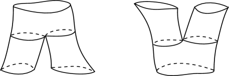
Figure 1. Elementary $2$-dimensional cobordisms.

We set

$$\partial_{\pm}\Sigma:=f^{-1}(\pm 1).$$

In the sequel, for simplicity, we will assume that $\partial_{+}\Sigma$ is connected, i.e., the pair $(\Sigma,f)$ looks like the left-hand-side of Figure 1.

We fix a Riemann metric $g$ on $\Sigma$. For simplicity we assume that in an open neighborhood $\mathcal{O}$ near $p_{0}$ there exist local coordinates such that, in these coordinates we have

$$g=dx^{2}+dy^{2},\;\;f(x,y)=-\alpha x^{2}+\beta y^{2},$$ (3.1)

where $\alpha,\beta$ are positive constants. We let $\nabla f$ denote the gradient of $f$ with respect to this metric and we set

$$C_{t}:=f^{-1}(t),\;\;t\neq 0.$$

For $t\neq 0$ we regard $C_{t}$ cooriented by the gradient $\nabla f$. Observe that $C_{t}$ has two connected components when $t<0$. We let $h_{t}:C_{t}\rightarrow{\mathbb{R}}$ be the mean curvature of this cooriented surface. For $t\neq 0$ we set

$$L_{t}=\int_{C_{t}}ds={\rm length}\,(C_{t}),\;\;\omega_{t}:=\frac{1}{4\pi}\int_{C_{t}}h_{t}ds.$$

Observe that even the singular level set $C_{0}$ is equipped with a natural measure defined by the arclength measure on $C_{0}\setminus\{0\}$. The length of $C_{0}$ is finite since in a neighborhood of the singular point $p_{0}$ the level set isometric to a pair of intersecting line segments in an Euclidean space.

Denote by $W^{\pm}$ the stable/unstable manifolds of $p_{0}$ with respect to the flow $\Phi^{t}$ generated by $-\nabla f$. The unstable manifold intersects the region $\{-1\leq f<0\}$ in two smooth paths (see Figure 2)

$$[-1,0)\ni t\mapsto a_{t},\;b_{t}\in C_{t},\;\;\forall t\in[-1,0),$$

while the stable manifold intersects the region $\{0<f\leq 1\}$ in two smooth paths (the top red arcs in Figure 2)

$$(0,1]\ni t\mapsto a_{t},\;b_{t}\in C_{t},\;\;\forall t\in(0,1].$$

Observe that $\lim_{t\rightarrow 0}a_{t}=\lim_{t\rightarrow 0}b_{t}=p_{0}$. For this reason we set $a_{0}=b_{0}=p_{0}$.

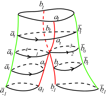
Figure 2. Cutting an elementary $2$-dimensional cobordism.

As we have mentioned before, for $t<0$ the level set $C_{t}$ consists of two curves. We denote by $C_{t}^{a}$ the component containing the point $a_{t}$ and by $C_{t}^{b}$ the component containing $b_{t}$. For $t<0$ we set

$$L_{t}^{a}:=\int_{C_{t}^{a}}ds,\;\;L_{t}^{b}:=\int_{C_{t}^{b}}ds,\;\;\omega_{t}^{a}:=\frac{1}{4\pi}\int_{C_{t}^{a}}h_{t}ds,\;\;\omega_{t}^{b}:=\frac{1}{4\pi}\int_{C_{t}^{b}}h_{t}ds$$

so that

$$L_{t}=L_{t}^{a}+L_{t}^{b},\;\;\omega_{t}=\omega_{t}^{a}+\omega_{t}^{b},\;\;\forall t<0.$$

Fix a point $\bar{a}_{-1}\in C_{-1}^{a}\setminus\{a_{-1}\}$ and a point $\bar{b}_{-1}\in C^{b}_{-1}\setminus\{b_{-1}\}$. For $t\in[-1,1]$ we denote by $\bar{a}_{t}$ (respectively $\bar{b}_{t}$) the intersection of $C_{t}$ with the negative gradient flow line through $\bar{a}_{-1}$ (respectively $\bar{b}_{t}$). We obtain in this fashion two smooth maps (see Figure 2)

$$\bar{a},\bar{b}:[-1,1]\rightarrow\Sigma.$$

For $t>0$ we denote by $I_{t}^{a}$ the component of $C_{t}\setminus\{a_{t},b_{t}\}$ that contains the point $\bar{a}_{t}$ and by $I_{t}^{b}$ the component of $C_{t}\setminus\{a_{t},b_{t}\}$ that contains the point $\bar{b}_{t}$.

The regular part $C_{0}^{*}=C_{0}\setminus\{p_{0}\}$ consists of two components $C_{0}^{a}$ and $C_{0}^{b}$. We set

$$\frac{1}{4\pi}\omega_{0}^{a}:=\frac{1}{4\pi}\int_{C_{0}^{a}}h_{0}ds,\;\;\omega_{0}^{b}:=\frac{1}{4\pi}\int_{C_{0}^{b}}h_{0}ds,\;\;\omega_{0}:=\frac{1}{4\pi}\int_{C_{0}^{*}}h_{0}ds=\omega_{0}^{a}+\omega_{0}^{b}.$$ (3.2)

Note that the limits $\lim_{t\rightarrow 0}L_{t}^{a}$, $\lim_{t\rightarrow 0}L_{t}^{b}$ exist and are finite. We denote them by $L_{0}^{a}$ and respectively $L_{0}^{b}$. We have

$$L_{0}^{a}+L_{0}^{b}=L_{0}:={\rm length}\,(C)_{0}.$$

Let $D_{t}$ denote the restriction of $\bar{\partial}$ to the cooriented curve $C_{t}$, $t\neq 0$. As explained in the previous section we have

$$D_{t}=\begin{cases}-\boldsymbol{i}\frac{d}{ds}+\frac{1}{2}h_{t},&t>0,\\ (-\boldsymbol{i}\frac{d}{ds}+\frac{1}{2}h_{t})|_{C_{t}^{a}}\oplus(-\boldsymbol{i}\frac{d}{ds}+\frac{1}{2}h_{t})|_{C_{t}^{b}}&t<0.\end{cases}$$

If we set

$$\rho_{t}=\omega_{t}-\lfloor\omega_{t}\rfloor,\;\;\rho^{a}_{t}=\omega_{t}-\lfloor\omega_{t}^{a}\rfloor,\;\;\rho^{b}_{t}=\omega_{t}-\lfloor\omega_{t}^{b}\rfloor,$$

then the computations in Section 1 imply

$$\xi(t):=\xi_{D_{t}}=\frac{1}{2}\begin{cases}1-2\rho_{t},&t>0\\ (1-2\rho^{a}_{t})+(1-2\rho^{b}_{t}),&t<0.\end{cases}$$ (3.3)

☞ Throughout this and the next section we assume that both $D_{\pm 1}$ and are invertible.

We organize the family of complex Hilbert spaces $L^{2}(C_{t},ds;{\mathbb{C}})$, $t\in[-1,1]$ as a trivial bundle of Hilbert spaces as follows.

First observe that $C_{0}\setminus\{\bar{a}_{0},\bar{b}_{0},p_{0}\}$ is a disjoint union of four open arcs $I_{1},\dotsc,I_{4}$ labeled as in Figure 2. Denote by $\ell_{j}$ the length of $I_{j}$ so that

$$L_{0}=\ell_{1}+\cdots+\ell_{4},\;\;L_{0}^{a}=\ell_{1}+\ell_{4},\;\;L_{0}^{b}=\ell_{2}+\ell_{3}.$$

For $t>0$ we can isometrically identify the oriented open arc $C_{t}\setminus\bar{a}_{t}$ with the open interval $(0,L_{t})$. We obtain in this fashion a canonical isomorphism

$$\mathcal{I}^{+}_{t}:=L^{2}(C_{t},ds;{\mathbb{C}})\rightarrow L^{2}(0,L_{t};{\mathbb{C}}).$$

The rescaling

$$(0,L_{0})\rightarrow(0,L_{t}),\;\;(0,L_{0})\ni t\mapsto\frac{t}{\lambda_{t}},\;\;\lambda_{t}=\frac{L_{0}}{L_{t}}$$

induces a Hilbert space isomorphism

$$\mathcal{R}^{+}_{t}:L^{2}(0,L_{t};{\mathbb{C}})\rightarrow L^{2}(0,L_{0};{\mathbb{C}})=:\boldsymbol{H}_{0}.$$

Note that we have a partition ${\mathcal{P}}_{+}$ of $[0,L_{0}]$

$$0=t_{0}<t_{1}<t_{2}<t_{3}<t_{4}=L_{0},\;\;t_{j}-t_{j-1}=\ell_{j},\;\;\forall j=1,\dotsc,4.$$ (3.4)

This defines a Hilbert space isomorphism

$$\mathcal{U}_{+}:L^{2}(0,L_{0};{\mathbb{C}})\rightarrow\bigoplus_{j=1}^{4}L^{2}(t_{j-1},t_{j};{\mathbb{C}})=\bigoplus_{j=1}^{4}L^{2}(I_{j},ds;{\mathbb{C}})=:\boldsymbol{H}_{0}.$$

For $t<0$ we have

$$L^{2}(C_{t},ds;{\mathbb{C}})=L^{2}(C_{t}^{a},ds;{\mathbb{C}})\oplus L^{2}(C_{t}^{b},ds;{\mathbb{C}}).$$

By removing the points $\bar{a}_{t}$ and $\bar{b}_{t}$ we obtain Hilbert space isomorphisms

$$L^{2}(C_{t}^{a},ds;{\mathbb{C}})\rightarrow L^{2}(0,L_{t}^{a};{\mathbb{C}}),\;\;L^{2}(C_{t}^{b},ds;{\mathbb{C}})\rightarrow L^{2}(0,L_{t}^{b};{\mathbb{C}})$$

that add up to a Hilbert space isomorphism

$$\mathcal{I}_{t}^{-}:L^{2}(C_{t},ds;{\mathbb{C}})\rightarrow L^{2}(0,L_{t}^{a};{\mathbb{C}})\oplus L^{2}(0,L_{t}^{b};{\mathbb{C}}).$$

By rescaling we obtain a Hilbert space isomorphism

$$\mathcal{R}^{-}_{t}:L^{2}(0,L_{t}^{a};{\mathbb{C}})\oplus L^{2}(0,L_{t}^{b};{\mathbb{C}})\rightarrow L^{2}(0,L_{0}^{a};{\mathbb{C}})\oplus L^{2}(0,L_{0}^{b};{\mathbb{C}})\cong L^{2}(0,L_{0};{\mathbb{C}}).$$

Next observe that we have isomorphisms

$$\mathcal{U}_{-}^{a}:L^{2}(0,L_{0}^{a};{\mathbb{C}})\rightarrow L^{2}(I_{1},ds;{\mathbb{C}})\oplus L^{2}(I_{4},ds{\mathbb{C}}),$$

$$\mathcal{U}_{-}^{b}:L^{2}(0,L_{0}^{b};{\mathbb{C}})\cong L^{2}(I_{3},ds;{\mathbb{C}})\oplus L^{2}(I_{3},ds;{\mathbb{C}}),$$

that add up to an isomorphisms

$$\mathcal{U}_{-}:L^{2}(0,L_{0};{\mathbb{C}})\rightarrow\bigoplus_{j=1}^{4}L^{2}(I_{j},ds;{\mathbb{C}}).$$

For $t=0$ we let $\mathcal{J}_{0}$ be the natural isomorphism

$$\mathcal{J}_{0}:L^{2}(C_{0},ds;{\mathbb{C}})\rightarrow\bigoplus_{j=1}^{4}L^{2}(I_{j},ds;{\mathbb{C}})\cong\boldsymbol{H}_{0}.$$

Now define

$$\mathcal{J}_{t}:=\begin{cases}\mathcal{U}_{+}\mathcal{R}_{t}^{+}\mathcal{I}_{t}^{+},&t>0,\\ \mathcal{U}_{-}\mathcal{R}_{t}^{-}\mathcal{I}_{t}^{-},&t<0,\\ \mathcal{J}_{0},&t=0.\end{cases}$$

We use the collection of isomorphisms $\mathcal{J}_{t}$ organizes the collection $L^{2}(C_{t},ds;{\mathbb{C}})$ as a trivial Hilbert $\mathcal{H}$ bundle over $[-1,1]$.

Remark 3.1.

Let us observe that any continous function $f:\Sigma\rightarrow{\mathbb{C}}$ induces elements $f|_{C_{t}}\in L^{2}(C_{t},ds;{\mathbb{C}})$, $\forall t\in[-1,1]$ which in turn define a continuous section of the trivial Hilbert bundle $\mathcal{H}$. $\hbox to0.0pt{$\sqcap$\hss}\sqcup$

Theorem 3.2.

(a) The operators $\mathcal{D}_{t}:=\mathcal{J}_{t}D_{t}\mathcal{J}_{t}^{-1}$ converge in the gap topology as $t\rightarrow 0^{\pm}$ to Fredholm, selfadjoint operators $\mathcal{D}_{0}^{\pm}$.

(b) The eta invariants of $\mathcal{D}_{0}^{\pm}$ exist, and we set

$$\xi_{\pm}:=\frac{1}{2}\left(\dim\ker\mathcal{D}_{0}^{\pm}+\eta_{\mathcal{D}_{0}^{\pm}}(0)\,\right),$$

If $\ker\mathcal{D}_{0}^{\pm}=0$ then we have

$$i_{APS}(\bar{\partial})+\lim_{{\varepsilon}\rightarrow 0^{+}}SF\bigl{(}\,\mathcal{D}_{t};{\varepsilon}<t\leq 1\,\bigr{)}+\lim_{{\varepsilon}\rightarrow 0^{+}}SF\bigl{(}\,\mathcal{D}_{t},\;-1\leq t<-{\varepsilon}\,\bigr{)}=-(\xi_{+}-\xi_{-}).$$ (3.5)

Proof.

We set

$$\mathcal{S}_{t}:=\begin{cases}\mathcal{U}_{+}^{-1}\mathcal{D}_{t}\mathcal{U}_{+},&t>0\\ \mathcal{U}_{-}^{-1}\mathcal{D}_{t}\mathcal{U}_{-},&t<0.\end{cases}$$

To establish the convergence statements we show that the limits $\lim_{t\rightarrow 0^{\pm}}\mathcal{S}_{t}$ exist in the gap topology of the space of unbounded selfadjoint operators on $L^{2}(0,L_{0};{\mathbb{C}})$. We discuss separately the cases $\pm t>0$, corresponding to restrictions to level sets above/below the critical level set $\{f=0\}$.

A. $t>0$. We observe that

$$\operatorname{Dom}(\mathcal{S}_{t})=\Bigl{\{}u\in L^{1,2}(0,L_{0};{\mathbb{C}});\;\;u(L_{0})=u(0)\,\Bigl{\}},\;\;\mathcal{S}_{t}(u)=-\boldsymbol{i}\lambda_{t}\frac{d}{ds}+\frac{1}{2}h_{t}\bigl{(}\,s/\lambda_{t}\,\bigr{)},$$

where we recall that the constant $\lambda_{t}$ is the rescaling factor $L_{0}/L_{t}$. We set

$$A_{t}(s):=\frac{1}{\lambda_{t}}\int_{0}^{s}h_{t}\bigl{(}\,{\sigma}/\lambda_{t}\,\bigr{)}d{\sigma}$$

Using the fact that $\lambda_{t}\rightarrow 1$ and Proposition 1.3 we see that it suffices to show that $A_{t}$ is very weakly convergent in $\mathcal{A}_{L_{0}}$; see Definition $\hbox to0.0pt{$\sqcap$\hss}\sqcup$ ‣ 1.1. Thus it suffices to prove two things.

The limit $$\lim_{t\rightarrow 0^{+}}A_{t}(L_{0}) \mathbf{A_{1}}$$ exists. ()

The limits $$\lim_{t\rightarrow 0^{+}}A_{t}(s) s\in(0,L_{0}) \mathbf{A_{2}}$$ exists for almost any . ()

Proof of ($\mathbf{A_{1}}$). Observe that

$$A_{t}(L_{0})=\int_{C_{t}}h_{t}ds=\int_{C_{t}-\mathcal{O}}h_{t}ds+\int_{\mathcal{O}\cap C_{t}}h_{t}ds,$$

where $\mathcal{O}$ is the neighborhood where (3.1) holds. The intersection of $C_{t}$ with $\mathcal{O}$ is depicted in Figure 3.

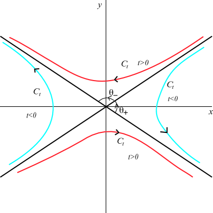
Figure 3. The behavior of $C_{t}$ near the critical point.

The integral $\int_{C_{t}\setminus\mathcal{O}}h_{t}ds$ converges as $t\rightarrow 0^{+}$ to $\int_{C_{0}\setminus\mathcal{O}}h_{0}ds$. Next observe that the intersection $C_{t}\cap\mathcal{O}$ consists of two oriented arcs (see Figure 3) and the integral $\int_{\mathcal{O}\cap C_{t}}h_{t}$ computes the total angular variation of the oriented unit tangent vector field along these oriented arcs. Using the notations in Figure 3 we see that this total variation approaches $-2\theta_{+}$ as $t\rightarrow 0+$. Hence

$$\lim_{t\rightarrow 0^{+}}A_{t}(L_{0})=\int_{C_{0}\setminus 0}h_{0}ds-2\theta_{+},$$

so that

$$\omega_{0}^{+}=\lim_{t\rightarrow 0^{+}}\omega_{t}=\frac{1}{4\pi}\lim_{t\rightarrow 0^{+}}\int_{C_{t}}h_{t}ds=\omega_{0}-\frac{\theta_{+}}{2\pi}.$$ (3.6)

Proof of ($\mathbf{A_{2}}$). Let $C_{t}^{*}:=C_{t}\setminus\{\bar{a}_{t}\}$ and define $s=s(q):C_{t}^{*}\rightarrow(0,\infty)$ to be the coordinate function on $C_{t}^{*}$ such that the resulting map

$$C_{t}^{*}\rightarrow{\mathbb{R}},\;\;q\mapsto{\sigma}(q)=s(q)/\lambda_{t}$$

is an orientation preserving isometry onto $(0,L_{t})$. In other words ${\sigma}$ is the oriented arclength function measured starting at $\bar{a}_{t}$, and $s$ defines a diffeomorphism $C_{t}^{*}\rightarrow(0,L_{0})$. Let $q_{t}:(0,L_{0})\rightarrow C_{t}^{*}$ be the inverse of this diffeomorphism.

Consider the partition (3.4). Observe that there exists positive constants $c$ and ${\varepsilon}$ such that whenever

$$\forall t\in(0,{\varepsilon}),\;\;\forall s\in[t_{1}-c,t_{1}+c]\cup[t_{3}-c,t_{3}+c]:\;\;q_{t}(s)\in\mathcal{O}$$

the numbers $t_{j}$ are defined by (3.4). Intuitively the intervals $[t_{1}-c,t_{1}+c]\cup[t_{3}-c,t_{3}+c]$ collect the parts of $C_{t}$ that are close to the critical point $p_{0}$. The length of each of the two components of $C_{t}$ that are close to $p_{0}$ is bounded from below by $2c/\lambda_{t}$.

To prove part (b) it suffices to understand the behavior of $A_{t}(s)$ for $s\in[t_{1}-c,t_{1}+c]\cup[t_{3}-c,t_{3}+c]$. We do this for one of the components since the behavior for the other component is entirely similar. We look at the component of $C_{t}\cap\mathcal{O}$ that lies in the lower half-plane in Figure 3).

Here is a geometric approach. As explained before the difference $A_{t}(s)-A_{t}(t_{1}-c)$ computes the angular variation of the unit tangent over the interval $[t_{1}-c,s]$. A close look at Figure 3 shows that the absolute value of this is bounded above by $\theta_{+}$. This proves the boundedness part of the bounded convergence. The almost everywhere convergence is also obvious in view of the above geometric interpretation. The limit function is a bounded function $A_{0}:[0,L_{0}]\rightarrow{\mathbb{R}}$ that has jumps $-\theta_{+}$ at $t_{1}$ and $t_{3}$

$$A_{0}(t_{1}^{+})-A_{0}(t_{1}^{-})=A(t_{3}^{+})-A(t_{3}^{-})=-\theta_{+},$$

while the continuous function

$$A_{0}(t)+\theta_{+}H(t-t_{1})+\theta_{+}H(t-t_{3})$$

is differentiable everywhere on $[0,L_{0}]\setminus\{t_{1},t_{3}\}$ and the derivative is the mean curvature function $h_{0}$ of $C_{0}\setminus\{p_{0}\}$.

We can now invoke Theorem 1.8 to conclude that the operators $\mathcal{D}_{t}$ converge as $t\rightarrow 0^{+}$ to the operator

$$\mathcal{D}_{0}^{+}:\operatorname{Dom}(\mathcal{D}_{0}^{+})\subset L^{2}(0,L_{0};{\mathbb{C}})\rightarrow L^{2}(0,L_{0};{\mathbb{C}}),$$

where $\operatorname{Dom}(\mathcal{D}_{0}^{+})$ consists of functions $u\in L^{2}(0,L_{0};{\mathbb{C}})$ such that

$$u|_{(t_{j-1},t_{j})}\in L^{1,2}(t_{j-1},t_{j}),\;\;\forall j=1,\dotsc,4,$$

$$u(t_{i}^{+})=e^{\boldsymbol{i}\theta_{+}/2}u(t_{i}^{-}),\;\;i=1,3,$$

$$u(t_{2}^{-})=u(t_{2}^{+}),\;\;u(t_{4}^{-})=u(t_{0}^{+}),$$

while for $u\in\operatorname{Dom}(\mathcal{D}_{0}^{+})$ we have

$$\Bigl{(}\mathcal{D}_{0}^{+}u\,\Bigr{)}|_{(t_{j-1},t_{j})}=\Bigl{(}\,-\boldsymbol{i}\frac{d}{ds}+\frac{1}{2}h_{0}(s)\,\Bigr{)}u|_{(t_{j-1},t_{j})},\;\;\forall j=1,\dotsc,4.$$

Using the point of view elaborated in Remark 1.9 we let $I$ denote the disjoint union of the intervals $I_{j}$, $j=1,\dotsc,4$. We regard $\mathcal{D}_{0}^{+}$ as a closed densely defined operator on the Hilbert space $L^{2}(I,{\mathbb{C}})$ with domain consisting of quadruples $\boldsymbol{u}=(u_{1},\dotsc,u_{4})\in L^{1,2}(I)$ satisfying the boundary condition

$$\partial_{-}\boldsymbol{u}={\boldsymbol{T}}_{+}\partial_{+}\boldsymbol{u},$$

where $\partial_{\pm}$ denotes the restriction to the outgoing/incoming boundary component of $I$, while

$${\boldsymbol{T}}_{+}:{\mathbb{C}}^{4}\cong L^{2}(\partial_{+}I)\rightarrow L^{2}(\partial_{+}I)\cong{\mathbb{C}}^{4},$$

is the transmission operator given by the unitary $4\times 4$ matrix

$${\boldsymbol{T}}_{+}=\left[\begin{array}[]{cccc}0&0&0&1\\ e^{\boldsymbol{i}\theta_{+}/2}&0&0&0\\ 0&1&0&0\\ 0&0&e^{\boldsymbol{i}\theta_{+}/2}&0\end{array}\right],\;\;\mbox{and}\;\;\mathcal{D}_{0}^{+}\left[\begin{array}[]{c}u_{1}\\ \vdots\\ u_{4}\end{array}\right]=\left(\,-\boldsymbol{i}\frac{d}{ds}+\frac{1}{2}h_{0}\,\right)\left[\begin{array}[]{c}u_{1}\\ \vdots\\ u_{4}\end{array}\right].$$

Using (1.10) we deduce that

$$\xi^{+}=\xi_{\mathcal{D}_{0}^{+}}=\frac{1}{2}(1-2\rho_{+}),\;\;\rho_{+}=\omega_{0}^{+}-\lfloor\omega_{0}^{+}\rfloor=\omega_{0}-\frac{\theta_{+}}{2\pi}-\left\lfloor\omega_{0}-\frac{\theta_{+}}{2\pi}\right\rfloor.$$ (3.7)

B. $t<0$. We observe that $\mathcal{S}_{t}=\mathcal{S}_{t}^{a}\oplus\mathcal{S}_{t}^{b}$, where for $\bullet=a,b$ we have

$$\mathcal{S}_{t}^{\bullet}:\operatorname{Dom}(\mathcal{S}_{t}^{\bullet})\subset L^{2}(0,L_{0}^{\bullet};{\mathbb{C}})\rightarrow L^{2}(0,L_{0}^{\bullet};{\mathbb{C}}),$$

$$\operatorname{Dom}(\mathcal{S}_{t}^{\bullet})=\bigl{\{}u\in L^{1,2}(0,L_{0}^{\bullet};{\mathbb{C}});\;\;u(L_{0}^{\bullet})=u(0)\,\bigr{\}},\;\;\mathcal{S}_{t}^{\bullet}u=-\boldsymbol{i}\lambda_{t}^{\bullet}\frac{d}{ds}+\frac{1}{2}h_{t}\bigl{(}\,s/\lambda_{t}^{\bullet}\,\bigr{)},$$

and $\lambda_{t}^{\bullet}$ is the rescaling factor $\frac{L_{0}^{\bullet}}{L_{t}^{\bullet}}$. It is convenient to regard $\mathcal{S}_{t}^{\bullet}$ as defined on the component $C_{0}^{\bullet}$ of $C_{0}^{*}$. Observe that $C_{0}^{a}\setminus\{\bar{a}_{0}\}=I_{1}\cup I_{4}$ and $C_{0}^{b}\setminus\{\bar{b}_{0}\}=I_{2}\cup I_{3}$. Arguing as in the case $t>0$ we conclude that

$$\lim_{t\nearrow 0}\omega_{t}^{a}=\omega_{0}^{a}+\frac{\theta_{-}}{4\pi},\;\;\lim_{t\nearrow 0}\omega_{t}^{b}=\omega_{0}^{a}+\frac{\theta_{-}}{4\pi},\;\;\omega_{0}^{-}:=\lim_{t\nearrow 0}\omega_{t}=\omega_{0}+\frac{\theta_{-}}{2\pi},$$ (3.8)

and that the operators $\mathcal{D}_{t}^{a}$ and $\mathcal{D}_{t}^{b}$ converge in the gap topology as $t\rightarrow 0^{-}$ to operators

$$\mathcal{D}_{0}^{a}:\operatorname{Dom}(\mathcal{D}_{0}^{a})\subset L^{2}(I_{1})\oplus L^{2}(I_{4})\rightarrow L^{2}(I_{1})\oplus L^{2}(I_{4}),$$

$$\mathcal{D}_{0}^{b}:\operatorname{Dom}(\mathcal{D}_{0}^{b})\subset L^{2}(I_{2})\oplus L^{2}(I_{3})\rightarrow L^{2}(I_{2})\oplus L^{2}(I_{3}),$$

where $\operatorname{Dom}(\mathcal{D}_{0}^{a})$ consists of functions $(u_{1},u_{4})\in L^{1,2}(I_{1})\oplus L^{1,2}(I_{4})$ such that

$$u_{4}(\partial_{-}I_{4})=e^{-\boldsymbol{i}\theta_{-}/2}u_{1}(\partial_{+}I_{1}),\;\;u_{4}(\partial_{+}I_{4})=u_{1}(\partial_{-}I_{1}),$$

$\operatorname{Dom}(\mathcal{D}_{0}^{b})$ consists of functions $(u_{2},u_{3})\in L^{1,2}(I_{3})\oplus L^{1,2}(I_{3})$ such that

$$u_{2}(\partial_{-}I_{2})=e^{-\boldsymbol{i}\theta_{-}/4\pi}u_{3}(\partial_{+}I_{3}),\;\;u_{2}(\partial_{+}I_{2})=u_{1}(\partial_{-}I_{3}),$$

where $\theta_{-}$ is depicted in Figure 3, and

$$\mathcal{D}_{0}^{a}(u_{1},u_{4})=\bigl{(}\,-\boldsymbol{i}\frac{du_{1}}{ds}+\frac{1}{2}h_{0}u_{1},-\boldsymbol{i}\frac{du_{4}}{ds}+\frac{1}{2}h_{0}u_{4}\,\bigr{)},$$

$$\mathcal{D}_{0}^{a}(u_{2},u_{3})=\bigl{(}\,-\boldsymbol{i}\frac{du_{2}}{ds}+\frac{1}{2}h_{0}u_{2},-\boldsymbol{i}\frac{du_{3}}{ds}+\frac{1}{2}h_{0}u_{3}\,\bigr{)}.$$

The direct sum $\mathcal{D}_{0}^{-}=\mathcal{D}_{0}^{a}\oplus\mathcal{D}_{0}^{b}$ is the closed densely defined linear operator on $L^{2}(I)$ with domain of quadruples $\boldsymbol{u}=(u_{1},\dotsc,u_{4})\in L^{1,2}(I,{\mathbb{C}})$ satisfying the boundary condition

$$\partial_{-}\boldsymbol{u}={\boldsymbol{T}}_{-}\partial_{+}\boldsymbol{u},$$

where

$${\boldsymbol{T}}_{-}:{\mathbb{C}}^{4}\cong L^{2}(\partial_{+}I)\rightarrow L^{2}(\partial_{+}I)\cong{\mathbb{C}}^{4},$$

is the transmission operator given by the unitary $4\times 4$ matrix

$${\boldsymbol{T}}_{-}=\left[\begin{array}[]{cccc}0&0&0&1\\ 0&0&e^{-\boldsymbol{i}\theta_{-}/2}&0\\ 0&1&0&0\\ e^{-\boldsymbol{i}\theta_{-}/2}&0&0&0\end{array}\right],\;\;\mbox{and}\;\;\mathcal{D}_{0}^{-}\left[\begin{array}[]{c}u_{1}\\ \vdots\\ u_{4}\end{array}\right]=\left(\,-\boldsymbol{i}\frac{d}{ds}+\frac{1}{2}h_{0}\,\right)\left[\begin{array}[]{c}u_{1}\\ \vdots\\ u_{4}\end{array}\right].$$

Then

$$\xi_{-}=\xi_{-}^{a}+\xi_{-}^{b},$$

where for $\bullet=a,b$ we have

$$\xi_{-}^{\bullet}=\frac{1}{2}(1-2\rho_{-}^{\bullet}),\;\;\rho_{-}^{\bullet}=\omega_{0}^{\bullet}+\frac{\theta_{-}}{4\pi}-\left\lfloor\,\omega_{0}^{\bullet}+\frac{\theta_{-}}{4\pi}\,\right\rfloor.$$ (3.9)

Combining (3.6) and (3.8) with the equality $\theta_{+}+\theta_{-}=\pi$ we deduce

$$\omega_{0}^{+}-\omega_{0}^{-}=\lim_{t\searrow 0}\omega_{t}-\lim_{t\nearrow 0}\omega_{t}=-\frac{1}{2}.$$ (3.10)

To prove (3.5) we use the index formula (2.8). We have

$$i_{APS}(\bar{\partial})=-\frac{1}{2}-\omega_{1}+\omega_{-1}-\xi_{D_{1}}+\xi_{D_{-1}}.$$

$$\stackrel{{\scriptstyle(\ref{eq: limit})}}{{=}}\omega_{0}^{+}-\omega_{0}^{-}-\omega_{1}+\omega_{-1}-\xi_{D_{1}}+\xi_{D_{-1}}$$

$$=(\omega_{0}^{+}+\xi^{+})-(\omega_{1}+\xi_{D_{1}})-(\omega_{0}^{-}+\xi^{-})+(\omega_{-1}+\xi_{D_{-1}})-(\xi^{+}-\xi^{-})$$

$$\stackrel{{\scriptstyle(\ref{eq: sf-xi})}}{{=}}-\lim_{{\varepsilon}\rightarrow 0^{+}}SF\bigl{(}\,\mathcal{D}_{t};{\varepsilon}<t\leq 1\,\bigr{)}-\lim_{{\varepsilon}\rightarrow 0^{+}}SF\bigl{(}\,\mathcal{D}_{t},\;-1\leq t<-{\varepsilon}\,\bigr{)}-(\xi_{+}-\xi_{-}).$$

$\hbox to0.0pt{$\sqcap$\hss}\sqcup$

Remark 3.3 (Twisted Dolbeault operators).

(a) Here the outline of an analytic argument proving ($\mathbf{A_{2}}$). Using (3.1) we deduce that this component has a parametrization compatible with the orientation given by

$$y_{t}=-\left(\zeta_{t}+mx^{2}\right)^{1/2},\;\;|x|<d_{t}$$ (3.11)

where $\zeta_{t}=\frac{t}{\beta}$, $m=\frac{\alpha}{\beta}$ and $d_{t}$ is such that the length of this arc is $2c/\lambda_{t}$. Observe that there exists $d_{*}>0$ such that $\lim_{t\rightarrow 0^{+}}dt=d_{*}$. We have

$$dy_{t}=-mx\left(\zeta_{t}+mx^{2}\right)^{-1/2}dx.$$

Set

$$y_{t}^{\prime}:=\frac{dy_{t}}{dx}=-mx\left(\zeta_{t}+mx^{2}\right)^{-1/2},$$

$$y_{t}^{\prime\prime}:=\frac{d^{2}y_{t}}{dx^{2}}=-m\left(\zeta_{t}+mx^{2}\right)^{-1/2}+m^{2}x^{2}\left(\zeta_{t}+mx^{2}\right)^{-3/2}=-\frac{m\zeta_{t}}{(\zeta_{t}+mx^{2})^{3/2}}.$$

The arclength is

$$d{\sigma}^{2}=\Bigr{(}1+(y_{t}^{\prime})^{2}\,\Bigl{)}dx^{2}=\underbrace{\left(\,1+\frac{m^{2}x^{2}}{\zeta_{t}+mx^{2}}\,\right)}_{=:w(t,x)^{2}}dx^{2}.$$

The mean curvature $h_{t}$ is found using the Frenet formulæ. More precisely $h_{t}(x)=\frac{y_{t}^{\prime\prime}}{w^{3}}$. Then

$$h_{t}d{\sigma}=h_{t}wdx=\frac{y_{t}^{\prime\prime}}{1+(y_{t}^{\prime})^{2}}dx=-\frac{m\zeta_{t}dx}{(\zeta_{t}+mx^{2})^{1/2}(\zeta_{t}+mx^{2}+m^{2}x^{2})}.$$

We observe now that we can write $h_{t}d{\sigma}=\phi_{t}^{*}(\,\rho_{\infty}du\,)$, where $\phi_{t}$ is the rescaling map

$$x\mapsto u=t^{-1/2}x\;\;\mbox{and}\;\;\rho_{\infty}(u)=-\frac{m\zeta_{1}}{(\zeta_{1}+mu^{2})^{1/2}(\zeta_{1}+mu^{2}+m^{2}u^{2})}.$$

This then allows us to conclude via a standard argument that the densities $h_{t}d{\sigma}$ converge very weakly as $t\rightarrow 0^{+}$ to a $\delta$-measure concentrated at the origin.

(b) The results in Theorem 3.5 extend without difficulty to Dolbeault operators twisted by line bundles. More precisely, given a Hermitian line bundle $L$ and a hermitian connection $A$ on $L$, we can form a Dolbeault operator $\bar{\partial}_{A}:C^{\infty}(L)\rightarrow C^{\infty}(L\otimes K^{-1}_{\Sigma})$. Fortunately, all the line bundles on a the two-dimensional cobordism $\Sigma$ are trivializable. We fix a trivialization so that the connection $A$ can be identified with a purely imaginary $1$-form

$$A=\boldsymbol{i}a,\;\;a\in\Omega^{1}(\Sigma).$$

Then

$$\bar{\partial}_{A}=\bar{\partial}+\boldsymbol{i}a^{0,1}.$$

The restriction of $D^{+}_{A}=\sqrt{2}\bar{\partial}_{A}$ to the cooriented curve $C_{t}$ is

$$D_{A}(t)=-\boldsymbol{i}\nabla^{A}_{s}+\frac{1}{2}h_{t}=-\boldsymbol{i}\frac{d}{ds}+\frac{1}{2}h_{t}+a_{t},\;\;a_{t}:=a\Bigl{(}\,\frac{d}{ds}\,\Bigr{)}\in\Omega^{0}(C_{t}).$$

As in the proof of Theorem 3.5, we only need to understand the behavior of $a_{t}$ in the neighborhood $\mathcal{O}\cap C_{t}$. Suppose for simplicity $t>0$ and we concentrate only on the component of $C_{t}\cap\mathcal{O}$ that lies in the lower half-plane of Figure 3. In the neighborhood $\mathcal{O}$ we can write

$$a=pdx+qdy,\;\;p,q\in C^{\infty}(\mathcal{O}).$$

Using the parametrization (3.11) we deduce that

$$a|_{C_{t}\cap\mathcal{O}}=\Bigl{(}\,p-mqx(\zeta_{t}+mx^{2})^{-1/2}\,\Bigr{)}dx=a_{t}ds=a_{t}wdx$$

Hence, as $t\rightarrow 0^{+}$, the measure $a_{t}ds$ converges to the measure $\bigl{(}\,p-m^{1/2}(2H(x)-1\,)\,\bigr{)}dx$

(c) One may ask what happens in the case of a cobordism corresponding to a local min/max of a Morse function. In this case $\Sigma$ is a disk, the regular level sets $C_{t}$ are circles and the singular level set is a point. Consider for example the case of a local minimum. Assume that the metric near the minimum $p_{0}$ is Euclidean, and in some Euclidean coordinates near $p_{0}$ we have $f=x^{2}+y^{2}$. Then $C_{t}$ is the Euclidean circle of radius $t^{1/2}$, and the function $h_{t}$ is the constant function $h_{t}=t^{-1/2}$. Then $\omega_{t}=\frac{1}{2}$, $\xi_{t}=\frac{1}{2}$ and the Atiyah-Patodi-Singer index of $\bar{\partial}$ on the Euclidean disk of radius $t^{1/2}$ is $0$. The operator $D_{t}$ can be identified with the operator

$$-\boldsymbol{i}\frac{d}{ds}+\frac{1}{2t^{1/2}}$$

with periodic boundary conditions on the interval $[0,2\pi t^{1/2}]$. Using the rescaling trick in Remark $\hbox to0.0pt{$\sqcap$\hss}\sqcup$ ‣ 1.6 we see that this operator is conjugate to the operator $L_{t}=-t^{1/2}\boldsymbol{i}\frac{d}{ds}+\frac{1}{2}$ on the interval $[0,2\pi]$ with periodic boundary conditions. The switched graphs of these operators

$$\widetilde{\Gamma}_{L_{t}}=\bigl{\{}(L_{t}u,u);\;\;u\in L^{1,2}(0,2\pi;\,{\mathbb{C}});\;\;u(0)=u(2\pi)\,\bigr{\}}\subset\boldsymbol{H}\oplus\boldsymbol{H},\;\;\boldsymbol{H}=L^{2}(0,2\pi;\,{\mathbb{C}}),$$

converge in the gap topology to the subspace $\boldsymbol{H}_{+}=\boldsymbol{H}\oplus 0\subset\boldsymbol{H}\oplus\boldsymbol{H}$. This limit is not the switched graph of any operator. However, this limiting space forms a Fredholm pair with $\boldsymbol{H}_{-}=0\oplus\boldsymbol{H}$ and invoking the results in [5] we conclude that the limit

$$\lim_{{\varepsilon}\searrow 0}SF(L_{t};\;\;{\varepsilon}\leq t\leq t_{0})$$

exists an it is finite. $\hbox to0.0pt{$\sqcap$\hss}\sqcup$

4. The Kashiwara-Wall index

In this final section we would like to identify the correction term in the right hand side of (3.5) with a symplectic invariant that often appears in surgery formulæ. To this aim, we need to elaborate on the symplectic point of view first outlined in Remark 1.9.

Fix a finite dimensional complex hermitian space $\boldsymbol{E}$, let $n:=\dim\boldsymbol{E}$, and set

$$\widehat{\boldsymbol{E}}:=\boldsymbol{E}\oplus\boldsymbol{E},\;\;\boldsymbol{E}_{+}:=\boldsymbol{E}\oplus 0,\;\;\boldsymbol{E}_{-}:=0\oplus\boldsymbol{E},$$

and let $J:\widehat{\boldsymbol{E}}\rightarrow\widehat{\boldsymbol{E}}$ be the unitary operator given by the block decomposition

$$J=\left[\begin{array}[]{cc}-\boldsymbol{i}&0\\ 0&\boldsymbol{i}\end{array}\right].$$

We let $\mathrm{Lag}$ denote the space of hermitian lagrangians on $\widehat{\boldsymbol{E}}$, i.e., complex subspaces $L\subset\widehat{\boldsymbol{E}}$ such that $L^{\perp}=JL$. As explained in [5, 14] any such a lagragian can be identified with the graph of a complex isometry $T:\boldsymbol{E}_{+}\rightarrow\boldsymbol{E}_{-}$, or equivalently, with the group $U(\boldsymbol{E})$ of unitary operators on $E$. In other words, the graph map

$$\Gamma:U(\boldsymbol{E})\rightarrow\mathrm{Lag}(\widehat{\boldsymbol{E}}),\;\;U(\boldsymbol{E})\mapsto\Gamma_{T}\subset\widehat{\boldsymbol{E}}$$

is a diffeomorphism. The involution $L\leftrightarrow JL$ on $\mathrm{Lag}$ corresponds via this diffeomorphism to the involution $T\leftrightarrow-T$ on $U(\boldsymbol{E})$.

We define a branch of the logarithm $\log:{\mathbb{C}}^{*}\rightarrow{\mathbb{C}}$ by requiring $\operatorname{\mathbf{Im}}\log\in[-\pi,\pi)$. Equivalently,

$$\log z=\int_{\gamma_{z}}\frac{d\zeta}{\zeta},$$

where $\gamma_{z}:[0,1]\rightarrow{\mathbb{C}}$ is any smooth path from $1$ to $z$ such that

$$\forall t\in[0,1),\;\;\gamma_{z}(t)\not\in(-\infty,0].$$

In particular, $\log(-1)=\pi\boldsymbol{i}$. Following [11, §6] we define

$$\tau:U(\boldsymbol{E})\times U(\boldsymbol{E})\rightarrow{\mathbb{R}},\;\;\tau(T_{0},T_{1})=\frac{1}{2\pi\boldsymbol{i}}\operatorname{{\rm tr}}\log(T_{1}^{-1}T_{0})$$

$$=\frac{1}{2\pi\boldsymbol{i}}\sum_{\lambda\in{\mathbb{C}}^{*}}\bigl{(}\,\log\lambda\,\bigr{)}m_{\lambda},\;\;m_{\lambda}:=\dim\ker(\lambda-T_{1}^{-1}T_{0}).$$

Observe that

$$e^{2\pi\boldsymbol{i}\tau(T_{0},T_{1})}=\frac{\det T_{0}}{\det T_{1}}$$ (4.1)

Note that

$$\tau(T_{0},T_{1})+\tau(T_{1},T_{0})=\dim\ker(T_{0}+T_{1}).$$ (4.2)

Via the graph diffeomorphism we obtain a map

$$\mu=\tau\circ\Gamma:\mathrm{Lag}\times\mathrm{Lag}\rightarrow{\mathbb{R}}.$$

The equality (4.2) can be rewritten as

$$\tau(L_{0},L_{1})+\tau(L_{1},L_{0})=\dim(L_{0}\cap JL_{1})=\dim(JL_{0}\cap L_{1}).$$ (4.3)

We want to relate the invariant $\tau$ to the eta invariant of a natural selfadjoint operator. We associate to each pair $L_{0},L_{1}\in\mathrm{Lag}$ the selfadjoint operator

$$D_{L_{0},L_{1}}:V(L_{0},L_{1})\subset L^{2}(I,\widehat{\boldsymbol{E}})\rightarrow L^{2}(I,\widehat{\boldsymbol{E}}),$$

where

$$V(L_{0},L_{1})=\bigl{\{}u\in L^{1,2}(I,\widehat{\boldsymbol{E}});\;\;u(0)\in L_{0},\;\;u(1)\in L_{1}\,\bigr{\}},\;\;D_{L_{0},L_{1}}u=J\frac{du}{dt}.$$

This is a selfadjoint operator with compact resolvent. We want to describe its spectrum, and in particular, prove that it has a well defined eta invariant. Let $T_{0},T_{1}:\boldsymbol{E}_{+}\rightarrow\boldsymbol{E}_{-}$ denote the isometries associated to $L_{0}$ and respectively $T_{1}$. Then $T_{1}^{-1}T_{0}$ is a unitary operator on $\boldsymbol{E}_{+}$ so its spectrum consists of complex numbers of norm $1$.

Proposition 4.1.

For any $L_{0},L_{1}\in\mathrm{Lag}$ we have

$$\operatorname{spec}D_{L_{0},L_{1}}=\frac{1}{2\boldsymbol{i}}\exp^{-1}\Bigl{(}\,\operatorname{spec}(T_{1}^{-1}T_{0})\,\Bigr{)}.$$ (4.4)

In particular, the spectrum of $D_{L_{0},L_{1}}$ consists of finitely many arithmetic progressions with ratio $\pi$ so that the eta invariant of $D_{L_{0},L_{1}}$ is well defined.

Proof.

Observe first that any $u\in L^{2}(I,\widehat{\boldsymbol{E}})$ decomposes as a pair

$$u=(u_{+},u_{-}),\;\;u_{\pm}\in L^{2}(I,\boldsymbol{E}_{\pm}).$$

If $u\in V(L_{0},L_{1})$ is an eigenvector of $D_{L_{0},L_{1}}$ corresponding to an eigenvalue $\lambda$ then $u$ satisfies the boundary value problems

$$-\boldsymbol{i}\frac{du_{+}}{dt}=\lambda u_{+},\;\;\boldsymbol{i}\frac{du}{dt}=\lambda u_{-},$$ (4.5a)

$$u_{-}(0)=T_{0}u_{+}(0),\;\;u_{-}(1)=T_{1}u_{+}(1).$$ (4.5b)

The equalities (4.5a) imply that

$$u_{+}(1)=e^{\boldsymbol{i}\lambda}u_{+}(0),\;\;u_{-}(1)=e^{-\boldsymbol{i}\lambda}u_{-}(0).$$

Using (4.5b) we deduce

$$e^{\boldsymbol{i}\lambda}T_{1}u_{+}(0)=u_{-}(1)=e^{-\boldsymbol{i}\lambda}u_{-}(0)=e^{-\boldsymbol{i}\lambda}T_{0}u_{+}(0).$$

Hence

$$e^{2\boldsymbol{i}\lambda}\in\operatorname{spec}(T_{1}^{-1}T_{0})\Longrightarrow\lambda\in\frac{1}{2\boldsymbol{i}}\exp^{-1}\Bigl{(}\,\operatorname{spec}(T_{1}^{-1}T_{0})\,\Bigr{)}.$$

Running the above argument in reverse we deduce that any $\lambda\in\frac{1}{2\boldsymbol{i}}\exp^{-1}\Bigl{(}\,\operatorname{spec}(T_{1}^{-1}T_{0})\,\Bigr{)}$ is an eigenvalue of $D_{L_{0},L_{1}}$. $\hbox to0.0pt{$\sqcap$\hss}\sqcup$

We let $\xi(L_{0},L_{1})$ denote the reduced eta invariant of $D_{L_{0},L_{1}}$,

$$\xi(L_{0},L_{1})=\frac{1}{2}\Bigl{(}\,\dim\ker D_{L_{0},L_{1}}+\eta_{D_{L_{0},L_{1}}}(0)\,\Bigr{)}.$$

If $e^{\boldsymbol{i}\theta_{1}},\dotsc,e^{\boldsymbol{i}\theta_{n}}$, $\theta_{1},\dotsc,\theta_{n}\in(0,2\pi]$, are the eigenvalues of $T_{1}^{-1}T_{0}$, then the spectrum of $D_{L_{0},L_{1}}$ is

$$\operatorname{spec}\bigl{(}\,D(L_{0},L_{1})\,\bigr{)}=\bigcup_{k=1}^{n}\Bigl{\{}\frac{\theta_{k}}{2}+\pi{\mathbb{Z}}\Bigr{\}}.$$

and we deduce as in Section 1 using (1.8) that

$$\eta_{D_{L_{0},L_{1}}}=\sum_{\theta_{k}\in(0,2\pi)}\Bigl{(}1-\frac{\theta_{k}}{\pi}\,\Bigr{)},$$

and

$$\xi(L_{0},L_{1})=\frac{1}{2}\sum_{\theta_{k}\in(0,2\pi)}\Bigl{(}1-\frac{\theta_{k}}{\pi}\,\Bigr{)}+\frac{1}{2}\dim\ker D_{L_{0},L_{1}}.$$

On the other hand

$$\frac{1}{2\pi\boldsymbol{i}}\operatorname{{\rm tr}}\log(-T_{1}^{-1}T_{0})=\frac{1}{2\pi}\sum_{\theta_{k}\in(0,2\pi]}(\theta_{k}-\pi)=-\frac{1}{2}\sum_{\theta_{k}\in(0,2\pi)}\Bigl{(}1-\frac{\theta_{k}}{\pi}\,\Bigr{)}+\frac{1}{2}\dim\ker(T_{0}-T_{1}).$$

Since $\ker D_{L_{0},L_{1}}\cong\ker(T_{0}-T_{1})\cong L_{0}\cap L_{1}$ we conclude

$$\tau(T_{0},-T_{1})=\tau(-T_{0},T_{1})=\tau(JL_{0},L_{1})=-\xi(L_{0},L_{1})+\dim(L_{0}\cap L_{1}).$$

Using (4.2) we deduce

$$\xi(L_{0},L_{1})=\tau(T_{1},-T_{0})=\tau(L_{1},JL_{0})=\tau(JL_{1},L_{0}).$$ (4.6)

Following [11] (see also [4]) we associate to each triplet of lagrangians $L_{0},L_{1},L_{2}$ the quantity

$$\omega(L_{0},L_{1},L_{2}):=\tau(L_{1},L_{0})+\tau(L_{2},L_{1})+\tau(L_{0},L_{2}),$$

and we will refer to its as the (hermitian) Kashiwara-Wall index (or simply the index) of the triplet. Observe that $\omega$ is indeed an integer since (4.1) implies that

$$e^{2\pi\boldsymbol{i}\omega(L_{0},L_{1},L_{2})}=1.$$

We set

$$d(L_{0},L_{1},L_{2}):=\dim(JL_{0}\cap L_{1})+\dim(JL_{1}\cap L_{1})+\dim(JL_{2}\cap L_{0}).$$

Using (4.3) we deduce that for any permutation ${\varphi}$ of $\{0,1,2\}$ with signature ${\epsilon}({\varphi})\in\{\pm 1\}$ we have

$$\omega(L_{0},L_{1},L_{2})-{\epsilon}({\varphi})\omega(L_{{\varphi}(0)},L_{{\varphi}(1)},L_{{\varphi}(2)})=d(L_{0},L_{1},L_{2})\times\begin{cases}0,&\mbox{${\varphi}$ even}\\ 1,&\mbox{${\varphi}$ odd}.\end{cases}$$ (4.7)

We want to apply the above facts to a special choice of $\widehat{\boldsymbol{E}}$. Let $\boldsymbol{I}$ denote the disjoint union of the intervals $I_{1},\dotsc,I_{4}$ introduced in Section 3. They were obtained by removing the points $\bar{a}_{0}$, $p_{0}$ and $\bar{b}_{0}$ from the critical level set $C_{0}$; Figure 2. We interpret $\boldsymbol{I}$ as an oriented $1$-dimensional with boundary and we let

$$\widehat{\boldsymbol{E}}:=L^{2}(\partial\boldsymbol{I}),\;\;\boldsymbol{E}_{\pm}=L^{2}(\partial_{\pm}\boldsymbol{I}).$$

The spaces $\boldsymbol{E}_{\pm}$ have canonical bases and thus we can identify both of them with the standard Hermitian space $\boldsymbol{E}={\mathbb{C}}^{4}$. Define $J:\widehat{\boldsymbol{E}}\rightarrow\widehat{\boldsymbol{E}}$ as before. We have a canonical differential operator

$$D_{0}:C^{\infty}(\boldsymbol{I},{\mathbb{C}})\rightarrow C^{\infty}(\boldsymbol{I},{\mathbb{C}}),\;\;D_{0}\left[\begin{array}[]{c}u_{1}\\ \vdots\\ u_{4}\end{array}\right]=\left[\begin{array}[]{c}-\boldsymbol{i}\frac{du_{1}}{dt}+\frac{1}{2}h_{0}|_{I_{1}}\\ \vdots\\ \vdots\\ -\boldsymbol{i}\frac{du_{1}}{dt}+\frac{1}{2}h_{0}|_{I_{4}}\end{array}\right],$$

We set

$$\omega_{k}:=\frac{1}{4\pi}\int_{I_{k}}h_{0}ds$$

so that

$$\omega_{0}=\omega_{1}+\cdots+\omega_{4},\;\;\omega_{0}^{a}=\omega_{1}+\omega_{4},\;\;\omega_{0}^{b}=\omega_{2}+\omega_{3}.$$

We have a natural restriction map

$$r:C^{\infty}(\boldsymbol{I},{\mathbb{C}})\rightarrow L^{2}(\partial\boldsymbol{I},{\mathbb{C}})=\widehat{\boldsymbol{E}}$$

and we define the Cauchy data space of $D_{0}$ to be the subspace

$$\Lambda_{0}:=r(\ker D_{0})\subset\widehat{\boldsymbol{E}}.$$

We can verify easily that $\Lambda_{0}$ is a Lagrangian subspace of $\widehat{\boldsymbol{E}}$ that is described by the isometry ${\boldsymbol{T}}_{0}:\boldsymbol{E}_{+}\rightarrow\boldsymbol{E}_{-}$ given by the diagonal matrix

$${\boldsymbol{T}}_{0}=\operatorname{Diag}\bigl{(}\,e^{2\pi\boldsymbol{i}\omega_{1}},\dotsc,e^{2\pi\boldsymbol{i}\omega_{4}}\,\bigr{)}.$$

☞ In the remainder of this section we assume that the operators $\mathcal{D}_{0}^{\pm}$ that appear in Theorem 3.5 are invertible.

Proposition 4.2.

Let $\mathcal{D}_{0}^{\pm}$ be the operators that appear in Theorem 3.5. Then

$$\xi_{\mathcal{D}_{0}^{\pm}}=-\xi\bigl{(}\,\Gamma_{{\boldsymbol{T}}_{\pm}},\Lambda_{0}\,\bigr{)}=\xi\bigl{(}\,\Lambda_{0},\Gamma_{{\boldsymbol{T}}_{\pm}}\,\bigr{)}=\tau(\Gamma_{{\boldsymbol{T}}_{\pm}},J\Lambda_{0})$$ (4.8)

Proof.

We need to find the spectra of ${\boldsymbol{T}}_{0}^{-1}{\boldsymbol{T}}_{\pm}$. We set $z_{k}=e^{-2\pi\boldsymbol{i}\omega_{k}}$, $k=1,\dotsc,4$ and $\rho=e^{-\boldsymbol{i}\theta_{+}/2}$, so that $e^{\-\boldsymbol{i}\theta_{-}/2}=-\boldsymbol{i}\rho$. Then

$${\boldsymbol{T}}_{0}^{*}{\boldsymbol{T}}_{+}=\left[\begin{array}[]{cccc}0&0&0&z_{1}\\ z_{2}\rho&0&0&0\\ 0&z_{3}&0&0\\ 0&0&z_{4}\rho&0\end{array}\right],\;\;{\boldsymbol{T}}_{0}^{*}{\boldsymbol{T}}_{-}=\left[\begin{array}[]{cccc}0&0&0&z_{1}\\ 0&0&-\boldsymbol{i}z_{2}\rho&0\\ 0&z_{3}&0&0\\ -\boldsymbol{i}z_{4}\rho&0&0&0\end{array}\right].$$

The eigenvalues of ${\boldsymbol{T}}_{0}^{*}{\boldsymbol{T}}_{+}$ are the fourth order roots of

$$\zeta=\rho^{2}z_{1}\cdots z_{4}=e^{\boldsymbol{i}(\theta_{+}-2\pi\omega_{0})}.$$

Hence

$$\exp^{-1}\bigl{(}\,\operatorname{spec}({\boldsymbol{T}}_{0}^{*}{\boldsymbol{T}}_{+})\,\bigr{)}=\frac{\boldsymbol{i}(\theta_{+}-2\pi\omega_{0})}{4}+\frac{\pi\boldsymbol{i}}{2}{\mathbb{Z}}$$

and using (4.4) we deduce

$$\operatorname{spec}\bigl{(}\,D_{\Gamma_{{\boldsymbol{T}}_{+}},\Lambda_{0}}\,\bigr{)}=\frac{\pi}{2}\Bigl{\{}\,\Bigl{(}\frac{\theta_{+}}{2\pi}-\omega_{0}\,\Bigr{)}+{\mathbb{Z}}\,\Bigr{\}}.$$

The eigenvalues of ${\boldsymbol{T}}_{0}^{*}{\boldsymbol{T}}_{-}$ are the square roots of

$$z_{1}z_{4}e^{\boldsymbol{i}\theta_{-}/2}=e^{-\boldsymbol{i}(\theta_{-}/2+2\pi\omega_{0}^{a})}\;\;\mbox{and}\;\;z_{1}z_{4}e^{\boldsymbol{i}\theta_{-}/2}-e^{-\boldsymbol{i}(\theta_{-}/2+2\pi\omega_{0}^{b})}.$$

Hence

$$\operatorname{spec}\bigl{(}\,D_{\Gamma_{{\boldsymbol{T}}_{+}},\Lambda_{0}}\,\bigr{)}=\left\{-\pi\left(\frac{\theta_{-}}{4\pi}+\omega_{0}^{a}\right)+\pi{\mathbb{Z}}\,\right\}\cup\,\left\{-\pi\left(\,\frac{\theta_{-}}{4\pi}+\omega_{0}^{b}\,\right)+\pi{\mathbb{Z}}\,\right\}.$$

The desired conclusion follows using (3.7), (3.9) and (1.8). $\hbox to0.0pt{$\sqcap$\hss}\sqcup$

Theorem 4.3.

Under the same assumptions and notations as in Theorem 3.5 we have

$$i_{APS}(\bar{\partial})+\lim_{{\varepsilon}\rightarrow 0^{+}}SF\bigl{(}\mathcal{D}_{t};{\varepsilon}<t\leq 1\bigr{)}+\lim_{{\varepsilon}\rightarrow 0^{+}}SF\bigl{(}\mathcal{D}_{t},\;-1\leq t<-{\varepsilon}\bigr{)}=-\omega(J\Lambda_{0},\Gamma_{{\boldsymbol{T}}_{+}},\Gamma_{{\boldsymbol{T}}_{-}}).$$

Proof.

We have

$$i_{APS}(\bar{\partial})+\lim_{{\varepsilon}\rightarrow 0^{+}}SF\bigl{(}\mathcal{D}_{t};{\varepsilon}<t\leq 1\bigr{)}+\lim_{{\varepsilon}\rightarrow 0^{+}}SF\bigl{(}\mathcal{D}_{t},\;-1\leq t<-{\varepsilon}\bigr{)}\stackrel{{\scriptstyle(\ref{eq: main})}}{{=}}-(\xi_{+}-\xi_{-})$$

$$\stackrel{{\scriptstyle(\ref{eq: eta-kashi})}}{{=}}-\tau(\Gamma_{{\boldsymbol{T}}_{+}},\Lambda_{0})-\tau(J\Lambda_{0},\Gamma_{{\boldsymbol{T}}_{-}})=-\omega(J\Lambda_{0},\Gamma_{{\boldsymbol{T}}_{+}},\Gamma_{{\boldsymbol{T}}_{-}})+\tau(\Gamma_{{\boldsymbol{T}}_{+}},\Gamma_{{\boldsymbol{T}}_{-}}).$$

To compute $\tau(\Gamma_{{\boldsymbol{T}}_{+}},\Gamma_{{\boldsymbol{T}}_{-}})=\tau({\boldsymbol{T}}_{+},{\boldsymbol{T}}_{-})$ we need to compute the spectrum of ${\boldsymbol{T}}_{-}^{*}{\boldsymbol{T}}_{+}$. We set $\rho=e^{\boldsymbol{i}\theta_{+}/2}$ so that $e^{-\boldsymbol{i}\theta_{-}/2}=-\boldsymbol{i}\rho$. We have

$${\boldsymbol{T}}_{-}^{*}{\boldsymbol{T}}_{+}=\left[\begin{array}[]{cccc}0&0&0&\boldsymbol{i}\bar{\rho}\\ 0&0&1&0\\ 0&\boldsymbol{i}\bar{\rho}&0&0\\ 1&0&0&0\end{array}\right]\,\cdot\,\left[\begin{array}[]{cccc}0&0&0&1\\ \rho&0&0&0\\ 0&1&0&0\\ 0&0&\rho&0\end{array}\right]=\left[\begin{array}[]{cccc}0&0&\boldsymbol{i}&0\\ 0&1&0&0\\ \boldsymbol{i}&0&0&0\\ 0&0&0&1\end{array}\right]$$

From the second and forth column we see that $1$ is an eigenvalue of ${\boldsymbol{T}}_{-}^{*}{\boldsymbol{T}}_{+}$ with multiplicity $2$. The other two eigenvalues are $\pm\boldsymbol{i}$, namely the eigenvalues of the $2\times 2$ minor

$$\left[\begin{array}[]{cc}0&\boldsymbol{i}\\ \boldsymbol{i}&0\end{array}\right].$$

This shows that $\tau({\boldsymbol{T}}_{+},{\boldsymbol{T}}_{-})=0$. $\hbox to0.0pt{$\sqcap$\hss}\sqcup$

Let $I$ denote the unit interval $[0,1]$. We set $\partial_{+}I=\{1\}$, $\partial_{-}I=\{0\}$. We identify $\widehat{\boldsymbol{E}}$ with the finite dimensional Hilbert space $L^{2}(\partial I,\boldsymbol{E})$ and the Hilbert spaces $\boldsymbol{E}_{\pm}$ with

References

[1] V.I. Arnold: The complex lagrangian grassmannian, Funct. Anal. and its Appl., 34(2000), 208-210.
[2] M.F. Atiyah, V.K. Patodi, I.M. Singer: Spectral asymmetry and Riemannian geometry. III, Math. Proc. Camb. Phil. Soc. 79(1976), 71-99.
[3] N. Berline, E.Getzler, M. Vergne: Heat Kernels and Dirac Operators, Springer Verlag, 1992.
[4] S. Cappell, R. Lee, E.Y. Miller: On the Maslov index, Comm. Pure Appl. Math. 47(1994), 121-186.
[5] D.F. Cibotaru: Localization formulæ in odd -theory, arXiv: 0901.2563.
[6] R. E. Edwards: Functional analysis, Dover Publications, 1995.
[7] G.B. Folland: Real Analysis. Modern Techniques and Their Applications, 2nd Edition, John Wiley & Sons, 1999.
[8] P.B. Gilkey: On the index of geometrical operators for Riemannian manifolds with boundary, Adv. Math., 102(1993), 129-183.
[9] G. Grubb: Heat operator trace expansions and index for general Atiyah-Patodi-Singer boundary problems, Comm. Partial Differential Equations, 17(1992), no.11-12, 2031-2077.
[10] T. Kato: Perturbation Theory for Linear Operators, Springer Verlag, 1995.
[11] P. Kirk, M. Lesch: The -invariant, Maslov index, and spectral flow for Dirac-type operators on manifolds with boundary, Forum Math., 16(2004), 553-629.
[12] P. Kronheimer, T. Mrowka: Monopoles and Three-Manifolds, Cambridge University Press, 2007.