Long-term photometry and periods for 261 nearby pulsating M giants

Abstract

We present the results of a 5.5-year CCD photometric campaign that monitored 261 bright, southern, semi-regular variables with relatively precise Hipparcos parallaxes. The data are supplemented with independent photoelectric observations of 34 of the brightest stars, including 11 that were not part of the CCD survey, and a previously unpublished long time-series of VZ Cam. Pulsation periods and amplitudes are established for 247 of these stars, the majority of which have not been determined before. All M giants with sufficient observations for period determination are found to be variable, with 87% of the sample (at S/N $\geq 7.5$) exhibiting multi-periodic behaviour. The period ratios of local SRVs are in excellent agreement with those in the Large Magellanic Cloud. Apparent $K$-band magnitudes are extracted from multiple NIR catalogues and analysed to determine the most reliable values. We review the effects of interstellar and circumstellar extinction and calculate absolute $K$-band magnitudes using revised Hipparcos parallaxes.

1 Introduction

Photometric surveys of M giants in the Large Magellanic Cloud (LMC), Small Magellanic Cloud (SMC), and Galactic Bulge have revealed a rich variety of pulsational behaviour. Pulsating M giants are potentially important as distance indicators since they obey period-luminosity (P-L) relations. The P-L relation for Miras has been known for decades (Eggen, 1975; Robertson & Feast, 1981; Glass & Lloyd-Evans, 1981). More recent studies have shown that semi-regular variables (SRVs) also follow well-defined P-L relations. They may pulsate on the Mira sequence or in higher overtones, where they exhibit shorter periods and smaller amplitudes than the Miras (see, for example, Wood & Sebo, 1996; Bedding & Zijlstra, 1998; Wood et al., 1999; Kiss & Bedding, 2003, 2004; Ita et al., 2004; Groenewegen, 2004; Wray, Eyer & Paczyński, 2004; Soszyński et al., 2007).

Meanwhile, studies of M giants in the local solar neighbourhood have been hampered by imprecise distances and a lack of detailed, long-term observations to enable the determination of characteristic periods. Using published periods for 24 galactic Miras and SRVs having relatively precise Hipparcos parallaxes, Bedding & Zijlstra (1998) found two parallel sequences in the ($K$, $\log P$) plane, similar to those in the LMC. Further work by Knapp et al. (2003) and Yeşilyaprak & Aslan (2004) increased the sample size and found evidence for at least two sequences, but the scatter due to imprecise parallaxes made it difficult to assign stars to distinct sequences. In the most extensive study to date, Glass & van Leeuwen (2007) used revised Hipparcos parallaxes and literature periods for 64 red giants, confirming that local stars obey similar P-L sequences to those found in the Magellanic Clouds and Bulge. However, they concluded that details remain sketchy due to insufficient data, particularly for short-period stars.

Due to their complex multi-periodic behaviour, SRVs require monitoring over several years to determine their periods, particularly since many exhibit long secondary periods superposed with short-period, small-amplitude variations. Unfortunately, targets with good Hipparcos parallaxes are too bright for surveys such as ASAS (Pojmański, 1997) and NSVS (Woźniak et al., 2004).

We have constructed a wide-field, automated survey telescope optimised for precise photometry of bright local SRVs, with the dual goals of determining periods for a sufficiently large sample to enable unambiguous identification of the local sequences, and to determine the effect of metallicity on the P-L zero-point. In this paper, we describe our sample selection (Sect. 2), the selection of $K$-band magnitudes (Sect. 3), CCD instrumentation (Sect. 4), photometric pipeline and supplementary information (Sect. 5), and PEP photometry (Sect. 6). The main result of the survey is presented in Sect. 7, where we provide periods and $K$-band magnitudes, and discuss variability, multi-periodicity, and period ratios. We summarise our results in Section 8. A detailed analysis of the results will be described in a follow-up paper, hereafter Paper II.

2 Sample Selection

Our sample of nearby variable M giants was extracted from the Hipparcos catalogue (Perryman et al., 1997), using the following criteria:

1. $\sigma_{\pi}/\pi\leq 0.2$. Catalogue entries with negative parallaxes were ignored.

2. Coarse variability flag (H6) $\geq 2$, indicating that the Hipparcos mission had observed amplitudes $\geq 0.06$ mag. This was used to select true variables.

3. Spectral type (H76) = ’M*’.

This yielded a complete sample of variable M giants to 20% parallax precision. A subsequent check prior to publication revealed that two stars (HIP 56518 & 85302) had been erroneously omitted from the sample.

The candidates were further filtered to select those likely to yield high-quality photometry:

1. Stars with declination $>35$° were removed to ensure that all candidates would transit at altitude $\geq 20$° at the observing site.

2. Stars fainter than $m_{V}=8.0$ at maximum light were excluded, retaining only those bright enough to yield photometry at the 1% level.

3. 33 stars listed in the General Catalogue of Variable Stars (GCVS) as having established periods $>100$ d were removed in order to concentrate on those undergoing short-period, low-amplitude pulsation.

This selection yielded 183 candidates. A further 67 stars with $\sigma_{\pi}/\pi<0.26$ were added to increase the total number to 250, to provide sufficient targets for a 5-hour nightly observing run. Stars were evenly distributed in right ascension so that a similar number of fields would be observed each night, regardless of the season.

In hindsight, the declination-based selection criterion was too loose, resulting in the selection of a few stars with northern declinations that were only visible for short intervals each year and so have insufficient observations to determine their periods. In addition, one star near the south celestial pole (NSV 18694) was unobservable due to a physical obstruction near the observatory.

Since our original sample selection, van Leeuwen (2007) has published revised Hipparcos parallaxes based on a re-reduction of the original data using an improved understanding of the rotation rates of the spacecraft (van Leeuwen & Fantino, 2005). The version published on VizieR on 15 September 2008, which corrected an error that affected earlier versions of the catalogue, has been used for the analysis in this paper. The original and revised distributions of the relative parallax uncertainties of our sample are shown in Figure 1. The revised distribution clearly shows an improvement for the majority of stars, with the median error reduced from 17.5% to 10.6%, consistent with the finding of Glass & van Leeuwen (2007) that parallaxes for M giants were generally improved by a factor of 2. We have adopted the revised parallaxes for our analysis.

Our CCD data are supplemented by the following sources:

1. Twenty-three stars were observed concurrently by one of us (T.T.M.) using photoelectric photometry (PEP), as described in Section 6. An additional 11 stars were observed exclusively by PEP, including 4 stars of spectral type C, one S, and one K-giant ($\lambda$ Vel).

2. VZ Cam is a northern star with a relatively precise parallax measurement (4%). We include a previously unpublished light curve obtained by B.Sz. at Konkoly Observatory.

Note that OO Aps was initially observed by PEP only, but was later added to the CCD target list to check for the possible existence of short-period pulsations.

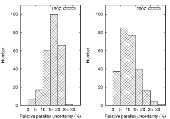
Figure 1: Distributions of relative uncertainty in parallax for the 250 M giant sample, using the original (1997) and revised (2007) Hipparcos catalogues, binned into 5% intervals.

3 $K$-band magnitudes

In preparation for a Period-Luminosity (P-L) analysis (Paper II), we obtained apparent K magnitudes as follows.

3.1 2MASS

2MASS (Cutri et al., 2003) has been the catalogue of choice for previous studies of pulsating red giants in the LMC, SMC, and Bulge. However, most of our M giants were saturated and have large uncertainties of 0.2–0.3 mag. Moreover, 2MASS magnitudes were derived from single-epoch measurements, leading to some variability-induced scatter, given that measured SRVs have $K$-band peak-to-peak amplitudes between 0.1 and 0.25 mag (Smith et al., 2004). Thus, we only used 2MASS magnitudes when better values could not be found.

3.2 The Gezari et al. Catalogue

173 M giants in our sample appear in the Catalogue of Infrared Observations (Gezari et al., 1999). All magnitudes and colour magnitudes (flags M and C, respectively) observed at a wavelength of $2.2\pm 0.05\mu$m were combined to calculate a mean $m_{K}$ for each star, weighted equally because the catalogue did not provide measurement uncertainties.

Of the 80 stars with more than one catalogued magnitude, the mean scatter (excluding seven outliers) was $0.04\pm 0.02$ mag. Seven stars had an abnormally large scatter. In two, this was caused by an apparent transcription error where the sign of the magnitude had been reversed ($\mu$ Gem and DM Eri). In other cases, a single discordant value, though not obviously wrong, was sufficiently different to yield a large scatter. As a precaution, mean magnitudes with $\sigma>0.1$ mag were not used.

3.3 DIRBE

During its 10-month cryogenic mission, DIRBE collected 100–1900 measurements for each of nearly 12000 objects (Smith et al., 2004). This permitted an accurate determination of mean $K$ magnitudes for short-period SRVs ($\sigma_{m_{K}}<$ 0.06 mag). Furthermore, DIRBE was less prone to saturation than 2MASS.

However, DIRBE had poor angular resolution due to its large beam width of 0.7°, which led to confusion between nearby NIR sources, particularly near the galactic plane ($|b|<5$°). A search of the catalogue identified matches for 222 project stars, but only 166 were marked as unconfused sources. In 5 cases, quoted errors exceeded that of 2MASS (due to insufficient observations) and were thus excluded. Following Whitelock et al. (2008), we adopt a value of 630 Jy for $m_{K}=0$, which is in good agreement with Bessell & Brett (1988).

Figure 2 compares DIRBE $K$-band magnitudes with the mean $m_{K}$ values derived from the Gezari catalogue, excluding stars marked as confused in DIRBE and those stars extracted from Gezari with $\sigma>0.1$ mag. The agreement is excellent, with a mean difference of $-0.004\pm 0.081$ mag for the 125 stars on the plot, confirming that the calibration is appropriate. The small scatter is an indication of the consistency between the homogeneous DIRBE measurements and the mean values derived from multiple measurements taken from a set of inhomogeneous catalogues. Hence, it appears safe to use Gezari magnitudes when DIRBE values are unavailable or confused with other sources.

Figure 3 compares DIRBE magnitudes with 2MASS. The larger scatter than in Figure 2 is due to the saturation-induced errors in 2MASS magnitudes. The scatter for stars marked with confusion flag 3 (001) is no worse than that for unconfused sources (000), so we retained both. However, stars with flags 1 or 2 typically show an excess in the DIRBE measurement due to contamination with a nearby source, and have been excluded.

In summary, DIRBE $K$-band magnitudes were adopted except in cases where confusion flag 1 or 2 was set, or the DIRBE uncertainty exceeded that of 2MASS. In those cases, Gezari mean magnitudes were used when available (41 stars), otherwise the 2MASS magnitude was used (25 stars).

Figure 2: Apparent $K$-band magnitudes of unconfused DIRBE sources compared to mean Gezari magnitudes, excluding stars from the latter with rms scatter $>0.1$ mag, showing an excellent correlation.

Figure 3: DIRBE vs. 2MASS $K$-band magnitudes using different symbols to denote various combinations of DIRBE confusion flags. The scatter is larger due to saturation in 2MASS.

3.4 Interstellar Extinction

Since all stars in the sample are nearby, with the most distant being PS Hya (552 pc), we expect a relatively small amount of interstellar extinction, particularly in the $K$-band. Using a $(B-V)$ vs. $(V-I)$ colour-colour diagram, we found that the majority of stars are unreddened. The maximum colour excess of $E(B-V)\sim 0.2$ occurred for 7 stars with $V-I>3.5$, implying a visual extinction of $A_{V}\sim 0.6$ mag. This was confirmed using two independent interstellar extinction models (Hakkila et al. 1997 and Drimmel, Cabrera-Lavers & López-Corredoira 2003), which indicated a maximum of $A_{V}\sim 0.5$ mag for all stars, with $A_{V}<0.2$ mag for the majority. Calculating $K$-band extinction from $A_{K}/A_{V}=0.112$ (Rieke & Lebofsky, 1985; Schlegel et al., 1998), we find an upper limit of $\sim 0.05$ mag with $A_{K}<0.02$ mag for 90% of the sample. Thus the correction is small, particularly since $M_{K}$ errors are dominated by much larger parallax uncertainties. Nevertheless, for the sake of completeness and to avoid systematic errors, corrections were applied using the model of Drimmel, Cabrera-Lavers & López-Corredoira (2003), due to its superior resolution.

3.5 Circumstellar Extinction

Small-amplitude SRVs have smaller circumstellar envelopes than their high-amplitude, more evolved counterparts, the Miras. To investigate the possibility of reddening due to a dusty envelope, we tested for IR excesses at $12\mu m$ by plotting $V-I$ vs $V-[12]$ for the 231 stars in the sample having $12\mu m$ flux densities listed in the DIRBE catalogue. Only a few stars showed a small excess. A catalogue of low-resolution spectra obtained by the Infrared Astronomical Satellite (IRAS) confirmed that 8 stars had a small amount of circumstellar dust, while 15 showed silicate emission features. Using the relation of Knapp et al. (2003, Equ 3) to estimate the $K$-band extinction caused by silicate dust, we found negligible amounts for the majority of stars ($A_{K}<0.02$ mag), and thus we have ignored the effects of circumstellar extinction.

4 CCD Observations

4.1 Equipment

An automated photometric telescope was constructed from relatively low-cost commercial components. A Nikon 80–200-mm $f$/2.8 ED telephoto lens ($D$=77 mm) coupled to an SBIG ST8-XE CCD detector with 9 $\mu$m pixels was attached to a Losmandy G-11 German Equatorial Mount controlled by an Astrometric Instruments SkyWalker II stepper motor system (Figure 4).

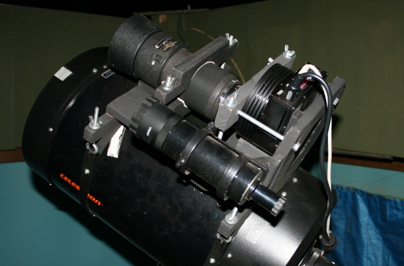
Figure 4: Survey equipment: Nikon 80–200-mm telephoto lens and SBIG ST8XE CCD detector attached to the telescope with a wooden cradle.

The telescope was housed in a roll-off roof observatory in a suburban backyard in Canberra, Australia, at latitude 35°S. Observations were gathered on nearly every clear night over a 5.5-year period using a fully automated software pipeline that controlled target selection and scheduling, telescope slewing, closed-loop pointing corrections, and camera operations (V. Tabur, PhD thesis, in prep.). In addition to the photometric survey described here, the observatory has also been used to discover a comet and two novae (Tabur et al., 2002; Tabur & Monard, 2003a; Tabur et al., 2003b).

4.2 Detector Calibration

The detector bias, readout noise and gain were determined experimentally and found to be in close agreement with the manufacturer’s stated values.

We used the procedure outlined by Berry & Burnell (2000) to determine that our detector was linear below 47000 ADU to within 0.1%. Stars with pixel values exceeding this limit (prior to calibration) were marked as saturated and were discarded by our photometric pipeline. Integrations shorter than 2 s were found to be non-linear due to a 0.02 s delay in closing the mechanical vane shutter. A shutter mapping correction was derived using the method of Zissell (2000) but was found to be unnecessary in practice because integrations longer than 3 s were used, to reduce scintillation noise.

4.3 Reducing Flux

Three methods were employed to avoid detector saturation. By stopping-down the effective aperture of the lens to $50\leq D\leq 64$ mm (during different phases of the survey) we reduced the number of photons reaching the detector. Secondly, short integration times of 3 s $\leq t_{\rm int}\leq 25$ s were employed, with the minimum practical limit set by scintillation noise and shutter effects. Broad-band photometric filters were not used because the SBIG CFW10 filter wheel does not provide sufficient back-focus when used in conjunction with a camera-lens adaptor. The unfiltered detector response is shown in Figure 5 and, for comparison, the relative transmission of a Johnson $V$-band filter, and the spectral energy distribution of a star of type M3III (Pickles, 1998).

The third way to reduce saturation was to distribute the flux over a large number of pixels. Stellar images were broadened by defocusing the optics, which also helped to improve precision by reducing sensitivity to the gate structure of the front-illuminated CCD. However, defocusing produced a complex PSF due to the multi-element optical design, and caused some blending in crowded fields, making it difficult to find isolated comparison stars and requiring more complicated analysis.

Figure 5: Quantum efficiency of the KAF1602 CCD sensor, relative transmission of a Johnson $V$-band filter (used for PEP), and the relative flux of a star of spectral type M3III, as a function of wavelength.

4.4 Automation

Once initialised each night, the telescope operated completely autonomously, allowing a very efficient survey. The observing cycle consisted of the following tasks:

1. Target selection: In general, fields were ordered by increasing R.A. so that those about to set were observed first. Allowances were made for exclusion zones to prevent frequent meridian flips when targets were in the overlap zone (visible from both sides of the mount), and to avoid obstacles. Short slews were weighted more highly to increase the duty-cycle.

2. Open-loop slewing: A telescope pointing-model (Wallace & Tritton, 1979) was used to compensate for mechanical imperfections such as polar axis misalignment, non-orthogonality of the axes, and declination axis flexure. Pointing errors were $<$ 1 arcmin when slewing to the same side of the mount, and $<$ 3 arcmin all-sky. Slews were always completed with a final movement toward the W and S to remove backlash from the gear train.

3. Closed-loop pointing correction: Residual pointing errors were corrected using a micro-slew, with the necessary offsets determined from a 2-s, low-resolution integration. The plate solution was calculated using the Optimistic Pattern Matching algorithm (Tabur, 2007), which was specifically designed to handle wide fields of view containing thousands of stars. The additional integration helped to flush the detector of any potential Residual Bulk Image caused by near saturation of the detector (Rest et al., 2002), while the final pointing correction reduced the effects of residual flat-fielding errors (Everett & Howell, 1975).

4.5 Survey Phases

Our survey consisted of three phases (Table 1). Initially, a focal-length of $f=142$ mm was employed with integrations ranging from 1 s $\leq t_{\rm int}\leq$ 25 s, and with the image slightly defocused. The detector was operated at full resolution with sub-frames read out from the central 1/3 of the CCD. The brightest targets required short exposures of $\sim$ 1–2 s, which led to a high level of scintillation noise. Despite the short integrations, some data were saturated and had to be discarded.

Phases 2 and 3 consisted of greater levels of defocus, plus an increased focal length to offset the blending of stellar sources. The sub-frame size was enlarged to increase the probability of finding bright comparison stars, which were required for the ensemble photometry.

Phase 3 used strongly defocused images yielding Full-Width at Half-Maximum (FWHM) values up to 25 pixels. Despite the difficulties this caused during analysis, requiring blended stellar sources to be deconvolved, this approach was adopted because it permitted the use of 25-s integrations for all but the very brightest targets, thus reducing scintillation noise to $\sim$ 0.5%. Although this could have been reduced further with longer integrations, the limit was set to allow $\sim$125 fields (one visible hemisphere) to be visited within a 5-hour observing window.

Multiple consecutive integrations were obtained for each target field to measure internal precision and reduce scintillation noise. A series of 3, 5, 7, or 9 images were acquired for each field utilising 25, 12, 6, or 3 s integrations, respectively. The images were analysed separately and instrumental magnitudes combined to yield mean nightly values for all targets and their comparison stars.

Even the Phase 3 regime was insufficient to prevent the two brightest stars, $\gamma$ Cru and $\beta$ Gru, from saturating the detector when observed near the meridian, although some useful images were obtained at higher airmass. Their light curves were supplemented with PEP data (Section 6).

Table 1: Survey Phases. Observations were concluded on 2008 Nov 5.

Ph	Start Date	JD	Span	Scale	FOV	FWHM
			(days)	($\arcsec$/px)	(deg)	(px)
1	2003 May 28	2452787	731	13	1.9$\times$1.2	5
2	2005 May 28	2453518	15	10	2.2$\times$1.5	10
3	2005 Jun 12	2453533	1243	10	2.9$\times$2.0	18–25

5 CCD Photometry

5.1 Flat-Fielding

Reliable flat-field images are notoriously difficult to produce for wide fields. Twilight flats have been shown to contain gradients of 1% per degree when obtained too far from the null-point, where sky-illumination gradients are minimised (Chromey & Hasselbacher, 1996), while blank sky flats are non-uniform over $0.5\degr$ scales due to natural altitude-dependent gradients (Zhou et al., 2004).

We used a combination of approaches to solve these problems. Firstly, high S/N dome flats were acquired monthly to model the high-frequency, inter-pixel variations in detector response. Illumination gradients of $\sim$ 1% were present, despite placing a two-stage diffusing screen near the entrance pupil of the optics (Zhou et al., 2004). To remove the gradients, each dome flat was corrected to match the low-frequency variations present in a master sky-flat (created by median combining 59 images obtained on a moonless night with the telescope pointing at the zenith), modelled using a 3rd-order, 2-dimensional polynomial. Finally, since the uniformity of the master sky-flat was not assured, we used the fact that an imperfect flat-field calibration will lead to spatially dependent photometric errors to determine an illumination correction. Since we observed each field hundreds of times, on both the east and west sides of the mount, the $180\degr$ rotation of the detector that occurs after a meridian-flip was used to model the change in mean magnitude of each comparison star as a function of its spatial location on the detector, analogous to the dithering of stars across an image to build a Photometric Super Flat (see Manfroid, 1995; Boyle et al., 2003). In this way, we measured gradients in the master sky-flat of up to $\pm$ 6 mmag, which we corrected in the photometric pipeline.

5.2 Atmospheric extinction

To a second-order approximation, the true magnitude of a star, $V_{0}$, measured outside of the Earth’s atmosphere, is related to the instrumental magnitude, $V_{\rm inst}$, by

$$V_{0}=V_{\rm inst}-k^{\prime}X-k^{\prime\prime}XC,$$ (1)

where $X$ is the airmass, $C$ is the colour-index of the star and $k^{\prime}$ and $k^{\prime\prime}$ are the first- and second-order extinction coefficients. By using long-term observations of the comparison stars gathered over a wide range of airmasses, we determined mean values for $k^{\prime}$ and $k^{\prime\prime}$ to be 0.16 mag airmass^-1 and 0.024 mag per airmass per unit colour, respectively. We applied the correction in the pipeline. A $V-I$ colour index was used for the colour term, to match the wide spectral response of the unfiltered detector, which spans 450 nm at FWHM and extends to the $I$ band where M giants radiate much of their energy.

5.3 Photometric precision

Magnitudes of targets and comparison stars were determined using aperture photometry. Faint, defocused stars in the sky-annulus of some comparison stars, particularly at low galactic latitudes, caused a systematic increase in sky-background measurements during bright moonlit periods, when they became difficult to separate from the real sky-background using a sigma-clipping routine. The problem was solved by mapping the positions of these stars and excluding their pixels from the sky annulus.

The photometric precision, measured as the rms scatter, is shown in Figure 6 for 4979 comparison stars. Our target stars have instrumental magnitudes brighter than 9, so they all fall in the more precise tail of the distribution. The best photometric precision achieved is limited to $\sim$ 6 mmag, even for the very brightest stars, which indicates the scintillation noise due to the small aperture and short integration times. Young (1967) described the well-known relation for atmospheric scintillation, $S$, the ratio of rms intensity fluctuation to mean intensity, as

$$S=0.09d^{-2/3}X^{3/2}\exp(-h/8000)/\sqrt{2t_{\rm int}},$$ (2)

where $d$ is the telescope aperture in cm, $X$ is the airmass, $h$ is altitude of the observing site in metres, and $t_{\rm int}$ is the integration time in seconds. Substituting values of $d$ = 6.4 cm, $h$ = 641 m, and $t_{\rm int}$ = 3 $\times$ 25 s for observations conducted during Phase 3, and assuming a mean airmass of $X$=1.5, we estimate the contribution due to scintillation to be $\sim 7$ mmag, which agrees well with the lower limit on the measured precision.

5.4 Ensemble photometry

Up to 50 of the brightest comparison stars in each field were combined to form an ensemble. We assumed constancy of the ensemble average, that is,

$$\frac{\sum{m_{i}w_{i}}}{\sum{w_{i}}}+ZP=0,$$ (3)

where $m_{i}$ are the instrumental magnitudes of the comparison stars, $w_{i}$ are their weights, and $ZP$ is the zero-point of each image in the time-series. The ensemble was used to determine iteratively the $ZP$ for each image (Balona, 1995), permitting the scatter of each comparison star to be determined, unstable stars to be excluded, and weights to be assigned to the remainder. Following Gilliland et al. (1993), weights were assigned using the reciprocal of their variance, normalised to a mean weight of 1, and clipped to a maximum value of 2 to prevent bright stars with low-amplitude variability from perturbing the solution.

Aperture photometry in crowded fields was compromised by the strong defocus, which caused some blending of stellar sources. Comparison stars were generally unaffected, since they were manually selected to avoid nearby companions. In cases where some contamination was unavoidable, the stars exhibiting the largest errors were excluded from the ensemble.

Figure 7 shows the distribution of the uncertainties for our ensemble of comparison stars, which were mostly about 3–5 mmag. Since the M giants were typically the brightest stars in each field, their internal errors were small, resulting in a total uncertainty for their differential magnitude determination of 7–8 mmag.

Figure 6: Individual comparison star scatter after correction of sky background estimates in crowded fields. Each measurement is the mean of three 25 s integrations with airmass $<2.0$ (4979 stars).

Figure 7: Distribution of mean ensemble uncertainty for 243 survey fields using 1 milli-mag bins.

5.5 Optimal Image Subtraction

Nine M giant targets were blended with nearby stars and required a Difference Image Analysis technique to subtract the flux contributed by their companions, allowing the variable sources to be measured free of contamination. Following Alard & Lupton (1998), we implemented an Optimal Image Subtraction (OIS) pipeline. High S/N images taken under the best seeing conditions were selected as reference images. Due to a small, spatially dependent asymmetry in the defocused PSF, two reference frames were selected for each field, corresponding to pre- and post-meridian-flip orientations. A high-order 2D polynomial was used to register each image with its reference to cater for the presence of optical distortions caused by the fast ($f$/2.8) optics. Well-focused images yielded residuals of $\sim$0.05 pix, but the Phase 3 images had larger residuals ($\sim$0.15 pix), due to the difficulty in determining accurate centroids for the defocused PSFs.

Since our survey fields were not crowded, we followed Kochanski et al. (1996) by only using the pixels associated with the 50 brightest stars, to prevent the Poisson noise of the blank sky background from contributing to the kernel solution. Since the tuning of OIS parameters is not straightforward, we adopted the method and recommendations of Israel et al. (2007) to determine optimal values.

Figure 8: Light curve and power spectrum of NSV 20880 (HIP 83258), which was blended with a bright companion, before (top) and after processing with OIS (bottom), resulting in the removal of the 1- and 0.5 yr peaks which dominate the original power spectrum. Note the change in scale of the corrected power spectrum.

We found that our OIS pipeline greatly improved the photometry in crowded fields. The noise in the power spectra of light curves produced using OIS were reduced, as were the strengths of spurious peaks at periods of 1 and 1/2 yr (Figure 8). We used two Cepheids (AT Pup and RS Pup), located in the field of V427 Pup, as test cases. Both have well-known periods and AT Pup is strongly blended with a brighter companion. Figure 9 shows their phased light curves, and demonstrates the dramatic improvement in photometric precision when using OIS on blended objects (upper panel). In some cases OIS did not produce optimal results, such as the slight increase in scatter for RS Pup, which we attribute to sampling issues and numerical instabilities. We restricted its use to 9 blended targets.

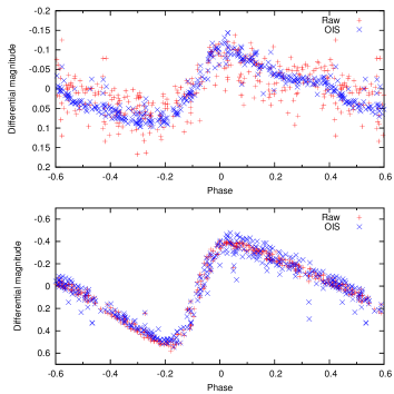
Figure 9: Phased light curves for the Cepheids AT Pup (top) and RS Pup (bottom), showing raw differential magnitudes (red pluses) and those following the application of OIS (blue crosses). AT Pup is blended with a brighter companion, leading to significant seeing-dependent aperture contamination, while RS Pup does not have a bright companion.

6 Photoelectric Photometry

Independent PEP data for 23 of the project stars were obtained by one of us (T.T.M.) as part of a survey of southern SRVs (Moon, Otero & Kiss, 2007). The PEP observations span a similar temporal range to the CCD survey, but are generally sparser due to the manual operation of the equipment. Each measurement is the mean of 5 consecutive 10-second integrations using $V$ and $B$ broadband filters, obtained in the sequence $V_{\rm star}$, $B_{\rm star}$, $B_{\rm sky}$, $V_{\rm sky}$, and bracketed by observations of two comparison stars. Measurements were corrected for extinction and transformed to standard $V$ magnitudes and $B-V$ colour indices using data from the General Catalogue of Photometric Data (Mermilliod et al. 1997).

6.1 Transformation to $V_{J}$

In order to combine CCD and PEP data, the unfiltered CCD observations of the 23 stars were transformed to Johnson $V$ magnitudes using numerous comparison stars in each field. Since some comparison stars were likely to be variable, ensembles were used to identify stable stars and their mean instrumental magnitudes. In the absence of colour information in the instrumental system, the $(V-I)_{C}$ colour index of each comparison star was used to fit the relation

$$V_{J}-V_{\rm ins}=c_{0,f}+c_{1}(V-I)+c_{2}(V-I)^{2}.$$ (4)

Here, $V_{J}$ is the Johnson $V$-band magnitude, $V_{\rm ins}$ is the mean instrumental magnitude, $c_{0,f}$ is a zero point for each field, and $c_{1}$ and $c_{2}$ are the colour terms. Separate zero-points were required for each field because the ensemble used to derive the mean instrumental magnitudes consisted of an inhomogeneous set of stars and weights.

After fitting, some stars had an excessively large difference between the catalogued $V_{J}$ and the transformed value, caused by contamination of their photometric aperture by a nearby companion, resulting in the asymmetry in Figure 10. Outliers were removed using 3 iterations of a sigma clipping routine where stars $>2.5\sigma$ from the median residual were removed. 4562 stars were retained in the final list of well-fitting, uncontaminated comparison stars, resulting in a scatter of 0.06 mag.

Figure 10: The difference between catalogued $V_{J}$ and the transformed values as a function of $V-I$ colour index. Stars with an excess are involved with a close companion that increased the measured flux within the photometric aperture, resulting in the asymmetrical distribution.

Although the fit was reasonable for the comparison stars, the cooler M giants exhibited larger residuals with systematic differences between the two systems (Figure 11, left panel). We attribute these to the lack of instrumental colour information for use in the transformation, together with the use of an unfiltered detector that was sensitive to a broad range of wavelengths, and extrapolating the relation to cool temperatures beyond the range of comparison star colour indices $(V-I>1.7)$. The left panel shows an approximately linear systematic difference between $V_{J}$ in the CCD and PEP systems for the M giants, as a function of spectral type. The filtered PEP data are approximately 0.05 mag brighter than the unfiltered CCD for M2III stars, and the difference increases to 0.37 mag for later-types. A hint of the same trend is visible in Figure 10 for $2<V-I<2.5$, corresponding to spectral types up to M2III, though there are too few stars to be certain, since most M giant comparison stars were variable and were thus excluded from the fit.

To adjust for the difference, a zero-point correction was added to align the CCD and PEP light curves. The correction was determined by using the CCD observations that bracketed each PEP observation by $\pm 2$ days to interpolate the CCD magnitude to the same date as the PEP observation. The mean difference between the CCD and PEP magnitudes defined the offset.

Figure 11 (right panel) shows the rms uncertainty of $(V_{J,\rm CCD}-V_{J,\rm PEP})$ residuals after applying the zero-point correction, as a function of spectral type. Most stars have a small scatter of $\sim$ 0.02 – 0.04 mag, somewhat larger than the uncertainty of the PEP measurements, which were generally better than 0.01 mag. We attribute the differences to errors in the transformation. However, as expected, the coolest stars exhibit a larger scatter, caused by a systematic increase in passband difference due to the transmission of longer wavelengths on the red side of the $V$-band cut-off, to which our unfiltered CCD is sensitive.

The PEP and CCD light curves exhibit the same general features, although the former exhibit greater $V$-band amplitudes (Figure 12). The most extreme example occurs for the M8III variable V744 Cen, which has a 36% greater amplitude in the PEP system. Fortunately, the coolest stars exhibit long-period, large-amplitude variations and so their periods are well determined using CCD data alone (Table 2).

Table 2: Late-type stars with large residuals after fitting a zero point to transformed CCD observations. PEP data were ignored when determining periods for these stars.

HIP	Name	Amp	Std Dev	Period	Spectral
		(mag)	(mag)	(days)	Type
61404	BO Mus	0.55	0.069	133	M6II/III
66666	V744 Cen	1.11	0.122	167	M8III
98608	$\nu$ Pav	0.45	0.066	87.8	M6III
106044	SX Pav	0.54	0.064	50.5	M5III

Figure 11: Mean difference between M-giant $V_{J}$ magnitudes in the CCD and PEP systems as a function of Morgan-Keenan spectral type (left), and the resulting $1\sigma$ scatter in the differences after applying a zero-point correction as described in the text (right). Late-type stars exhibit greater errors due to increasing differences in effective passband.

Figure 12: CCD (top panel) and PEP light curves of $\beta$ Gru. The agreement is good, with the PEP observations exhibiting a slightly larger photometric amplitude.

6.2 VZ Cam

VZ Cam was observed by one of us (B.Sz.) using the 24^′′ telescope of the Konkoly Observatory between 1968 and 1977. The data were obtained with an RCA 1P21 photomultiplier through Johnson $UBV$ filters, using two comparison stars (comp=HD 57508, $V$=6.550, $B-V$=0.966 and $U-B$=0.63; check=HD 55075, $V$=6.325, $B-V$=$-$0.040 and $U-B$=$-$0.05). The typical photometric accuracy is $\pm$0.01–0.02 mag. The star was observed in a program for obtaining long-term photometric data for the peculiar Pop. II Cepheid RU Cam (Szeidl et al., 1992). We added the object to our sample because of its accurate Hipparcos parallax and the previously unknown two periods that can be determined from the decade-long light curve. This is the first analysis of VZ Cam in the literature.

7 Period Analysis

Characteristic periods were determined for each light curve using a weighted Discrete Fourier Transform (DFT). The weighted mean magnitude of the set was first subtracted to prevent a peak at zero frequency from dominating the spectrum. Observations were weighted by the inverse square of their uncertainty, except those combined with PEP data, which were analysed using multiple weighting schemes as described below. The DFT code was an implementation of the algorithm proposed by Scargle (1989, Appendix D), modified to include weights for each point.

Observations were predominantly spaced at intervals of 1 day, resulting in a Nyquist frequency of 0.5 cycle day^-1. Power spectra were created for the frequency range 0–0.4 cycle day^-1. When searching for the most significant peak (greatest power), only frequencies $<0.2$ cycle day^-1 were considered, corresponding to a pulsation period $>$ 5 d. The mean power in the frequency range 0.2–0.4 cycle day^-1, where no pulsation signal is expected, was used to estimate the noise level. The peaks at low frequency have lower S/N because of the rising noise floor, caused by $1/f$ noise. Only periods shorter than 300 d were kept, since we consider them to be the most reliable. Longer periods were less well determined due to gaps in the sampling, possible instrumental drifts, and difficulty matching light curves in different phases due to insufficient comparison stars in the earlier, smaller FOVs.

Light curves containing both CCD and PEP data showed higher noise in their corresponding DFTs compared to those prepared using CCD data only. Noise levels were at a minimum when all observations were weighted equally, but increased for weighting schemes using $\sigma^{-1}$ and $\sigma^{-2}$. This effect was caused by the $V$-filtered PEP observations having larger amplitudes than the unfiltered CCD data (Figure 12), probably caused by the lack of instrumental colour information in the transformation. However, since the periods are well-correlated, we find that despite the increase in noise, the fitted periods remain unaffected. Since equal numbers of PEP and CCD observations tend to produce the greatest noise, the weighting scheme was selected dynamically based on the relative number of observations. An inverse variance was used when the number of CCD observations exceeded the PEP observations by a factor of two, otherwise equal weights were used.

Periods were extracted using iterative sinewave fitting (Frandsen et al., 1995). That is, least-squares minimisation was used to fit a sinusoid with a frequency corresponding to the strongest peak in the DFT, while solving for the optimum amplitude and phase. The best-fitting sinusoid was subtracted from the data, and the process repeated until no strong peaks (S/N $\geq 7.5$) remained.

7.1 The catalogue

The survey results are presented in Table LABEL:T4, with stars ordered by ascending Hipparcos catalogue number (column 1). Columns 2 and 3 list the star name, and spectral type from the Bright Star Catalogue (Hoffleit & Warren, 1991) where available, otherwise from the General Catalogue of Variable Stars (Samus et al., 2009, GCVS), or the most recent entry from the compilation of spectral types by Skiff (2009). Additional columns list the Johnson $V$-band magnitude, revised Hipparcos parallax and uncertainty (van Leeuwen, 2007), apparent $K$ magnitude, absolute $K$ magnitude and uncertainty, $K$-band magnitude source (described in Section 3; D=DIRBE, G=Gezari, 2M=2MASS), number of CCD and PEP observations, and detected periods.

GZ Eri and NSV 16260 are listed as G and K giants, respectively, although other sources list them as M giants (Houk & Smith-Moore, 1988; Houk, 1982). The shape of their light curves and the derived periods are consistent with the usual variability in early M-type stars. Fourteen stars have no determined periods, although we retain them in Table LABEL:T4 to document their $M_{K}$. Five of these stars (BW Oct, NSV 18694, V931 Her, V983 Her, and V2158 Cyg) have no observations due to physical obscuration or low altitude. A further 6 stars ($\gamma$ Hyi, $\lambda$ Vel, V1919 Cyg, V2090 Cyg, V2114 Cyg, V345 Peg) have insufficient observations for reliable period determination. The remaining 3 stars have either long periods, or periods with low S/N, both of which were excluded by our selection criteria, as follows. X Tra shows two periods of $\sim 385$ and $\sim 455$ d. CI Boo shows a long period of $\sim 485$ d and a shorter period of $\sim 51$ d, although the latter is only detected at S/N $\approx$ 7.2. V440 Aur has a possible 39 d period which is only detected at S/N $\approx$ 5.8.

7.2 Sample light curves

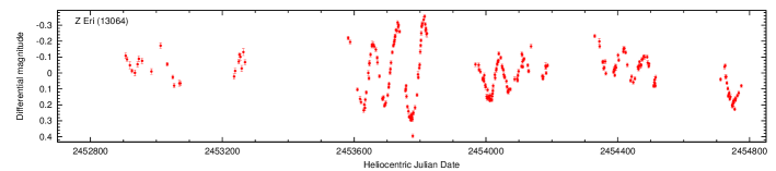
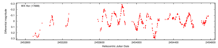
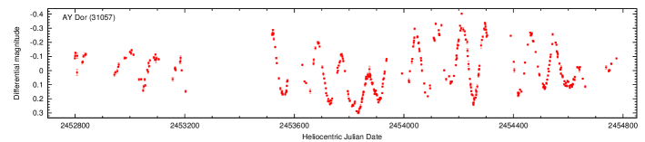
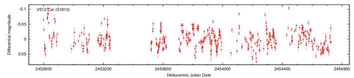
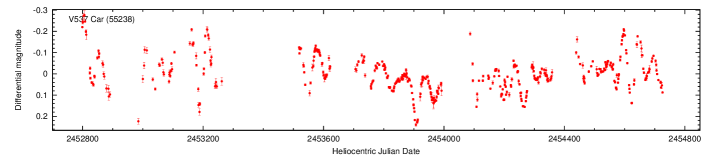
Figure 16: A selection of light curves. CCD and PEP observations are denoted by red(solid) and blue(open) points, respectively. Hipparcos catalogue numbers are listed in parentheses.

A selection of light curves and their corresponding power spectra are shown in Appendix A in the online version of the paper (see Supporting Information). Figures 16 and 17 show an example light curve and power spectrum for Z Eri. The full set of plots are available on request from the authors, and photometric data are available electronically from CDS, Strasbourg.

Relatively few stars show Mira-like light curves with regular, high-amplitude, mono-periodic behaviour, although our selection in the appendix is biased toward higher-amplitude variability for aesthetic reasons (see for example, DU Cha and AY Dor). Instead, the majority of stars exhibit short-period variability on time-scales of 10–100 d, small amplitudes ($A<$ 0.2 mag), and multiple periods, resulting in complicated light curves (see, for example, V512 Car).

It is well known that the excited frequencies in SRVs are not stable over time, and may vary by a few percent (Mattei et al., 1997; Kiss et al., 1999). The amplitudes of the modes can vary on timescales of 1–5 yr (Kiss et al., 2000; Percy et al., 2003), and in some cases, phase variations have been observed on short time-scales, consistent with the properties of a stochastically excited and damped oscillator (Bedding et al., 2005). Consequently, the complex light variations of SRVs cannot be fully modelled by a simple sum of sine waves. The occurrence of closely separated frequencies is quite common amongst our sample (see, for example, Z Eri, WX Hor, $\epsilon$ Mus, BL Cru), and is probably caused by modulations in the amplitude and/or phase of a single oscillation mode, and may indicate the finite lifetime of the oscillation. We did not try to combine periods by introducing arbitrary criteria, but instead, provide the raw data in Table LABEL:T4.

We found that 63% of periods are shorter than 50 d and nearly 5% of periods are shorter than 15 d. Of these, the shortest reliable period is 8.7 d (NSV 15560, $A=$9 mmag) and corresponds to the strongest peak in its power spectrum (see Fig A6). The shortest period belongs to NSV 18346 ($P$=6.7 d, M3III, $J-K$=1.16, $M_{K}$=$-$4.7) but has an amplitude of only 5 mmag and may be spurious.

Although we did not retain periods longer than 300 d in Table LABEL:T4, we note that WW Pic exhibits a long period of $\sim$ 370 d and a short period of 36.1 d. The period ratio of $\sim$ 10 is consistent with galactic SRVs having long secondary periods (LSP). Although the precise nature of their variations are still unknown (Oliver & Wood, 2003; Wood et al., 2004), LSP behaviour has been identified amongst SRVs in the lower metallicity environment of the LMC (Wood et al., 1999). Moreover, WW Pic has an $M_{K}$=$-$4.74, placing the 370-d period on sequence D of Wood et al. (1999), which is composed of LMC stars having LSPs.

Table 3: Survey results.

HIP	Name	Spectral	$m_{V}$	$\pi$	$m_{K}$	$M_{K}$	Src	$N_{C}$	$N_{P}$	Periods
		Type	(mag)	(mas)	(mag)	(mag)				(days)
154	YY Psc	M3III	4.37	7.55 (0.59)	$-$0.47	$-$6.09 (0.17)	D	267	0	23.1 32.0 53.6 167.8
1158	AD Cet	M3+III	5.13	5.60 (0.30)	$+$0.50	$-$5.77 (0.12)	D	272	0	18.6 29.2 212.3
1170	AE Cet	M3III	4.44	7.29 (0.28)	$+$0.20	$-$5.50 (0.08)	D	324	0	19.2 19.6 27.1 41.7
2086	HD 2268	M1III	6.24	2.07 (0.66)	$+$1.74	$-$6.69 (0.69)	G	260	0	16.8 22.7 39.1 202.0
2210	$\eta$ Scl	M4III	4.86	7.22 (0.51)	$+$0.09	$-$5.62 (0.15)	D	334	0	22.7 23.5 24.6 47.3 128.7 158.7
2215	AG Cet	M3	7.35	4.22 (0.56)	$-$0.04	$-$6.92 (0.29)	G	273	0	57.6 126.3
2219	TV Psc	M3III	5.01	6.17 (0.59)	$-$0.17	$-$6.23 (0.21)	D	207	0	55.1 216.5 266.7
3632	NSV 00293	M4III	5.36	4.20 (0.29)	$+$0.25	$-$6.65 (0.15)	D	205	0	24.3 25.7 37.3 115.2
3894	BU Phe	M4III	7.19	3.70 (0.45)	$+$2.00	$-$5.17 (0.27)	D	420	0	22.7 32.9 92.9 218.3
4200	BQ Tuc	M4III	5.73	4.58 (0.28)	$+$0.20	$-$6.50 (0.13)	D	454	138	31.6 45.0 60.9
4317	HR 259	M4III	6.19	5.75 (0.42)	$+$1.04	$-$5.18 (0.16)	D	137	0	18.8
4879	CC Tuc	M2III	6.25	3.76 (0.32)	$+$1.57	$-$5.56 (0.19)	D	425	161	16.2 20.3 20.6
6487	NSV 00490	M3III	7.05	3.40 (0.69)	$+$2.52	$-$4.83 (0.45)	D	252	0	16.4 18.3 34.6
6952	AW Phe	M2III	6.25	3.22 (0.42)	$+$1.35	$-$6.11 (0.29)	D	387	0	30.5 43.0 66.0 71.5 159.0 219.3
7505	CY Psc	M4	6.39	3.54 (0.49)	$+$1.53	$-$5.73 (0.30)	D	210	0	33.5
7506	NSV 15347	M3III	6.18	4.37 (0.32)	$+$1.41	$-$5.39 (0.16)	D	429	0	13.9 17.9 23.6 37.6 91.7
8240	HD 10934	M3III	5.49	5.14 (0.25)	$+$1.04	$-$5.41 (0.11)	D	418	0	11.8 13.8 20.0 20.2 158.7
8837	$\psi$ Phe	M4III	4.39	9.54 (0.19)	$-$0.65	$-$5.75 (0.04)	D	376	119	43.7 48.1
9171	AA Tri	M5.5	6.94	5.11 (0.46)	$+$0.17	$-$6.29 (0.20)	D	49	0	23.5
9372	AR Cet	M3III	5.43	6.85 (0.31)	$-$0.39	$-$6.21 (0.10)	D	248	0	22.0 22.9 28.7 37.3 100.7
10155	NSV 00738	M3III	5.68	5.84 (0.49)	$+$0.95	$-$5.25 (0.18)	D	123	0	18.1 21.9
11293	TZ Hor	M5III	6.39	4.33 (0.41)	$+$0.78	$-$6.05 (0.21)	D	405	131	23.3 52.9 69.8 116.7
11455	CL Hyi	M6/7	7.17	6.20 (0.45)	$+$0.03	$-$6.02 (0.16)	D	392	0	66.4 71.9 75.8 94.1 100.1
11648	TV Hor	M4-5III	6.76	3.42 (0.33)	$+$1.11	$-$6.24 (0.21)	D	424	0	32.9 33.6 34.8 47.1 69.9 248.1
12016	FH Eri	M4III	7.03	3.22 (0.51)	$+$1.65	$-$5.82 (0.35)	D	375	0	20.0 20.8 21.7 22.1 28.5 30.2 156.7
12433	NSV 15560	M3III	7.85	2.56 (0.59)	$+$3.06	$-$4.91 (0.52)	D	360	0	8.7 112.2
13064	Z Eri	M4III	6.63	3.90 (0.49)	$+$0.34	$-$6.71 (0.27)	D	253	0	75.4 80.1 123.5
13613	NSV 15611	M3III	7.38	4.25 (0.68)	$+$2.80	$-$4.06 (0.37)	D	323	0	12.2 23.5 28.5 253.8
13654	RZ Ari	M6-III	5.76	9.28 (0.30)	$-$1.03	$-$6.23 (0.07)	D	141	0	49.9 54.8
13756	EH Cet	M4III	6.15	4.42 (0.53)	$+$1.11	$-$5.69 (0.26)	D	196	0	37.2 62.5 91.6
14456	HD 19349	M3III	5.23	7.15 (0.41)	$+$0.52	$-$5.22 (0.13)	D	232	0	12.9 31.8 115.7 191.9
14930	TW Hor	C7,2(N0)	5.71	3.11 (0.37)	$+$0.09	$-$7.45 (0.26)	D	0	45	270.3
15474	$\tau^{4}$ Eri	M3.5III	3.70	10.71 (0.54)	$-$1.19	$-$6.04 (0.11)	D	284	0	23.8
16484	NSV 15716	M2III	7.92	2.45 (0.50)	$+$3.62	$-$4.45 (0.52)	2M	398	0	18.5 25.5
17678	$\gamma$ Hyi	M2III	3.26	15.24 (0.11)	$-$0.93	$-$5.02 (0.03)	D	0	16
17889	WX Hor	M5/6III	7.45	3.13 (0.54)	$+$0.67	$-$6.86 (0.38)	D	382	0	66.8 92.6 99.8 156.3 260.4
17993	GL Eri	M5III	7.05	3.24 (0.44)	$+$1.38	$-$6.08 (0.30)	D	322	0	29.6 39.6 41.8 285.7
18048	GM Eri	M4III	7.57	3.37 (0.58)	$+$1.77	$-$5.60 (0.38)	D	336	0	60.4 123.0 210.1
18605	NSV 15865	M3III	7.64	2.81 (0.43)	$+$3.15	$-$4.62 (0.37)	D	378	0	94.2 161.8
18691	XY Dor	M1III	6.51	2.61 (0.38)	$+$1.99	$-$5.92 (0.33)	D	381	0	13.3 17.1 22.9 28.9 190.8 271.7
18744	$\gamma$ Ret	M4III	4.48	6.95 (0.11)	$-$0.45	$-$6.24 (0.04)	G	383	157	30.0 42.8 277.0
18931	DP Eri	M5III	7.24	3.46 (0.66)	$+$1.64	$-$5.67 (0.42)	D	310	0	15.5 26.8 90.5 183.2
20075	GZ Eri	G8III	6.00	2.16 (0.38)	$+$0.72	$-$7.62 (0.38)	D	320	0	49.1 52.0 57.4 224.7
20856	RV Cae	M1III	6.41	2.74 (0.35)	$+$2.15	$-$5.67 (0.28)	D	334	0	25.7 34.5 37.5 117.2
20958	V1145 Tau	M3.5III	6.93	3.59 (0.60)	$+$1.58	$-$5.70 (0.37)	D	189	0	27.2 41.3 84.7
21296	DV Eri	M3III	5.20	3.28 (0.26)	$+$0.66	$-$6.79 (0.17)	D	234	0	28.9 44.2 62.2
21479	R Dor	M8III	5.59	18.31 (0.99)	$-$4.02	$-$7.71 (0.14)	D	0	72	168.9
21763	DM Eri	M4III	4.32	8.85 (0.60)	$-$0.34	$-$5.61 (0.15)	D	304	0	18.8 45.5
22667	$o^{1}$ Ori	S3.5/1-	4.71	5.01 (0.71)	$-$0.51	$-$7.02 (0.31)	D	171	0	30.8 70.7
22737	NSV 1777	M0-1III	6.43	2.73 (0.37)	$+$2.34	$-$5.48 (0.41)	2M	335	0	19.8 20.4 27.4 45.5 83.8 95.2
23653	NSV 16242	M2III	6.26	3.95 (0.35)	$+$2.03	$-$4.99 (0.21)	D	367	0	13.1 18.4 92.9 109.4
23840	WZ Dor	M3III	5.19	5.77 (0.18)	$+$0.33	$-$5.87 (0.07)	D	388	135	26.0 44.5
23874	NSV 01842	M1III	6.33	3.89 (0.45)	$+$1.74	$-$5.35 (0.26)	D	255	0	13.4 16.7 17.3 42.8
24169	RX Lep	M6III	5.60	6.71 (0.44)	$-$1.38	$-$7.26 (0.14)	D	248	0	90.1 101.7
24189	NSV 16260	K5III	6.57	2.44 (0.39)	$+$2.42	$-$5.65 (0.36)	D	298	0	15.9 22.3 30.5 66.4 90.7
24441	V1365 Ori	M3	6.89	4.10 (0.53)	$+$0.71	$-$6.24 (0.28)	D	220	0	42.3 62.7
24943	WW Pic	M3/4III	6.60	2.94 (0.39)	$+$1.92	$-$5.74 (0.29)	D	334	0	36.1 72.8 285.7
25194	SW Col	M1III	5.73	5.02 (0.37)	$+$1.14	$-$5.37 (0.16)	D	316	0	78.7 156.5
26005	NSV 16342	M2/3III	7.07	2.34 (0.53)	$+$2.59	$-$5.57 (0.50)	D	303	0	18.1 20.2 27.0 39.2 91.0
26169	WX Men	M3III	5.79	3.00 (0.31)	$+$0.60	$-$7.04 (0.23)	D	283	170	38.5 39.7 40.1 43.5 54.4 115.2
27229	WY Lep	M4/M5III	6.54	5.28 (0.47)	$+$0.59	$-$5.80 (0.19)	D	288	0	32.2 47.3 162.9 183.8
27344	NSV 16680	M5III	6.78	3.31 (0.35)	$+$1.87	$-$5.54 (0.24)	D	324	0	14.2 14.7 21.2 50.2 196.5
27661	V440 Aur	M3III	6.28	5.44 (0.72)	$+$1.17	$-$5.17 (0.29)	D	46	0
28596	SW Pic	M4III	6.41	3.40 (0.32)	$+$1.13	$-$6.22 (0.21)	D	396	123	25.1 35.5
28874	S Lep	M6III	6.74	4.92 (0.63)	$-$0.55	$-$7.10 (0.28)	D	280	0	97.3
28984	YY Lep	M4III	5.74	2.60 (0.39)	$+$0.46	$-$7.47 (0.33)	D	282	0	38.8 41.6 56.9 80.6
29048	NSV 16782	M2III	5.28	3.89 (0.33)	$+$1.03	$-$6.03 (0.19)	D	300	0	19.9 29.2 39.6 88.7 165.6
29263	AF Col	M2II-III	5.54	3.83 (0.25)	$+$0.66	$-$6.44 (0.15)	D	319	0	42.0 43.9 48.6 112.5 250.6
29353	$\eta^{2}$ Dor	M2.5III	5.01	5.09 (0.23)	$+$0.45	$-$6.03 (0.10)	D	337	46	21.4 21.8 23.3 150.2
29509	V1389 Ori	M2III	6.45	5.48 (0.51)	$+$2.12	$-$4.20 (0.22)	D	218	0	18.0 27.8 35.2
30237	AC Pic	M3III	6.79	2.61 (0.40)	$+$2.01	$-$5.91 (0.35)	D	374	0	25.8 26.2 35.0
30343	$\mu$ Gem	M3III	2.87	14.08 (0.71)	$-$1.88	$-$6.15 (0.11)	D	154	0	25.2 40.5
30352	NSV 16859	M1III	6.30	2.96 (0.29)	$+$1.90	$-$5.75 (0.22)	D	358	0	15.3 19.8
31057	AY Dor	M6II/III	7.22	3.03 (0.47)	$+$0.60	$-$6.99 (0.34)	G	369	0	78.3 86.4
31086	KM CMa	M4III	6.31	3.18 (0.41)	$+$1.57	$-$5.94 (0.28)	D	303	0	57.6 115.6 234.7
31099	SX Col	M1III	6.26	4.53 (0.31)	$+$1.50	$-$5.23 (0.16)	D	314	0	17.5 21.2 22.0 22.5 30.3 31.5 89.6
31363	V729 Mon	M2III	6.68	3.75 (0.67)	$+$1.52	$-$5.63 (0.49)	2M	227	0	23.3 33.5 47.5
32374	NSV 17193	M2III	7.18	2.61 (0.47)	$+$2.59	$-$5.32 (0.41)	D	365	0	14.6 15.7 35.7 56.0
33040	KX CMa	M4III	6.33	3.58 (0.46)	$+$0.42	$-$6.82 (0.28)	D	271	0	37.1 50.6 62.7
35120	NSV 03486	M4-III	5.78	6.01 (0.37)	$+$0.74	$-$5.37 (0.14)	G	215	0	11.9 30.2 64.7
35626	MZ CMa	M4III	5.87	5.10 (0.37)	$+$1.21	$-$5.26 (0.16)	G	296	0	15.8 17.6 18.7 23.9 25.6 34.9 49.6
35746	GH CMa	M6III	6.96	3.31 (0.67)	$+$0.84	$-$6.58 (0.44)	D	295	0	44.4 55.7 62.1 89.7
36547	VZ Cam	M4III	4.92	6.53 (0.25)	$-$0.13	$-$6.05 (0.19)	2M	0	695	27.1 28.1 38.5 39.0 54.4 205.3 249.4
36982	NSV 17548	M0III	6.72	2.69 (0.36)	$+$2.07	$-$5.78 (0.31)	D	135	0	13.2
37321	NSV 17542	M1III	7.38	2.96 (0.63)	$+$2.59	$-$5.08 (0.50)	2M	256	0	21.8 49.1 184.8
37508	NSV 17555	M2III	5.79	4.19 (0.33)	$+$1.34	$-$5.56 (0.18)	G	218	0	13.2 18.4 37.7
37521	NZ Gem	M3II-III	5.55	2.52 (0.60)	$+$0.71	$-$7.29 (0.52)	D	200	0	30.1 31.5 43.8 63.7 166.4
38406	BC CMi	M4III	6.30	6.45 (0.47)	$+$0.79	$-$5.17 (0.16)	D	230	0	27.7 143.3 208.3
38834	V341 Car	M0III	7.06	3.81 (0.40)	$+$1.29	$-$5.83 (0.23)	D	396	0	30.5 274.7
39070	V460 Car	M1.5IIa	5.19	3.32 (0.20)	$+$0.68	$-$6.74 (0.35)	2M	413	0	32.9 34.3
39299	NSV 03872	M1III	6.31	4.06 (0.51)	$+$1.38	$-$5.62 (0.36)	2M	331	0	21.2 25.4
39659	BL Cnc	M3III	5.96	4.38 (0.53)	$+$1.30	$-$5.50 (0.27)	D	176	0	22.6 37.8 203.7
40144	V427 Pup	M5	6.64	3.77 (0.34)	$+$1.00	$-$6.17 (0.34)	2M	307	0	38.7 52.5 57.4 243.3
40282	HR 3247	M1III	5.52	4.52 (0.22)	$+$2.00	$-$4.75 (0.11)	G	366	0	13.2 16.1 24.3 114.9
41080	NSV 17870	M1III	5.92	2.53 (0.59)	$+$1.41	$-$6.58 (0.51)	D	247	0	17.7 22.8 25.5 33.4 94.5 220.3
42176	NSV 17929	M0	7.36	4.66 (0.77)	$+$2.86	$-$3.81 (0.40)	D	240	0	37.9
42502	AK Hya	M4III	6.59	6.40 (0.41)	$-$0.61	$-$6.59 (0.14)	D	294	0	78.6 88.7 133.7
43215	AK Pyx	M5III	6.42	4.68 (0.41)	$+$0.57	$-$6.09 (0.19)	D	340	0	55.5 57.9 86.7 162.9 232.6
44126	FZ Cnc	M4III	6.30	5.32 (0.44)	$+$1.23	$-$5.14 (0.18)	D	210	0	17.6
44281	AL Pyx	M1III	7.19	2.70 (0.42)	$+$2.39	$-$5.48 (0.34)	G	308	0	36.1 44.5 55.3 60.0 192.3 284.1
44538	NSV 18130	M4/5III	7.78	3.55 (0.54)	$+$2.21	$-$5.06 (0.35)	D	349	0	9.5 15.2 15.6 140.1
44816	$\lambda$ Vel	K4Ib-IIa	2.23	5.99 (0.11)	$-$1.57	$-$7.68 (0.04)	D	0	26
45902	$\theta$ Pyx	M1III	4.71	6.49 (0.45)	$+$0.54	$-$5.41 (0.15)	D	338	0	13.0 98.3
45924	NSV 18181	M1III	5.56	5.68 (0.28)	$+$1.23	$-$5.01 (0.33)	2M	319	0	15.1 21.7 32.0 123.0 143.7
46027	NSV 18186	M2III	6.83	2.54 (0.54)	$+$1.73	$-$6.27 (0.47)	D	286	0	15.7 15.9 20.6 27.5 130.9
46521	AL Ant	M2/M3III	7.48	3.06 (0.65)	$+$2.39	$-$5.20 (0.47)	D	390	0	27.5 38.2 40.8 131.4 174.2
46620	V482 Car	M2III	5.88	3.37 (0.45)	$+$1.02	$-$6.36 (0.38)	2M	416	0	25.5 26.0 34.2 166.1 216.9
47608	NSV 18257	M1/2III	6.97	2.92 (0.48)	$+$2.57	$-$5.14 (0.44)	2M	396	0	8.7 11.2 14.5 19.2 67.0 97.7
49610	IO Hya	M4III	6.99	3.62 (0.72)	$+$1.40	$-$5.82 (0.43)	D	347	0	26.3 31.9 34.5 43.9 93.7 170.1
49755	PS Hya	M3III	7.09	1.59 (0.78)	$+$2.40	$-$6.62 (1.07)	D	308	0	17.4 29.6 99.2
49902	NSV 18346	M3III	6.74	4.56 (0.48)	$+$1.98	$-$4.74 (0.24)	D	332	0	6.7 8.9 141.6
49926	V368 Car	M3III	6.07	4.07 (0.30)	$+$1.05	$-$5.92 (0.30)	2M	454	0	22.6 29.4 30.0 41.6
50332	GY Vel	M4-5III	6.20	4.56 (0.33)	$+$0.42	$-$6.30 (0.16)	G	415	0	20.0 25.3 25.9 26.5 35.7 36.7 116.6
50626	V501 Car	M4III	6.96	3.33 (0.36)	$+$1.70	$-$5.70 (0.36)	2M	314	0	22.7 24.2 32.4 45.8 48.2
50827	UV Sex	M3III	7.05	3.10 (0.81)	$+$2.08	$-$5.48 (0.57)	D	305	0	34.6 36.6 48.7 83.8
51049	V347 Vel	M1III	7.00	2.79 (0.45)	$+$2.60	$-$5.21 (0.43)	2M	406	0	19.5 29.1 32.2 42.6 46.3 136.6 179.5
51141	V505 Car	M3III	6.61	3.15 (0.29)	$+$1.79	$-$5.74 (0.36)	2M	259	61	26.5
51327	NSV 18423	M1III	6.42	4.90 (0.29)	$+$1.95	$-$4.62 (0.19)	D	435	0	9.1 11.7 23.6 182.1
51810	V512 Car	M3III	6.87	2.76 (0.41)	$+$1.92	$-$5.90 (0.34)	D	423	0	25.2 34.6 35.7 50.2
51905	$\phi^{2}$ Hya	M1III	6.01	4.31 (0.33)	$+$1.87	$-$4.97 (0.18)	D	334	0	11.0 110.3 153.6
53449	VY Leo	M5.5III	5.91	8.39 (0.37)	$-$0.79	$-$6.18 (0.10)	D	236	0	35.8 54.9 75.0 84.5
54474	NSV 18694	M2III	6.87	2.76 (0.36)	$+$2.18	$-$5.65 (0.30)	D	0	0
54593	V897 Cen	M3III	7.47	3.12 (0.61)	$+$2.23	$-$5.32 (0.49)	2M	395	0	16.2 21.2 21.4 30.3 39.2 82.8
54708	V532 Car	M4III	6.24	4.12 (0.42)	$+$0.65	$-$6.29 (0.23)	D	463	0	33.7 35.3 49.6 91.0
54725	NSV 05129	M1III	6.35	3.55 (0.47)	$+$1.78	$-$5.49 (0.29)	D	389	0	15.0 153.4
54974	UU Crt	M4III	6.86	1.84 (0.49)	$+$1.58	$-$7.12 (0.58)	D	312	0	35.5 54.0 55.7 78.0 189.4 273.2
54999	SY Crt	M4III	6.51	4.09 (0.73)	$+$1.04	$-$5.92 (0.39)	D	318	0	28.6 32.4 38.7 42.5 45.6 176.4
55238	V537 Car	M6III	6.61	2.97 (0.50)	$-$0.05	$-$7.71 (0.52)	2M	461	0	39.9 51.2 52.8 71.9
56293	NSV 18788	M1III	6.15	4.54 (0.36)	$+$1.57	$-$5.15 (0.18)	D	390	0	16.7 18.3 24.6 28.5 34.9 133.0
56698	V912 Cen	M3/M4III	6.85	2.19 (0.62)	$+$1.65	$-$6.68 (0.62)	D	338	0	27.9 37.3 38.4 40.1 137.4
56702	V913 Cen	M5/7	6.56	6.08 (0.52)	$-$0.06	$-$6.15 (0.19)	G	443	0	34.0 70.6 247.5
56779	$\omega$ Vir	M4III	5.24	6.56 (0.36)	$-$0.24	$-$6.16 (0.12)	D	279	0	23.9 25.0 29.5 31.0 59.0
56970	V914 Cen	M1III	5.95	2.86 (0.52)	$+$1.67	$-$6.07 (0.48)	2M	361	0	21.8 31.1 43.6 51.6 252.5
57380	$\nu$ Vir	M1III	4.04	11.10 (0.18)	$+$0.09	$-$4.69 (0.04)	D	264	0	11.1 12.3 16.8 23.7
57411	WW Crt	M4III	7.54	3.86 (0.59)	$+$1.97	$-$5.11 (0.33)	G	399	0	16.0 17.7 23.7 26.4 50.9 83.5 123.3 133.9
57505	DU Cha	M6III	7.67	4.42 (0.39)	$+$0.34	$-$6.45 (0.19)	D	323	0	58.0 60.1
57607	V919 Cen	M7III	7.02	4.14 (0.73)	$-$1.18	$-$8.11 (0.38)	D	405	0	97.9 116.4 193.4 225.7
57613	II Hya	M4+III	5.10	5.98 (0.27)	$-$0.30	$-$6.43 (0.10)	D	381	0	29.5 30.4 39.5 41.4 89.1
57800	RU Crt	M3	8.14	7.57 (0.98)	$+$0.07	$-$5.54 (0.28)	D	328	0	60.6 66.4 101.1
59588	V335 Hya	M4III	6.34	2.79 (0.46)	$-$0.17	$-$7.96 (0.36)	D	429	0	107.6 141.2
59929	$\epsilon$ Mus	M5III	4.06	10.82 (0.17)	$-$1.43	$-$6.26 (0.03)	G	408	251	32.1 32.7 42.5 43.7 44.9 46.0 63.4 196.5
60333	KO Vir	M6	7.64	4.53 (0.65)	$+$1.71	$-$5.02 (0.31)	D	314	0	18.4 22.3 24.6 32.1 56.1 116.7 157.0
60421	TT Crv	M3III	6.48	3.53 (0.39)	$+$1.64	$-$5.64 (0.24)	D	332	0	15.4 15.6 19.5 19.9 26.8 37.7 182.8
60781	BL Cru	M4-5III	5.38	7.36 (0.32)	$-$0.19	$-$5.87 (0.10)	D	482	179	30.7 42.3 43.6
60979	V928 Cen	M2II-III	6.00	4.42 (0.37)	$+$1.16	$-$5.63 (0.19)	D	434	0	19.0 19.2 22.3 24.6 29.6 46.4 102.2
61084	$\gamma$ Cru	M3.5III	1.59	36.83 (0.18)	$-$3.10	$-$5.27 (0.06)	G	209	232	12.1 15.1 16.5 54.8 82.7 104.9
61404	BO Mus	M6II-III	6.11	2.97 (0.32)	$-$0.83	$-$8.48 (0.23)	D	488	156	134.8 229.9
61658	FW Vir	M3+III	5.68	6.62 (0.31)	$+$0.94	$-$4.96 (0.10)	D	301	0	9.3 28.6 89.7
61908	V341 Hya	M3III	6.64	4.32 (0.43)	$+$1.72	$-$5.12 (0.23)	D	415	0	8.6 18.3 18.7 36.2 216.5 281.7
62247	LM Mus	M5III	7.11	4.87 (0.47)	$+$1.40	$-$5.18 (0.32)	2M	401	0	20.8 28.9 30.0 30.5 42.4
62985	$\psi$ Vir	M3-III	4.77	5.99 (0.23)	$+$0.14	$-$5.99 (0.09)	D	348	0	22.4 23.5 24.5 30.1 31.3 49.4 162.6
63090	$\delta$ Vir	M3+III	3.39	16.44 (0.22)	$-$1.24	$-$5.16 (0.03)	D	229	0	13.0 17.2 25.6 110.1 125.8
63752	KX Vir	M4.5III	7.41	3.19 (0.71)	$+$1.76	$-$5.73 (0.49)	D	332	0	15.6 17.8 23.4 25.6 69.4 77.6 250.0
63950	FS Com	M5III	5.53	4.43 (0.41)	$-$0.20	$-$6.97 (0.20)	D	253	0	33.7 44.6 46.8 159.5
64117	NSV 06103	M1III	6.34	3.55 (0.44)	$+$1.81	$-$5.46 (0.41)	2M	313	0	14.4 16.8 25.4 183.8 250.6
64645	LO Vir	M6	7.30	3.75 (0.53)	$+$1.64	$-$5.50 (0.31)	D	332	0	20.0 22.0 22.3 26.8 91.7
64852	$\sigma$ Vir	M1III	4.78	4.83 (0.19)	$+$0.49	$-$6.10 (0.09)	D	328	0	23.4 24.3 27.9 34.1 35.8 64.0 165.3
65311	NSV 06212	M1III	6.17	3.99 (0.34)	$+$1.70	$-$5.31 (0.19)	D	440	0	17.9 21.7 22.4 22.7 31.7 34.0 52.2 99.7
66666	V744 Cen	M5III	5.74	6.35 (0.33)	$-$0.72	$-$6.72 (0.12)	D	461	75	95.8 102.2 166.9
66783	LY Mus	M4III	6.91	3.48 (0.41)	$+$0.95	$-$6.37 (0.26)	D	405	0	53.1 55.3 84.7 106.6 128.7 261.8
67288	NSV 06442	M2III	5.41	4.82 (0.39)	$+$1.01	$-$5.60 (0.18)	D	376	0	18.3 18.5 18.8 25.4 25.9 50.2
67457	V806 Cen	M4.5III	4.19	17.82 (0.21)	$-$1.67	$-$5.41 (0.03)	D	354	107	26.5
68815	$\theta$ Aps	M7III	5.69	8.84 (0.49)	$-$2.02	$-$7.29 (0.12)	D	0	259	100.9 111.0
68937	ER Vir	M4III	6.57	4.16 (0.50)	$+$1.45	$-$5.48 (0.26)	D	372	0	16.1 18.8 25.7 29.6 80.2
69269	ET Vir	M2III	4.93	7.08 (0.32)	$+$0.58	$-$5.18 (0.18)	D	367	0	22.6 23.8 36.4 37.6 39.8 48.8 259.1
69614	FS Vir	M4III	6.41	4.04 (0.52)	$+$1.54	$-$5.44 (0.28)	D	351	0	13.5 16.1 17.0 22.6 144.7 170.1
69850	NQ Aps	M3III	7.28	2.82 (0.62)	$+$1.93	$-$5.84 (0.49)	D	241	0	21.2 28.2
70236	CI Boo	M3III	6.50	4.23 (0.47)	$+$0.58	$-$6.29 (0.24)	D	141	0
72122	HD 129902	M1III	6.06	3.46 (0.51)	$+$1.78	$-$5.54 (0.32)	D	283	0	11.3 19.8 32.3 211.0
72432	V768 Cen	M3III	5.89	6.34 (0.34)	$-$0.44	$-$6.44 (0.12)	D	460	0	41.4 57.4 60.9 145.1 191.2
72655	NSV 20194	M0III	7.26	3.83 (0.67)	$+$2.37	$-$4.73 (0.38)	G	515	0	15.8 19.2 19.4 28.3 47.7 192.3
73589	EV Boo	M4III	6.60	3.08 (0.41)	$+$0.70	$-$6.86 (0.29)	G	137	0	31.2 35.3 59.3
73764	GM Lup	M6III	6.29	5.40 (0.56)	$+$0.00	$-$6.35 (0.23)	G	387	0	29.9 43.6 45.5 61.3 80.9 243.3
74582	X TrA	C5,5(Nb)	5.75	2.78 (0.44)	$-$0.62	$-$8.39 (0.34)	D	0	160
74982	FZ Lib	M4III	6.95	2.84 (1.03)	$+$1.00	$-$6.76 (0.79)	D	357	0	22.2 25.9 26.4 62.3
74999	OO Aps	M2III	6.59	2.82 (0.45)	$+$1.81	$-$5.93 (0.36)	D	67	103	24.9
76423	$\tau^{4}$ Ser	M5IIb-III	6.51	4.86 (0.46)	$-$1.02	$-$7.60 (0.21)	D	329	0	86.7 173.0 244.5
76573	LY Ser	M4III	6.82	4.75 (0.47)	$-$0.46	$-$7.09 (0.22)	D	243	0	66.7 76.5 220.8
79072	FS Ser	M3.5III	5.69	4.04 (0.43)	$+$0.56	$-$6.41 (0.23)	G	354	0	20.6 25.2 25.6 26.4 48.4
79086	FQ Ser	M4III	6.47	4.92 (0.73)	$+$0.54	$-$6.01 (0.33)	G	354	0	31.3 32.1 36.2 41.4 44.0 71.5 144.1
79349	LQ Her	M4.5III	5.74	4.78 (0.31)	$+$0.15	$-$6.46 (0.14)	D	274	0	24.5 25.1 28.0 29.9 33.6
79754	V368 Nor	M2III	5.45	4.21 (0.43)	$+$0.62	$-$6.27 (0.22)	G	396	0	18.9 21.4 22.1 24.2 33.6
80047	$\delta^{1}$ Aps	M5III	4.68	4.28 (0.16)	$-$0.73	$-$7.59 (0.08)	G	307	0	68.0 94.9 101.7
80620	V2105 Oph	M3-III	5.24	5.65 (0.39)	$+$0.48	$-$5.80 (0.15)	D	371	0	20.5 21.2 21.4 41.6 206.6
81376	V840 Ara	M2/M3III	6.84	4.67 (0.57)	$+$1.84	$-$4.83 (0.38)	2M	384	0	16.3 17.9 24.3 42.6 51.1 75.5 164.7
81426	V904 Her	M2III	6.96	2.87 (0.52)	$+$2.19	$-$5.54 (0.40)	D	224	0	22.8 65.5 95.4 257.7
82028	HR 6227	M3III	5.60	7.19 (0.42)	$+$0.82	$-$4.91 (0.13)	D	345	0	13.2 14.7 17.1 21.9 38.7
83258	NSV 20880	M4III	7.39	3.05 (0.64)	$+$1.74	$-$5.86 (0.46)	G	345	0	13.3 14.6 15.8 18.9 181.2
83462	V931 Her	M4III	6.19	4.35 (0.33)	$+$0.70	$-$6.11 (0.17)	G	0	0
84744	NSV 21509	M1III	6.80	3.42 (0.48)	$+$2.48	$-$4.86 (0.35)	D	160	0	19.3
84780	V2113 Oph	M5III	6.43	6.43 (0.52)	$-$0.21	$-$6.18 (0.18)	D	372	0	47.3 49.3 70.5 76.1 257.1
84833	V656 Her	M2III	5.01	6.80 (0.36)	$+$0.89	$-$4.96 (0.13)	D	343	0	22.3 93.9 176.1 234.7 283.3
84938	NSV 21626	M2.5III	6.35	3.26 (0.49)	$+$2.08	$-$5.37 (0.33)	D	348	0	19.7 23.6
85435	V859 Ara	M2II	7.07	3.90 (0.58)	$+$1.94	$-$5.12 (0.40)	2M	372	0	14.6 18.9 24.9 35.2 97.8 125.3
85760	NO Aps	M3III	5.83	3.69 (0.28)	$+$0.75	$-$6.44 (0.17)	D	0	207	26.2 26.6
85934	V642 Her	M4III	6.36	5.42 (0.52)	$+$0.95	$-$5.40 (0.21)	D	364	0	21.9 25.5 33.6 35.4 61.2 130.5 153.4 229.9
86153	V959 Her	M4III	6.37	4.23 (0.44)	$+$1.41	$-$5.46 (0.24)	D	188	0	25.3 35.7
87390	HD 162189	M2III	5.94	5.77 (0.56)	$+$1.80	$-$4.40 (0.21)	G	207	0	14.1 28.5
88563	V980 Her	M2III	6.97	3.39 (0.53)	$+$2.27	$-$5.10 (0.42)	2M	358	0	19.1 24.6 26.0 31.4 135.3
88761	V983 Her	M…	7.33	3.28 (0.47)	$+$2.38	$-$5.05 (0.32)	D	0	0
89172	V669 Her	M3III	4.96	5.99 (0.22)	$+$0.33	$-$5.79 (0.08)	D	152	0	22.9 24.0
89527	V2392 Oph	M4III	6.10	4.22 (0.50)	$+$0.68	$-$6.22 (0.26)	D	379	0	17.6 20.0 25.9 32.0 33.2 97.7
91135	V4401 Sgr	M4III	6.77	6.46 (0.56)	$+$0.72	$-$5.24 (0.19)	G	387	0	18.8 23.1 23.8 24.2 33.4 35.9
91789	V536 Lyr	M…	8.20	2.64 (0.71)	$+$2.11	$-$5.81 (0.59)	D	127	0	50.8 282.5
92079	V4405 Sgr	M4III	6.34	4.49 (0.40)	$+$0.42	$-$6.33 (0.19)	G	291	0	21.3 26.2 32.6 38.8 66.9
93270	V387 Vul	M3.5III	6.28	4.63 (0.41)	$+$0.81	$-$5.89 (0.21)	G	294	0	15.8 19.2
93919	NSV 24691	M1	7.53	5.45 (0.72)	$+$1.93	$-$4.40 (0.29)	G	380	0	12.0 15.5 103.2
94646	HD 180377	M2III	6.46	3.88 (0.53)	$+$1.79	$-$5.29 (0.30)	G	331	0	14.9 16.5 16.7 34.6 296.7
94969	V389 Vul	M4	6.95	4.27 (0.57)	$+$0.39	$-$6.48 (0.29)	G	307	0	36.1 49.4 58.9 82.3 226.8
96111	V4419 Sgr	M4III	6.58	4.59 (0.62)	$+$1.03	$-$5.68 (0.30)	D	414	0	29.3 39.9 57.4
96310	V1919 Cyg	M3III	6.64	3.17 (0.39)	$+$1.50	$-$6.01 (0.27)	G	15	0
96399	NSV 24813	M4/5III	6.71	4.63 (0.59)	$+$1.21	$-$5.47 (0.28)	D	460	0	11.9 12.0 13.9 15.3 21.4 29.0 135.1
97142	V2090 Cyg	M1III	6.39	3.36 (0.36)	$+$0.74	$-$6.65 (0.24)	G	11	0
97365	$\delta$ Sge	M2II+A0V	3.68	5.49 (0.72)	$-$0.78	$-$7.09 (0.28)	D	286	0	32.4 34.0 34.8 54.2
98438	VZ Sge	M4III	5.33	3.20 (0.31)	$-$0.10	$-$7.59 (0.21)	G	319	0	36.5 39.2 51.4 65.1
98500	V345 Tel	M4III	6.75	5.40 (0.59)	$+$1.50	$-$4.85 (0.24)	G	461	0	17.2 20.5 22.4 42.3 75.4
98608	NU Pav	M6III	4.95	6.86 (0.26)	$-$1.47	$-$7.29 (0.09)	D	434	112	59.0 62.0 87.0 124.7 272.5
98688	V3872 Sgr	M4III	4.43	7.27 (0.18)	$-$0.76	$-$6.46 (0.06)	D	367	0	24.0 30.4 31.3 42.8 50.5 234.7
98954	V1472 Aql	M2.5III	6.37	7.92 (1.07)	$+$1.73	$-$3.78 (0.29)	G	318	0	100.2
100051	V2114 Cyg	M5	7.23	2.50 (0.51)	$+$0.86	$-$7.18 (0.44)	G	12	0
101316	MT Del	M4II-III	7.12	3.39 (0.66)	$+$2.13	$-$5.23 (0.42)	G	307	0	26.0 29.0 50.7 64.1 103.7
101810	EU Del	M6III	6.22	8.56 (0.50)	$-$1.12	$-$6.46 (0.14)	G	265	0	44.0 60.8 67.3 132.6 235.3
102096	AV Mic	M3II	6.28	2.85 (0.40)	$+$1.10	$-$6.64 (0.31)	D	438	0	22.3 23.3 30.3 31.0 32.3 45.0 110.7
102624	EN Aqr	M3III	4.43	5.57 (0.28)	$-$0.22	$-$6.50 (0.11)	D	346	0	20.2 24.9 27.2 35.0 36.9 143.9 197.2
102720	FI Vul	M3	7.65	5.15 (0.60)	$+$0.16	$-$6.29 (0.25)	D	270	0	53.8 64.6 73.7 111.7
103645	V2142 Cyg	M3III	6.85	3.53 (0.43)	$+$2.47	$-$4.81 (0.30)	D	88	0	22.3
104755	NSV 25504	M1-2III	5.06	3.65 (0.67)	$+$0.69	$-$6.51 (0.40)	D	424	0	15.5 88.3 130.9 162.6 228.3
104974	NSV 13620	M3III	5.31	5.33 (0.33)	$+$0.54	$-$5.84 (0.14)	D	348	0	19.5 20.1 24.3 91.5
105334	T Ind	C7,2(Na)	6.15	1.72 (0.40)	$+$0.60	$-$8.22 (0.51)	D	0	51	157.5
105518	NSV 25556	M2III	7.10	2.93 (0.57)	$+$2.81	$-$4.87 (0.49)	2M	348	0	16.6
105678	Y Pav	C7,3(N0)	6.28	2.48 (0.59)	$+$0.33	$-$7.70 (0.52)	D	0	152	232.0
105846	V2158 Cyg	M…	7.77	4.18 (0.59)	$+$1.99	$-$4.92 (0.33)	D	0	0
106044	SX Pav	M5III	5.47	7.92 (0.28)	$-$0.71	$-$6.22 (0.34)	2M	422	236	36.0 50.6 53.1 77.6 88.9
106062	NV Peg	M4.5III	5.84	4.90 (0.32)	$-$0.16	$-$6.72 (0.14)	D	261	0	44.0 45.4 77.0 91.5
107516	EP Aqr	M8III	6.52	8.80 (0.63)	$-$1.53	$-$6.81 (0.16)	D	324	0	81.8 117.9 125.8
109212	OY Peg	M1	6.31	3.26 (0.38)	$+$1.62	$-$5.83 (0.26)	D	260	0	28.1 29.4 38.6 41.0 64.3 202.0
110256	BO Oct	M5III	5.09	11.22 (0.23)	$-$1.16	$-$5.92 (0.05)	D	0	315	18.0 23.1 23.4 201.6
110346	PT Peg	M4III	6.46	4.43 (0.48)	$+$1.35	$-$5.43 (0.24)	D	163	0	164.7
110364	DN Oct	M3III	7.30	2.89 (0.47)	$+$2.06	$-$5.67 (0.36)	D	232	0	17.9 32.4
110428	BW Oct	M7III	8.73	4.00 (0.66)	$-$0.27	$-$7.29 (0.36)	D	0	0
110478	$\pi^{1}$ Gru	S5	6.42	6.13 (0.76)	$-$2.15	$-$8.21 (0.27)	D	0	101	198.8
111043	$\delta^{2}$ Gru	M4.5III	4.12	9.88 (0.23)	$-$0.87	$-$5.90 (0.06)	G	370	212	20.6 24.1 24.5 32.3 33.3 97.6 125.9 205.8
111310	$\nu$ Tuc	M4III	4.91	11.24 (0.23)	$-$0.14	$-$4.89 (0.05)	D	408	210	22.3 24.4 24.8 25.1 25.5 33.8 50.6 80.1 123.2 261.8
112102	NSV 25945	M5III	6.12	4.73 (0.39)	$+$1.13	$-$5.50 (0.18)	D	371	0	13.2 15.5 17.2 27.4 106.3
112122	$\beta$ Gru	M5III	2.07	18.43 (0.42)	$-$3.21	$-$6.88 (0.05)	D	303	245	28.1 37.1 37.7 38.4 39.2 39.7 105.6 232.6
112961	$\lambda$ Aqr	M2.5III	3.73	8.47 (0.66)	$-$0.64	$-$6.01 (0.17)	D	273	0	24.5 32.0 49.5
113330	DM Tuc	M8III	7.43	4.49 (0.50)	$-$0.09	$-$6.83 (0.24)	D	430	0	137.6 153.6 170.4 208.3
113881	$\beta$ Peg	M2.5II-III	2.44	16.64 (0.15)	$-$2.21	$-$6.11 (0.07)	G	115	0	43.3
114318	Y Scl	M4	8.43	6.05 (0.81)	$+$0.39	$-$5.71 (0.30)	D	377	0	95.7 291.5
114347	GZ Peg	M4III	5.05	4.17 (0.34)	$-$0.45	$-$7.36 (0.18)	D	273	0	40.1 42.2 46.5 49.4 80.3
114404	V345 Peg	M3	6.69	4.01 (0.51)	$-$0.06	$-$7.06 (0.28)	D	8	0
114407	DL Gru	M4III	5.90	3.55 (0.43)	$+$0.74	$-$6.51 (0.26)	D	398	0	18.6 23.4 24.0 24.5 29.5 30.1 162.1
114939	$\chi$ Aqr	M3III	4.93	5.32 (0.37)	$-$0.29	$-$6.67 (0.15)	D	299	0	32.3 38.5 44.9
115433	DR Tuc	M3III	6.08	3.84 (0.44)	$+$1.37	$-$5.72 (0.25)	D	452	52	24.0 33.0 47.4 254.5
116264	HW Peg	M5III	5.33	6.27 (0.28)	$-$0.18	$-$6.21 (0.10)	D	213	0	30.7 41.7 43.2
116307	NSV 26103	M3III	6.10	3.60 (0.35)	$+$1.04	$-$6.19 (0.21)	D	224	0	34.7 102.7
117276	CK Phe	M2III	7.30	3.31 (0.64)	$+$2.57	$-$4.84 (0.43)	D	410	0	21.8 22.4 29.3 42.8 137.4
117628	HH Peg	M3III	5.77	3.86 (0.43)	$+$1.25	$-$5.85 (0.24)	G	254	0	21.1 40.2 113.5
117887	XZ Psc	M5III	5.78	5.12 (0.41)	$+$0.13	$-$6.33 (0.18)	D	261	0	30.2 39.4 41.2
117986	V363 Peg	M3.5III	6.45	4.93 (0.40)	$+$1.27	$-$5.27 (0.18)	D	241	0	21.9 22.7 32.3 33.0
118131	$\psi$ Peg	M3III	4.63	6.85 (0.24)	$+$0.03	$-$5.81 (0.09)	D	169	0	37.4 118.9

7.3 Comparison with known periods

We compared our derived periods to those found in the literature and found that 21 stars in our sample are listed in Glass & van Leeuwen (2007). Using each listed period less than 300 d, we searched for the closest corresponding period from our study. Figure 13 shows a comparison using periods selected with two different S/N limits. Although the agreement is quite good with a S/N limit of 7.5, reducing the limit to S/N $\geq$ 5 found matching periods for some lower luminosity stars, which tend to have smaller amplitudes. The agreement is remarkably good considering that SRVs show long-term amplitude modulation or mode-switching (Bedding & Zijlstra, 1998; Kiss et al., 1999). Groenewegen (2004) compared the periods of 370 stars over a time span of 17 years and found that 30 stars showed $>10\%$ change in period, while an additional 36 stars exhibited period changes large enough to require assignment to a different P-L sequence.

Figure 13: A comparison of periods for stars appearing in Glass & van Leeuwen (2007) and this study. Periods are shown for two S/N limits. Overlapping symbols indicate that no closer period was found by relaxing the S/N limit.

7.4 Variability and multi-periodicity

In their recent review article, Eyer & Mowlavi (2008) stated that “all red giants with spectral types later that early K are variable”, which led us to investigate whether we could confirm this within our sample. Excluding 11 stars that lacked sufficient observations for period determination, we find that all stars are variable at a detection threshold of S/N $\geq 5$. Figure 14 shows the number of periods detected as a percentage of the effective sample size (250) for a range of S/N thresholds. The number of stars with no detected period was 0, 3, 12, 48 for S/N limits of 5, 7.5 (used for Table LABEL:T4), 10, and 15, respectively. Since we selected the majority of our sample using the Hipparcos catalogue’s course variability flag (H6; section 2), our results confirm it is a reliable predictor of variability. However, several stars exhibited clear variability but with amplitudes $<$ 0.01 mag, far less than the amplitude observed by Hipparcos (H6 $\geq$ 2 indicates observed amplitudes $\geq$ 0.06 mag), although it should be noted that the amplitudes from iterative sinewave fitting are smaller than the peak-to-peak amplitudes of each time-series. We defer further discussion of amplitudes to Paper II.

It is well known that semi-regular variables in the Milky Way exhibit multi-periodic behaviour. Mattei et al. (1997) analysed long-term visual light curves of SRVs using data from the AAVSO database, concluding that most SRVs are multi-periodic, and exhibit period ratios $1.7\leq P_{1}/P_{2}\leq 1.95$. They also confirmed 6 SRVs to be triply-periodic. An analysis of long-term visual observations of 93 red SRVs by Kiss et al. (1999) included only the most significant periods and found mono-periodic behaviour in 31% of the sample, two significant periods for 47%, with a further 13% exhibiting three dominant periods. By contrast, we have extracted all periods above specific S/N thresholds, and include closely spaced periods. In order to more easily compare our results with earlier studies, we sorted periods for each star into ascending order, and omitted period $P_{\rm i}$ when $P_{\rm i+1}$ / $P_{\rm i}<$ 1.1, since they are likely to represent the same mode (Figure 14, right panel).

Figure 14 shows that the modal number of periods for S/N limits of 10 and 15 is 2, which agrees with the earlier studies. Likewise, our distributions are remarkably similar to that of Kiss et al. (1999), with the primary difference being that, as the S/N constraint is lowered, a small number of additional periods have been identified. While the curves with S/N $\geq$ 10 are quite similar in both plots, the S/N $\geq$ 5 and S/N $\geq$ 7.5 curves in the left panel are broader and not quite as smooth as those in the right panel, indicating that as the S/N threshold is lowered, additional closely spaced frequencies (of lower amplitude) are identified.

If both frequencies were of similar amplitude, simultaneously present, and with long mode lifetimes, we would expect to see the effect of beating in the light curves, which we do not. Although beyond the scope of the current paper, we briefly note that we analysed several stars with close periods and well sampled LCs, consisting of both CCD and PEP observations. By splitting the datasets (temporally) into halves, and using both Fourier and wavelet analysis, we confirmed that the dominant frequencies and amplitudes changed between the two segments. The results were consistent for separate analyses of PEP-only, and CCD-only subsets, as well as the combined dataset. Thus it appears that amplitude and/or phase modulation is the likely cause of the closely spaced periods, consistent with stochastically excited oscillations.

We note that previous analyses of OGLE and MACHO photometry of the Magellanic Clouds have used S/N limits between 3 and 10 (see, for example, Soszyński et al., 2004; Derekas et al., 2006).

Figure 14: The number of periods per star as a percentage of the sample, plotted for S/N limits of 5, 7.5, 10, and 15. The left panel shows all periods, while in the right panel, closely spaced periods have been removed, as explained in the text.

7.5 Period ratios

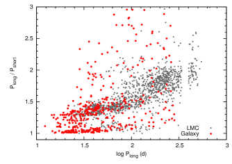
Figure 15: Petersen diagram plotting $\log P_{\rm long}$ against the ratio of $P_{\rm long}$ to $P_{\rm short}$ for adjacent periods (red) in galactic M giants (S/N $\geq 10$). Data for the LMC (Derekas et al., 2006) are plotted in grey.

Period ratios provide a useful mechanism to compare the pulsational behaviour of local SRVs to those in the lower metallicity environment of the LMC, since they are independent of distance. Figure 15 plots a Petersen diagram for all multi-periodic stars in our sample (S/N $\geq 10$). Each red point represents the ratio of a longer period to the shorter, plotted against the log of the longer period. For comparison, we have plotted the period ratios of LMC MACHO red giants (Derekas et al., 2006, grey points), which show a striking similarity. The most densely populated region occurs at a period ratio of about 1.3, corresponding to first and second radial overtone modes ($P_{1}/P_{2}$) in the theoretical model of Wood & Sebo (1996). The ratio is in excellent agreement with the MACHO data, and is one of the most common period ratios found by Soszyński et al. (2004) in their analysis of period ratios in OGLE observations of the LMC.

The other significant overlap occurs for period ratios close to 1. Although the MACHO data contain few short-period ($\log P<1.4$) stars in this region, the analysis of OGLE data by Soszyński et al. (2004) appears to have identified many more variables, and their Petersen diagram (fig 11) shows a large number of stars extending to $\log P\sim 1.1$, in agreement with our local SRVs. A small period ratio has many possible interpretations, including two closely separated oscillation modes, high-overtone radial pulsation, a single, slightly varying period, or may be an artefact of amplitude or phase modulation. The former interpretation may imply the presence of non-radial oscillation modes (Kiss & Lah, 2006). However, as noted earlier, our data include multiple closely spaced periods that probably represent the same oscillation mode, which will result in the small period-ratios being over represented in our Petersen diagram, although this is somewhat reduced by the use of periods with S/N $\geq$ 10.

The area of minimal overlap with LMC data around $\log P\sim$ 2.4 and period ratios of $\sim$ 1.9 is most likely due to our sample selection, which excluded stars with GCVS periods longer than 100 d. Although they have no obvious analogue in the MACHO data, we note that the small group of stars with period ratios of $\sim$ 1.9 (and $\log\;P\sim 1.6$) do appear in the larger LMC sample of Soszyński et al. (2004). Furthermore, our period ratios are consistent with those found by Wray, Eyer & Paczyński (2004), who demonstrated that ratios of $\sim$ 1.0, 1.1, 1.3, and 1.9 are common amongst pulsating red giants in the galactic bulge.

8 Conclusion & future work

A fully autonomous instrument has been designed, built, and operated for 5.5 years for a unique, homogenous survey of the nearest M giant stars. The main results of this paper are the following:

1. We have determined the characteristic pulsation periods of 247 bright, nearby, M giants, the majority of which have not been determined previously, thereby increasing the number of such stars by a factor of 4.

2. We provide updated $K$-band magnitudes, selected from several NIR sources, which we carefully compared to determine the most reliable values. We include the effect of interstellar extinction and show that circumstellar extinction can be ignored.

3. We employ a novel technique to correct residual errors in our flat-fielding images, and successfully use Optimal Image Subtraction for a subset of blended stars, yielding scintillation-limited differential photometry to better than 1% precision.

4. Twenty-three stars were observed concurrently with PEP and are in excellent agreement with the CCD data. Moreover, 21 stars in our sample had periods determined previously, and a comparison with literature values showed our periods to be in good agreement.

5. All stars in the sample were found to be variable, leading us to conclude that the Hipparcos variability flag, which was used to select the sample, is a good predictor of variability.

6. Many stars in the sample exhibit closely spaced periods (period ratios $<$ 1.1), similar to those seen in solar-like stars, which probably represent changes in amplitude and/or phase of a single oscillation mode.

7. Eighty-seven percent of the stars were found to be multi-periodic, with the modal number of periods being 2 (S/N $\geq$ 10) and 3 (S/N $\geq$ 7.5).

8. The period ratios of local M giants were compared to multi-periodic stars in the LMC and Bulge, and were found to be in excellent agreement.

Our motivation for conducting this survey was to significantly increase the sample of nearby M giants to enable unambiguous identification of the local P-L sequences, and to determine the metallicity dependence of the P-L zero-point. These issues will be discussed in Paper II.

Acknowledgments

We extend our thanks to Aliz Derekas for kindly supplying her LMC data for Figure 15. This research has made use of the VizieR and SIMBAD databases, operated at CDS, Strasbourg, France. This project has been supported by the Australian Research Council and the Hungarian OTKA Grant K76816.

Appendix A Light curves

Figure 17: Power spectra corresponding to the light curves in Figure 16. Insets show the spectral window using the same horizontal scale as the main plot. A horizontal line shows the mean signal in the frequency range 0.20–0.40 cycle d^-1. Peaks corresponding to periods listed in Table LABEL:T4 are indicated with dotted lines.

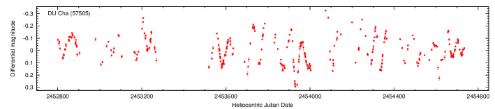
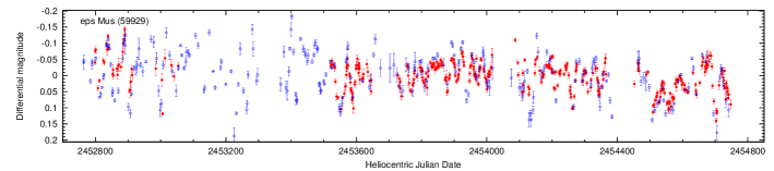
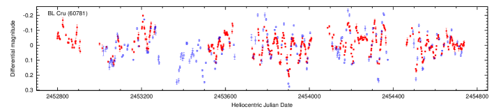
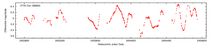
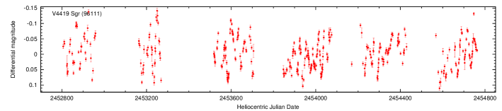
Figure 18: A selection of light curves.

Figure 19: Power spectra corresponding to the light curves in Figure 18.

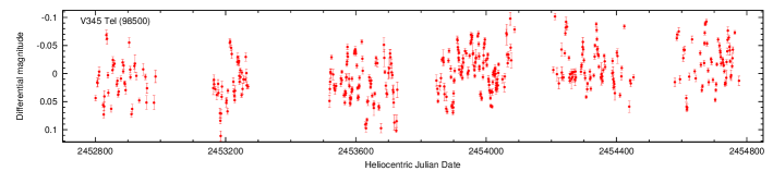
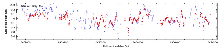
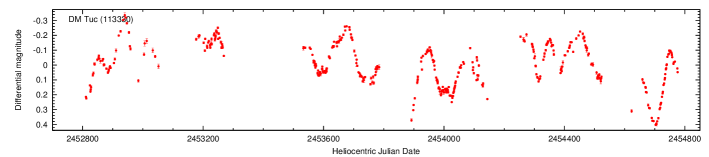
Figure 20: A selection of light curves and corresponding power spectra.

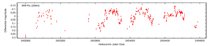
Figure 21: Power spectra of selected stars exhibiting short-period pulsation (top 3 panels). The bottom panel is a light curve of WW Pic which exhibits a long secondary period of $\sim$ 370 d and a shorter 36-d period.

References

- Alard & Lupton (1998) Alard, C., Lupton, R.H., 1998, ApJ, 503, 325
- Balona (1995) Balona, L.A., 1995, IAU Symp., 167, 187
- Bedding & Zijlstra (1998) Bedding, T.R., Zijlstra, A.A., 1998, ApJ, 506, L47
- Bedding et al. (2005) Bedding, T.R., Kiss, L.L., Kjeldsen, H., Brewer, B.J., Dind, Z.E., Kawaler, S.D., Zijlstra, A.A., 2005, MNRAS, 361, 1375
- Berry & Burnell (2000) Berry, R., Burnell, J., 2000, Astronomical Image Processing, Willmann-Bell, Richmond, VA, U.S.A.
- Bessell & Brett (1988) Bessell, M.S., Brett, J.M., 1988, PASP, 100, 1131
- Boyle et al. (2003) Boyle, R.P., Janusz, R., Davis Philip, A.G., Kazlauskas, A., Laugalys, V., 2003, Baltic Astronomy, 12, 476
- Chromey & Hasselbacher (1996) Chromey, F.R., Hasselbacher, D.A., 1996, PASP, 108, 944
- Cutri et al. (2003) Cutri, R.M. et al., 2003, Explanatory Supplement to the 2MASS All Sky Data Release, Caltech, Pasadena
- Derekas et al. (2006) Derekas, A., Kiss, L.L., Bedding, T.R., Kjeldsen, H., Lah, P., Szabó, Gy. M., 2006, ApJ, 650, L55
- Drimmel, Cabrera-Lavers & López-Corredoira (2003) Drimmel, R., Cabrera-Lavers, A., López-Corredoira, M., 2003, A&A, 409, 205
- Eggen (1975) Eggen, O.J., 1975, ApJ, 195, 661
- Everett & Howell (1975) Everett, M.E., Howell, S.B., 2001, PASP, 113, 1428
- Eyer & Mowlavi (2008) Eyer, L., Mowlavi, N., 2008, JPhCS, 118, 1201
- Frandsen et al. (1995) Frandsen, S., Jones, A., Kjeldsen, H., Viskum, M., Hjorth, J., Andersen, N.H., Thomsen, B, 1995, A&A, 301, 123
- Gilliland et al. (1993) Gilliland, R.L. et al., 1993, AJ, 106, 2441
- Gezari et al. (1999) Gezari, D.Y., Pitts, P.S., Schmitz, M., 1999, Catalog of Infrared Observations, Edition 5
- Glass & Lloyd-Evans (1981) Glass, I.S., Lloyd-Evans, T.L., 1981, Nature, 291, 303
- Glass & van Leeuwen (2007) Glass, I.S., van Leeuwen, F., 2007, MNRAS, 378, 1543
- Groenewegen (2004) Groenewegen, M.A.T., 2004, A&A, 425, 595
- Hakkila et al. (1997) Hakkila, J., Myers, J.M., Stidham, B.J., Hartmann, D.H., 1997, AJ, 114, 2043
- Hoffleit & Warren (1991) Hoffleit, D., Warren, Jr W.H., 1991, The Bright Star Catalogue, 5th Revised Ed., Online-only reference: http://cdsarc.u-strasbg.fr/viz-bin/Cat?V/50
- Houk (1982) Houk, N., 1982, Catalogue of two-dimensional spectral types for the HD Stars, Volume 3, Online-reference: http://cdsarc.u-strasbg.fr/viz-bin/Cat?III/80
- Houk & Smith-Moore (1988) Houk, N., Smith-Moore, M., 1988, Michigan Catalogue of Two-dimensional Spectral Types for the HD Stars, Volume 4, Online-reference: http://cdsarc.u-strasbg.fr/viz-bin/Cat?III/133
- Israel et al. (2007) Israel, H., Hessman, F.V., Schuh, S., 2007, AN, 328, 16
- Ita et al. (2004) Ita Y., et al., 2004, MNRAS, 347, 720
- Kiss et al. (1999) Kiss, L.L., Szatmáry, K., Cadmus, R.R. Jr, Mattei, J.A., 1999, A&A, 346, 542
- Kiss et al. (2000) Kiss, L.L., Szatmáry, K., Szabó, G., Mattei, J.A., 2000, A&AS, 145, 283
- Kiss & Bedding (2003) Kiss, L.L., Bedding, T.R., 2003, MNRAS, 343, L79
- Kiss & Bedding (2004) Kiss, L.L., Bedding, T.R., 2004, MNRAS, 347, L83
- Kiss & Lah (2006) Kiss, L.L., Lah, P., 2006, Mem. S.A.It., 77, 303
- Knapp et al. (2003) Knapp, G.R., Pourbaix, D., Platais, I., Jorissen, A., 2003, A&A, 403, 993
- Kochanski et al. (1996) Kochanski, G.P., Tyson, A., Fischer, P., 1996, AJ, 111, 1444
- Manfroid (1995) Manfroid, J., 1995, A&AS, 113, 587
- Mattei et al. (1997) Mattei, J.A. et al., 1997, ESA-SP, 402, 269
- Mermilliod et al. (1997) Mermilliod, J.C., Hauck, B., Mermilliod M. 1997, A&AS, 124, 349, General Catalogue of Photometric Data II
- Moon, Otero & Kiss (2007) Moon, T.M., Otero, S.A., Kiss, L.L., 2007, JAAVSO, 36, 71
- Oliver & Wood (2003) Olivier, E.A., Wood, P.R., 2003, ApJ, 584, 1035
- Percy et al. (2003) Percy, J.R., Besla, G., Velocci, V., Henry, G.W., 2003, PASP, 115, 479
- Perryman et al. (1997) Perryman, M.A.C. et al., 1997, A&A, 323, L49
- Pickles (1998) Pickles, A.J., 1998, PASP, 110, 863
- Pojmański (1997) Pojmański, G., 1997, AcA, 47, 467
- Rest et al. (2002) Rest A., Mündermann, L., Widenhorn, R., Bodegom, E., McGlinn, T.C., 2002, Rev. Sci. Instrum, 73, 2028
- Rieke & Lebofsky (1985) Rieke, G.H., Lebofsky, M.J., 1985, ApJ, 288, 618
- Robertson & Feast (1981) Robsertson, B.S.C., Feast, M.W., 1981, MNRAS, 196, 111
- Samus et al. (2009) Samus, N.N. et al., General Catalog of Variable Stars (GCVS database, Version 2009-Mar), Online-only reference: http://cdsarc.u-strasbg.fr/viz-bin/Cat?B/gcvs
- Scargle (1989) Scargle, J.D, 1989, ApJ, 343, 874
- Schlegel et al. (1998) Schlegel, D.J., Finkbeiner, D.P., Davis, M., 1998, ApJ, 500, 525
- Skiff (2009) Skiff, B.A., 2009, General Catalogue of Stellar Spectral Classifications (Version 2009-Feb), Online-only reference: http://cdsarc.u-strasbg.fr/viz-bin/Cat?B/mk
- Smith et al. (2004) Smith, B.J., Price, S. D., Baker, R.I., 2004, ApJS, 154, 673
- Soszyński et al. (2004) Soszyński, I., Udalski, A., Kubiak, M., Szymański, M., Pietrzyński, G., Żebruń, K., Szewczyk, O., Wyrzykowski, Ł., 2004, AcA, 54, 129
- Soszyński et al. (2007) Soszyński, I. et al., 2007, AcA, 57, 201
- Szeidl et al. (1992) Szeidl, B., Oláh, K., Szabados, L., Barlai, K., Patkós, L., 1992, Comm. Konkoly Obs., 97, 245
- Tabur et al. (2002) Tabur, V., Liller, W., Jones, A., Marang, F., 2002, IAUC 8001
- Tabur & Monard (2003a) Tabur, V., Monard, L.A.G., 2003, IAUC 8184
- Tabur et al. (2003b) Tabur, V., Lovejoy, T., Broughton, J., Higgins, D., 2003, IAUC 8223
- Tabur (2007) Tabur, V., 2007, PASA, 24, 189
- van Leeuwen & Fantino (2005) van Leeuwen, F., Fantino, E., 2005, A&A, 439, 791
- van Leeuwen (2007) van Leeuwen, F., 2007, Ap&SS Library, Vol. 350, Hipparcos, the New Reduction of the Raw Data, Springer, Berlin
- Wallace & Tritton (1979) Wallace, P.T., Tritton, K.P., 1979, MNRAS, 189, 115
- Woźniak et al. (2004) Woźniak, P.R. et al, 2004, AJ, 127, 2436
- Whitelock et al. (2008) Whitelock, P.A., Feast, M.W., van Leeuwen, F., 2008, MNRAS, 386, 313
- Wood & Sebo (1996) Wood, P.R., Sebo, K.M., 1996, MNRAS, 282, 958
- Wood et al. (1999) Wood, P.R. et al., 1999, IAU Symp., 191, 151
- Wood et al. (2004) Wood, P.R., Olivier, E.A., Kawaler, S.D., 2004, ApJ, 604, 800
- Wray, Eyer & Paczyński (2004) Wray, J.J., Eyer, L., Paczyński, B., 2004, MNRAS, 349, 1059
- Yeşilyaprak & Aslan (2004) Yeşilyaprak, C., Aslan, Z., 2004, MNRAS, 355, 601
- Young (1967) Young, A.T., 1967, AJ, 72, 747
- Zhou et al. (2004) Zhou, X. et al., 2004, AJ, 127, 3642
- Zissell (2000) Zissell, R.E., 2000, JAAVSO, 28, 149