Perturbation Analysis of a General Polytropic
Homologously Collapsing Stellar Core

Abstract

For dyanmic background models of Goldreich & Weber and Lou & Cao, we examine three-dimensional perturbation properties of oscillations and instabilities in a general polytropic homologously collapsing stellar core of a relativistically hot medium with a polytropic index $\gamma=4/3$. Perturbation behaviours, especially internal gravity g$-$modes, depend on the variation of specific entropy in the collapsing core. Among possible perturbations, we identify acoustic p$-$modes and surface f$-$modes as well as internal gravity g${}^{+}-$modes and g${}^{-}-$modes. As in stellar oscillations of a static star, we define g${}^{+}-$ and g${}^{-}-$modes by the sign of the Brunt-V$\ddot{\rm a}$is$\ddot{\rm a}$l$\ddot{\rm a}$ buoyancy frequency squared ${\cal N}^{2}$ for a collapsing stellar core. A new criterion for the onset of convective instabilities is established for a homologous stellar core collapse. We demonstrate that the global energy criterion of Chandrasekhar is insufficient to warrant the stability of general polytropic equilibria. We confirm the acoustic p$-$mode stability of Goldreich & Weber, even though their p$-$mode eigenvalues appear in systematic errors. Unstable modes include g${}^{-}-$modes and sufficiently high-order g${}^{+}-$modes, both corresponding to convective core instabilities. Such instabilities occur before the stellar core bounce, in contrast to instabilities in other models of supernova (SN) explosions. The breakdown of spherical symmetry happens earlier than expected in numerical simulations so far. The formation and motion of the central compact object are speculated to be much affected by such g$-$mode instabilities. By estimates of typical parameters, unstable low-order $l=1$ g$-$modes may produce initial kicks of the central compact object. Other high-order and high-degree unstable g$-$modes may shred the nascent neutron core into pieces without an eventual compact remnant (e.g. SN1987A). Formation of binary pulsars and planets around neutron stars might originate from unstable $l=2$ g$-$modes and high-order high-degree g$-$modes, respectively.

1 Introduction

Supernovae (SNe), hypernovae and a few detected SNe associated with long gamma-ray bursts (GRBs) serve as important cornerstones of several major branches in astrophysics and cosmology. Physical mechanisms and outcomes for such violent explosions of massive stars have been actively pursued for decades. Hydrodynamics and magnetohydrodynamics (MHD) together with simplifying approximations and increasingly sophisticated microphysics have been invoked to model various aspects of SNe in both analytic treatments and numerical simulations. As nuclear fuels eventually become insufficient in the stellar core, the process of core-collapse SNe signaling the demise of massive progenitors (e.g. red and blue giants) may be conceptually divided into three stages of core collapse, rebound shock and neutrino heating (e.g. Burrows et al. 1995; Janka & Müller 1996).

The fortuitous detection of neutrinos from SN1987A (Hirata et al. 1987; Bionta et al. 1987; Koshiba 2009 private communications), bolsters such a scenario framework in part or as a whole. Optical observations before SN1987A revealed its progenitor as a blue giant star in a mass range of $\sim 16-22M_{\odot}$ (e.g. Arnett et al. 1989). At the time of SN1987A explosion, twenty neutrinos in the energy range of $\sim 6-39$ MeV were intercepted within $\sim 12$ s, confirming the occurrence of neutronization. The timescale of neutrino emissions was consistent with the prediction for neutrino trapping inside an extremely dense collapsed core. The total neutrino flux was consistent with energetic neutrinos carrying off the binding energy during the core neutronization (Chevalier 2009 private communications), even though no signals of a neutron star (e.g. a pulsar) or a black hole are detected (McCray 2009 private communications).

In spite of extensive research on analytic and numerical studies of SNe over several decades (e.g. Goldreich & Weber 1980 – GW hearafter; Yahil 1983; Bruenn 1985; Bruenn 1989a, b; Herant et al. 1995; Janka & M${\rm\ddot{u}}$ller 1995, 1996; Fryer & Warren 2002, 2004; Blondin, Mezzacappa & DeMarino 2003; Blondin & Mezzacappa 2006; Burrows et al. 2006, 2007a, b; Lou & Wang 2006, 2007; Wang & Lou 2007, 2008; Lou & Cao 2008; Hu & Lou 2009), a few major issues in the SN model development remain to be explored (see Burrows et al. 2007 for a recent review). Among these theoretical challenges, the dynamics of core-collapse stage inside the progenitor and the possibility of convective instabilities during this phase are the main thrust of this paper.

The simplest hydrodynamic model to describe a core collapse is a one-dimensional radial contraction with spherical symmetry under the self-gravity. In analytical model analyses, approximations to the equation of state (EoS) for gas medium are necessarily introduced. It can be shown in statistical mechanics (e.g. Huang 1987) that a relativistic hot Fermi gas with a temperature much lower than the Fermi energy can be modelled by a simple $\gamma=4/3$ polytropic EoS with $\gamma$ being the polytropic index (i.e. the rest mass of a single particle $\ll$ the kinetic energy of a particle $\ll$ the Fermi energy). This approximate EoS also gains support in numerical simulations (e.g. Bethe et al. 1979; Hillebrandt, Nomoto & Wolff 1984; Shen et al. 1998). For instance, Bethe et al. (1979) concluded that as the neutrino trapping occurs, relativistic electrons, high-energy photons and neutrinos mainly contribute to the total pressure within a collapsing stellar core under gravity. As nuclei start to ``feel" each other at a high density reaching up to $\sim 2.7\times 10^{14}{\rm g\ cm^{-3}}$, the stiffness of nuclear matter adjusts the polytropic index $\gamma$ to $\sim 2.5$.

There are two kinds of polytropic approximations. One is the conventional polytropic EoS with $P=\kappa\rho^{\gamma}$ ($P$ and $\rho$ are pressure and mass density, respectively) where $\kappa$ remains constant in space and time. The other is a general polytropic EoS where $\kappa$ remains constant along streamlines, i.e.

$$\left(\frac{\partial}{\partial t}+\bf{u}\cdot\nabla\right)\left(\frac{P}{\rho^{\gamma}}\right)=0\ ,$$

where ${\bf u}$ is the bulk flow velocity. The former is actually a special case of the latter, although we treat them separately. It is easy to prove that for a relativistic hot Fermi gas with a temperature much lower than the Fermi energy, the specific entropy of the material is a function of $\log(P/\rho^{\gamma})$ (see footnote 1). In other words, the former EoS is interpreted as a constant specific entropy while the latter bears a variable distribution of specific entropy. The latter general polytropic EoS obeys the conservation of specific entropy along streamlines. The gas dynamics involves the competition between self-gravity and pressure gradient force. Such models give rise to various self-similar solutions by which the flow system partially loses its memory of initial and boundary conditions (e.g. Larson 1969; Penston 1969; Shu 1977; Cheng 1978; GW; Yahil 1983; Suto & Silk 1988; Lou & Shen 2004; Yu et al. 2006; Lou & Wang 2006, 2007; Wang & Lou 2007, 2008; Lou & Cao 2008; Hu & Lou 2009). For core-collapse SNe, GW studied the homologous stellar core collapse of a $\gamma=4/3$ conventional polytropic gas. They concluded that starting from a static core, if the pressure is reduced by no more than $\sim 2.9\%$, the central core will evolve into a homologously collapsing phase. This fraction is much less than $\sim 26\%$ as indicated by Bethe et al. (1979). Yahil (1983) extended GW analysis to $\gamma\leq 4/3$ conventional polytropic cases and noted the existence of an outer envelope moving inwards with a supersonic speed. One important difference between GW and Yahil (1983) is that solutions of the former have outer boundaries with zero mass density there while those of the latter extend to infinity (Lou & Cao 2008).

With a similarity transformation (Fatuzzo et al. 2004), Lou & Cao (2008) extended homologous core collapse to general polytropic cases. This is a substantial theoretical development of the model framework because several studies (e.g. Bethe et al. 1979; Bruenn 1985, 1989b; Burrows et al. 2006; Hillebrandt et al. 1984; Janka & M$\ddot{\rm u}$ller 1995, 1996; Shen et al. 1998) on EoS with microphysics during SNe do suggest variable specific entropy depending on physical conditions, including density, temperature and metallicity.

Meanwhile, extensive numerical simulations show that spherically symmetric models cannot initiate SN explosions with an energy of $\sim 10^{52}{\ \rm ergs}$ (e.g. Janka & M$\ddot{\rm u}$ller 1995, 1996; Kitaura, Janka & Hillebrandt 2006) partly because the SN explosion energy appears insufficient and partly because instabilities occur in multi-dimensional simulations. The role of instabilities and symmetry breaking in SNe has now been emphasized (e.g. Burrows 2000, 2006). Along this line, various instabilities were proposed (e.g. Goldreich, Lai & Sahrling 1996; Lai 2000; Lai & Goldreich 2000; Murphy, Burrows & Heger 2004; Blondin et al. 2003; Blondin & Mezzacappa 2006) and several mechanisms may provide seed fluctuations before and during SN explosions (e.g. Bazan & Arnett 1998; Meakin & Arnett 2006, 2007a, b). Prior to the onset of a core collapse, the so-called ``$\epsilon$-mechanism" (e.g. Goldreich et al. 1996; Murphy et al. 2004) may lead to g$-$mode overstabilities in the progenitor, due to the overreaction of nuclear processes against perturbations.

Lai & Goldreich (2000) found an instability in the outer supersonic envelope during the collapsing phase. They performed both analytical and numerical irrotational perturbation analysis using the conventional polytropic EoS for collapsing solutions including EWCS of Shu (1977) and post-collapse solution of Yahil (1983), and found instabilities in supersonic regions. In their derivation, the perturbed flow was assumed irrotational (i.e. without vorticity) and thus g$-$modes should have been excluded. In an example, they initiated their calculation with a g$-$mode perturbation; this initial condition appears to contradict the constraints of their analytical derivations and numerical analysis. After the emergence of a rebound shock, several instabilities have been suggested. Intense convective motions may be sustained outside the neutrino sphere (e.g. Herant, Benz & Colgate 1992; Herant et al. 1994). Standing accretion shock instability (hereafter SASI; e.g. Foglizzo 2001) appears around $\sim 200$ ms after the core bounce in some simulations (e.g. Blondin & Mezzacappa 2006; Blondin et al. 2003). Burrows et al. (2006, 2007a, b) proposed that $l=1$ g$-$modes at $\sim 500$ ms after the stellar core bounce may serve as an agent to extract the gravitational energy for the kinetic energy of SNe. The roles of these instabilities are still hotly debated and a successful SN explosion requires further explorations.

No significant core instabilities were reported for the core-collapse phase. Linear stability analyses were performed by GW, Lai (2000) and Lai & Goldreich (2000) for certain dynamic flows. GW perturbed their homologously collapsing solutions and concluded that this collapse is stable for acoustic p$-$modes with the g$-$modes being neutral convective modes. Lai (2000) extended this acoustic stability analysis to solutions of Yahil (1983) and found no unstable modes for $\gamma\simeq 4/3$ cases in numerical explorations. Lai & Goldreich (2000) studied the stability of collapsing core and claimed that the core remains stable in subsonic regions while the envelope becomes unstable in supersonic regions. All these stable core statements relies on the assumption of a conventional polytropic EoS. Conventional polytropic gas flows and perturbations correspond to a constant specific entropy and make g$-$modes just neutral convective modes.

Our main theme is to examine stability properties of a stellar core collapse with a variable specific entropy distribution in a homologously collapsing model (Lou & Cao 2008). By numerical explorations, we classify various perturbation modes including p$-$modes and g$-$modes (e.g. Cowling 1941), some of which are oscillatory while others grow with time in power laws. As the hydrostatic equilibrium is a limiting case of our model, we find connection and evolution between perturbations in progenitors of hydrostatic case and dynamic collapsing stage. The most interesting result is that some stable g$-$modes in the static case become unstable in the dynamically collapsing stage. In particular, the stability of each mode now becomes sensitive to the self-similar evolution of specific entropy. This instability occurs during the core-collapse phase, neither before the core collapse nor after the core bounce. We speculate implications of such core instabilities during the collapse phase. For example, the $l=1$ unstable g$-$mode may lead to the kick velocity of a pulsar.

SN explosions involve a chain of physical processes. The spherical symmetry may be destroyed by a series of instabilities in the progenitor during the entire SN explosion. For example, overstable g$-$modes of Goldreich et al. (1996) and Murphy et al. (2004) may provide seed g$-$mode perturbations during the core collapse. Perturbations of our model may connect to further instabilities after the core bounce and the emergence of an outgoing shock. Our model results are highly suggestive and can be tested numerically.

This paper is structured as follows. Section 2 describes general polytropic solutions of spherically symmetric homologous core collapse, as a generalization of GW results. Homogeneous ordinary differential equations (ODEs) for three-dimensional (3D) general polytropic perturbations are obtained in Section 3. Numerical results are analyzed in Section 4. We consider several aspects of SNe in Section 5 and conclude in Section 6. Mathematical details are summarized in Appendices A$-$C for the convenience of reference.

2 Spherical Homologous Stellar Core Collapses

Before starting the time-dependent 3D general polytropic perturbation analysis, we first briefly summarize homologous core collapse solutions with spherical symmetry of Lou & Cao (2008), making some notational adjustments in our model development for the convenience of comparison with GW results. The nonlinear partial differential equations (PDEs) for ideal hydrodynamics are conservations of momentum and mass, Poisson equation for the gravitational field and a general polytropic EoS, viz.

$$\frac{\partial{\bf u}}{\partial t}+({\bf u}\cdot\nabla){\bf u}=-\frac{1}{\rho}\nabla P-\nabla\Phi\ ,$$ (1)

$$\frac{\partial\rho}{\partial t}+\nabla\cdot\left(\rho{\bf u}\right)=0\ ,$$ (2)

$$\nabla^{2}\Phi=4\pi G\rho\ ,$$ (3)

$$P=\kappa({\bf r},\ t)\rho^{\gamma}\ ,\qquad\quad\left(\frac{\partial}{\partial t}+{\bf u}\cdot\nabla\right)\log\kappa=0\ ,$$ (4)

where ${\bf u}({\bf r},\ t)$, $P({\bf r},\ t)$, $\rho({\bf r},\ t)$ and $\Phi({\bf r},\ t)$ are bulk flow velocity, gas pressure, mass density and gravitational potential of the flow system, respectively and $G=6.67\times 10^{-8}$ cm${}^{3}/$(g s²) is the universal gravitational constant, and $\gamma=4/3$ is the polytropic index for a relativistically hot gas.

It is known that these ideal nonlinear hydrodynamic PDEs are invariant under the time reversal operation,

$$t\rightarrow-t,\quad{\bf u}\rightarrow-{\bf u},\quad\rho\rightarrow\rho,\quad P\rightarrow P,\quad\Phi\rightarrow\Phi\ .$$ (5)

This property enables us to use an outflow solution to also describe a collapse process, which is very important to understand homologous core collapse in terms of these expressions for the time reversal invariance.

To generalize the analysis of GW model of spherical symmetry, we introduce the following time-dependent spatial scale factor $a(t)$,

$$a(t)=\rho_{c}(t)^{-1/3}\left(\frac{\kappa_{c}}{\pi G}\right)^{1/2}\ ,$$ (6)

where time-dependent $\rho_{c}(t)$ and constant coefficient $\kappa_{c}$ are the values of $\rho$ and $\kappa$ at the core centre of a massive progenitor star (thus the subscript _c). The dimensional vector radius $\vec{r}$ is scaled to a dimensionless vector radius ${\bf x}=\vec{r}/a(t)$. Consistently, flow variables of ${\bf u}(r,\ t)$, $P(r,\ t)$, $\rho(r,\ t)$ and $\Phi(r,\ t)$ are assumed to take on the following forms of

$${\bf u}=\dot{a}(t){\bf x}\ ,$$ (7)

$$\rho=\rho_{c}(t)f^{3}(x)=\left(\frac{\kappa_{c}}{\pi G}\right)^{3/2}a^{-3}f^{3}(x)\ ,$$ (8)

$$P=\kappa\rho^{4/3}=\frac{\kappa_{c}^{3}}{(\pi G)^{2}}a^{-4}g(x)f^{4}(x)\ ,$$ (9)

$$\Phi=\frac{4}{3}\left(\frac{\kappa_{c}^{3}}{\pi G}\right)^{1/2}a^{-1}\psi(x)\ ,$$ (10)

where $\kappa(r,\ t)$ is prescribed in the form of $\kappa_{c}g(x)$ with a constant $\kappa_{c}$. The central mass density $\rho_{c}(t)$ is proportional to $a^{-3}(t)$ and varies with $t$. Substituting expressions (7)$-$(10) into nonlinear PDEs $(\ref{g1})-(\ref{g4})$ under spherical symmetry with $x=r/a(t)$, we reduce these nonlinear PDEs to a set of coupled nonlinear ODEs. First, PDEs (1) and (4) are automatically satisfied, the latter of which means that $g(x)$ can be of an arbitrary form. For example, $g(x)=1$ brings our general polytropic EoS back to the conventional polytropic EoS with a constant coefficient $\kappa=\kappa_{c}$ studied by GW. Momentum equation (1) then leads to

$$-\left(\frac{\pi G}{\kappa_{c}^{3}}\right)^{1/2}a^{2}\ddot{a}=\frac{1}{x}\left[\frac{1}{f^{3}}\frac{d}{dx}\left(gf^{4}\right)+\frac{4}{3}\frac{d\psi}{dx}\right]\ ,$$ (11)

where the left-hand side (LHS) depends only on $t$ while the right-hand side (RHS) depends only on $x$. For consistency, we therefore need to set both sides equal to a constant $4\lambda/3$ and obtain two separate nonlinear ODEs, viz.

$$-\left(\frac{\pi G}{\kappa_{c}^{3}}\right)^{1/2}a^{2}\ddot{a}=\frac{4}{3}\lambda\ ,$$ (12)

$$\frac{d\psi}{dx}=\lambda x-\frac{3}{4f^{3}}\frac{d}{dx}\left(gf^{4}\right)\ .$$ (13)

ODE (12) indicates that the spatial scale factor $a(t)$ is either a constant independent of $t$ with $\lambda=0$ or a power law of $t$ being proportional to $t^{2/3}$. Substituting equation (13) into Poisson equation (3), we derive an ODE for $f(x)$, viz.

$$\frac{1}{x^{2}}\frac{d}{dx}\left[\frac{x^{2}}{f^{3}}\frac{d}{dx}\left(gf^{4}\right)\right]+4f^{3}=4\lambda\ ,$$ (14)

which gives a profile of mass density $\rho$ by eq (8) at time $t$ and radius $r$ because $x$ is the independent similarity variable combining $t$ and $r$ together. Once $f(x)$ is known, other variables can all be readily derived. The special case of $\lambda=0$ leads to the limit of general polytropic Lane-Emden equation (e.g. Eddington 1926; Chandrasekhar 1939) and $\lambda>0$ describes outflows or collapses by the time reversal operation. For a necessary check, $g(x)=1$ in ODE (14) reduces to equation (16) of GW precisely as expected.

The `boundary conditions' for second-order nonlinear ODE (14) are as follows. The radial gradient of pressure should vanish at the centre, i.e.

$$\nabla P|_{x=0}=0\qquad\ \Rightarrow\qquad\ 4f^{\prime}(0)+g^{\prime}(0)=0\ ,$$ (15)

where the prime ^′ indicates the first derivative in terms of the self-similar independent variable $x$. In order to obtain a physically sensible solution of $f(x)$ related to the mass density by algebraic expression (8), we require an outer boundary $x_{b}$ which is the smallest value of solutions $f(x)=0$. The reason is, if no solution is found for $f(x)=0$ at a finite $x>0$, it means that the system extends to infinity. Therefore, the dimensional velocity ${\bf u}=2\vec{r}/(3t)$ will diverge towards extremely large radii. Such a divergent flow velocity is unacceptable in realistic astrophysical gas systems.

Hence, these boundary conditions determine a continuous range of $\lambda$ values and the maximum acceptable value of $\lambda$, denoted by $\lambda_{M}$ hereafter, corresponding to a solution $f(x)$ where $f^{\prime}(x_{b})=0$ also at the outer boundary $f(x_{b})=0$. By numerical explorations, solution $f(x)$ for $\lambda>\lambda_{M}$ does not go to zero at a finite $x$ but oscillate with decreasing amplitude with increasing $x$. Different profiles of $g(x)$ will lead to different values of $\lambda_{M}$. For the special case of $g(x)=1$, the $\lambda$ range is $0\leq\lambda\leq\lambda_{M}=0.00654376$ which was first determined by GW and also confirmed by Lou & Cao (2008) with a corresponding $f_{c}\equiv f(0)=4.67047$.

The local polytropic sound speed is defined by

$$V_{s}=\bigg{(}\frac{\partial P}{\partial\rho}\bigg{)}^{1/2}\propto\big{[}g(x)\rho^{1/3}\big{]}^{1/2}\ .$$ (16)

In the theory of stellar oscillations, it is required that the sound speed at the centre approaches a finite value (e.g. Unno et al. 1979). We impose the same condition for a dynamic collapse. Hence, $g^{\prime}(0)=0$ and therefore $f^{\prime}(0)=0$.

Once $f(x)$ is obtained, it is straightforward to calculate the total enclosed mass of the collapsing core and the ratio between the mean mass density and the central mass density in terms of $f^{\prime}(x_{b})$ and $x_{b}$. The total enclosed mass $M$ of the collapsing core is given by

$$M\!\!\!\!\! = \!\!\!\!\!\int_{0}^{r_{b}}4\pi r^{2}\rho dr=\frac{4}{3}\pi x_{b}^{3}\left(\frac{\kappa_{c}}{\pi G}\right)^{3/2}\left[\lambda-\frac{3}{x_{b}}g(x_{b})f^{\prime}(x_{b})\right]$$ (17)

$$= \!\!\!\!\!\frac{4}{3}\pi x_{b}^{3}\left(\frac{\kappa_{c}}{\pi G}\right)^{3/2}\frac{\bar{\rho}}{\rho_{c}}\ ,$$

where the ratio between the mean mass density $\bar{\rho}$ and the central mass density $\rho_{c}$ is readily identified with

$$\frac{\bar{\rho}}{\rho_{c}}=\lambda-\frac{3}{x_{b}}g(x_{b})f^{\prime}(x_{b})\ .$$ (18)

The mean mass density $\bar{\rho}$ varies with $t$ because $r_{b}$ decreases with $t$ for a homologous stellar core collapse. For $\lambda=\lambda_{M}$, we have $f^{\prime}(x_{b})=0$ and therefore ${\bar{\rho}}/{\rho_{c}}=\lambda_{M}$.

3 Three-Dimensional Perturbations

We now consider 3D general polytropic perturbations to the background self-similar hydrodynamic collapse described in the previous section in spherical polar coordinates $(r,\ \theta,\ \varphi)$. Flow variables including small perturbations are assumed to bear the following forms of

$${\bf u}=\dot{a}(t){\bf x}+\frac{a}{t_{ff}}{\bf v}_{1}(x,\ \theta,\ \varphi)\tau(t)\ ,$$ (19)

$$\rho=\left(\frac{\kappa_{c}}{\pi G}\right)^{3/2}a(t)^{-3}f^{3}(x)[1+f_{1}(x,\ \theta,\ \varphi)\tau(t)]\ ,$$ (20)

$$P=\frac{\kappa_{c}^{3}}{(\pi G)^{2}}a(t)^{-4}g(x)f^{4}(x)[1+\beta_{1}(x,\ \theta,\ \varphi)\tau(t)]\ ,$$ (21)

$$\Phi=\frac{4}{3}\left(\frac{\kappa_{c}^{3}}{\pi G}\right)^{1/2}a(t)^{-1}[\psi(x)+\psi_{1}(x,\ \theta,\ \varphi)\tau(t)]\ ,$$ (22)

where the subscript $1$ indicates associations with perturbation terms which are small compared to the background dynamic flow variables and the free-fall timescale $t_{ff}$ is itself time-dependent and is written in the specific form of

$$t_{ff} = \left(\frac{4}{3}\pi G\rho_{c}\right)^{-1/2}\qquad\qquad{\rm for\ all\ \lambda}$$ (23)

$$= \left(\frac{9\lambda}{2}\right)^{1/2}t\qquad\qquad\qquad{\rm for\ \lambda>0}\ .$$

In expressions (19)$-$(22) above, $\tau(t)$ is a time-dependent factor for perturbations and is assumed to bear the form of

$$\tau(t) = \exp\left(p\int t_{ff}^{-1}dt\right)\qquad\qquad\quad{\rm for\ all\ \lambda}$$ (24)

$$= \exp\left[p\left(\frac{2}{9\lambda}\right)^{1/2}\ln t\right]\qquad\quad{\rm for\ \lambda>0}\ ,$$

where the value of index parameter $p$ indicates either increase or decrease as well as oscillations of perturbations relative to the self-similar dynamic background flow. Substituting expressions (19)$-$(22) into nonlinear PDEs (1)$-$(4) with the standard linearization procedure, we obtain equations governing 3D linear perturbations, viz.

$$m{\bf w}_{1}=-\frac{3}{4f^{3}}\left[\nabla\left(gf^{4}\beta_{1}\right)-f_{1}\nabla\left(gf^{4}\right)\right]-\nabla\psi_{1}\ ,$$ (25)

$$ff_{1}+3{\bf w}_{1}\cdot\nabla f+f\nabla\cdot{\bf w}_{1}=0\ ,$$ (26)

$$\nabla^{2}\psi_{1}=3f^{3}f_{1}\ ,$$ (27)

$$g\left(\beta_{1}-\frac{4}{3}f_{1}\right)+{\bf w}_{1}\cdot\nabla g=0\ ,$$ (28)

for vector momentum equation, mass conservation, Poisson equation, and specific entropy conservation along streamlines, respectively, where the velocity perturbation ${\bf v}_{1}=p{\bf w}_{1}$ and $m=p[p+(\lambda/2)^{1/2}]$. Therefore we have two values $p=-(\lambda/8)^{1/2}\pm(\lambda/8+m)^{1/2}$ for a given $\lambda$ and $m$. Our definition of $m$ here has an opposite sign difference as compared to GW definition immediately after their equation (27). For $\lambda/8+m<0$, we have a complex conjugate pair for $p$ corresponding to oscillations, while for $\lambda/8+m>0$, we have two real values of $p$ corresponding to different perturbation growth rates for upper plus and lower minus signs in $p$.

The angular components of $\psi_{1}$, $f_{1}$ and $\beta_{1}$ can be readily separated out from the above perturbation equations by spherical harmonics and ${\bf w}_{1}$ takes the specific form of

$${\bf w}_{1}=\left({\bf e}_{r}w_{r}+{\bf e}_{\theta}w_{t}\frac{\partial}{\partial\theta}+{\bf e}_{\varphi}\frac{w_{t}}{\sin\theta}\frac{\partial}{\partial\varphi}\right)Y_{l\mathfrak{m}}(\theta,\varphi)\ .$$ (29)

By this form of velocity perturbation, the radial component of vorticity perturbation is zero, while the ${\bf e}_{\theta}$ and ${\bf e}_{\phi}$ components of vorticity perturbation do not vanish in general. This allows the possible presence of g$-$mode perturbations as well as convective motions and is distinctly different from irrotational velocity perturbations of GW and Lai & Goldreich (2000). In the following analysis, $f_{1}$, $\beta_{1}$ and $\psi_{1}$ only describe the radial variations of respective perturbation variables with the understanding that the relevant angular parts involving the spherical harmonics $Y_{l\mathfrak{m}}(\theta,\varphi)$ have been separated out. Using equation (28) and the angular (i.e. transverse) components of equation (25) to eliminate $\beta_{1}$ and $f_{1}$ in the other three equations, one finally arrives at the following fourth-order system of homogeneous linear ODEs for 3D general polytropic perturbations, viz.

$$\frac{1}{x^{2}}\frac{d}{dx}\left(x^{2}\frac{d\psi_{1}}{dx}\right)-\frac{l(l+1)\psi_{1}}{x^{2}}\qquad\qquad\qquad\qquad\qquad$$

$$+\frac{3f^{2}}{g}\left(mxw_{t}-\frac{3}{4}f\frac{dg}{dx}w_{r}+\psi_{1}\right)=0\ ,$$ (30)

$$\left[m-\frac{9f}{16g}\left(\frac{dg}{dx}\right)^{2}-\frac{9}{4}\frac{df}{dx}\frac{dg}{dx}\right]w_{r}+\frac{3m}{4g}\frac{dg}{dx}xw_{t}\qquad$$

$$-m\frac{d}{dx}\left(xw_{t}\right)+\frac{3}{4g}\frac{dg}{dx}\psi_{1}=0\ ,$$ (31)

$$\frac{f}{x^{2}}\frac{d}{dx}\left(x^{2}w_{r}\right)-\frac{l(l+1)f}{x}w_{t}+3\frac{df}{dx}w_{r}\qquad\qquad\qquad$$

$$-\frac{1}{g}\left(mxw_{t}-\frac{3}{4}f\frac{dg}{dx}w_{r}+\psi_{1}\right)=0\ .$$ (32)

Because of the background spherical symmetry, 3D general polytropic perturbations are degenerate with respect to the azimuthal degree $\mathfrak{m}$ as expected (note that $\mathfrak{m}$ and $m$ are two distinctly different parameters in our notations).

Regular boundary conditions at both the centre and outer boundary are required to keep perturbations physically sensible. They are prescribed as follows.

$$\left\{\begin{array}[]{c}\psi_{1}\propto x^{l}\ ,\quad\quad w_{r}=lw_{t}\ \quad\quad{\rm for\ }x\rightarrow 0^{+}\\ \\ \psi_{1}\propto x^{-(l+1)}\ ,\quad 3gw_{r}df/dx-mxw_{t}=\psi_{1}\ \quad{\rm for\ }x=x_{b}\ .\end{array}\right.$$

Boundary conditions at $x\rightarrow 0^{+}$ are imposed in order to avoid singularity in perturbation solutions at the centre. The other boundary condition at the moving radius of a collapsing core is to require a zero Lagrangian pressure perturbation there, i.e. ${\partial P_{1}}/{\partial t}+({\bf u_{1}}\cdot\nabla)P_{0}=0$.

For the special case of $g(x)=1$ corresponding to a conventional polytropic gas, these perturbation equations automatically reduce to those of GW as expected. Note that our Euler equation is written in a vector form because the curl of the velocity perturbation field will not vanish for a general polytropic gas and thus the stream function approach of GW (whose gradient represents the velocity perturbation field) is not sufficiently inclusive especially in view of possible g$-$mode oscillations and convective instabilities. However, for a conventional polytropic gas of constant $\kappa$ or $g(x)=1$, a stream function can be defined and thus GW expressed Euler equations in a scaler form by using such a stream function. They perturb the stream function instead of the velocity field directly. More specifically, if the perturbation stream function takes the form of $\Psi_{1}Y_{l\mathfrak{m}}$, then ${\bf w}_{1}=\nabla\Psi_{1}$ gives

$$xw_{t}=\Psi_{1}\ ,\qquad\qquad\qquad w_{r}=\frac{d\Psi_{1}}{dx}\ .$$

This illustrates GW result being a special subcase of our more general polytropic model description. In other words, GW consider only perturbed potential flows without vorticity perturbations; this approach suffices for purely acoustic oscillations. Likewise, the irrotational perturbation flows of Lai & Goldreich (2000) should retain acoustic p$-$modes but exclude gravity g$-$modes and convective motions. In our perturbation approach, vorticity perturbations are present and all possible oscillations for p$-$modes, f$-$modes, and g$-$modes are included in the model consideration.

Several solution properties of this eigenvalue perturbation problem can be demonstrated. For example, the eigenfunctions of different eigenvalues $m$ are mutually orthogonal (see Appendix A). In Appendix B, the eigenvalues and eigenfunctions can also be written in terms of the variational principle (e.g. Chandrasekhar 1964). In particular, we demonstrate in Appendix C that the total energy criterion of Chandrasekhar (1939) is not sufficient to guarantee the stability of an equilibrium configuration in view of the possible onset of convective instabilities for a variable specific entropy distribution.

4 Results of Perturbation Analysis

In this section, 3D perturbation solutions are divided into several classes analogous to the classification schemes of Cowling (1941), Cox (1976) and Unno et al. (1979) for global stellar oscillations of static spherical stars.

4.1 A General Consideration

Non-radial oscillation modes of a static spherical star have been separated into different branches according to their respective dominating restoring forces and their frequency ranges (e.g. Cowling 1941).

The p$-$modes correspond to acoustic oscillation modes in which pressure force is the major restoring force. Gravity modifies such trapped sound waves in several ways. The characteristics of such p$-$modes are: (1) The peaks of perturbation functions tend to concentrate towards the outer envelope with increasing degree $l$ (i.e. larger $l$ values). (2) Their mode frequencies are relatively high, compared with eigenfrequencies of other modes such as f$-$modes and g$-$modes. (3) The more the number of radial nodes in eigenfunctions, the higher the p$-$mode eigenfrequencies and the more longitudinal the oscillations are. The radial components of perturbed velocity dominate the oscillation in high-degree (i.e. $l\gg 1$) modes.

Another type of oscillatory modes is the so-called internal g$-$modes in which gravitational restoring force takes the dominant role. In contrast to p$-$modes, the g$-$mode characteristics are: (1) The maxima of perturbation eigenfunctions bury deeply in the stellar interior. (2) Their frequencies are relatively low. (3) The frequency goes lower with the increase of the number of radial nodes (the well-known anti-Sturmian property, e.g. Lou 1995). As a limiting case, the frequency will approach zero and the perturbation becomes nearly horizontal.

Between p$-$modes and g$-$modes, there exist the transitional f$-$modes which have no nodes in both the mass density perturbation and the radial component of velocity perturbation. They are essentially surface modes in that perturbations have evanescent behaviours beneath the surface layer. When the perturbation degree $l$ becomes very large, the perturbation concentrates around the surface layer. This mode is closely related to the so-called Lamb waves (Lamb 1932; Lou 1990, 1991) which propagate in the horizontal direction and vanish in the vertical direction. These f$-$modes may also be regarded as the lowest-order p$-$modes

More specifically, g$-$modes can be further divided into two kinds, namely g${}^{+}-$modes and g${}^{-}-$modes (reading g$-$plus modes and g$-$minus modes, respectively), according to whether the eigenvalue $m$ is less or greater than zero. For global 3D perturbations in static stars, the former class of modes is stable while the latter class is unstable; the stability property of these modes (especially the g${}^{+}-$modes) is modified in background dynamic collapses as discussed presently. The existence of such two classes of g$-$modes depend on the square of the so-called Brunt-V$\ddot{\rm a}$is$\ddot{\rm a}$l$\ddot{\rm a}$ buoyancy frequency ${\cal N}$, defined explicitly by

$${\cal N}^{2}\equiv{\cal G}\left(\frac{d\ln\rho}{dr}-\frac{1}{\gamma}\frac{d\ln P}{dr}\right)\$$ (34)

where ${\cal G}$ is the magnitude of the local gravitational acceleration and $\gamma$ is the polytropic index of perturbations.

If ${\cal N}^{2}$ is positive everywhere, eigenvalues of $m$ are always negative and only g${}^{+}-$modes occur. If ${\cal N}^{2}$ is negative everywhere, eigenvalues of $m$ are always positive and only unstable g${}^{-}-$modes occur. If ${\cal N}^{2}$ is positive in a certain part of the system and negative in another part, both types of g$-$modes may occur (e.g. Lebovitz 1965a, b, 1966 and Cox 1976 for stability properties of oscillations in static stars). Note that the gravitational acceleration always points towards the centre of the gas sphere (i.e. ${\cal G}>0$ by our notation). Therefore, the sign of ${\cal N}^{2}$ is determined by the expression in the parenthesis of definition (34). In fact, if the sign of the expression in the parenthesis is negative, this region satisfies the Schwarzschild criterion for convective instability (e.g. Lebovitz 1965a). Hence, the g${}^{-}-$modes represent convectively unstable modes. In the simplest interpretation, ${\cal N}$ is the buoyancy frequency associated with a perturbed parcel of fluid in a convectively stable medium. Moreover, Scuflaire (1974) concluded for oscillations in static stars that eigenfunctions of g${}^{-}-$modes can be oscillatory only in convectively unstable region (i.e. ${\cal N}^{2}<0$). On the other hand, eigenfunctions of g${}^{+}-$modes can be oscillatory only in radiative region (i.e. ${\cal N}^{2}>0$). We found similar features for perturbations in a homologously collapsing stellar core by our extensive numerical explorations.

Cowling (1941) showed and we readily confirm by definition (34) that for a conventional polytropic EoS $P=\kappa\rho^{\gamma}$ with $\kappa$ being constant for both dynamic core collapse and perturbations, the g$-$modes are simply neutrally stable convective modes with ${\cal N}^{2}=0$ as noted by GW. For this reason, GW investigated stability properties of acoustic p$-$modes and suppressed vorticity perturbations in their model analysis by introducing a stream function for velocity perturbation. We note in passing that the situation with two different polytropic indices for core collapse and perturbations deserves a further investigation.

In contrast, our general polytropic EoS allows fairly free options of specific entropy evolution along streamlines so that different $g(x)$ gives different profiles of ${\cal N}^{2}$. Consequently, g$-$modes can occur in a homologously collapsing stellar core and can modify the convective instability criterion of such a dynamic core collapse in a non-trivial manner.

4.2 Numerical Explorations

The numerical schemes we use to solve this perturbation problem are described below. First, given a proper value of $\lambda$ parameter and a prescribed $g(x)$, we use an explicit fourth-order Runge-Kutta scheme to numerically solve nonlinear ODE (14) for $f(x)$ and then determine all relevant background self-similar dynamic flow variable profiles, i.e. $\psi(x)$ by first-order ODE (13), and then ${\bf u}(r,\ t)$, $P(r,\ t)$, $\rho(r,\ t)$ and $\Phi(r,\ t)$ by equations (7)$-$(10) correspondingly. Having done this, we discretize self-similar perturbation ODEs (30)$-$(32) by using a proper mesh in order to cast this eigenvalue problem of ODEs into a matrix eigenvalue problem. Because small eigenvalues are practically important, inverse iteration method is employed to compute eigenvalues of $m$ accurately and to determine the corresponding eigenfunctions (e.g. Wilkinson 1965). For the purpose of checking, we substitute the obtained eigenvalues and eigenfunctions into linear ODEs (30)$-$(32) to compute the residues which are sufficiently small. This verification confirms the validity of our numerical method. For double check, the Runge-Kutta shooting method is also applied (i.e. starting numerical integrations near both ends towards the centre) to verify the eigenvalues and eigensolutions for perturbations. More specifically, this perturbation problem involves undesirable diverging solutions towards both ends. We use the numerical results obtained from the matrix inverse iteration method at two respective points sufficiently close both ends and integrate towards each other to meet at a mid-point. This avoids the numerical difficulty of diverging solutions towards both ends at $x=0$ and $x=x_{b}$.

Given a specified profile of $g(x)$ for the specific entropy distribution with $g^{\prime}(x)=0$ at $x=0$ and a perturbation degree $l$ value, numerical computations for 3D general polytropic perturbations lead to families of eigenvalue $m(\lambda)$ curves. One important feature for these curves as revealed by our numerical explorations is that none of these families of eigenvalue curves intersects with the $m=0$ line, i.e. each eigenvalue branch $m(\lambda)$ remains either above or below $m=0$ line. Physically, this indicates that when $\lambda$ increases from zero to the maximum $\lambda_{M}$, no oscillations initially belonging to g${}^{-}-$mode regime jump into g${}^{+}-$mode regime across the demarcation $m=0$. This is a general empirical conclusion on the basis of our very extensive numerical explorations.

The physically relevant form of $g(x)$, i.e. the radial evolution of specific entropy along streamlines, requires a comprehensive understanding of nuclear processes inside the high-density stellar core under consideration. In order to effectively illustrate essential features of our model through numerical explorations, several possible trial distributions of specific entropy which have relatively simple analytic forms of $g(x)$ are prescribed. It should be emphasized that our model analysis regarding g$-$modes does carry more general and important implications for the stellar core collapse.

In the following, the conventional polytropic results of GW model are first carefully examined by our approach and then three other types of $g(x)$ are prescribed to explore stability properties of p$-$modes, f$-$modes and g$-$modes.

4.2.1 Comparisons with GW Model Results

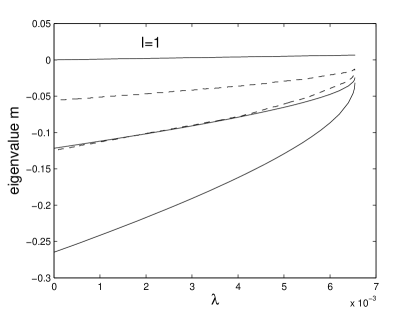
Figure 1: The eigenvalues $m$ for the three lowest-order $l=1$ p$-$modes versus $\lambda$ variation in a conventional polytropic stellar core (i.e. constant $\kappa$ or $g(x)=1$) in a homologous collapse. The upper most one is an artificial mode branch corresponding to a displacement of the coordinate origin. The lower two branches are acoustic p$-$modes with zero and one node in the radial velocity perturbation, respectively. The eigenvalues of $m$ converge to $-25\lambda_{M}/8$ in the limit of $\lambda\rightarrow\lambda_{M}$. The dashed curves represent GW results for which we have already adjusted the sign difference between eigenvalues of ours and those of GW. Our eigenvalues $m$ differ from those of GW significantly, even though the corresponding eigenfunctions agree very well with those of GW.

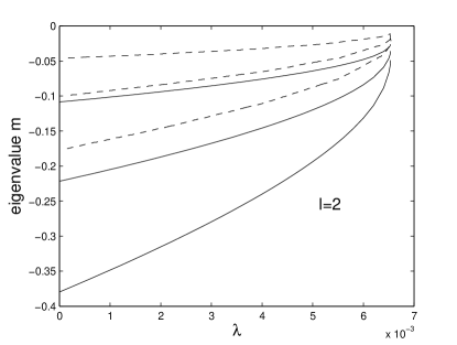
Figure 2: The three branches (solid curves) of eigenvalues $m$ for the three lowest-order $l=2$ p$-$modes versus $\lambda$ variation in a conventional polytropic stellar core (i.e. constant $\kappa$ or $g(x)=1$) in a homologous collapse. They are all eigenvalues for acoustic p$-$modes with zero, one and two nodes in the radial velocity perturbation, respectively and converge to $-25\lambda_{M}/8$ in the limit of $\lambda\rightarrow\lambda_{M}$. The dashed curves represent GW eigenvalues for which we have already adjusted the sign difference between eigenvalues of ours and GW's. Again, our eigenvalues $m$ differ from those of GW significantly, while the corresponding eigenfunctions agree very well with those of GW.

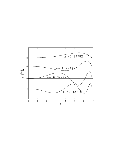
Figure 3: Acoustic p$-$mode eigenfunction profiles of our $x^{2}f^{5/4}w_{t}$ (solid curves) which is equal to $rf^{5/4}w$ (dashed curves) of GW for $l=2$ and $\lambda=0$ (i.e. the static conventional Lane-Emden sphere) are illustrated here for comparison. The eigenfunctions of GW are displayed by dashed curves; they are not readily distinguishable, because the agreements of theirs and ours are extremely close. We suspect that the eigenvalues of GW as shown in Figs. 1 and 2 are in systematic errors.

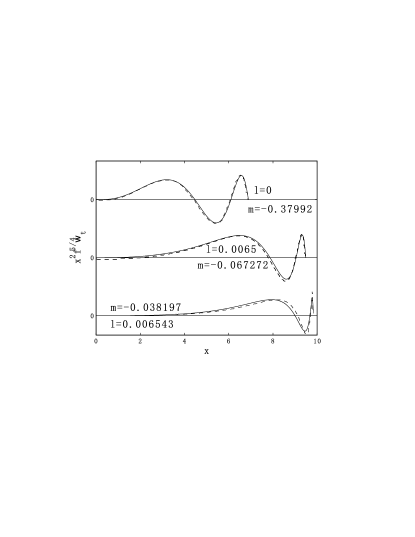
Figure 4: Here we show $l=2$ p$-$mode eigenfunctions with two radial nodes in the transverse velocity perturbation for different values of $\lambda$. These nodes concentrate towards the surface of the dynamic stellar core as $\lambda$ approaches $\lambda_{M}$. The dashed curves show GW results taken from their figure 3. Our eigenfunctions agree well with those of GW but with a considerable differences in the corresponding eigenvalues $m$ as displayed in Fig. 2.

In order to compare with GW results for acoustic perturbations in a conventional polytropic gas with $\gamma=4/3$, we simply set $g(x)=1$ and let all terms containing derivatives of $g(x)$ vanish; this simplifies perturbation ODEs (30)$-$(32) considerably. Comparing our results with those of GW, the eigenvalue curves $m(\lambda)$ for the same oscillation p$-$modes do not coincide with each other well. We have carefully checked our results in several ways and suspect systematic computational errors in the determination of eigenvalues by GW. Figs. 1 and 2 show the first three branches for eigenvalues of $m$ versus $\lambda$ for $l=1$ and $l=2$ p$-$modes (the branch with $m\;\lower 4.0pt\hbox{${\buildrel\displaystyle>\over{\sim}}$}\;0$ for $l=1$ is an exception). For visual comparisons, GW eigenvalues are also displayed by dashed curves in Figs 1 and 2. We have specifically compared the eigenfunctions of ours with those of GW in Figs. 3 and 4. Within numerical errors, the corresponding eigenfunctions agree with each other very well. We have carefully examined our computational procedures and programs and make sure that the first three eigenvalues correspond to the first three lowest-order p$-$mode oscillations with $0$, $1$ and $2$ nodes along the radial direction. We suspect systematic errors in the computational results of GW in terms of their eigenvalues.

Figs. 3 and 4 show several eigenfunctions for different eigenvalues of $m$ with specified $\lambda$ values for the background dynamic collapse. In Figs. 3 and 4, dashed curves are those of GW results. The coincidence of their curves and ours are very good. Fig. 3 shows that similar to classical non-radial oscillations of a static spherical star, the $n$th lowest eigenvalue of a p$-$mode correspond to an eigenfunction with $n-1$ number of nodes. Fig. 4 shows shape variations of eigenfunctions as $\lambda$ varies in succession. The positive $m(\lambda)$ curve in the $l=1$ case is an artificial one whose eigenfunction represents a movement of the coordinate origin. Another exceptional curve noted by GW is for the case of $l=0$, representing a different choice of the time origin. Except for these two special cases, eigenvalue $m(\lambda)$ curves of all families approach a common limit of $-25\lambda_{M}/8$ in the limit of $\lambda\rightarrow\lambda_{M}$. Curves of eigenvalue $m(\lambda)$ which are always smaller than $-25\lambda_{M}/8$ must have such a limit. Otherwise, an essential singularity of solutions appears for the limiting case of $\lambda=\lambda_{M}$ (see GW for details). Note that eigenfunctions of acoustic p$-$modes become concentrated towards the surface as $\lambda$ approaches $\lambda_{M}$. This singular behaviour of $\lambda_{M}$ should be regarded as an artifact of the special mathematical character of this limiting solution. In reality, the Lagrangian pressure perturbation vanishes at the free surface. A finite sound speed at the surface ensures that the normal modes are regular and the eigenvalues are isolated.

4.2.2 Further Numerical Explorations

With the physical requirement of $g^{\prime}(0)=0$, we consider three types of variable $g(x)$ for numerical explorations. The first type is an increasing function of $x$, the second type is a decreasing function of $x$ and the last type has both increasing and decreasing regions with increasing $x$. Referring to definition (34) of ${\cal N}^{2}$ for the buoyancy frequency squared which serves as the criterion for the existence of various g$-$modes, we find that the sign of ${\cal N}^{2}$ closely follows the sign of the first derivative of $g(x)$. Thus in order to illustrate g$-$modes under various situations, such three types of $g(x)$ are chosen as representatives. More specifically, the three forms of $g(x)$ are prescribed as even functions of $x$ and are given by

$$g(x)=1+\frac{\varepsilon_{1}x^{2}}{\varepsilon_{1}x^{2}+1}\ ,$$ (35)

$$g(x)=1-\frac{\varepsilon_{2}x^{2}}{2(\varepsilon_{2}x^{2}+1)}\ ,$$ (36)

$$g(x)=1+\varepsilon_{3}x^{2}\exp(-x^{2}/2)\ ,$$ (37)

where $\varepsilon_{1}$, $\varepsilon_{2}$, and $\varepsilon_{3}$ are three parameters calibrating the values of respective derivatives and thus the degree of variation for the dimensionless $g(x)$.

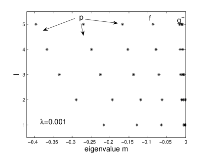
Figure 5: Eigenvalues $m$ for various oscillation modes of several lowest orders versus the angular spherical harmonic degree $l$ are shown here. Three classes of modes, namely p$-$modes, f$-$modes and g${}^{+}-$modes, are identified according to the values of $m$ and the structures of their corresponding eigenfunctions. Note that the specific entropy $g(x)$ is an increasing function of $x$ in the form of expression (35) with $\epsilon_{1}=0.01$ and parameter $\lambda=0.001$ is adopted. The g${}^{-}-$modes do not exist in this case.

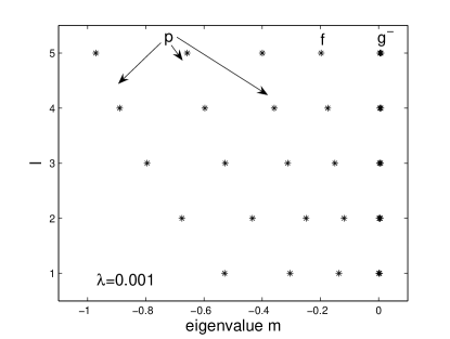
Figure 6: Eigenvalues $m$ for various oscillation modes of several lowest orders versus the angular spherical harmonic degree $l$ are shown. Three classes of modes, namely p$-$modes, f$-$mode and g${}^{-}-$modes are identified according to the values of $m$ and the structures of their corresponding eigenfunctions. Only eigenvalues $m$ of g${}^{-}-$modes are greater than zero. In this case, the specific entropy $g(x)$ is a decreasing function of $x$ in the form of expression (36) with $\epsilon_{2}=0.01$ and parameter $\lambda=0.001$ is adopted. No g${}^{+}-$modes appear in this case.

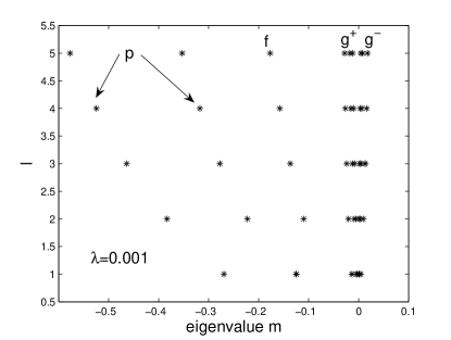
Figure 7: Eigenvalues of $m$ parameter for various oscillation modes of several lowest orders versus the angular spherical harmonic degree $l$ are shown. Four classes of perturbation modes, i.e. p$-$modes, f$-$modes, g${}^{+}-$modes and g${}^{-}-$modes, are identified according to the values of $m$. Only eigenvalues of $m$ for convectively unstable g${}^{-}-$modes are greater than zero. Here, $g(x)$ takes the form of expression (37) with $\varepsilon_{3}=0.1$, neither purely increasing nor purely decreasing, and parameter $\lambda=0.001$ is adopted.

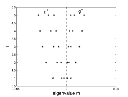
Figure 8: The enlargement of region around the ordinate axis in Fig. 7. It is clear that g${}^{+}-$modes and g${}^{-}-$modes are strictly divided by the dashed line $m=0$. The g${}^{+}-$ and g${}^{-}-$modes are distinguished according to the sign of $m$; the former corresponds to negative eigenvalues $m$ while the latter corresponds to positive eigenvalues $m$. However, the criterion for convective stability is $m<-\lambda/8$ in a dynamically collapsing stellar core rather than $m<0$ for a static background. It is therefore possible for g${}^{+}-$modes to become convectively unstable.

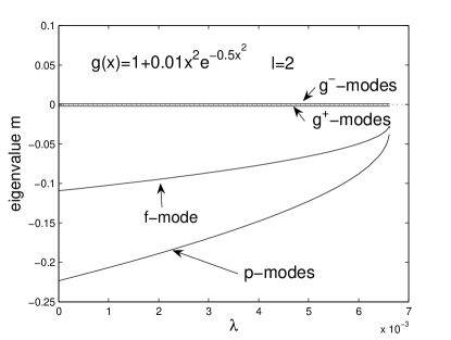
Figure 9: Examples of eigenvalues $m$ of $l=2$ p$-$modes, f$-$modes, g${}^{+}-$mode and g${}^{-}-$mode are shown in this case of $g(x)=1+0.01x^{2}\exp(-x^{2}/2)$.

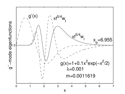
Figure 10: As an example, eigenfunctions of a convectively unstable g${}^{-}-$mode for a $g(x)$ in the form of expression (37) are shown. Relevant parameters are $\lambda=0.001$ and $l=2$ and the form of $g(x)$ is shown in the figure. The horizontal component $w_{t}$ (dashed curve) is larger than the radial component $w_{r}$ (solid curve). Here, $g^{\prime}(x)$ is shown by the dash-dotted curve. The peaks of eigenfunctions concentrate in the region of $g^{\prime}(x)<0$ corresponding to ${\cal N}^{2}<0$.

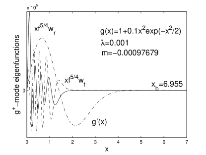
Figure 11: As another example of illustration, eigenfunctions of a stable g${}^{+}-$modes for a $g(x)$ in the form of expression (37) are shown. Relevant parameters are $\lambda=0.001$ and $l=2$ and the form of $g(x)$ is given in the figure. The horizontal component $w_{t}$ (dashed curve) is larger than the radial component $w_{r}$ (solid curve). The specific entropy $g^{\prime}(x)$ is shown by dash-dotted curve. The peaks of eigenfunctions concentrate in the central region, distinctive from g${}^{-}-$modes and p$-$modes.

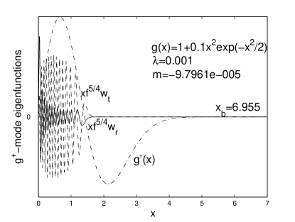
Figure 12: As the third example of illustration, unstable g${}^{+}-$modes are shown with the eigenvalue $m$ exceeding $-\lambda/8$. Relevant parameters and results are shown in the figure. It is clear that $m+\lambda/8>0$ which corresponds to an unstable mode. The dash-dotted curve is $g^{\prime}(x)$. The concentration of amplitude peaks within the region of $g^{\prime}(x)>0$, i.e. ${\cal N}^{2}>0$, and the negative value of eigenvalue $m$ both show that it is a g${}^{+}-$mode.

Several features of non-radial oscillations are contained in the spectrum of eigenvalues $m$ versus spherical harmonic degree $l$ for a given value of $\lambda$ and a prescribed form of $g(x)$. Figs. 5, 6 and 7 schematically present the mode spectra for each type of specific entropy $g(x)$ in equations (35), (36) and (37), respectively. Parameters $\varepsilon_{1}=0.01$, $\varepsilon_{2}=0.01$ and $\varepsilon_{3}=0.1$ are adopted for our numerical computations. Fig. 8 zooms in the neighborhood of the ordinate in Fig. 7. Each asterisk $*$ in the four figures represents computed eigenvalues $m$ (i.e. the abscissa) for two or three lowest order modes versus the given spherical harmonic degree $l$. As the background dynamic core collapse is spherically symmetric, 3D perturbations are degenerate with respect to the azimuthal degree $\mathfrak{m}$ (see footnote 2) as expected. Fig. 9 further illustrates the variation of $m$ versus $\lambda$ and reveals that no curve of $m(\lambda)$ goes across the line of $m=0$.

By these figures, it is clear to see the variation of eigenvalues with changing $l$. The absolute values of $m$ for p$-$modes are largest. The higher the order of a p$-$mode, the larger the absolute value of the corresponding $m$. Moreover, we find that $m$ is always smaller than $-\lambda/8$, which lead to an imaginary part in the power index of time-dependent term $\tau(t)$ for perturbations.

Eigenvalues of g$-$modes, in contrast, lie in the regime of smaller absolute value $m$, being further divided into two sub-modes according to the signs of ${\cal N}^{2}$. Figs. 5, 6 and 7 demonstrate the criteria for the existence of g${}^{-}-$modes and g${}^{+}-$modes by ${\cal N}^{2}$, the square of the Brunt-V$\ddot{\rm a}$is$\ddot{\rm a}$l$\ddot{\rm a}$ buoyancy frequency ${\cal N}$. In Fig. 5 where the form of $g(x)$ keeps ${\cal N}^{2}$ positive, only g${}^{+}-$modes exist and they are thus calculated; g${}^{-}-$modes do not exist as confirmed by our numerical explorations. In Fig. 6 where ${\cal N}^{2}$ is negative, only unstable g${}^{-}-$modes exist and they are thus calculated; g${}^{+}-$modes do not exist as confirmed by our numerical explorations. In Fig. 7 where the sign of ${\cal N}^{2}$ varies in the region, both types of g$-$modes exist and they are calculated by examples. Fig. 8 clearly shows the difference between g${}^{-}-$modes and g${}^{+}-$modes in terms of eigenvalues of $m$.

Recalling the time-dependent factor $\tau(t)$ by definitions (23) and (24) and the expression of parameter $p=-(\lambda/8)^{1/2}\pm(m+\lambda/8)^{1/2}$, we find that the criterion for convective stability changes with $\lambda$ value of a dynamic core collapse. As discussed presently, the first term $-(\lambda/8)^{1/2}$ is interpreted as the gas compression effect. Therefore for $m+\lambda/8>0$ of two real values of $\pm(m+\lambda/8)^{1/2}$, one mode decays with time $t$ while the other mode diverges with time $t$. For $m+\lambda/8<0$, both modes oscillate with time $t$. Consequently, the criterion for convective stability should be $m<-\lambda/8$ rather than simply $m<0$. The most interesting physical consequence is the appearance of unstable g${}^{+}-$modes of sufficiently high orders. Figs. 10, 11 and 12 demonstrate concrete examples of unstable $g^{-}-$modes, stable $g^{+}-$modes and unstable $g^{+}-$modes, respectively. The form of specific entropy $g(x)$ is described by expression (37) for $\epsilon_{3}=0.1$.

The unique f$-$modes (i.e. Lamb modes), shown in these figures and treated as the lowest p$-$modes, exist only for $l\geq 2$. They separate p$-$modes from g$-$modes in the sense that the eigenvalues $m$ fall between the eigenvalues of p$-$modes and those of g$-$modes. An important feature is that the eigenfunctions of f$-$modes contain no nodes in the radial component of velocity perturbation.

Non-radial oscillations of p$-$modes, f$-$modes and g$-$modes exist for $l\geq 1$ (in particular f$-$modes requires $l\geq 2$). Oscillations for $l=0$ modes are purely radial acoustic oscillations as $Y_{00}=1/(2\pi)^{1/2}$. Since the horizontal component vanishes, one can infer from the primary direction of perturbation of different modes that only p$-$modes exist. Our numerical results confirm this inference for a self-similar dynamic core collapse in that only stable p$-$modes exist for purely radial oscillations.

Moreover, several characteristic features of g$-$modes are displayed in Figs. 10, 11 and 12. These perturbations are primarily horizontal as the horizontal component of perturbation velocity is usually larger than the radial component of perturbation velocity. The peaks of g${}^{+}-$modes are trapped deeply in the stellar interior of the collapsing stellar core while peaks of g${}^{-}-$mode eigenfunctions appear in the region of ${\cal N}^{2}<0$. Both have much difference from acoustic p$-$modes in which the radial component of perturbation dominates and oscillation peaks of eigenfunctions appear towards the surface layer of a collapsing stellar core.

5 Model Considerations for SNe

Homologous collapses have been invoked here to model the dynamic phase of stellar core collapse prior to the emergence of a rebound shock and the subsequent SN explosion. In numerical simulations (e.g. Bruenn 1985) and theoretical studies (GW; Lai 2000), this phase was claimed to be stable. We perform general polytropic 3D perturbation analysis on such a homologous core collapse. Analogous to stellar oscillations of a static star, 3D perturbations during this dynamic core collapse can be classified into several distinct modes. The most interesting and important revelation is that convectively unstable g$-$modes appear under generic conditions. When this happens, several physical consequences for the remnant core follow, which may alter the scenario for the breakup of spherical symmetry during the core collapse.

5.1 Radial Evolution of Specific Entropy

In our model derivations and computations, we start from assumptions of a general polytropic gas and the self-similar collapse of such a gas sphere under self-gravity. For a homologous core collapse, we find that the general polytropic EoS is automatically satisfied. A radial evolution of specific entropy $g(x)$ needs to be prescribed for a complete solution of a homologous core collapse. Moreover, the instability of such a dynamic core collapse depends on the radial evolution of specific entropy. A brief review for the radial entropy distribution in the core collapse phase deems necessary.

According to Bethe et al. (1979), entropy per nucleon (in unit of Boltzmann's constant $k_{B}$) is $\sim 1-1.5$ at electron capture where the mean electron number per baryon $Y_{e}$ is $\sim 0.31$. This entropy value varies little such that a conventional polytropic EoS was adopted by GW. Nevertheless, Bethe et al. (1979) noted that multiple nuclear processes indeed change this value from this range and this entropy variation serves as the conceptual basis of our model. For example, when the breakup of ⁵⁶Fe occurs at a mass density of $\sim 5.9\times 10^{11}\hbox{ g cm}^{-3}$, entropy per nucleon varies from $\sim 0.5$ to $\sim 1.5$ at a temperature of $\sim 1-2$ MeV. While a constant specific entropy may be an expedient approximation, electron capture, neutrino trapping and other physical processes certainly make the specific entropy vary with position and time. It is this variation of specific entropy distribution that leads to g$-$mode convective instabilities during a stellar core collapse before the emergence of a rebound shock.

During the deleptonization process of a stellar core collapse, an entropy evolution according to numerical simulations (e.g. Bruenn 1985; Janka et al. 1995, 1996; Burrows et al. 2006) might suggest that specific entropy increases with increasing radius, as grossly described by an increasing type of $g(x)$. Bruenn (1985) displayed an increasing distribution of entropy versus the enclosed mass. As the enclosed mass always increases with radius, the specific entropy then ascends with increasing radius. More evidence comes from simulations for the evolution after the core bounce. Several models illustrate the increasing trend of specific entropy distribution with radius just after the core bounce (e.g. Janka et al. 1995, 1996; Burrows et al. 2006). If the entropy distribution varies not very much through the core bounce, then the specific entropy distribution might also be an increasing function in the core collapse stage, corresponding to an increasing trend of $g(x)$ versus $x$.

In short, the analysis of Bethe et al. (1979) indicates that entropy can vary in the core collapse phase while other numerical simulations (e.g. Bruenn 1985, 1989a, b; Janka & M$\ddot{\rm u}$ller 1995, 1996; Burrows et al. 2006, 2007b) suggested an increasing distribution of entropy during the phase of rebound shock. Therefore, the overall distribution of entropy might be assumed to increase with radius. Having said this, the possibility cannot be ruled out that in parts of regions the entropy may decrease with radius locally.

Bruenn (1985) pointed out that entropy decreases with density for mass density $\;\lower 4.0pt\hbox{${\buildrel\displaystyle<\over{\sim}}$}\;10^{12}\ {\rm g\ cm}^{-3}$. A turning point $\rho^{*}$ appears here, above which the entropy increases with density. The reason is that at a certain nuclear density, the energy level of $1f_{5/2}$ neutron shell in the nuclei becomes filled and the electron capture by nuclei is no longer allowed (e.g. Fuller et al. 1982). According to this result and the fact that mass density is a decreasing function of radius, when $\rho>\rho^{*}$ at a certain stage, the specific entropy distribution may not be a monotonic increasing function of radius. If this analysis reflects the physical reality, there are likely some regions where the specific entropy decreases with radius. Besides, detailed numerical simulations (e.g. Janka et al. 2007) with more sophisticated EoS (e.g. Hillebrandt et al. 1984; Shen et al. 1998) reveal that although the overall tendency is an outward increase, the entropy distribution may have regions where the entropy dips slightly.

The EoS and the specific entropy distribution remain open questions. No definitive evidence requires necessarily a constant or a monotonically increasing specific entropy distribution with increasing radius during the core collapse phase. By our computations, variable entropy regions certainly lead to unstable g$-$modes with possibly rapid growth rates. These findings bear important implications to perturbation growths during the core collapse prior to the emergence of a rebound shock and SN explosions.

5.2 Definition of a Collapsing Inner Stellar Core

For the type of SNe involving stellar core collapses, a rebound shock emerges surrounding the centre because the inner core is drastically compressed and stiffened obeying the EoS at nuclear density. After such a core bounce, the central neutron-rich core may become a proto-neutron star within a mass range of $\sim 1-3M_{\odot}$ (e.g. Rhoades & Ruffini 1974). One expects that in the pre-collapse stage, there should exist a dense central core with a comparable mass collapsing inwards to form such a proto-neutron star. Some numerical simulations (e.g. Woosley, Heger & Weaver 2002) give the central core masses for progenitors of various masses with different metallicities. The core mass appears in the range of $\sim 1.2-1.8M_{\odot}$ ($M_{\odot}=2\times 10^{33}$ g is the solar mass).

For a sudden core collapse, the outer layers of the progenitor may not move in immediately (Burrows 2000). As the stellar core rapidly contracts inwards, it may temporarily detach from outer shells and evolve independently. In this sense, we conceive a collapsing core under the self-gravity. Meanwhile, a quantitative definition would be desirable. GW used the invariance of the inner core mass to consider the maximum central pressure reduction percentage from a $\lambda=0$ configuration to a homologous core collapse. However, GW value of $\sim 3\%$ for the central pressure reduction is much less than the result of $\sim 26\%$ in the simulation of Bethe et al. (1979). GW defined a core mass as

$$M_{ic}=1.0449\left(\frac{\kappa_{c}}{\kappa_{c0}}\right)^{3/2}M_{0}\ ,$$

where $M_{0}$ and $\kappa_{c0}$ are the enclosed mass and the value of $\kappa_{c}$ for the $\lambda=0$ initial static Lane-Emden core while the coefficient $1.0449$ comes from the variation of $x_{b}^{3}\bar{\rho}/\rho_{c}$ as $\lambda$ varies from $0$ to the maximum value $\lambda_{M}$. GW also noted that the inner core mass in the computation of Van Riper (1978) is $\sim 30$% larger than that of their definition.

In reference to GW, we define the following inner core mass inside the iron core of the progenitor. Given a form of specific entropy evolution $g(x)$, we can determine $\lambda_{M}$ and then obtain by what factor $c_{1}$, the value of $x_{b}^{3}\bar{\rho}/\rho_{c}$ increases as $\lambda$ increases from $0$ to $\lambda_{M}$. As this inner enclosed mass $M$ is proportional to $x_{b}^{3}(\bar{\rho}/\rho_{c})\kappa_{c}^{3/2}$, if we know the value of $\kappa_{c}$ for the two cases of $\lambda=0$ and $\lambda=\lambda_{M}$, the inner core mass is then defined by

$$M_{ic}=c_{1}\left(\frac{\kappa_{c}}{\kappa_{c0}}\right)^{3/2}M_{0}\ .$$

This definition has an advantage that it allows arbitrary pressure reduction which triggers the SN explosion, though the inner core may be very small if the pressure reduction is great, especially in the GW cases of conventional polytropic EoS. In our general polytropic EoS characterized by a $g(x)$, the inner core mass can be larger according to this definition.

In our model development, we actually use parameter $\kappa_{c}$ which is the proportional coefficient between the pressure $P$ and $\rho^{4/3}$ at the centre of a collapsing core to estimate the inner core mass. According to the results shown in figure 4 of Hillebrandt et al. (1984) which gave $P$ versus $\rho$ relations for different entropies and values of the central entropy for progenitors with different metallicities (e.g. Woosley et al. 2002), we infer parameter $\kappa_{c}$ to be $\;\lower 4.0pt\hbox{${\buildrel\displaystyle>\over{\sim}}$}\;10^{14}$ cgs units. The total enclosed core mass is sensitive to the value of $\kappa_{c}$ because of the power-law dependence of $\kappa_{c}^{3/2}$. A form of specific entropy distribution $g(x)=1+0.0001x^{2}\exp{(-x^{2}/2)}$ which deviates slightly from a constant is chosen here as a demonstration. For $\kappa_{c}=3\times 10^{14}$ cgs units, the enclosed core mass does not exceed $\sim 0.7M_{\odot}$; for $\kappa_{c}=5\times 10^{14}$ cgs units, the enclosed mass is around $\sim 1.5M_{\odot}$; and for $\kappa_{c}=7\times 10^{14}$ cgs units, the enclosed core mass can reach $\sim 2.5M_{\odot}$. As expected, the central part gives the main contribution to the enclosed core mass, i.e. materials are highly concentrated around the centre. Typically, the chosen form of $g(x)$ does not change the enclosed core mass very much unless it deviates from a constant significantly.

5.3 Properties of Various Perturbation Modes

5.3.1 Stable oscillations of p$-$modes and f$-$modes

The high-frequency acoustic oscillations of p$-$modes and f$-$modes may occur in any prescribed form of $g(x)$ and are stable during the homologous core collapse. This conclusion here is more general than that of GW for a conventional polytropic stellar core collapse. In our model analysis and for convenience, f$-$modes may be regarded as the lowest-order p$-$modes. Hereafter, we do not distinguish the lowest order p$-$modes and f$-$modes unless f$-$modes are necessarily emphasized. As eigenvalues $m$ of p$-$modes decrease with increasing orders, if the lowest order mode is stable, then all acoustic p$-$modes remain stable. The local analysis in the Wentzel-Kramers-Brillouin-Jeffreys (WKBJ) approximation suggests the stability of high-order p$-$modes (GW).

A notable feature for perturbation modes in a dynamic core collapse reveals that the time-dependent factor does not take on a Fourier harmonic form $\exp(i\omega t)$ with $\omega$ being the angular frequency of a perturbation. Instead, the temporal factor acquires a power-law form, except for the limiting case of $\lambda\rightarrow 0$ which consistently reduces to the description of harmonic oscillations in a static general polytropic sphere. For stable acoustic p$-$modes, all eigenvalues $m$ found are negative and make $\lambda/8+m<0$ where $\lambda$ features the collapsing core. Therefore, the power-law index parameter $\tau(t)$ has both real and imaginary parts. The real part has a specific value of $-1/6$, corresponding to the adiabatic amplification of acoustic waves due to compression of gas collapsing towards the centre as noted by GW. The imaginary part leads to a form of $\exp(i\zeta\ln t)$ with $\zeta=\pm(-2m/\lambda-1/4)^{1/2}/3$ being a real number; this represents an oscillation, but not in a conventional sinusoidal form of harmonics.

For these oscillations of p$-$modes and f$-$modes during a dynamic core collapse, analyses of GW and ours indicate stability. If one includes effects of radiative losses and diffusive processes, then some of these acoustic oscillations may become overstable, i.e. oscillatory growths in a dynamic background. Such overstable acoustic oscillations may serve as seed acoustic fluctuations for the SASI (e.g. Foglizzo 2001) to operate during the subsequent emergence of an outgoing rebound shock (e.g. Lou & Wang 2006, 2007).

5.3.2 Perturbations of g-modes and instabilities

The most important results of our model analysis are that some g$-$modes which were used to be regarded as convectively neutral modes under the conventional polytropic approximation (GW) can become unstable in a dynamic background with a general polytropic core collapse under gravity. The occurrence of g${}^{+}-$ and g${}^{-}-$modes depends on the sign of ${\cal N}^{2}$ as highlighted in Section 4.1.

In addition to the power-law factor $t^{-1/6}$ for oscillation amplitudes by the core collapse compression, by using the modified onset criterion of convective instabilities, i.e. $m>-\lambda/8$ (see Section 4.2.2), we find that g${}^{-}-$modes and sufficiently high-order g${}^{+}-$modes are unstable during the core collapse. Here, g${}^{-}-$modes whose eigenvalues $m$ by definition are always greater than zero are unstable. Table 1 provides information of several illustrative examples of g${}^{-}-$modes; eigenvalues $m$ of g${}^{+}-$modes approach $0$ when the order goes higher. As a result, its value must exceed $-\lambda/8$ when the order is high enough. Therefore high-order g${}^{+}-$modes become unstable. Consequently, unless for a constant $g(x)$, unstable g$-$modes always exist, because at least one of the two kinds of g$-$modes occurs for a variable distribution of specific entropy.

It should be emphasized that numerical simulations so far have not shown drastic growths of unstable convective modes found here. Part of the reason is that there exists no systematic study on the stability of the core collapse. One would have thought that numerical truncation errors and errors in the determination of thermodynamic variables from a tabulated EOS are considerable. It would be highly desirable to further pursue this problem numerically.

A physical scenario is advanced below for g${}^{+}-$modes. When g${}^{-}-$modes do not occur, unstable g${}^{+}-$modes may give rise to convective instabilities during the core collapse. Initially, the inner core of a progenitor remains in a $\lambda=0$ configuration for which g${}^{+}-$modes oscillate stably. When an insufficient nuclear energy supply triggers a reduction of core pressure, the inner core begins to collapse homologously. Sufficiently high order g${}^{+}-$modes become unstable, starting to grow and break the spherical symmetry of the collapsing core. Such convective instability is limited during the core collapse because the growth rate does not exceed $t^{-1/6}\propto a^{-1/4}$ because g${}^{+}-$modes are defined by $m<0$. If the spatial scale of the core shrinks by a factor of $\sim 10^{3}$, perturbation grows by a factor of $\sim 6$. This is comparable to the compression effect of a collapsing core.

We speculate that such g$-$mode instabilities under favorable conditions might break up a collapsing core of high density and influence the formation of the central compact object and its companions, such as binary pulsars (e.g. Hulse & Taylor 1975) and planets around neutron stars (e.g. Bailes, Lyne & Shemar 1991; Wolszczan & Frail 1992).

The importance of asymmetry has been emphasized recently for the core bounce in a progenitor star prior to SN explosions. So far, one-dimensional model cannot lead to a successful SN explosion. Another consensus is that the neutrino heating mechanism alone also fails to produce a SN explosion as the energy of $\gtrsim 10^{50}\ {\rm ergs}$ appears insufficient by one or two orders of magnitude (e.g. Kirauta et al. 2006; Burrows et al. 2007a). In recent years, physical mechanisms involving two kinds of fluctuations have been proposed to effectively extract the available gravitational energy to power SN explosions. One is the SASI process, which invokes acoustic fluctuations to transfer energy. The other process relying on $l=1$ g$-$modes appears at several hundred microseconds after the core bounce as simulated by Burrows et al. (2006, 2007a, b). These two energy transfer processes destroy the spherical symmetry and make SN explosions anisotropic.

Regarding the origin of such oscillatory modes or fluctuations, our proposed instabilities which take place during the core collapse phase before the emergence of a rebound shock should have already destroyed the spherical symmetry. The condition for the occurrence of such instabilities appears generic, only requiring a variable radial specific entropy distribution. Physically, the g${}^{-}-$modes and unstable g${}^{+}-$modes lead to convections. By definition (34) for the Brunt-V$\ddot{\rm a}$is$\ddot{\rm a}$l$\ddot{\rm a}$ frequency ${\cal N}$, inequality ${\cal N}^{2}>0$ is equivalent to the Schwarzschild criterion for convective stability in a star. The global eigenfunction of a g${}^{-}-$mode describes convective motions in a homologous core collapse. For a given mode, we can calculate the time evolution of the perturbation. Table 1 gives an example of the power indices for the lowest order $l=2$ mode under the prescribed form (37) of $g(x)=1-0.1x^{2}\exp(-x^{2})$. According to Table LABEL:TB1, the power-law index varies in a wide range, allowing for both fast and slow perturbation growths, indicating the trend that instabilities go into the nonlinear regime.

Table 1: The power-law index $-[1/36+2m/(9\lambda)]^{1/2}$ in the time-dependent factor $\tau(t)$ (see eqns (23) and (24)) for the lowest order $l=2$ unstable g${}^{-}-$modes varies with $\lambda$ values for the dynamic core collapse. There are two values of $p$ resulting from one eigenvalue $m$; as the plus sign corresponds to stable modes, we only list the index of unstable modes with minus signs in calculating index $p$. In calculations of this example, we find that the decrease of eigenvalue $m$ does not exceed $0.6\%$ when $\lambda$ increases from $0$ (static core) to the maximum value $\lambda_{M}=0.00607$. The specific entropy distribution $g(x)=1-0.1x^{2}\exp(-x^{2})$ is adopted according to expression (37).

$\lambda$	$-[1/36+2m/(9\lambda)]^{1/2}$
0.001	$-1.663$
0.002	$-1.181$
0.003	$-0.969$
0.004	$-0.843$
0.005	$-0.757$
0.006	$-0.694$
$\lambda_{M}=0.00607$	$-0.690$

5.4 Comparisons with Stellar Oscillations

Apparent similarities exist in parallel between stellar oscillations of a static star and 3D general polytropic perturbations in a homologous core collapse. The classification of different oscillatory modes are introduced in reference to stellar oscillations and the degeneracy with respect to azimuthal degree $\mathfrak{m}$ is expected (see footnote 2). Acoustic p$-$modes exist for all values of perturbation degree $l$ and remain stable. The acoustic f$-$modes exist for $l\geq 2$ and also remain stable. The criterion for the existence of two different types of g$-$modes remains the same, by using the sign of the square of the Brunt-V$\ddot{\rm a}$is$\ddot{\rm a}$l$\ddot{\rm a}$ buoyancy frequency ${\cal N}^{2}$ defined by expression (34). Similar to stellar oscillations, amplitudes of g$-$modes concentrate around the core while those of p$-$modes approach the outer layer especially for high-degree $l$ acoustic oscillations. More specifically, peak amplitudes of g${}^{-}-$modes appear in the radial regions with ${\cal N}^{2}<0$.

Meanwhile, notable differences from stellar oscillations also arise in our perturbation analysis. As the most important features, the onset criterion for convective instability is modified in reference to the well-known Schwarzschild criterion. Consequently, not only g${}^{-}-$modes but also sufficiently high order g${}^{+}-$modes become unstable. We provide specific examples to demonstrate this novel phenomenon that may give rise to several possibilities to inner stellar core collapses prior to the emergence of rebound shocks and SN explosions. The time-dependent factor no longer takes the exponential form but is replaced by a power-law form.

5.5 Comparisons with Earlier Model Results

Conceptually, our perturbation analysis during the phase of stellar core collapse shows intimate connections to perturbations before the commencement of stellar core collapse and after the onset of core bounce.

Physically, the origin of perturbations can be fairly natural for massive progenitor stars. In terms of stellar evolution and dynamics, stellar oscillations of p$-$modes, f$-$modes and g$-$modes may well occur in massive stars, such as red or blue giants prior to an inner core collapse (e.g. Murphy et al. 2004). Nuclear burning in massive stars can also provide seed perturbations (e.g. Bazan & Arnett 1998; Meakin & Arnett 2006, 2007a, b). Such pre-existing stellar oscillations and perturbations associated with nuclear burning serve as sources of fluctuations during the core collapse phase before the emergence of a rebound shock around the centre.

GW studied the acoustic stability of core collapse phase for a conventional polytropic gas and noted that g$-$modes are all convectively neutral and p$-$modes are all stable. Lai (2000) extended this polytropic acoustic stability analysis to dynamic solutions of Yahil (1983) and concluded that unstable acoustic bar modes (i.e. $l=2$) exist for $\gamma\leq 1.09$. The instability is caused by an insufficient pressure against perturbations due to a soft EoS and may indicate star formation. A cloud with this instability tends to deform into an ellipsoid, in which fragmentation might occur. Except for this, no other unstable modes relevant to Yahil solutions were found in Lai's exploration. Lai also claims that Shu (1977) isothermal EWCS is unstable. In the context of Type II SNe, he stated that no destructive oscillation modes exist in the collapsing core before forming a proto-neutron star. These conclusions are based on the assumption of a conventional polytropic gas. The fact is that several nuclear processes in SN explosions most likely make specific entropy distribution variable. Then g$-$modes are no longer convectively neutral. In particular, their stability now becomes sensitive to the evolution of specific entropy. These unstable g$-$modes should play significant roles for compact remnants and SNe.

Lai (2000) analyzed and claimed the stability of Yahil (1983) solution when $\gamma\simeq 4/3$; the background dynamic flows differ from ours. Lai & Goldreich (2000) found acoustic instability growing during dynamic flows. However, their proposed instability only grows in the supersonic region where the outer envelope resides (Yahil 1983) while the core still collapses subsonically. A main assumption for these results is the same conventional polytropic EoS for background flow and perturbations. Thus g$-$modes are convectively neutral in their analysis and only acoustic p$-$modes exist.

5.6 Several Aspects of SN Explosions

One can assess consequences of g$-$mode instabilities during the phase of the core collapse prior to SNe. Such g$-$mode instabilities can grow and evolve nonlinearly and several plausible scenarios may be speculated.

In the presence of a series of core nuclear processes, including neutronization and electron capture, fluctuations in the specific entropy during the core-collapse phase is inevitable; in particular, such unstable g$-$modes, i.e. convective instabilities destroy the spherical symmetry of a collapsing core before the emergence of a rebound shock. This is a likely mechanism of producing asphericity now seemingly necessary for SN explosions. Two major consequences of such g$-$mode instabilities are as follows. (i) The formation and proper motion of a proto-neutron star can be affected. As the collapse becomes aspherical, the proto-neutron star may also become aspherical. Under favorable conditions, we speculate that such convective instabilities might be violent enough to tear a proto-neutron star into pieces. (ii) Such instabilities are expected to distort the shape of a rebound shock front. Compared with current numerical simulations, in which a rebound shock front is initially spherical, then becomes non-spherical and bends towards a particular direction where gas is driven out, our proposed non-spherical shock front at the beginning might give rise to considerable differences for these numerical simulations.

There are several conjectures if our proposed instabilities play a major role in SN explosions. The $l=1$ g$-$mode instability may give rise to kicks of proto-neutron stars. The $l=2$ instability may split the central massive core apart and implies a possible formation of binary pulsars; by adjusting the parameters in our model, we can have low-order $l=2$ g$-$mode instability in a central core whose enclosed mass is $\sim 2M_{\odot}$. High-order and high-degree g$-$mode instabilities always have a tendency to tear a central core into pieces. As a consequence, even though core collapse occurs during which neutronization is triggered and energetic neutrinos burst out, the outgoing rebound shock may leave behind a collection of broken clumps. We suggest this possibility because in observations no central compact object is found in some SN remnants, including SN1987A (Chevalier 1992; Manchester 2007; McCray 2009 private communications).

One important prediction of our proposed unstable g$-$mode convective instabilities before and during the rebound shock emergence is the resulting turbulent mixing of heavier elements in the inner layers of the core for SNe. According to the evolution theory of massive stars (e.g. Nomoto & Hashimoto 1988; Woosley & Weaver 1995), different heavy elements (e.g. Fe, Si, O, C etc.) lie in ordered core layers from inside out. Without convective instabilities occurring before the emergence of a rebound shock, these elemental layers should be more or less kept during a SN explosion. In this situation, boundaries between elemental shells are expected to be identifiable. In contrast, for our proposed g$-$mode convective instabilities, the resulting convective turbulence with sufficiently fast growths mixes elements Fe, Si, O, C in different core layers. This convective mixing mechanism of the core turbulence should bear observational consequences in detecting various heavy nuclear species and mapping their spatial distributions in SN remnants.

5.6.1 Speculations on kicks of radio pulsars

Observational evidence, including high neutron star peculiar velocities (e.g. Lyne & Lorimer 1994; Cordes et al. 1993; Burrows 2000; Arzoumanian et al. 2002; Hobbs et al. 2005), the detection of geodetic precession in the binary pulsar PSR 1913+16 (e.g. Wex et al. 2000), the spin-orbit misalignment (e.g. Kaspi et al. 1996), implies ``kick" processes by which proto-neutron stars gain considerable kinetic energies during SN explosions. Three major mechanisms have been pursued (e.g. Lai, Chernoff & Cordes 2001). Here, our proposed $l=1$ g$-$mode instabilities in a collapsing core belong to hydrodynamically driven ``kicks". We shall not dwell upon the other two, viz. electromagnetically driven ``kicks" and neutrino-magnetic field driven ``kicks".

The dipole modes of $l=1$, including p$-$modes and both types of g$-$modes, are characterized by possible displacements of the central core mass as already noted in stellar oscillations (e.g. Christensen-Dalsgaard 1976). As such dipole modes involve the core mass motion about the equilibrium centre, the core mass gains a certain amount of kinetic energy. During the violent rebound shock breakout of a SN, this core mass movement enables the remnant compact object to further gain kinetic energy and move away from the equilibrium centre. The overall centre of mass should remain fixed in space. This is a physically plausible `kick' process. Observationally, proper velocities of nascent neutron stars are typically $\sim 450\pm 90\ {\rm km\ s^{-1}}$ (e.g. Lyne & Lorimer 1994) and can reach as high as $\sim 1600\ {\rm km\ s^{-1}}$ (e.g. Cordes et al. 1993; Burrows 2000). For all perturbations with $l\neq 1$, the boundary condition at $x\rightarrow 0$ requires a zero velocity there. In these cases, the core mass and the equilibrium centre coincide. Fig. 14 offers an example of unstable $l=1$ g${}^{+}-$mode. Unstable $l=1$ g$-$modes of low orders during the core collapse phase in a massive progenitor star may give rise to the initial `kick' of a nascent proto-neutron star as joint results of nonlinear collapse evolution, rebound shock and SN explosion. Here, the requirement of low-order g$-$modes is to enclose a sufficient amount of core mass to be kicked out. Our model results indicate that with a plausible distribution of specific entropy, low-order $l=1$ g$-$modes can indeed be unstable during core collapse. Low-order g$-$modes ensures a sufficient amount of mass inside the inner most node. With such instabilities, a sizable mass in the central core can be kicked away from the equilibrium centre.

We may apply this ``kick" scenario to a plausible situation in which several physical variables are assigned typical values for a stellar core. From Hillebrandt et al. (1984) and Woosley et al. (2002), the central coefficient $\kappa_{c}$ is estimated as $\sim 5\times 10^{14}$ cgs unit. The time $t$ is characterized by the free-fall timescale $\sim(G\rho)^{-1/2}$ in the order of a few to several tens of millisecond when the mass density $\rho$ falls in the range of $\sim 10^{10}-10^{14}{\rm\ g\ cm}^{-3}$. In our model, the time $t$ is negative (i.e. time reversal) for a homologously core collapse solution; we thus take the initial time to be $-50$ ms. Here, $g(x)=1+0.001x^{2}$ represents a slight increase of specific entropy with increasing $x$. The case of $\lambda=0.006$ is close to the maximum value $\lambda_{M}$ of a physically allowed $\lambda$ and also leads to a central mass density of $\sim 10^{10}{\rm\ g\ cm}^{-3}$ consistent with simulation results (e.g. Bruenn 1985).

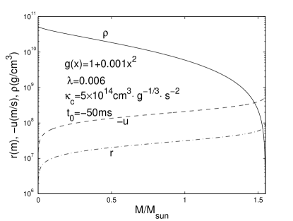
Figure 13: This example presents the initial dynamic background variables for a homologous core collapse such as the radius $r$, the collapsing velocity $-u$ and the mass density $\rho$ versus the enclosed mass $M$ in the unit of the solar mass $M_{\odot}$.

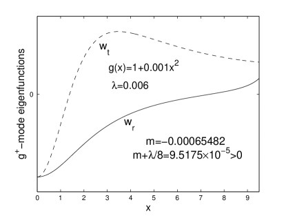
Figure 14: We show an example of the $l=1$ lowest order g${}^{+}-$mode. Parameters for this oscillatory mode are displayed in the figure. This is a convectively unstable g${}^{+}-$mode with $m+\lambda/8>0$. We can see that the centre of mass has a velocity amplitude, which contributes to the kick velocity of the core.

Fig. 13 illustrates the initial dynamic core collapse of such a situation, including the radius $r$, the collapsing velocity $-u$ and the mass density $\rho$ versus the enclosed mass $M$. Fig. 14 shows a $l=1$ dipole unstable g${}^{+}-$mode in which the central core has maximum perturbation amplitudes. It is estimated that the sound speed of the central core is $(\gamma P_{c}/\rho_{c})^{1/2}\;\lower 4.0pt\hbox{${\buildrel\displaystyle>\over{\sim}}$}\;10^{9}{\rm\ cm\ s}^{-1}$ where the subscript $c$ indicates physical variables at the centre $x=0$. For a velocity perturbation only of a few percent of the sound speed, it can still be several hundred kilometers per second which is grossly consistent with observed kick velocities of radio pulsars (e.g. Lyne & Lorimer 1994). A somewhat larger velocity perturbation amplitude (say 10% of the core sound speed) may also give rise to a kick velocity of $\sim 1600\hbox{ km s}^{-1}$ or even higher. We propose that this lower-order $l=1$ g$-$mode instability is a plausible mechanism leading to kicks of central remnant compact objects in the aftermath of SN explosions.

5.6.2 Speculations on forming binary pulsars

A few binary pulsars have been detected, including the famous PSR1913+16 (Hulse & Taylor 1975). Ideas have been proposed to explain their formation (e.g. Flannery & van den Heuvel 1975). Our $l=2$ g$-$mode instabilities suggest an alternative yet plausible origin of such binary pulsars. Unstable $l=2$ g$-$modes of low orders developed during the stellar core collapse of a massive progenitor might break the dense core apart before and during the emergence of a rebound shock and eventually give rise to binary compact objects. The violent SN explosion drives the two compact blobs apart. The spins of the two blobs and the binary orbital motion pick up part of the angular momentum of the massive progenitor star. The mass of each components in PSR1913+16 is estimated to be $\sim 1M_{\odot}$ (e.g. Flannery & van den Heuvel 1975). For a central $\kappa_{c}$ of $\sim 7\times 10^{14}$ cgs unit, the enclosed core mass can be $\;\lower 4.0pt\hbox{${\buildrel\displaystyle>\over{\sim}}$}\;2M_{\odot}$. That would be a sufficiently massive core for a possible split into two compact objects due to nonlinear evolution of unstable $l=2$ g$-$modes and subsequent core rebounce and SN explosion.

5.6.3 Speculations on breaking up neutron-rich cores

We also speculate that under possible and favorable conditions, the growth of unstable high-order high-degree (e.g. $l\geq 3$) g$-$modes and their nonlinear evolution might lead to an eventual breakup of a central proto-neutron star after the rebound shock emergence and subsequent SN explosion. In this scenario, the neutronization does occur during the brief core-collapse phase and high-energy neutrinos escape after a short moment of trapping, but without forming a coherent central neutron star in the end. The expected compact remnant is actually shredded into pieces by the nonlinear evolution of high-order and high-degree unstable convective g$-$modes. SN1987A might be such an example, for which no signals from a central compact object have ever been detected (e.g. Chevalier 1992; Manchester 2007; McCray 2009 private communications). Unstable high-order high-degree g$-$modes under other conditions might also lead to the formation of planets orbiting around a neutron star. These planets can hardly be those before the SN explosion because they can seldom survive under the expansion of the progenitor giant and the strong stellar wind as well as the SN explosion. These high-order high-degree unstable g$-$modes during the core collapse might help certain amount of gas concentrated in isolated blobs, leading to the possible formation of planets around a new-born neutron star. A few neutron stars with planets have been detected observationally (e.g. Bailes et al. 1991; Wolszczan & Frail 1992).

We have revealed and emphasized unstable growths of g$-$mode convective instabilities during the inner core collapse under self-gravity inside a massive progenitor star and speculated several physical consequences of such instabilities about central compact remnants of SNe. Together with other physical processes at different stages, such g$-$mode convective instabilities prior to the emergence of a rebound shock can be a necessary ingredient to achieve successful SN explosions. Moreover, different modes of oscillations in our classification provide sources of perturbations during the emergence of a rebound shock, for example, the $l=1$ g$-$modes discussed by Burrows et al. (2006, 2007a, b) may have well originated from our $l=1$ g${}^{+}-$ and g${}^{-}-$modes during the stellar core collapse phase before the core bounce. Nonlinear evolution of diverse initial fluctuations in various stellar core collapse conditions is expected to give rise to a diversity of possible outcomes for remnant cores of SNe.

6 Summary and Conclusions

We have systematically investigated physical properties of 3D perturbations in a hydrodynamic background of self-similar core collapse with a general polytropic EoS for a relativistically hot gas of $\gamma=4/3$, as studied in Lou & Cao (2008). For both background and perturbations, the two values of $\gamma$ are taken to be the same; the case of two different values of $\gamma$ will be explored separately. Analogous to the mode classification of stellar oscillations in a non-rotating static star (e.g. Cowling 1941), our 3D general polytropic perturbations are divided into four distinct classes of modes, viz. p$-$modes, f$-$modes, g${}^{+}-$modes (i.e. with $m<0$) and g${}^{-}-$modes (i.e. with $m>0$), according to their eigenvalue regimes of parameter $m$ in equation (25).

Stability properties of these different perturbation modes are analyzed. Similar to stellar oscillations, acoustic p$-$modes and f$-$modes remain stable for 3D general polytropic perturbations in homologous stellar core collapse. This more general conclusion also confirms the acoustic p$-$mode stabilities claimed by GW although their p$-$mode eigenvalues appear in systematic errors. The temporal amplification factor $t^{-1/6}$ in the perturbation magnitude is associated with the background gas compression during a homologous inner core collapse. In contrast, g${}^{-}-$modes and sufficiently high-order g${}^{+}-$modes are both convectively unstable modes because the onset criterion of convective instabilities is now shifted from $m>0$ for a static general polytropic sphere to $m>-\lambda/8$ for a collapsing general polytropic core where $\lambda>0$ characterizes the hydrodynamic background of a homologously collapsing stellar core. The existence of both types of g$-$modes depends on ${\cal N}^{2}$, the square of the Brunt$-$V$\ddot{\rm a}$is$\ddot{\rm a}$l$\ddot{\rm a}$ buoyancy frequency (see definition 34) which is determined by the evolution of the specific entropy distribution $g(x)$. Meanwhile, above what value of perturbation degree $l$ the g$-$modes are unstable also depends on the specific form of $g(x)$. As an example, the lowest-order $l=1$ unstable g${}^{+}-$mode is shown in Fig. 14. The peak amplitudes of g${}^{-}-$modes lie in regions of ${\cal N}^{2}<0$, which is analogous to those in stellar oscillations. These unstable g$-$modes lead to growths of convective motions in a self-similar collapsing stellar core. Their divergent growths scale as power laws in time $t$ (with $t<0$) while stable perturbation modes oscillate in the manner of $\exp(i\zeta\ln t)$.

In analyzing this perturbation problem, we also realize that the global energy criterion of Chandrasekhar (1939) is not sufficient to ensure the stability of general polytropic equilibria in view of the possible occurrence of convective instabilities for variable entropy distributions (Appendix C).

Compared to possible sources of perturbations proposed in earlier models, including the so-called ``$\epsilon-$mechanism" before the onset of inner core collapse and SASI after the core bounce, our g$-$mode convective instabilities occur during the dynamic core collapse. Contrary to earlier theoretical notions, the pre-SN stellar core collapse phase is most likely convectively unstable due to both types of g$-$mode instabilities. This is because an exactly constant specific entropy everywhere in a stellar core should be extremely rare in any realistic progenitor star (e.g. Bruenn 1985). Therefore, the spherical symmetry of a self-similar collapsing stellar core should be actually broken up earlier than presumed by most previous models of SNe.

In our scenario, oscillations of the progenitor star serve as the most natural source for 3D perturbations. For some regions of $g^{\prime}(x)<0$ leading to ${\cal N}^{2}<0$ locally, the unstable g${}^{-}-$modes, of which low-degree modes may have sufficiently fast growth rates, will soon dominate and destroy the spherical symmetry. If $g^{\prime}(x)>0$ everywhere, high-order unstable g${}^{+}-$modes will grow in a self-similar collapsing core and evolve nonlinearly.

In the presence of inevitable core g$-$mode convective instabilities, several possible consequences may follow. Most prominently, the early break-up of spherical symmetry may lead to energy concentration in particular directions and there is thus no need for a rebound shock to push against the entire outer envelope. The low-order unstable $l=1$ g$-$modes may give rise to the initial kick of a remnant central compact object. Meanwhile unstable g$-$modes correspond to the growth of convective motions which may stir up heavier elements Fe, Si, O and C in different inner layers of the collapsing core inside a massive progenitor via convective turbulence so that a mixed distribution of these elements to various extents in SN remnants is expected. This prediction of our model can be tested by nuclear abundance observations in SNe.

We further suspect that the nonlinear evolution of low-order unstable $l=2$ g$-$mode instabilities might disintegrate the central proto-neutron star core into two blobs to form binary pulsar systems under favorable conditions. Other high-order high-degree unstable g$-$modes might even prevent the formation of a coherent central compact object by breaking the core into multiple pieces. It is speculated that this might happen to supernova SN1987A without signals from a central remnant compact object. High-degree and high-order g$-$mode instabilities may lead to smaller blobs of low masses which might eventually form planets around a neutron star after a SN explosion.

Appendix A Orthogonality of Eigensolutions with Different $m$

We can now prove that eigenfunctions of different eigenvalues $m$ are mutually orthogonal. In the following illustration, superscripts ⁽¹⁾ and ⁽²⁾ are utilized to distinguish different eigenfunctions and eigenvalues. Let us proceed to evaluate the integral of

$$m^{(1)}\int f^{3}{\bf w}^{(1)}\cdot{\bf w}^{(2)}dV=-\frac{3}{4}\int\nabla\left(gf^{4}\beta_{1}^{(1)}\right)\cdot{\bf w}^{(2)}dV$$

$$+\frac{3}{4}\int f_{1}^{(1)}\nabla\left(gf^{4}\right)\cdot{\bf w}^{(2)}dV-\int f^{3}\nabla\psi^{(1)}_{1}\cdot{\bf w}^{(2)}dV\ .$$ (38)

The last term on the RHS of eq. (38) leads to

$$\!\!\!\!\!\!\!\!\!\!\!\!\!-\int f^{3}\nabla\psi^{(1)}_{1}\cdot{\bf w}^{(2)}dV=\int\psi_{1}^{(1)}\nabla\cdot\left(f^{3}{\bf w}^{(2)}\right)dV$$ (39)

$$= \!\!\!\!-\frac{1}{3}\int\psi_{1}^{(1)}\nabla^{2}\psi_{1}^{(2)}dV=\frac{1}{3}\int\nabla\psi_{1}^{(1)}\cdot\nabla\psi_{1}^{(2)}dV\ .$$

The first integration on the RHS of eq (38) can be re-expressed as

$$\frac{3}{4}\int f^{4}\left(\frac{4}{3}gf_{1}^{(1)}-\nabla g\cdot{\bf w}^{(1)}\right)\nabla\cdot{\bf w}^{(2)}dV$$ (40)

$$= -\frac{3}{4}\int f^{3}\left(\frac{4}{3}gf_{1}^{(1)}-\nabla g\cdot{\bf w}^{(1)}\right)$$

$$\qquad\qquad\times\left(ff_{1}^{(2)}+3\nabla f\cdot{\bf w}^{(2)}\right)dV$$

$$= -\int gf^{4}f_{1}^{(1)}f_{1}^{(2)}dV-3\int f^{3}gf_{1}^{(1)}\nabla f\cdot{\bf w}^{(2)}dV$$

$$+\frac{9}{4}\int f^{3}\left(\nabla f\cdot{\bf w}^{(2)}\right)\left(\nabla g\cdot{\bf w}^{(1)}\right)dV$$

$$+\frac{3}{4}\int f^{4}\left(\nabla g\cdot{\bf w}^{(1)}\right)f_{1}^{(2)}dV\ ,$$

and the second integration on the RHS of eq (38) is equal to

$$3\int f^{3}gf_{1}^{(1)}\nabla f\cdot{\bf w}^{(2)}dV+\frac{3}{4}\int f^{4}f_{1}^{(1)}\nabla g\cdot{\bf w}^{(2)}dV\ .$$ (41)

Note that both $f$ and $g$ depend only on $x$. Therefore, the result indicates that the integral

$$\int f^{3}{\bf w}^{(1)}\cdot{\bf w}^{(2)}dV$$

is manifestly symmetric in terms of superscripts ⁽¹⁾ and ⁽²⁾. Consequently, the orthogonality of eigenfunctions is proved.

Appendix B Variational Principle

The variational principle (e.g. Chandrasekhar 1964) can also be applied to this eigenvalue problem. Referring to the formula in the proof of orthogonality in Appendix A, the eigenvalue can be written as the ratio of two integrals, viz.

$$m=I_{2}/I_{1}\ ,$$ (42)

where

$$I_{1} = \int f^{3}{\bf w}^{2}dV\ ,$$ (43)

$$I_{2} = -\int gf^{4}f_{1}^{2}dV+\frac{1}{3}\int|\nabla\psi_{1}|^{2}dV$$ (44)

$$+\frac{9}{4}\int f^{3}\left(\nabla f\cdot{\bf w}\right)\left(\nabla g\cdot{\bf w}\right)dV$$

$$+\frac{3}{2}\int f^{4}f_{1}\left(\nabla g\cdot{\bf w}\right)dV\ .$$

Using the variational principle, we will show that the eigenvalue parameter $m$ has a stationary property when $I_{1}$ and $I_{2}$ are evaluated in terms of the true proper solutions. According to equation (42),

$$\delta m=\left(\delta I_{2}-m\delta I_{1}\right)/I_{1}\ ,$$ (45)

where $\delta I_{1}$ and $\delta I_{2}$ are the changes in $I_{1}$ and $I_{2}$ in response to the variation $\delta{\bf w}$ in ${\bf w}$. We have

$$\delta I_{1}=2\int f^{3}{\bf w}\cdot\delta{\bf w}dV\ ,$$ (46)

and

$$\delta I_{2}\!\!\!\!\!\! = \!\!\!\!\!\!-2\int gf^{4}f_{1}\delta f_{1}dV+\frac{2}{3}\int\nabla\psi_{1}\cdot\nabla\delta\psi_{1}dV$$ (47)

$$\!\!\!\!\!\!+\frac{3}{2}\int f^{4}\left(\nabla g\cdot{\bf w}\right)\delta f_{1}dV+\frac{3}{2}\int f^{4}f_{1}\left(\delta g\cdot\delta{\bf w}\right)dV$$

$$\!\!\!\!\!\!+\frac{9}{4}\int f^{3}\left(\nabla f\cdot\delta{\bf w}\right)\left(\nabla g\cdot{\bf w}\right)dV\ .$$

Keeping in mind of equations (25)$-$(28), we can write the variation $\delta I_{2}$ as

$$\delta I_{2}=2\int\left\{-\frac{3}{4}\left[\nabla\left(gf^{4}\beta_{1}\right)\right.\right.\qquad\qquad\qquad$$

$$\left.\left.-f_{1}\nabla\left(gf^{4}\right)\right]-f^{3}\nabla\psi_{1}\right\}\cdot\delta{\bf w}dV\ .$$ (48)

By equations (46) and (48), it then follows that $\delta m=0$ if

$$mf^{3}{\bf w}=-\frac{3}{4}\left[\nabla\left(gf^{4}\beta_{1}\right)-f_{1}\nabla\left(gf^{4}\right)\right]-f^{3}\nabla\psi_{1}\ ,$$ (49)

which is precisely equation (25) for the eigenvalue problem of our model formulation.

Appendix C  Total Energy of a
   General Lane-Emden Sphere

In the model formulation of Lou & Cao (2008), the situation of $\lambda=0$ represents the limiting static general polytropic sphere. For the conventional polytropic equation of state (i.e. a constant specific entropy everywhere independent of time $t$), the governing equation of the static equilibrium returns to the well-known Lane-Emden equation (e.g. Eddington 1926; Chandrasekhar 1939). For a general polytropic gas sphere with a variable radial distribution of the specific entropy, we refer to the governing equation with $\lambda=0$ as the general Lane-Emden equation (see footnote 1 in the main text). We emphasize that the linear stability property now depends on the radial distribution of the specific entropy. If the specific entropy decreases with radius $r$, corresponding to a decreasing $g(x)$, convectively unstable g${}^{-}-$modes will develop and drive the static sphere out of equilibrium configuration. The total energy that is equal to the gravitational energy plus the thermal energy together still remains zero for $\gamma=4/3$; however, this situation under the conventional polytropic assumption is referred to as being marginally stable by Chandrasekhar (1939).

The hydrostatic equilibrium equations are

$$\frac{dM}{dr}=4\pi r^{2}\rho\ ,$$ (50)

$$\frac{dP}{dr}=-\frac{GM\rho}{r^{2}}\ .$$ (51)

Using equation (50) to eliminate $M$ in equation (51) and assuming the radial distribution of $P/\rho^{\gamma}$, one readily arrives at the dimensional general Lane-Emden equation whose dimensionless form appears as equation (14) with $\lambda=0$.

The total energy of the system can be derived as follows. The total gravitational energy is

$$E_{G}=-\int\frac{GM\rho}{r}4\pi r^{2}dr=\int\frac{dP}{dr}4\pi r^{3}dr\$$ (52)

and the total thermal energy is

$$E_{T}=\int\frac{P}{(\gamma-1)\rho}4\pi r^{2}\rho dr=\frac{4\pi}{(\gamma-1)}\int Pr^{2}dr\ .$$ (53)

The total energy of a general Lane-Emden sphere is

$$E=E_{G}+E_{T}=-(3\gamma-4)E_{T}\ ,$$ (54)

where finite pressure at the centre and zero pressure at the stellar surface are presumed. Consequently, we prove that irrespective of the radial distribution of the specific entropy, the total energy of a general polytropic Lane-Emden sphere remains zero for $\gamma=4/3$. Evidently, this does not guarantee the linear stability of such a equilibrium configuration.

The simple total energy criterion is not enough to judge the stability of the equilibrium configuration. The statement of Chandrasekhar (1939) is only valid because the assumption of a conventional polytropic gas excludes g$-$modes, leaving them as convectively neutral. In fact, linear stability properties rely on the radial distribution of the specific entropy. For instance, we find in this paper g${}^{-}-$mode instability for a static general polytropic Lane-Emden sphere with the square of the Brunt-V$\ddot{\rm a}$is$\ddot{\rm a}$l$\ddot{\rm a}$ frequency ${\cal N}^{2}<0$ in some parts. We therefore conclude that simply using the polytropic index $\gamma$ to judge the stability property of a static sphere is not enough for a general polytropic Lane-Emden sphere. One still needs to perform a detailed linear stability analysis for such a hydrostatic equilibrium configuration.

References

- (1) Arnett W. D., Bahcall J. N., Kirshner R. P., Woosley S. E., 1989, ARA&A, 27, 629
- (2) Arzoumanian Z., Chernoff D. F., Cordes J. M., ApJ, 2002, 568, 289
- (3) Bailes M., Lyne A. G., Shemar S. L., 1991, Nat, 352, 311
- (4) Barus R., Janka H.-T., Rampp M., Kifonidis K., 2006, A&A, 457, 281
- (5) Bazan G., Arnett W. D., 1998, ApJ, 496, 316
- (6) Bethe H. E., Brown G. E., Applegate J., Lattimer J. M., 1979, Nucl. Phys., A324, 487
- (7) Bionta R. M., et al., 1987, PRL, 58, 1494
- (8) Blondin J. M., Mezzacappa A., DeMarino C., 2003, ApJ, 584, 971
- (9) Blondin J. M., Mezzacappa A., 2006, ApJ, 642, 401
- (10) Bruenn S. W., 1985, ApJ, 58, 771
- (11) Bruenn S. W., 1989a, ApJ, 340, 955
- (12) Bruenn S. W., 1989b, ApJ, 341, 385
- (13) Burrows A., 2000, Nat, 403, 727
- (14) Burrows A., Hayes J., Fryxell B. A., 1995, ApJ, 450, 830
- (15) Burrows A., Livne E., Dessart L., Ott C. D., Murphy J., 2006, ApJ, 640, 878
- (16) Burrows A., Dessart L., Ott C. D., Livne E., 2007a, Phys. Rep., 442, 23
- (17) Burrows A., Dessart L., Livne E., Ott C. D., Murphy J., 2007b, ApJ, 664, 416
- (18) Burrows C. J. et al. 1995, ApJ, 452, 680
- (19) Chandrasekhar S., 1939, An Introduction to the Study of Stellar Structure, Dover Publications, Inc., London
- (20) Chandrasekhar S., 1964, ApJ, 139, 664
- (21) Cheng A. F., 1978, ApJ, 221, 320
- (22) Chevalier R. A., 1992a, Nat, 355, 691
- (23) Chevalier R. A., 1992b, Nat, 360, 628
- (24) Christensen-Dalsgaard J., 1976, MNRAS, 174, 87
- (25) Cordes J. M., Romani R. W., Lundgren S. C., 1993, Nat, 362, 133
- (26) Cowling T. G., 1941, MNRAS, 101, 367
- (27) Cox J. P., 1976, ARA&A, 14, 247
- (28) Deubner F.-L., Gough D., 1984, ARA&A, 22, 593
- (29) Eddington A. S., 1926, The Internal Constitution of the Stars, Cambridge University Press, Cambridge
- (30) Fatuzzo M., Adams F. C., Myers P. C., 2004, ApJ, 615, 813
- (31) Flannery B. P., van den Henvel E. P. J., 1975, A&A, 39, 61
- (32) Foglizzo T., 2001, A&A, 368, 311
- (33) Fryer C. L., Warren M. S., 2002, ApJ, 574, L65
- (34) Fryer C. L., Warren M. S., 2004, ApJ, 601, 391
- (35) Fuller G. M., Fowler W. A., Newman M. J., 1982, ApJ, 252, 715
- (36) Goldreich P., Weber S. V., 1980, ApJ, 238, 991
- (37) Gupta B. D., 1978, Mathematical Physics, Vikas, Ghaziabad, India
- (38) Hansen C. J., Kawaler S. D., 1999, Stellar Interiors, Springer, New York
- (39) Harent M., Benz W., Colgate S., 1992, ApJ, 395, 642
- (40) Harent M., Benz W., Hix W. R., Fryer C. L., Colgate W., 1994, ApJ, 435, 339
- (41) Hillebrandt W., Nomoto K., Wolff R. G., 1984, A&A, 133, 175
- (42) Hirata K. et al., 1987, Phys. Rev. Lett, 58, 1490
- (43) Hobbs G., Lorimer D. R., Lyne A. G., Kramer M., 2005, MNRAS, 360, 974
- (44) Hu R. Y., Lou Y.-Q., 2009, MNRAS, 396, 878
- (45) Huang K., 1987, Statistical Mechanics, Wiley, New York
- (46) Hulse R. A., Taylor J. H., 1975, ApJ, 195, L51
- (47) Janka H.-T., Mller E., 1995, ApJ, 448, L109
- (48) Janka H.-T., Mller E., 1996, A&A, 306, 167
- (49) Janka H.-T., Langanke K., Marek A., Martnez-Pinedo G., Mller B., 2007, Phys. Rep., 442, 38
- (50) Kitaura F. S., Janka H.-T., Hillebrandt W., 2006, A&A, 450, 345
- (51) Lai D., 2000, ApJ, 540, 946
- (52) Lai D., Goldreich P., 2000, ApJ, 535, 402
- (53) Lamb H., 1932, Hydrodynamics, 6th ed. University Cambridge Press, London
- (54) Landau L. D., Lifshitz E. M., 1987, Fluid Mechanics, 2nd edn. Pergamon Press, New York
- (55) Larson R. B., 1969, MNRAS, 145, 271
- (56) Lebovitz N. R., 1965a, ApJ, 142, 229
- (57) Lebovitz N. R., 1965b, ApJ, 142, 1257
- (58) Lebovitz N. R., 1966, ApJ, 146, 946
- (59) Lou Y.-Q., 1990, ApJ, 361, 527
- (60) Lou Y.-Q., 1991, ApJ, 367, 367
- (61) Lou Y.-Q., 1995, MNRAS, 276, 769
- (62) Lou Y.-Q., 1996, Science, 272, 521
- (63) Lou Y.-Q., Cao Y., 2008, MNRAS, 384, 611
- (64) Lou Y.-Q., Shen Y., 2004, MNRAS, 348, 717
- (65) Lou Y.-Q., Wang W.-G., 2006, MNRAS, 372, 885
- (66) Lou Y.-Q., Wang W.-G., 2007, MNRAS, 378L, 54
- (67) Lyne A. G., Lorimer D. R., 1994, Nat, 369, 127
- (68) Manchester R. N., 2007, SUPERNOVA 1987A: 20 YEARS AFTER: Supernovae and Gamma-Ray Bursters. AIP Conference Proceedings, 937, 134
- (69) Meakin C. A., Arnett D., 2006, ApJ, 637, L53
- (70) Meakin C. A., Arnett D., 2007a, ApJ, 665, 690
- (71) Meakin C. A., Arnett D., 2007b, ApJ, 667, 448
- (72) Murphy J. W., Burrows A., Heger A., 2004, ApJ, 615, 460
- (73) Nomoto K., Hashimoto M., 1988, Phys. Rep., 163, 13
- (74) Penston M. V., 1969, MNRAS, 144, 425
- (75) Phukon T. C., Sarmah B. P., Phys. Rev. D, 55, 4, 1777
- (76) Rhoades C. E., Ruffini R., 1974, Phys. Rev. Lett., 32, 324
- (77) Scuflaire R., 1974, A&A, 34, 449
- (78) Shen H., Toki H., Oyamastsu K., Sumiyoshi K., 1998, Nucl. Phys. A, 637, 435
- (79) Shu F., 1977, ApJ, 214, 488
- (80) Suto Y., Silk J., 1988, ApJ, 326, 527
- (81) Unno W., Osaki Y., Ando H., Shibahashi H., 1979, Nonradial oscillations of stars, University of Tokyo Press, Tokyo
- (82) Van Riper K. A., 1978, ApJ, 221, 304
- (83) Wang L. et al., 2002, ApJ, 579, 671
- (84) Wang W.-G., Lou Y.-Q., 2007, Ap&SS, 311, 363
- (85) Weaver T. A., Zimmerman G. B., Woosley S. E., 1978, ApJ, 225, 1021
- (86) Wilkinson J. H., 1965, The Algebraic Eigenvalue Problem, Clarendon Press, Oxford
- (87) Wolszczan A., Frail D. A., 1992, Nat, 355, 142
- (88) Woosley S. E., Weaver T. A., 1986, ARA&A, 24, 205
- (89) Woosley S. E., Weaver T. A., 1995, ApJS, 101, 181
- (90) Woosley S. E., Langer N., Weaver T. A., 1993, ApJ, 411, 823
- (91) Yahil A., 1983, ApJ, 265, 1047
- (92) Yu C., Lou Y.-Q., Bian F. Y., Wu Y., 2006, MNRAS, 370, 121