Semi-realistic heterotic ${\mathbb{Z}}_{2}\times{\mathbb{Z}}_{2}$ orbifold models

Abstract

Superstring phenomenology explores classes of vacua which can reproduce the low energy data provided by the Standard Model. We consider the heterotic $E_{8}\times E_{8}$ string theory, which gives rise to four-dimensional Standard-like Models and allows for their $SO(10)$ embedding. The exploration of realistic vacua consists of finding compactifications of the heterotic string from ten to four dimensions. We investigate two different schemes of compactification: the free fermionic formulation and the orbifold construction. The relation of free fermion models to ${\mathbb{Z}}_{2}\times{\mathbb{Z}}_{2}$ orbifold compactifications implies that they produce three pairs of untwisted Higgs multiplets. In the examples presented in this dissertation we explore the removal of the extra Higgs representations by using the free fermion boundary conditions directly at the string level, rather than in the effective low energy field theory. Moreover, by employing the standard analysis of flat directions we present a quasi–realistic three generation string model in which stringent $F$– and $D$– flat solutions do not appear to exist to all orders in the superpotential. We speculate that this result is indicative of the non–existence of supersymmetric $F$– and $D$– flat solutions in this model and discuss its potential implications. By continuing our search of semi-realistic models in different string compactifications we present a simple, yet rich, set up: the orbifold. The simplest examples of orbifold compactifications generally produce a large number of families, which are clearly unappealing for experimental reasons. We show that, by choosing a non-factorisable compactification lattice, defined by skewing its standard simple roots, we decrease the total number of generations. Although we do not provide a semi-realistic model in this framework, the method represents an intermediate step to the final realisation of phenomenologically viable three generation models. Moreover, we mention other possible tools which may be applied in the search of Standard Model-like solutions. Finally, the construction of modular invariant partition functions for $E_{8}\times E_{8}$ orbifold compactifications is presented. Several interesting examples are derived with this formalism, such as the case of a ${\mathbb{Z}}_{2}\times{\mathbb{Z}}_{2}$ shift orbifold model, in order to provide a more technical approach in the construction of consistent string models.

Contents

1. Abstract
2. Acknowledgement
3. 1 Introduction
   1. 1.1 Motivation
   2. 1.2 String theory as a theory of unification
   3. 1.3 Organisation of the chapters
4. 2 Background notions on consistent perturbative superstring theories
   1. 2.1 Bosonic strings
   2. 2.2 Vertex operators and string interactions
   3. 2.3 The superstring
   4. 2.4 One loop amplitude and modular invariance
   5. 2.5 Spin structures
   6. 2.6 Partition functions of 10D superstrings
   7. 2.7 Bosonization
      1. 2.7.1 Product expansion operator
      2. 2.7.2 Free bosons and free fermions
   8. 2.8 The heterotic string
   9. 2.9 Toroidal compactifications
5. 3 Free Fermionic Models
   1. 3.1 The free fermionic formulation
      1. 3.1.1 Model building rules and physical spectrum
      2. 3.1.2 Construction of semi-realistic models
   2. 3.2 Minimal Standard Heterotic String Models
      1. 3.2.1 Yukawa Selection Mechanism
      2. 3.2.2 Higgs Doublet–Triplet Splitting
   3. 3.3 Models with reduced untwisted Higgs spectrum
      1. 3.3.1 Flat directions
   4. 3.4 Stringent flat directions
   5. 3.5 The string model with no stringent flat-directions
      1. 3.5.1 Third and Fourth Order Superpotential
      2. 3.5.2 Flat directions
6. 4 ${\mathbb{Z}}_{2}\times{\mathbb{Z}}_{2}$ orbifold constructions
   1. 4.1 Heterotic string and toroidal compactification
   2. 4.2 Orbifold construction
      1. 4.2.1 Consistency conditions
      2. 4.2.2 Generalities on the spectrum
   3. 4.3 ${\mathbb{Z}}_{2}\times{\mathbb{Z}}_{2}$ orbifold with $SO(4)^{3}$ compactification lattice
      1. 4.3.1 Analysis of the lattice
      2. 4.3.2 Introduction of Wilson lines
      3. 4.3.3 Massless Spectrum
7. 5 Construction of partition functions in heterotic $E_{8}\times E_{8}$ models
   1. 5.1 Shift orbifold
   2. 5.2 Partition function of the heterotic $E_{8}\times E_{8}$ shift orbifold superstring with ${\mathbb{Z}}_{2}$ action
      1. 5.2.1 The bosonic contribution
      2. 5.2.2 Spectrum
   3. 5.3 A string model with no gravity
   4. 5.4 Supersymmetric ${\mathbb{Z}}_{2}\times{\mathbb{Z}}_{2}$ shift orbifold model
      1. 5.4.1 Untwisted spectrum
      2. 5.4.2 Twisted sector h
      3. 5.4.3 Torus amplitudes for the right and for the left sector
      4. 5.4.4 Massless spectrum
8. 6 Conclusions
9. A
   1. A.1 $\eta$ and $\theta$-functions and modular transformations
      1. A.1.1 $SO(2n)$ characters in terms of $\theta$-functions
      2. A.1.2 Modular transformations for $SO(2n)$ characters
   2. A.2 Definition of lattice
      1. A.2.1 Definition of shifted lattices
      2. A.2.2 Proof for the transformation properties ()
   3. A.3 Expansion of $SO(2n)$ characters in powers of q
10. B
    1. B.1 Tables for two models with reduced Higgs spectrum
11. C
    1. C.1 Weight roots of $E_{6}$ representations in the twisted sector $\theta_{2}$ of the $SO(4)^{3}$ model
12. D
    1. D.1 Total amplitude contributions of the shift orbifold in eq.()
    2. D.2 Left amplitudes of ${\mathbb{Z}}_{2}\times{\mathbb{Z}}_{2}$ orbifold model in eq.()
    3. D.3 Right amplitudes of ${\mathbb{Z}}_{2}\times{\mathbb{Z}}_{2}$ orbifold model in eq.()
13. References

List of Figures

1. 1.1 Supersymmetric perturbative consistent string theories in 10 dimensions.
2. 2.1 a) closed string worldsheet. b)open string worldsheet.
3. 2.2 Mapping of the worldsheet cylinder into the complex plane. The dotted lines of constant $\tau$ are concentric circles while the lines of constant $\sigma$ follow radial directions from the origin.
4. 2.3 1)Torus diagram. 2)The flat torus as a two dimensional lattice. $a$ and $b$ represent the two non-contractible cycles of the Riemann surface.
5. 2.4 Fundamental domain.
6. 5.1 Modular transformations for a generic amplitude in orbifold models, where $a$, $b$ $\in\{{1,g,h,f}\}$ for a ${\mathbb{Z}}_{2}\times{\mathbb{Z}}_{2}$ orbifold.
7. 5.2 Modular orbits in ${\mathbb{Z}}_{2}\times{\mathbb{Z}}_{2}$ orbifolds.

Chapter 1 Introduction

1.1 Motivation

The Standard Model (SM) of Particle Physics describes correctly the physics of the elementary particles and their interactions, as confirmed by the experiments up to the electroweak scale $M_{W}=246$ GeV. It combines three of the four fundamental forces in nature, the weak, the strong and the electromagnetic interaction, into a unique theoretical framework, which is a Yang-Mills gauge theory based on the symmetry group $SU(3)_{C}\times SU(2)_{L}\times U(1)_{Y}$ ($C$, $L$ and $Y$ denote the colour, the weak isospin and the hypercharge quantum number respectively). In particular, the weak and the electromagnetic interactions are described by the $SU(2)_{L}\times U(1)_{Y}$ gauge symmetry, which is spontaneously broken to a $U(1)_{em}$ by the Higgs mechanism [1]. The resulting massive gauge bosons, $W^{\pm}$ and $Z^{0}$, mediate the weak interactions, while the massless boson $\gamma$, the photon, is the carrier of the electromagnetic force. The Quantum Chromodynamics is described by the $SU(3)_{C}$ sector, which remains unbroken, where the messengers of the strong interaction are eight massless gluons. The Standard Model content consists of three generations of leptons and three generations of quarks, in agreement with the observed experiments. The predictability of the Standard Model is a consequence of its renormalizability, which assures a consistent perturbative analysis of quantities related to the particle physics (infinities that may appear in the calculations are consistently absorbed into a finite number of physical parameters). Despite the achievements accomplished in this set up, several issues have not been resolved yet. We list below some among the most important shortcomings of the Standard Model [2].

$\bullet$ Absence of gravity: the Standard Model does not include in its description the Newtonian force, which is $42$ orders of magnitude smaller than the nuclear forces. Although General Relativity describes its infrared properties consistently, gravity is characterised by non-renormalizable operators which produce ultraviolet divergences.

$\bullet$ The hierarchy problem: the Higgs boson, responsible for the electroweak symmetry breaking and for the generations of the masses for the elementary particles, has a mass of the order of $100$ GeV (if correctly predicted by the Standard Model). This mass receives radiative corrections which can make the Higgs very heavy ($\sim 10^{19}$ GeV), while its vacuum expectation value is of the order of the electroweak scale. The hierarchy between the two energy scales in the physics of the Higgs boson appears very unnatural, and certainly unappealing for a fundamental theory. The introduction of supersymmetry (a symmetry between fermionic and bosonic degrees of freedom in the theory) solves this problem by preventing the scalar particle to acquire the dangerous contributions from the perturbation theory, thus stabilising its mass.

$\bullet$ The grand unification: the coupling constants for the electromagnetic and nuclear forces are parameters which depend on the energy scale. If their behaviour is extrapolated at high energy, roughly $10^{16}$ GeV, these values approach to one point but do not coincide. If supersymmetry is included, the final theory provides a unified description of the forces of the Standard Model at high energy.

$\bullet$ The arbitrariness: more than twenty free parameters describe the physics of the Standard Model and their values are completely arbitrary. For instance, the fermion masses, the gauge and Yukawa couplings, the Kobayashi-Maskawa parameters and many others have to be fixed by the experiments and put by hand into the theory.

There are many other open questions related to the physics of the Standard Model, such as the problem of the cosmological constant, whose small value cannot be explained in this set up. Also, the number of families does not find a reasonable explanation. Moreover, we mention the non-zero neutrino masses, due to their oscillations, which does not fit into the description of the leptonic physics of the Standard Model. The attempts of surmounting all these inconsistencies lead to several different theoretical solutions in the physics beyond the Standard Model, for instance the introduction of grand unification theories (GUTs) and supersymmetry. The main target of GUTs theories [2, 3] is solving the unification problem previously mentioned, by extending the gauge symmetry group of the SM to a $G_{GUT}$ characterised by only one gauge coupling. In principle, the strong, the weak and the electromagnetic interaction merge together at some higher energy scale $M_{GUT}$ where the theory has the larger gauge symmetry $G_{GUT}$. When the energy decreases below $M_{GUT}$ then the GUT symmetry breaks to the SM gauge group $SU(3)\times SU(2)\times U(1)$ and the couplings associated with different factors evolve at different rate. The smallest simple group which accommodates the SM is the $SU(5)$ with $M_{GUT}\simeq 10^{15}$ GeV [4]. A typical feature of grand unified theories is the mixing of quarks and leptons into the same group representation. Thus, in the case of $SU(5)$ gauge group, a matter generation is contained into the two irreducible representations $\{{\bf{10}}\,,\,{\bf{\bar{5}\}}}\in SU(5)$. By considering a larger $G_{GUT}$, for example an $SO(10)$ symmetry [5], it is possible to combine one generation into only one irreducible representation, precisely the ${\bf{16}}$ of $SO(10)$. In the last case, the presence of a singlet state, the right-handed neutrino, and the absence of exotic particles makes the model very predictive. Unfortunately, there are several unsolved questions appearing in grand unified theories, most of which originated from the quark-lepton mixing. A first example is given by the existence of new interactions that violate lepton and baryon number, which are responsible for the instability of the proton. Another typical problem is the presence of colour-triplet Higgs states which we do not expect to see in the low energy spectrum (the so-called doublet-triplet splitting problem). Additionally, the hierarchy problem, which affects already the physics of the SM, does not find a solution in GUTs theories. Finally, they still suffer from the lack of gravity.

Several answers to the previous problems are presented by supersymmetric theories. In particular the hierarchy problem is solved with the introduction of supersymmetry (SUSY), as anticipated earlier, which associates to each boson of the theory a fermionic superpartner with the same quantum numbers (since any internal symmetry commutes with SUSY). This symmetry is an extension of the Poincaré algebra which includes the fermionic generators $Q^{i}$, $i=1,..N$, satisfying anticommutation relations. The way supersymmetry overcomes the hierarchy problem is by "doubling" the spectrum, where each scalar coexists with its fermionic partner. Basically, the radiative corrections of the scalar Higgs at one-loop include a divergent scalar self-energy term. In supersymmetric theories a quadratically divergent term from the bosonic superpartner arises, giving exactly an opposite contribution. Hence, we assist to a cancellation of terms which stabilises the scalar masses of the theory. At low energies there is no experimental evidence of supersymmetric particles, implying that SUSY has to be broken at a relatively low scale, while being an exact symmetry at high energies.

1.2 String theory as a theory of unification

As mentioned before, the non-renormalizability of General Relativity makes a consistent description of quantum gravity problematic. Therefore, the formulation of a quantum theory that includes gravity and the other forces is very important. String theory seems to be the most successful candidate for a unified theory of all forces in nature, as we explain in the following. The regularization of the gravitational interactions is realised thanks to the introduction of an extended object, the string. The known particles are identified with massless excitations of the string. Beside these particles there is an infinite tower of fields with increasing masses and spins [6, 7] with typical mass of the order of the Plank scale $M_{P}\sim 10^{19}$ GeV. Among all excitation modes the graviton, the quantum of the gravitational field, arises in the spectrum, and suggests the interpretation of string theory as a quantum theory of gravity. Moreover, the presence of only one parameter (the string coupling $g_{s}$) used in the description of all phenomena, is considered a key feature in the prospective of an unifying picture. From a more technical point of view, string theory contains gauge symmetries which may incorporate the SM symmetry. Finally, supersymmetry arises in a natural way in this set up, despite the existence of consistent modular invariant string theories which are not supersymmetric. In the quantization procedure, the consistency of the string theory requires spacetime to have the critical dimension, which corresponds to $D=10$ for supersymmetric strings. In the table below we present the five 10-dimensional perturbative superstring theories and some of their most important properties.

Type	$N_{susy}$	String	Massless bosonic content
$H_{E_{8}\times E_{8}}$	1	closed and oriented	$g_{\mu\nu},\varphi,B_{\mu\nu},A_{\mu}$ of $E_{8}\times E_{8}$
$H_{SO(32)}$	1	closed and oriented	$g_{\mu\nu},\varphi,B_{\mu\nu},A_{\mu}$ of $SO(32)$
$I-SO(32)$	1	open+ closed unoriented	$g_{\mu\nu},\varphi,A_{\mu\nu},A_{\mu}$ of $SO(32)$
$IIA$	2	closed and oriented	$g_{\mu\nu},\varphi,B_{\mu\nu},C_{\mu\nu\rho},A_{\mu}$ of $U(1)$
$IIB$	2	closed and oriented	$g_{\mu\nu},\varphi,B_{\mu\nu}^{N},\varphi^{\prime},B_{\mu\nu}^{R},D_{\mu\nu\rho\sigma}^{\dagger}$

In the table above, $g_{\mu\nu},\varphi,B_{\mu\nu},A_{\mu}$ represent the graviton, the dilaton, the antisymmetric tensor and the gauge bosons respectively. The bosons $A_{\mu}$ belong to the adjoint representation of $E_{8}\times E_{8}$ or $SO(32)$ for the first three cases, while they are bosons of $U(1)$ symmetries for the type IIA case. $C_{\mu\nu\rho},\varphi^{\prime},B_{\mu\nu}^{R}$ and $D_{\mu\nu\rho\sigma}^{\dagger}$ are respectively a three-index tensor potential, a zero-form, a two-form and a four-form potential, the latter with self-dual field strength. The five superstring models are considered as different manifestations (in different regimes), of an unique theory, known as $M$-theory, and they are connected by some kind of equivalences, the so-called string dualities [8]. The underlying fundamental theory, whose low energy limit is 11 dimensional SUGRA [9], is unfortunately still poorly understood.

Figure 1.1: Supersymmetric perturbative consistent string theories in 10 dimensions.

As we can see from fig.1.1, the duality transformations relate the superstring theories in nine and ten dimensions. $T$ duality inverts the radius $R$ of the circle $S^{1}$, along which a space direction is compactified, $R\rightarrow\frac{1}{R}$. In particular, this duality relates the weak-coupling limit of a theory compactified on a space with large volume to the correspondent weak-coupling limit of another theory compactified on a small volume. $S$ duality instead provides the quantum equivalence of two theories which are perturbatively distinct. In fact, it inverts the string coupling $g_{s}\rightarrow\frac{1}{g_{s}}$. The perturbative excitations of a theory are mapped to non-perturbative excitations of the dual theory and viceversa. Fig.1.1 summarises the relevant information of the perturbative string theories and their web of dualities.

In order to make contact with the real world, the compactification of the six extra dimensions is needed. This procedure follows the Kaluza-Klein dimensional reduction of quantum field theory and is generalised to the case where a certain number of spacetime dimensions give rise to a compact manifold, invisible at low-energy [10, 11]. Demanding four-dimensional $N=1$ supersymmetric models leads us to a special choice of internal manifolds, the so-called Calabi-Yau manifolds [12]. Compactifications of this kind are characterised by some free parameters, the moduli, generally related to the size and shape of the extra dimensions. The low energy parameters often depend on these free values which spoil the predictivity of the theory. The moduli describe possible deformations of the theory and their continuous changes allow to go from one vacuum to another. So far, the problem of fixing the moduli has not been solved yet, since no fundamental principle is able to single out a unique physical vacuum. The study of Calabi-Yau manifolds is, unfortunately, fairly complicated since the computation of properties which are not of topological nature is very difficult. A simpler class of compact manifolds is given by the toroidal compactification, although the resulting theory is not chiral. Hence, combining the desirable pictures of Calabi-Yau manifolds and toroidal compactifications, we finally arrive to the orbifold construction. The orbifold seems to provide a simple framework for the realisation of $N=1$ supersymmetric models in four dimensions, with chiral particles in the spectrum.

In this thesis we discuss two main compactification schemes which offer complementary advantages in the understanding of semi-realistic heterotic string models. The first approach is the free fermionic construction, which is based on an algebraic method to build consistent string vacua directly in four dimensions. In the fermionic formalism all the worldsheet degrees of freedom, required to cancel the conformal anomaly, are given by free fermions on the string worldsheet. This set up offers a very convenient setting for experimentation of models, allowing a systematic classification of free fermion vacua and their phenomenological properties. Moreover, this set up provided the most semi-realistic models to date. On the other hand, the orbifold compactification, previously mentioned, leads to the analysis of other interesting features of heterotic models. For instance, the geometric picture provided by the orbifold construction may be instrumental for examining other questions of interest, such as the dynamical stabilisation of the moduli fields and the moduli dependence of the Yukawa couplings. The correspondence of free fermionic models [13, 14, 15] to ${\mathbb{Z}}_{2}\times{\mathbb{Z}}_{2}$ orbifold compactification is a key point of this thesis. In fact, the phenomenologically appealing properties of the free fermionic models and their relation to ${\mathbb{Z}}_{2}\times{\mathbb{Z}}_{2}$ orbifolds provide the clue that we might gain further insight into the properties of this class of quasi–realistic string compactifications by constructing ${\mathbb{Z}}_{2}\times{\mathbb{Z}}_{2}$ orbifolds on enhanced non-factorisable lattices (the point at which the internal dimensions are realised as free fermions on the worldsheet is a maximally symmetric point with an enhanced $SO(12)$ lattice, which is in principle non-factorisable).

In this thesis we produced the following results. We presented two semi-realistic models in the free fermionic formulation with a reduced Higgs spectrum. The truncation of the Higgs content is realised for the first time in this set up at the level of the string scale, by the assignment of asymmetric boundary conditions to the internal right- and left-moving fermions of the theory. Moreover, the analysis of flat directions, performed with the standard methods, leads to an unexpected result. The Fayet-Iliopoulos D-term which breaks supersymmetry perturbatively in our models is not compensate by the existence of D- and F- flat solutions, which would restore supersymmetry. The Bose-Fermi degeneracy of the spectrum implies that the models are supersymmetric at tree level. Thus, the models presented may provide a new interpretation of the supersymmetry breaking in string theory. In the framework of the orbifold construction, we built a ${\mathbb{Z}}_{2}\times{\mathbb{Z}}_{2}$ orbifold with a skewed $SO(4)^{3}$ compactification lattice and analysed its spectrum and symmetry group. Our main goal initially was reproducing a three generation free fermionic model [16] with gauge symmetry $E_{6}\times U(1)^{2}\times SO(8)^{2}_{H}$. Unfortunately we could not obtain the wished features, not even after the introduction of Wilson lines. Nevertheless, several interesting properties are discussed concerning the compactification lattice and its possible tools to realise semi-realistic four dimensional models in the construction of orbifold models. Finally, we concluded this thesis with the construction of modular invariant partition functions for heterotic shift orbifolds. In this context we presented different examples of consistent vacua with the derivation of the full perturbative spectrum. In particular, we discussed the details of a ${\mathbb{Z}}_{2}\times{\mathbb{Z}}_{2}$ shift orbifold model which contains some technical subtleties due to the elements of the orbifold group, and presented in detail its massless spectrum.

1.3 Organisation of the chapters

The topics of this thesis are organised as follows.

$\bullet$ Chapter 2

A general introduction on the bosonic and fermionic string is presented in order to provide perturbative superstring constructions. A brief overview on the partition function which encodes the modular invariant properties of the theory is discussed. We explain the bosonization procedure necessary for the correspondence between fermionic and bosonic conformal field theories. We close the chapter with some generalities on the heterotic string, which will be analysed in great detail in the next chapters.

$\bullet$ Chapter 3

We present the main features of four-dimensional semi-realistic models in the free fermionic construction and show the advantages of using this compactification scheme. We fix the formalism to provide the consistency constraints and the model building rules for this framework and explain the general derivation of the spectrum. In the second part of the chapter we present two very peculiar examples of semi-realistic free fermionic models, where the reduction of the Higgs content is, for the first time, realised at the string scale. Moreover, the standard analysis of flat directions is in both cases unable to restore supersymmetry perturbatively, although the models are supersymmetric at the classical level. This point opens new interpretations for the supersymmetry breaking mechanism in string theory.

$\bullet$ Chapter 4

We start by introducing the heterotic string in its bosonic formulation, followed by the description of the toroidal compactification. We proceed by providing the generalities of orbifold constructions. The discussion of the spectrum is initially performed at an abstract level to find in the last part of the chapter a concrete application, in the case of a ${\mathbb{Z}}_{2}\times{\mathbb{Z}}_{2}$ orbifold with $SO(4)^{3}$ compactification lattice. In our example we seize the opportunity to present the explicit derivation of the fixed tori for a non-factorisable lattice and investigate possible ways to control the number of families, for example by considering Wilson lines.

$\bullet$ Chapter 5

Some interesting examples of heterotic strings compactified on shift orbifolds are presented, providing the technical details on the derivation of ${\mathbb{Z}}_{2}$ and ${\mathbb{Z}}_{2}\times{\mathbb{Z}}_{2}$ orbifold partition functions. As an example is obtained, a consistent modular invariant string vacuum with no graviton. This model is in a way reminiscent of string vacua without gravity - "little string" models.

$\bullet$ Chapter 6

We conclude this thesis underlining the main aim of our research, the semi-realistic heterotic string constructions in different compactification schemes. We present the main results obtained and finally provide possible interesting outlooks.

Chapter 2 Background notions on consistent perturbative superstring theories

In this chapter we briefly present aspects of the perturbative formulation of string theory and introduce the necessary tools for the construction of semi-realistic four dimensional superstring models. The sources of the introductory part are given by [17, 18, 19, 20, 21, 22, 23, 24].

We start by presenting the bosonic string, which is the simplest instance of a string theory. This two-dimensional conformal theory at the classical level is consistent only at the critical dimension D=26. In its low energy spectrum, provided by the massless excitation modes, the presence of a symmetric metric tensor $g_{\mu\nu}$, the candidate of the graviton field, gives the main motivation for interpreting string theory as a quantum theory of gravity. Two main reasons make the bosonic string inadequate for a complete description of the fundamental interactions, such as the existence of tachyonic states, a sign of instability for the theory, and the absence of fermionic excitations in the perturbative spectrum. The solution to these problems leads to the introduction of the superstring, a superconformal theory with critical dimension D=10. After presenting the classical action for the bosonic and fermionic string, we will discuss the quantization procedure of the theory. The concepts of conformal invariance and modular invariance are explained in detail. We concisely mention how to calculate string interactions whilst giving a detailed overview on the partition function for the closed bosonic string, the torus amplitude, since this quantity represents one of the main topics treated in the following chapters [25, 26]. In the last section we introduce the concept of toroidal compactification which will be considered extensively in chapter 4, before the orbifold constructions of semirealistic models. In most cases we restrict our discussion to the closed strings since our target is the construction of the heterotic string.

2.1 Bosonic strings

Strings are one dimensional finite objects whose propagation in a D dimensional spacetime gives rise to a two dimensional worldsheet $X^{\mu}(\sigma,\tau)$, $\mu=0,..D-1$. In fig. 2.1 this surface is shown in both cases of free closed and free open strings. The worldsheet is parametrized by the two real independent coordinates, $\tau$ and $\sigma$, where the first variable is a time-like parameter while the second is space-like and belongs to the interval $[0,\pi]$.

Figure 2.1: a) closed string worldsheet. b)open string worldsheet.

The physics of the string is described by the Polyakov action that, in a flat Minkowski D dimensional spacetime, assumes the form [27, 28]

$$S=-\frac{T}{2}\int d^{2}\sigma\sqrt{-h}h^{\alpha\beta}\eta_{\mu\nu}\partial_{\alpha}X^{\mu}\partial_{\beta}X^{\nu},$$ (2.1)

where $T$ is the string tension, $h^{\alpha\beta}$ is the worldsheet metric and $h=det(h^{\alpha\beta})$, while $d^{2}{\sigma}$ implies the equivalent notation $\sigma=(\sigma^{0},\sigma^{1})=(\tau,\sigma)$.

For a general background we can simply replace the flat metric $\eta_{\mu\nu}$ by $g_{\mu\nu}(X)$ and eq.(2.1) becomes the worldsheet action of D dimensional scalar fields $X^{\mu}$ coupled to the dynamical two-dimensional metric (theory of quantum gravity coupled to matter).

The Polyakov action has three symmetries:

• Poincaré invariance in the target space $X^{\mu}$.

• Local reparametrization invariance.

• Conformal (Weyl) invariance.

The last two properties are local symmetries which can be used to fix the worldsheet metric in the conformal gauge, $h_{\alpha\beta}=e^{\phi(\tau,\sigma)}\eta_{\alpha\beta}$, obtaining a flat metric up to a scaling function. The equations of motion (e.o.m.) for the bosonic fields $X^{\mu}$ and for the metric $h^{\alpha\beta}$ are obtained in the usual procedure, as the variation of the action with respect to each of these fields respectively. At this point it is convenient to introduce the two-dimensional stress tensor $T_{\alpha\beta}$ which provides the constraints for the string theory. We define $T_{\alpha\beta}$ (also known as energy-momentum tensor) as the variation of the Polyakov action with respect to the world-sheet metric

$$T_{\alpha\beta}=-\frac{2}{T\sqrt{-h}}\frac{\delta S}{\delta h^{\alpha\beta}}=\partial_{\alpha}X^{\mu}\partial_{\beta}X_{\mu}-\frac{1}{2}h_{\alpha\beta}h^{\rho\gamma}\partial_{\rho}X^{\mu}\partial_{\gamma}X_{\mu},$$ (2.2)

then the request that the energy-momentum tensor vanishes,

$$T_{\alpha\beta}=0,$$ (2.3)

corresponds exactly to the e.o.m. for $h^{\alpha\beta}$. This condition is called the Virasoro constraint and represents a very important ingredient when considering the physical states of the model under consideration. The stress tensor is symmetric, traceless ($T_{\alpha\alpha}=0$), as consequence of the Weyl invariance and conserved.

It is very convenient to rewrite the Virasoro conditions in the light-cone coordinates $\sigma^{+}=\tau+\sigma$, $\sigma^{-}=\tau-\sigma$ , where $\partial_{\pm}=\frac{1}{2}(\partial_{\tau}\pm\partial_{\sigma})$. Then eq.(2.3) would simply become

$$T_{--}=\frac{1}{2}(\partial_{-}X)^{2}=0\,\,;\quad T_{++}=\frac{1}{2}(\partial_{+}X)^{2}=0\,\,;\quad T_{\pm\mp}=0.$$ (2.4)

The equations of motion for the fields $X^{\mu}$ take the form $\partial_{+}\partial_{-}X^{\mu}=0$, whose general solution can be written as the sum of a “right-moving” solution plus a “left-moving” solution,

$$X^{\mu}(\tau,\sigma)=X^{\mu}_{R}(\tau-\sigma)+X^{\mu}_{L}(\tau+\sigma).$$ (2.5)

Together with the periodicity constraint $X^{\mu}(\sigma,\tau)=X^{\mu}(\sigma+2\pi,\tau)$, eq.(2.5) leads to the mode expansion

$$X^{\mu}_{R}(\tau-\sigma) = \frac{1}{2}x^{\mu}+\alpha^{\prime}p^{\mu}(\tau-\sigma)+i\sqrt{\frac{\alpha^{\prime}}{2}}\sum_{n\neq 0}\frac{1}{n}\alpha^{\mu}_{n}e^{-2in(\tau-\sigma)},$$

$$X^{\mu}_{L}(\tau+\sigma) = \frac{1}{2}x^{\mu}+\alpha^{\prime}p^{\mu}(\tau+\sigma)+i\sqrt{\frac{\alpha^{\prime}}{2}}\sum_{n\neq 0}\frac{1}{n}\tilde{\alpha}^{\mu}_{n}e^{-2in(\tau+\sigma)},$$ (2.6)

where the Regge slope parameter $\alpha^{\prime}$ is defined in terms of the string tension as $\alpha^{\prime}=1/2\pi T$. From (2.6) we see that the classical motion of the string is described by the centre of mass position $x^{\mu}$, the momentum $p^{\mu}$ and the oscillator modes.

For later convenience we define the Virasoro operators as Fourier modes of the stress tensor, that in the right-moving sector become

$$L_{m}=\frac{T}{2}\int_{0}^{\pi}d\sigma e^{2im(\tau-\sigma)}\,\,T_{--}=\frac{1}{2}\sum_{n=-\infty}^{\infty}\alpha^{\mu}_{m-n}\cdot\alpha_{\mu n}\,\,(m\neq 0).$$

The Virasoro operators satisfy the constraints $L_{m}=0$, $\forall n\in Z$ and for the case $n=0$ we obtain the mass equation for the right oscillation modes, discussed in the following section. Moreover $\alpha^{\mu}_{0}=\sqrt{\frac{\alpha^{\prime}}{2}}p^{\mu}_{0}$. The correspondent left-moving expression $\tilde{L}_{m}$ is given by the substitutions $T_{--}\rightarrow T_{++}$, $\sigma^{-}\rightarrow\sigma^{+}$ and the complex conjugate oscillators and similar conditions to the right sector hold in the left sector as well.

Quantization of the bosonic string

The oscillators, the centre of mass position and the momentum presented in eq.(2.6) satisfy the standard commutation relations, while the Virasoro operators form the so-called Virasoro algebra. In the covariant canonical quantization procedure the previous conditions are translated into the following commutators

$$[x^{\mu},p^{\mu}] = i\eta^{\mu\nu},$$

$$\left[\alpha^{\mu}_{m},\alpha^{\nu}_{n}\right] = m\delta_{m+n}\eta^{\mu\nu},$$

$$\left[\tilde{\alpha}^{\mu}_{m},\tilde{\alpha}^{\nu}_{n}\right] = m\delta_{m+n}\eta^{\mu\nu},$$

$$\left[L_{m},L_{n}\right] = (m-n)L_{m+n}+\frac{D}{12}m(m^{2}-1)\delta_{m+n}.$$ (2.7)

The other commutators between different combination of operators are zero. The Hermiticity of $X^{\mu}$ gives $(\alpha^{\mu}_{n})^{\dagger}=\alpha^{\mu}_{-n}\,;\,(\tilde{\alpha}^{\mu}_{n})^{\dagger}=\tilde{\alpha}^{\mu}_{-n}$. $D$ represents the central charge and for the bosonic string $D=\eta^{\mu\nu}\eta_{\mu\nu}$. The same algebra holds for the left operator $\tilde{L}_{m}$. From now on, when defining properties of operators in the right sector, we will assume implicitly that analogous relations hold in the left sector. In the quantization of a classical system an ambiguity is introduced in the definition of the operators. This can be solved if we consider the corresponding normal-ordered expressions. In the case of the Virasoro operators the correct definition is given by $L_{m}=\sum_{n=-\infty}^{\infty}:\alpha^{\mu}_{m-n}\alpha_{\mu n}:$. The only term sensitive to normal ordering is $L_{0}$ where a normal ordering constant $a$ is introduced.

In the covariant quantization we obtain states with negative norm which destroy the unitarity of the theory, but we can discharge those by imposing the following constraints

$$L_{m>0}|phys\rangle=0\,\,\,,\,\,\,(L_{0}-a)|phys\rangle=0.$$ (2.8)

It has been shown that the subset of positive norm states exists only for $D\leq 26$ and $a\leq 1$ [29].

It is easier to solve the Virasoro constraints in the light-cone quantization (we have already defined the operators in terms of light-cone coordinates) where the states, obtained by solving the mass-shell equation, are always positive. But if unitarity is guaranteed in this procedure, we will need to verify the Lorentz invariance, which is not manifest. We have already mentioned that for $D=26$ and $a=1$ Lorentz invariance is preserved. $D=26$ is thus a very special choice of spacetime dimensions, called the critical dimension of the bosonic string.

We use now a residual invariance, leftover after imposing the conformal gauge, which is a reparametrization invariance up to scaling, generally defined as

$$\sigma^{\prime}_{+}\rightarrow f(\sigma_{+})\,\,\,,\,\,\,\sigma^{\prime}_{-}\rightarrow f(\sigma_{-}).$$

This invariance allows to fix the value of $X^{+}$ as follows, leading to the light cone gauge,

$$X^{+}=x^{+}+2\alpha^{\prime}p^{+}\tau.$$

The light-cone coordinates are given by $X^{\pm}=(X^{0}\pm X^{D-1})/\sqrt{2}$ and by using the Virasoro constraints we can express $X^{-}$ in terms of the transverse coordinates $X^{i}$, where $i$ takes values in the transverse directions. This means that we are left only with the transverse oscillators, while the light-cone ones are given by

$$\alpha^{-}_{n} = \frac{1}{\sqrt{2\alpha^{\prime}}p^{+}}\{\sum_{m\in Z}:\alpha^{i}_{n-m}\alpha^{i}_{m}:-2a\delta_{n0}\},$$

$$\alpha^{+}_{n} = \sqrt{\frac{\alpha^{\prime}}{2}p^{+}\delta_{n0}},$$ (2.9)

and analogous expressions hold for $\tilde{\alpha}^{\pm}_{n}$. The Virasoro constraints in the light-cone gauge define the mass-shell condition for the physical states

$$2p^{+}p^{-}=\frac{2}{\alpha^{\prime}}(L_{0}+\tilde{L}_{0}-\frac{D-12}{12})\quad;\quad L_{0}=\tilde{L}_{0}.$$ (2.10)

In the first equation of (2.10) the Riemann $\zeta$ function $\zeta(-1)=-1/12$ has been used, as a result of the divergent sums of zero-points energies due to the normal ordering $a$ of $L_{0}$ and $\tilde{L}_{0}$ [30]. The second equation in (2.10) is the level matching condition, a relation which connects the left with the right excitation modes of the closed string. This constraint has to be imposed for the consistency of every closed string model and contains an important information concerning the physical states of the model, the right and the left modes provide the same contribution to the mass of the physical states. The masses of the string excitations are obtained by the contributions of the transverse momenta, which for the right sector are provided by the formula $L_{0}=\frac{\alpha^{\prime}}{4}p^{i}p^{i}+N$. The mass operator is

$$M^{2}=\frac{2}{\alpha^{\prime}}(N+\tilde{N}-\frac{D-2}{12})$$ (2.11)

and $N=\sum_{m>0}\alpha_{-m}\cdot\alpha_{m}$. In the case at hand $D=26$, thus the first state obtained from eq.(2.11) is the ground state $|p^{\mu}\rangle$, with $N=\tilde{N}=0$. Its mass is given by $M^{2}=-4a/\alpha^{\prime}$, where $a$ takes the value $1$ for consistency, as we said before. This state is the tachyon. The first excited state is the tensor $\alpha^{i}_{-1}\tilde{\alpha}^{j}_{-1}|p^{\mu}\rangle$. If we decompose it into irreducible representations of the group $SO(24)$ we obtain a symmetric tensor $g_{\mu\nu}$ (a spin-2 particle, the graviton), the antisymmetric tensor $B_{\mu\nu}$ and a scalar $\varphi$, the dilaton.

At the next level we obtain states which are organised in representations of $SO(25)$ and which are massive.

2.2 Vertex operators and string interactions

A local unitary quantum field theory has an operator-state correspondence which associates to each field a quantum state created from the vacuum. In string theory the same correspondence is realised by mapping the worldsheet cylinder to the complex plane.

Figure 2.2: Mapping of the worldsheet cylinder into the complex plane. The dotted lines of constant $\tau$ are concentric circles while the lines of constant $\sigma$ follow radial directions from the origin.

In this context it is possible to build the so-called vertex operators which give rise to a spectrum generating algebra. By using this formalism, for instance, an incoming physical state $|phys\rangle$ in the infinite worldsheet past $(\tau=-\infty)$ is given by the insertion of a vertex operator $V(z)$ at the origin $z=0$, see fig.(2.2).

In this thesis we will not go into further details concerning the vertex operators, but it is important to stress their role in the construction of string amplitudes and in the description of strings interactions.

In quantum field theory the perturbative expansion of Feynman diagrams describes the interacting particles at well defined points. The worldline of particles in spacetime is described by propagators that meet in a vertex, singular point which is responsible for ultraviolet divergences in loop amplitudes. The string Polyakov perturbation theory is given by the sum of two-dimensional surfaces which correspond to the worldsheets. When considering all contributions of the infinite tower of massive particles of the string spectrum, the ultraviolet divergences of quantum gravity loop amplitudes cancel out. The reason why the non-renormalizability of quantum field theory is solved in string theory is because its interactions are described by smooth surfaces with no singular points. The main consequence of this property is that string interactions are completely determined by the worldsheet topology. In oriented closed strings the perturbative expansion is given by only one contribution at each order of perturbation theory. This contribution corresponds to closed orientable Riemann surfaces with increasing number of handles $h$ and the perturbative series is hence weighted by $g_{s}^{-\chi}$, where $\chi$ is the Euler character, defined as $\chi=2-2h$, while the string coupling $g_{s}$ is dynamically determined by the vacuum expectation value of the dilaton field $\varphi$, $g_{s}=e^{<\varphi>}$.

A generic string scattering amplitude is given by a path integral of the form

$$A=\int\mathcal{D}h_{\alpha\beta}\mathcal{D}X^{\mu}e^{-S_{P}}\prod_{i=1}^{n}\int_{M}d^{2}\sigma_{i}V_{\alpha_{i}},$$ (2.12)

where $h_{\alpha\beta}$ is the metric on the worldsheet $M$, $S_{P}$ is the Polyakov action and $V_{\alpha}$ is the vertex operator that describes the emission or absorption of a closed string state of type $\alpha_{i}$ from the worldsheet. The conformal invariance reduces these expressions to integrals on non-equivalent worldsheets which are described by some complex parameters, the moduli. The amplitudes in eq.(2.12) are then finite dimensional integrals over the moduli space of $M$.

2.3 The superstring

As we have mentioned at the beginning, the bosonic string suffers of two main problems: the absence of spacetime fermions (necessary for a realistic description of nature) and the presence of tachyons (sign of an incorrect identification of the vacuum). The solution to these problems leads us to the construction of the superstring. The new theory is constructed by the introduction of worldsheet supersymmetry, realised by including $D$ two-dimensional Majorana fermions $\Psi^{\mu}=(\psi_{-}^{\mu},\psi_{+}^{\mu})$, $\mu=0,..D-1,$ on the worldsheet. These fields are vectors from the spacetime point of view but when combined with appropriate boundary conditions will provide spacetime fermions. In the following we will work in the RNS (Ramond-Nevew-Schwarz) formalism [31, 32], where the GSO (Gliozzi-Scherck-Olive) projections are introduced in order to obtain supersymmetry [33]. The generalised action $S_{T}$ in the conformal gauge

$$S_{T}=-\frac{T}{2}\int d^{2}\sigma(\partial_{\alpha}X^{\mu}\partial^{\alpha}X_{\mu}-i\overline{\psi}^{\mu}\rho^{\alpha}\partial_{\alpha}\psi_{\mu})$$ (2.13)

is invariant under worldsheet global supersymmetric transformations

$$\delta_{\epsilon}X^{\mu}=\bar{\epsilon}\psi^{\mu}\quad,\quad\delta_{\epsilon}\psi^{\mu}=-i\rho^{\alpha}\partial_{\alpha}X^{\mu}\epsilon,$$

with $\epsilon$ constant spinor and $\rho^{\alpha}$, $\alpha=0,1$, Dirac matrices which can be chosen as follows

$$\rho^{0}=\left(\begin{array}[]{cc}0&-i\\ i&0\end{array}\right),\quad\rho^{1}=\left(\begin{array}[]{cc}0&i\\ i&0\end{array}\right).$$

In the light-cone coordinates the fermionic contribution of eq.(2.13) is simply

$$\psi_{-}{\partial}_{+}\psi_{-}+\psi_{+}{\partial}_{-}\psi_{+},$$ (2.14)

where the space-time index $\mu$ has been suppressed.

The equations of motion are simply the Dirac equations $\partial_{\pm}\psi_{\mp}=0$. Their solutions are of the form $\psi_{-}=\psi_{-}(\sigma_{+})$ and $\psi_{+}=\psi_{+}(\sigma_{-})$, hence we can say that $\psi_{-}$ represents the right-moving field while $\psi_{+}$ is the left-moving one. The boundary conditions arise by requiring that

$$(\psi_{+}\delta\psi_{+}+\psi_{-}\delta\psi_{-})|_{\sigma=0}^{\sigma=\pi}=0.$$ (2.15)

Equation (2.15) is satisfied if $\psi_{+}$ and $\psi_{-}$ are periodic or anti-periodic

$$\psi^{\mu}_{+}(\sigma+\pi,\tau) = \pm\psi^{\mu}_{+}(\sigma,\tau),$$

$$\psi^{\mu}_{-}(\sigma+\pi,\tau) = \pm\psi^{\mu}_{-}(\sigma,\tau).$$ (2.16)

The periodic case is called Ramond (R) boundary condition while the anti-periodic is known as Neveu Schwarz (NS). The general solution in terms of mode expansion is given by

$$\psi_{-}^{\mu}=\sum_{r}b^{\mu}_{r}e^{-2i\pi(\sigma_{-})},$$ (2.17)

for the right-moving states and an analogous expression applies for the left-movers $\psi_{+}^{\mu}$ (by replacing $\sigma_{-}$ by $\sigma_{+}$ and $b^{\mu}_{r}$ by $\tilde{b}^{\mu}_{r}$ ). As a result of the boundary conditions, the frequency $r$ is integer for R boundary conditions and half-integer for the NS case.

The Ramond boundary conditions and the integer modes will describe string states that are spacetime fermions. In fact, if we consider the fundamental state $b_{0}^{i}|0;p^{\mu}>$, we see that it is massless and degenerate, as $b_{0}$ satisfies the Clifford algebra $\{b_{0}^{i},b_{0}^{j}\}=\delta^{ij}$. This means that the Ramond vacuum is a spinor of $SO(8)$ and all the states obtained from the vacuum with the creation operators are fermionic as well. Instead the NS boundary conditions with the half-integer excitations give bosons. The fundamental state $|0;p^{\mu}>$ has negative mass (tachyon) and is a scalar. The first excited massless state $b^{i}_{-\frac{1}{2}}|0;p^{\mu}>$ is a vector of $SO(8)$ and all the states in this sector, created by half-integer modes, provide bosons.

Since the superstring is an extension of the bosonic case, it is necessary to enlarge the algebra which describes the theory. Thus, the classical Virasoro constraints are now generalised to

$$J_{\pm}=0\quad,\quad T_{\pm\pm}=0,$$ (2.18)

where the supercurrents and the energy-momentum tensors are given in their light-cone gauge coordinates

$$J_{+}=\psi^{\mu}_{+}\partial_{+}X_{\mu},\quad T_{++}=\partial_{+}X^{\mu}\partial_{+}X_{\mu}+\frac{i}{2}\psi_{+}^{\mu}\partial_{+}\psi_{+\mu},$$

$$J_{-}=\psi^{\mu}_{-}\partial_{-}X_{\mu},\quad T_{--}=\partial_{-}X^{\mu}\partial_{-}X_{\mu}+\frac{i}{2}\psi_{-}^{\mu}\partial_{-}\psi_{-\mu}.$$

Quantization of the superstring

The quantization of the fermionic fields is obtained by imposing the anticommutation relations

$$\{b_{r}^{\mu},b_{s}^{\nu}\}=\eta^{\mu\nu}\delta_{r+s}\quad,\quad\{\tilde{b}_{r}^{\mu},\tilde{b}_{s}^{\nu}\}=\eta^{\mu\nu}\delta_{r+s}.$$

The anticommutator of left and right oscillators vanishes. For $r<0$ ($r>0$) $b_{r}$ denotes creation (annihilation) operators. The complete spectrum is provided by the action of the creation operators on the vacuum.

The mass-shell condition in eq.(2.11) is now generalised by redefining $N$ as the number of right bosonic plus right fermionic oscillators acting on the vacuum. Same redefinition applies to $\tilde{N}$. We have to take into account that fermions can assume R or NS boundary conditions and this will change the contribution to the zero point energy $a$. Each fermionic coordinate contributes with a $-1/48$ in the NS sector and $1/24$ in the R sector, while each boson gives a contribution of $-1/24$. In $D$ dimensions, if we are in the light-cone gauge, we have $D-2$ transverse bosons and $D-2$ transverse fermions which give $a=0$ in the Ramond sector while $a=-1/16(D-2)$ in the Neveu-Schwarz.

After quantizing the supersymmetric theory, the Virasoro constraints become

$$\left[L_{m},L_{n}\right] = (m-n)L_{m+n}+\frac{D}{8}m(m^{2}-1)\delta_{m+n},$$

$$\left[L_{m},G_{r}\right] = (\frac{m}{2}-r)G_{m+r},$$

$$\{G_{r},G_{s}\} = 2L_{r+s}+\frac{D}{2}(r^{2}-\frac{a}{2})\delta_{r+s},$$ (2.19)

where the operators are defined by their normal ordered expressions

$$L_{m} = L_{m}^{a^{\prime}}+L_{m}^{b^{\prime}},$$

$$L_{m}^{a^{\prime}} = \frac{1}{2}\sum_{n\in Z}:\alpha_{-n}\cdot\alpha_{m+n}:,$$

$$L_{m}^{b^{\prime}} = \frac{1}{2}\sum_{n\in Z+a}:(r-\frac{m}{2})b_{m-r}\cdot b_{r}:,$$

$$\ G_{r} = \sum_{n\in Z}:b_{r-n}\cdot\alpha_{n}:.$$ (2.20)

For completeness with respect to the bosonic case, we shall provide the light-cone quantization for the superstring case. The theory is ghost-free but not explicitly covariant, but we can assure Lorentz invariance if $D=10$ and $a=1/2$ [17].

The gauge is fixed with the relation $\psi^{+}=0$ and $X^{+}=\alpha^{\prime}p^{+}\tau$ and since we are fixing the longitudinal oscillator modes, the only independent degrees of freedom are the transverse ones.

A supersymmetric non-tachyonic theory is obtained when the spectrum is truncated by some GSO (Gliozzi, Scherk and Olive) projections [34]. We will explain this truncation separately in the NS and in the R sector. In the Neveu-Schwarz sector the GSO projections $P_{GSO}$ is defined by keeping states with an odd number of $b^{i}_{-r}$ oscillator excitations and removing those with even number. We define below the projection operator in the NS sector and the fermion number,

$$P^{NS}_{GSO}=\frac{1}{2}(1-(-1)^{F})\,\,,\,\,F=\sum_{r=1/2}^{\infty}b^{i}_{-r}\cdot b^{i}_{r}.$$

Thus, the bosonic ground state is now massless and the spectrum no longer contains a tachyon (which has fermion number $F=0$). In the Ramond sector, the fundamental state (a Majorana spinor) lives in the spinorial representation of $SO(8)$, as mentioned before. If we introduce the projector operator

$$P_{GSO}^{R}=\frac{1}{2}(1+(-1)^{F}\Gamma_{9}),$$

where $\Gamma_{9}=b_{0}^{1}\cdot\cdot b_{0}^{8}$ is the chiral operator in the transverse dimensions, then the fundamental state becomes a Majorana-Weyl spinor of definite chirality. $P_{GSO}^{R}$, while projecting onto spinors of opposite chirality, guarantees spacetime supersymmetry of the physical superstring spectrum (we note that the choice of sign of $(-1)^{F}\Gamma_{9}=\pm 1$, corresponding to different chirality projections on the spinors, is a matter of convention).

The general procedure to obtain the massless spectrum is to solve the massless equations for right and left sector, apply level matching condition and the particular GSO projections depending on the perturbative superstring model considered, finally tensor the left with the right states. If we want to proceed with the explicit calculation of the spectrum we need to specify the string theory we want to analyse. Supersymmetric theories with only closed strings are type IIA, type IIB and heterotic models. For type IIA and type IIB (where supersymmetry is realised in the left and right sector), by taking the tensor products of right and left movers we get four distinct sectors: NS-NS, R-R, NS-R, RN-R, where the first two sets give bosons and the last two sectors provide fermion fields in the target space. The features and differences among these two models have been given in the introduction. In this thesis we are interested in the heterotic string hence we will focus on the technicalities concerning the heterotic case starting from section 2.8.

2.4 One loop amplitude and modular invariance

The one loop vacuum amplitude, also known as genus-one partition function, represents a fundamental quantity of the theory since it encodes the full perturbative spectrum. Differently from quantum field theory, in the string theory this is a finite quantity that makes the theory modular invariant. The modular invariant constraints are in fact derived from the calculation of the one-loop vacuum amplitude. The Feynman diagram, which describes a closed string propagating in time and returning to its initial state, is a donut-shaped surface, equivalent to a two-dimensional torus.

Figure 2.3: 1)Torus diagram. 2)The flat torus as a two dimensional lattice. $a$ and $b$ represent the two non-contractible cycles of the Riemann surface.

We can parametrize the torus by a complex parameter $\tau=\tau_{1}+i\tau_{2}$ , $\tau_{2}>0$. If we define in the complex plane a lattice by identifying $z=z+1$ , $z=z+\tau$, then the torus is obtained by identifying the opposite sides of this parallelogram (see fig.2.3).

The full family of equivalent tori is obtained by the transformations

$$S:\tau\rightarrow-\frac{1}{\tau}\quad,\quad T:\tau\rightarrow\tau+1\quad,$$ (2.21)

that are the generators of the modular invariant group, whose most general transformation is given by

$$\tau\rightarrow\frac{a\tau+b}{c\tau+d}\quad ad-bc=1\quad a,b,c,d\in{\mathbb{Z}}.$$ (2.22)

The formula (2.22) generates the modular group $PSL(2,{\mathbb{Z}})$. The non-equivalent tori are contained in the so-called fundamental region

$$\mathcal{F}={\mathbb{C}}^{1}/PSL(2,{\mathbb{Z}})=\{|\tau|\geq 1\,,\,-\frac{1}{2}\leq\tau_{1}<\frac{1}{2}\,,\,\tau_{2}>0\}\,$$

(see fig.2.4). Any point outside the modular domain can be mapped by a modular transformation inside $\mathcal{F}$.

Figure 2.4: Fundamental domain.

We calculate now the vacuum amplitude for the bosonic string in analogy with the quantum field theory approach. In the case of a single scalar particle the vacuum energy $\Gamma$ is defined by the path integral

$$e^{-\Gamma}=\int\mathcal{D}\,\phi e^{-S},$$ (2.23)

where $S$ is the action of the boson in $D$ dimensions. If we want to make explicit the dependence of the integral on the particle mass $M$ we can rewrite it in terms of the Schwinger parameter $t$ and eq.(2.23) assumes the form

$$\Gamma=-\frac{V}{2}\int_{\epsilon}^{\infty}\frac{dt}{t}e^{-tM^{2}}\int\frac{d^{D}p}{(2\pi)^{D}}e^{-tp^{2}},$$ (2.24)

where $V$ is the volume of the spacetime and $p$ the momentum of the particle. The parameter $\epsilon$ is an ultraviolet cutoff that will disappear when we restrict the integration region to the fundamental region of the torus. If we calculate the Gaussian momentum integral and generalise formula (2.24) for bosonic and/or fermionic fields then we obtain

$$\Gamma=-\frac{V}{2(4\pi)^{D/2}}\int_{\epsilon}^{\infty}\frac{dt}{t^{D/2+1}}Str(e^{-tM^{2}}),$$ (2.25)

where the Supertrace $Str$ takes into account the Bose-Fermi statistics.

Let us now consider the case of the bosonic string for which we want to derive the one-loop amplitude. For the bosonic theory we have $D=26$ and $M^{2}=\frac{2}{\alpha^{\prime}}(L_{o}+\tilde{L}_{o}-2)$. At this point we need to take into account the level matching condition that can be implemented by a constraint given in terms of a real variable $s$. Subsequently, we rearrange the $t$ and $s$ parameters in the new complex "Schwinger" parameter $\tau=\tau_{1}+i\tau_{2}=s+i\frac{t}{\alpha^{\prime}\pi}$. Since the closed string sweeps a torus at one loop then we identify $\tau$ as the Teichmuller parameter parametrizing the torus (see for example [25]).

Defining $q=e^{2i\pi\tau}$ and $\overline{q}=e^{-2i\pi\overline{\tau}}$ and calculating the integral in the fundamental domain gives the partition function of the torus amplitude

$$\mathcal{T}=\int_{\mathcal{F}}\frac{d^{2}\tau}{\tau_{2}^{2}}\frac{1}{\tau_{2}^{12}}trq^{L_{0}-1}\overline{q}^{\tilde{L}_{0}-1}.$$ (2.26)

The same expression can be obtained by some geometric considerations. A point on the string propagates in the time direction as $2\pi\tau_{2}$ and in space as $2\pi\tau_{1}$. The time translation is given by the Hamiltonian $H=L_{0}+\tilde{L}_{0}-2$ and the shift along the string is given by the momentum operator $P=L_{0}-\tilde{L}_{0}$. The path integral is then

$$\mathcal{T}\propto tr(e^{-2\pi\tau_{2}H}e^{2i\pi\tau_{1}P})\sim tr(q^{L_{0}-1}\overline{q}^{\tilde{L}_{0}-1}).$$

The expansion of the operator $L_{0}$ and the calculation of the trace will transform equation (2.26) into

$$\mathcal{T}=\int_{\mathcal{F}}\frac{d^{2}\tau}{\tau_{2}^{2}}\frac{1}{\tau_{2}^{12}}\frac{1}{|\eta(\tau)|^{48}},$$ (2.27)

where the Dedekind $\eta$ function is defined in Appendix A, as well as its properties under modular transformations. Each bosonic mode then gives a contribution to the partition function equal to $\frac{1}{|\eta|^{2}}$. The integrand of eq.(2.27) is modular invariant, as we can prove by using the formulae in Appendix A.

2.5 Spin structures

When we consider the parallel transport properties of spinors on a two dimensional surface, for example on the torus, we need to introduce the so-called spin structures. They provide the fermionic contributions to the partition function and have to be defined in both Ramond and Neveu-Schwarz sectors. Some kind of GSO projections enter in the game to ensure the consistency of the theory.

A fermion moving around the two non-contractible loops of the torus gives rise to four possible spin structures, indicated as following: $A^{(++)}(\tau)$, $A^{(+-)}(\tau)$, $A^{(-+)}(\tau)$ and $A^{(--)}(\tau)$. The first entry in the exponent represents the boundary condition in the $\sigma^{1}$ direction while the second gives the boundary condition in time direction $\sigma^{0}$. The $"+"$ and $"-"$ signs label the Ramond and Nevew-Schwarz boundary conditions respectively. For brevity we focus our discussion on the spin structures of the right sector of the string.

The NS sector provides states with anti-periodic boundary conditions in the $\sigma$ direction and if we implement the periodicity in the time direction we will need to introduce the Klein operator $(-1)^{F}$ in the trace. The fermionic contributions to the path integral are given, in the R and NS sector Hilbert space, by the following expressions

$$A^{(+-)} \sim Tr_{R}(e^{-2\pi\tau_{2}H})\quad\,\,\,,\,\,A^{(++)}\sim Tr_{R}((-1)^{F}e^{-2\pi\tau_{2}H}),$$

$$A^{(--)} \sim Tr_{NS}(e^{-2\pi\tau_{2}H})\quad,\,A^{(-+)}\sim Tr_{NS}((-1)^{F}e^{-2\pi\tau_{2}H}).$$ (2.28)

The modular transformations change the boundary conditions, thus it is possible to obtain a spin structure from another by applying T and S transformations. We note that $A^{(++)}$ is modular invariant while for the other expressions the following relations hold $A^{(+-)}\,\,\,\,\underrightarrow{S}\,\,\,\,A^{(-+)}\,\,\,\,\underrightarrow{T}\,\,\,\,A^{(--)}.$ Each of these contributions is multiplied by a phase which can be derived by imposing modular invariance of the total partition function of the model under consideration. A detailed explanation on the derivation of the phases can be found in [20].

The one-loop modular invariant partition function for the right-moving sector is given by

$$Z=\frac{1}{2}Tr_{NS}[(1-(-1)^{F})q^{L_{0}-\frac{1}{2}}]+\frac{1}{2}Tr_{R}[(1+(-1)^{F})q^{L_{0}}].$$ (2.29)

The total superstring amplitude is obtained by combining eq.(2.29) with the left-moving fermionic contribution and multiply the whole expression by the bosonic part.

If we calculate the traces in eqs.(2.28) we can rewrite the spin structures in terms of the Jacobi $\theta$-functions

$$A^{(++)} = 16q^{1/3}\prod_{n=1}^{\infty}(1-q^{n})^{8}=\frac{\theta_{1}^{4}(0|\tau)}{\eta^{4}(\tau)},$$

$$A^{(+-)} = 16q^{1/3}\prod_{n=1}^{\infty}(1+q^{n})^{8}=\frac{\theta_{2}^{4}(0|\tau)}{\eta^{4}(\tau)},$$

$$A^{(--)} = q^{-1/3}\prod_{n=1}^{\infty}(1+q^{n+1/2})^{8}=\frac{\theta_{3}^{4}(0|\tau)}{\eta^{4}(\tau)},$$

$$A^{(-+)} = q^{-1/3}\prod_{n=1}^{\infty}(1-q^{n-1/2})^{8}=\frac{\theta_{4}^{4}(0|\tau)}{\eta^{4}(\tau)}.$$ (2.30)

Eq.(2.29) corresponds to the famous Jacobi identity

$$\theta_{4}^{4}-\theta_{3}^{4}-\theta_{2}^{4}=0,$$

which tells us that the superstring amplitude vanishes. The meaning of the previous result is that the contribution of NS spacetime bosons and R fermions is the same (but the two contributions have opposite statistics). This is considered an indication of supersymmetry. The general definition of $\theta$-functions as Gaussian sums and in product representations are given in Appendix A, along with their modular transformation properties.

2.6 Partition functions of 10D superstrings

In this section we present the partition function for the five perturbative superstring theories and the case of the heterotic $E_{8}\times E_{8}$ string with orbifold actions will be discussed widely in the chapter 5. A very convenient and compact way of writing the fermionic contributions (in the previous section they were given in terms of $\theta$-functions) is by defining the characters $O_{2n},V_{2n},S_{2n}$ and $C_{2n}$, representations of the $SO(2n)$ group. Their general definitions and modular transformations are presented in Appendix A. Here we give as an example the characters of the little group $SO(8)$

$$O_{8}=\frac{\theta^{4}_{3}+\theta^{4}_{4}}{2\eta^{4}} ,\quad V_{8}=\frac{\theta^{4}_{3}-\theta^{4}_{4}}{2\eta^{4}},$$

$$S_{8}=\frac{\theta^{4}_{2}+\theta^{4}_{1}}{2\eta^{4}} ,\quad C_{8}=\frac{\theta^{4}_{2}-\theta^{4}_{1}}{2\eta^{4}}.$$ (2.31)

Each definition in eqs.(2.31) represents a conjugacy class of the $SO(8)$ group, in particular, $O_{8}$ is the scalar representation, $V_{8}$ the vectorial, $S_{8}$ and $C_{8}$ are spinors with opposite chirality. The characters $V_{8}$ and $O_{8}$ provide a decomposition of the NS sector, while the $C_{8}$ and $S_{8}$ give the R spectrum. We are finally ready to present the partition functions for the $10D$ spectra of type II and type 0

$$\mathcal{T}_{IIA} = (\overline{V}_{8}-\overline{C}_{8})|(V_{8}-S_{8})|,\quad\mathcal{T}_{0A}=|O_{8}|^{2}+|V_{8}|^{2}+\overline{C}_{8}|S_{8}|+\overline{S}_{8}|C_{8}|,$$

$$\mathcal{T}_{IIB} = |V_{8}-S_{8}|^{2},\quad\quad\quad\,\,\,\,\,\,\,\,\,\,\,\quad\mathcal{T}_{0B}=|O_{8}|^{2}+|V_{8}|^{2}+|S_{8}|^{2}+|C_{8}|^{2}.$$ (2.32)

The spectrum can be read by expanding the characters in powers of $q$ and $\bar{q}$, as indicated in Appendix B.

For the heterotic case we need to introduce $SO(16)$ and $SO(32)$ characters in the partition function, in order to include the gauge degrees of freedom of the theory. The only two supersymmetric modular invariant heterotic models in 10 dimensions are those where the $E_{8}\times E_{8}$ and the $Spin(32)$ symmetries are realised and their torus amplitude is respectively

$$\mathcal{T}_{E_{8}\times E_{8}} = (\overline{V}_{8}-\overline{S}_{8})(O_{16}+S_{16})(O_{16}+S_{16})$$

$$\mathcal{T}_{S_{32}} = (\overline{V}_{8}-\overline{S}_{8})(O_{32}+S_{32}).$$ (2.33)

2.7 Bosonization

In this section we present the equivalence between fermionic and bosonic conformal field theories in two dimensions, a correspondence which allows the consistent construction of free fermionic models.

Before entering into the details we will give the definition of operator product expansions (OPEs) in conformal theories in two dimensions.

2.7.1 Product expansion operator

In quantum field theory, the infinitesimal conformal transformations

$$z\rightarrow z+\epsilon(z)\quad,\quad\bar{z}\rightarrow\bar{z}+\bar{\epsilon}(\bar{z})$$

produce a variation of a field $\Phi(z,\bar{z})$ given by the equal time commutator with the conserved charge $Q=\frac{1}{2\pi i}\oint(dzT(z)\epsilon(z)+d\bar{z}\bar{T}(\bar{z})\bar{\epsilon}(\bar{z}))$, where $T$ and $\bar{T}$ are the stress-energy tensors in complex coordinates. The products of the operators is well defined only if time-ordered. The radial quantization introduced in section 2.2 is an example of the construction of a quantum theory of conformal fields on the complex plane. In this set up the time-ordered product is replaced by the so called radial-ordering, realised by the operator $R$. A complete treatment of the complex tensor analysis can be found in [23, 24]. Here we only mention the main results which will be useful for our purpose.

The commutator of an operator A with a spacial integral of an operator B corresponds to

$$\Big{[}\int d\sigma B,A\Big{]}=\oint dzR(B(z)A(z)).$$ (2.34)

This result leads [24] to the operator product expansions (OPEs) of the stress energy tensors $T(z)$ and $\bar{T}(\bar{z})$ with the field $\Phi(w,\bar{w})$

$$R(T(z)\Phi(w,\bar{w})) = \frac{h}{(z-w)^{2}}\Phi+\frac{1}{z-w}\partial_{w}\Phi+...,$$

$$R(\bar{T}(\bar{z})\Phi(w,\bar{w})) = \frac{\bar{h}}{(\bar{z}-\bar{w})^{2}}\Phi+\frac{1}{\bar{z}-\bar{w}}\partial_{\bar{w}}\Phi+...\,.$$

Eqs.(LABEL:pro) contain the conformal transformation properties of the field $\Phi$, hence they can be used as a definition of primary field for $\Phi$ with conformal weight $(h,\bar{h})$. We observe that the above products are given by the expansion of poles (singularities that contribute to integrals of the type (2.34)) plus regular terms, which we can omit. From now on we assume that the operator product expansion is always radially ordered.

2.7.2 Free bosons and free fermions

We start by considering a massless free boson $X(z,\bar{z})$, where we can split the holomorphic and anti-holomorphic components into $X_{L}(z)$ and $X_{R}(\bar{z})$. For our purpose it is sufficient to consider the holomorphic part only. The propagator of the left component corresponds to $<X_{L}(z)X_{L}(w)>=-log(z-w)$, which says that it is not a conformal field, but its derivative $\partial X_{L}(z)$ is a (1,0) conformal field. This is showed by taking the OPE with the stress tensor, that is defined as $T=-\frac{1}{2}:\partial X_{L}^{2}:$, and comparing with eq.(LABEL:pro) one obtains

$$T(z)\partial X_{L}(w)\sim\frac{1}{(z-w)^{2}}\partial X_{L}(w)+\frac{1}{z-w}\partial^{2}X_{L}(w)+...\,.$$ (2.36)

We now consider two Majorana-Weyl fermions $\psi^{i}(z)$, $i=1,2$, where a change of basis rearranges the fermions into the complex form

$$\psi=\frac{1}{\sqrt{2}}(\psi^{1}+i\psi^{2})\quad,\quad\bar{\psi}=\frac{1}{\sqrt{2}}(\psi^{1}-i\psi^{2}).$$

The theory contains a $U(1)$ current algebra (see following section) generated by the (1,0) current $J(z)=:\psi\bar{\psi}:$. The OPE for $\psi\bar{\psi}$ and the holomorphic energy tensor are defined as

$$\psi(z)\bar{\psi}(w)=-\frac{1}{z-w}\quad,\quad T(z)=\frac{1}{2}:\psi(z)\partial\psi(z):.$$ (2.37)

If we calculate the product expansion $T(z)\psi(w)$ with the above definitions, we see that $\psi$ is an affine primary field of conformal weight $(1/2,0)$.

We present the boson-fermion correspondence by showing that the same operator algebra is produced by two Majorana-Weyl fermions on one hand and a chiral boson on the other hand. In fact, in the fermionic case

$$T(z)=\frac{1}{2}:J^{2}:,$$

formula that says that the stress tensor has central charge $c=1$. We can produce the same operator algebra by using a single chiral boson $X(z)$, whose current is provided by

$$J(z)=i\partial X(z),$$

where is the stress-energy tensor $T=-\frac{1}{2}:\partial X^{2}:$, as presented at the beginning of the section. The definitions below thus contain explicitly the boson-fermion equivalence

$$\psi=:e^{iX(z)}:\quad,\quad\bar{\psi}=:e^{-iX(z)}:.$$ (2.38)

Further details can be found in [19, 24, 35].

2.8 The heterotic string

The heterotic string [36] was constructed after the famous work of Green and Schwarz [37] had shown that the consistency of an $N=1$ supersymmetric string theory requires the presence of an $E_{8}\times E_{8}$ or $Spin(32)$ gauge symmetry. 10 dimensions supergravity with these gauge groups is free of gravitational and gauge anomalies. This observation fuelled an increased activity in heterotic models. Before this discovery, the standard procedure to introduce gauge groups in string theory consisted of attaching the Chan-Paton charges at the endpoints of open strings [38]. This prescription does not produce the exceptional $E_{8}\times E_{8}$ [39, 40], a non-abelian GUT gauge group which allows a more natural embedding of the Standard Model spectrum at low energy.

In this section we describe the basics of the heterotic superstring, an orientable closed-string theory in ten dimensions with $N=1$ supersymmetry and with gauge group $E_{8}\times E_{8}$ or $Spin(32)/Z_{2}$ [17]. Its low-energy limit is supergravity coupled with Yang-Mills theory. This theory is an hybrid of the $D=10$ fermionic string and the $D=26$ bosonic string and the resulting spectrum is supersymmetric, tachyon free, Lorentz invariant and unitary. The absence of gauge and gravitational anomalies is obtained by the compactification of the extra sixteen bosonic coordinates on a maximal torus of determined radius. All these properties make the heterotic string one of the most appealing candidates for an unified field theory.

Current algebra on the string worldsheet

In heterotic models the gauge symmetries are introduced by distributing symmetry charges on the closed strings. These charges are not localised, so we obtain a continuous charge distribution throughout the string. A way to describe their currents is to introduce, on the worldsheet, fermions with internal quantum number, which are singlets under the Lorentz group. If we take $n$ real Majorana fermions $\lambda^{a}$, $a=1,..n$, and we split them into right- and left-moving modes ($\lambda^{a}_{\pm}$), then we can write the bosonic action on the worldsheet, including the new internal symmetries, as

$$S=-\frac{T}{2}\int d^{2}\sigma(\partial_{\alpha}X_{\mu}\partial^{\alpha}X^{\mu}-\lambda_{-}^{a}\partial_{+}\lambda^{a}_{-}-\lambda_{+}^{a}\partial_{-}\lambda^{a}_{+}).$$ (2.39)

The equivalence of bosons and fermions in two dimensions (see eq.(2.38)) allows us to convert two Majorana fermions on the worldsheet into a real boson. We can then obtain $\frac{n}{2}$ bosons $\phi^{i}$ in the place of $n$ fermions $\lambda^{a}$. With this substitution the theory contains $D+n/2$ free bosons and has a $SO(D-1,1)$ Lorentz symmetry plus an internal $SO(n)\times SO(n)$ symmetry. Its consistency requires $D+n/2=26$, and in the case of a supersymmetric theory ($D=10$) it means that $n=32$. Let us go back to eq.(2.39) and consider for our purposes only a $SO(n)_{R}$ symmetry. The right-fermion currents are given by

$$J^{\alpha}_{+}(\sigma)=\frac{1}{2\pi}T^{\alpha}_{ab}\lambda_{+}^{a}(\sigma)\lambda_{+}^{b}(\sigma).$$ (2.40)

The $T^{\alpha}$ generators satisfy the algebra $[T^{\alpha},T^{\beta}]=if^{\alpha\beta\gamma}T^{\gamma}$ and this relation fixes the commutation relation for the currents

$$[J^{\alpha}_{+}(\sigma),J^{\beta}_{+}(\sigma^{\prime})]=if^{\alpha\beta\gamma}J^{\gamma}_{+}(\sigma)\delta(\sigma-\sigma^{\prime})+\frac{ik}{4\pi}\delta^{\alpha\beta}\delta^{\prime}(\sigma-\sigma^{\prime}).$$ (2.41)

The previous formula describes the affine Lie algebra $\hat{SO}(n)$ with central extension represented by the second term (anomaly contribution). If this algebra is built up from $n$ fermions in the fundamental representation of $SO(n)$ then $k=1$. If the fermions are not in the fundamental representation we would obtain a different (quantized) value of $k$. We are interested in obtaining the extended algebra for the exceptional group $E_{8}$ but it turns out that the task is unrealisable in terms of free fermions with a minimal value of $k$. It has been shown [17] that this realisation is possible by using eight free bosons.

We are now ready to describe the heterotic string as it was first formulated by Gross, Harvey, Martinec and Rohm. As we said already, the left moving modes are described in a bosonic string theory (D=26) while the right movers are supersymmetric (D=10). Specific GSO projections ensure supersymmetry for our model. The gauge degrees of freedom are included in the left sector with an appropriate current algebra.

The general action of this theory is

$$S=-\frac{T}{2}\int d^{2}\sigma\left(\sum_{\mu}^{9}(\partial_{\alpha}X_{\mu}\partial^{\alpha}X^{\mu}-2\psi^{\mu}_{+}\partial_{-}\psi_{+\mu})-2\sum_{a=1}^{n}\lambda_{-}^{a}\partial_{+}\lambda^{a}_{-}\right).$$ (2.42)

We observe here that the spacetime fermions $\psi^{\mu}$ have only right-moving components, superpartners of $X_{R}^{\mu}$. The content therefore differs from the type IIB, where supersymmetry is realised in both left and right sectors. The left-moving sector contains the space-time fields $X^{\mu}_{L}$ and the internal Majorana fermions $\lambda^{a}_{-}$.

If the boundary conditions for $\lambda^{a}_{-}$ are all the same, we obtain the $Spin(32)$ heterotic theory; choosing different boundary conditions for the internal fermions will provide the $E_{8}\times E_{8}$ heterotic string. In this thesis we want to analyse the second possibility. It can be shown that the two theories are continuously related [41]. In fact an equal number of states at every mass level appear in the two heterotic string theories.

The $E_{8}\times E_{8}$ heterotic theory is obtained when we split the internal fermions into two groups and assign different boundary conditions to each set. In this case the gauge group would be $SO(n)\times SO(32-n)$. The interesting case for us is when n is a multiple of 8 and in particular $n=16$. The massless left-moving states are of the form

$$\lambda^{i}_{1/2}\lambda^{j}_{1/2}|\Omega>\quad i,j=1,..32.$$

These combinations give rise to the vector and the adjoint representations for each $SO(16)$ present in the current algebra of the theory. We also obtain the spinorial representation of $SO(16)$. The introduction of appropriate GSO projections produces the final content given by the adjoint and the spinorial representations of $SO(16)$. This sum enhances the Lie algebra of $SO(16)$ to the exceptional group $E_{8}$. Since we started with an $SO(16)\times SO(16)$ symmetry we conclude that the enlarged current algebra obtained is $E_{8}\times E_{8}$. In the next section we consider the toroidal compactification, fundamental in the description of the bosonic formalism.

2.9 Toroidal compactifications

The current algebra can be realised in the bosonic formulation by introducing a toroidal compactification. We can start with a bosonic theory in 26 dimensions and compactify one dimension on a circle. In this simple case we only get one toroidal boson while if the compactification includes $d$ of these bosons the space-time is reduced from 26 to $26-d$ dimensions.

In this section we describes the simple compactification on a circle, leaving the explanation on how gauge groups are created in this setup for the case of higher dimensional compactifications in chapter 4.

The coordinate compactified on the circle satisfies the condition $x\equiv x+2\pi Rn$. $R$ is the radius of the circle and $n$ an integer which defines the winding number, a quantity that gives the number of times the string wraps around the circle. The winding represents a stringy new feature which arises in the compactification procedure.

The general expansion for the compact boson becomes

$$X=x+2\alpha^{\prime}\frac{m}{R}\tau+2nR\sigma+(oscillators).$$ (2.43)

The expression (2.43) can be rewritten in terms of the chiral components $p_{L}$ and $p_{R}$ of the compact coordinate as

$$X_{L,R}=\frac{1}{2}x+\alpha^{\prime}p_{L,R}(\tau\mp\sigma)+(oscillators)_{L,R},$$ (2.44)

where the chiral momenta are defined as

$$p_{L,R}=\frac{m}{R}\pm\frac{nR}{\alpha^{\prime}}.$$ (2.45)

The invariance under $x\rightarrow x+2\pi R$ requires $m$ to be integer. The presence of a $n\neq 0$ describes a soliton state that does not exist in the uncompactified theory, since its energy would diverge for $R\rightarrow\infty$. This means that the spectrum of a compactified theory can in general be larger than the non compact corresponding case. When a non-compact boson is compactified, its contribution to the partition function becomes a discrete sum, given below

$$\frac{1}{\sqrt{\tau_{2}}\eta\overline{\eta}}\rightarrow\sum_{m,n}\frac{q^{\alpha^{\prime}p_{L}^{2}/4}\overline{q}^{\alpha^{\prime}p_{R}^{2}/4}}{\eta\overline{\eta}}.$$ (2.46)

We can underline here the presence of a symmetry which relates $m$ and $n$ quantum numbers, the so-called T-duality, one of the symmetries relating the five perturbative string models [42, 43].

$$n\leftrightarrow m\quad\quad R\leftrightarrow\alpha^{\prime}/R.$$ (2.47)

The previous formula tells us that the closed bosonic string compactified on a radius $R$ is equivalent to the theory with radius $\alpha^{\prime}/R$. $T$ duality is an exact symmetry of the perturbative theory for the closed bosonic string and it relates type 0A with type 0B, type IIA with type IIB, as mentioned in the introduction. As we announced before, the generalisation to higher dimensional tori will be considered in chapter 4. We will introduce the compactification on a 16 dimensional tori that leads to the $E_{8}\times E_{8}$ symmetry, as expected.

Chapter 3 Free Fermionic Models

In this chapter we describe the free fermionic formulation of the heterotic superstring and mainly focus on a subset of these models which are called semi-realistic free fermionic models. Moreover, we provide some indicative examples among this class of string compactifications, whose results are published in [44, 45].

In the first part of our discussion we will describe the consistency rules necessary for the construction of the theory. The interested reader can find further details in the original papers [46, 47, 48, 49, 50].

In the second part of this chapter we present some examples of semi-realistic models in the free fermionic formulation produced in the past, in which the only Standard Model charged states are the MSSM states [51, 52]. Therefore we revisit some of their properties. The presence of three Higgs doublets in the untwisted spectrum is another feature of semi-realistic free fermionic models and the general procedure to reduce them to one pair is given by the analysis of the supersymmetric flat directions. This method consists in giving heavy masses to some of the Higgs doublets in the low energy field theory [53, 54]. The two models largely discussed in this chapter introduce instead a new mechanism that achieves the same reduction by an appropriate choice of boundary conditions, in particular, asymmetric boundary conditions among left and right internal fermions. An additional effect related to this choice is the reduction of the supersymmetric moduli space. The procedure, explained in detail later on, represents a selection mechanism useful to pick phenomenologically interesting string vacua. We will present some generalities on the analysis of flat directions and introduce the concept of stringent flat directions, since this will allow the investigation of the low energy properties of free fermionic models. The flat direction analysis is needed because of an anomalous $U(1)$ which generally appears in this set up. Its presence gives rise to a Fayet-Illiopulos D-term which breaks supersymmetry but, by looking at supersymmetric flat directions and imposing F and D flatness on the vacuum, supersymmetry can be restored. In the last example presented in this chapter an extensive search could not provide any flat solution, raising the question on the perturbatively broken supersymmetry. At the tree level the Bose-Fermi degeneracy of the spectrum implies that the theory is instead supersymmetric, yielding a vanishing cosmological constant. Therefore, this unconventional result may lead to an interesting new interpretation of the supersymmetry breaking mechanism in string theory.

3.1 The free fermionic formulation

In contrast with the ten dimensional superstrings, where the compactification of the "extra-dimensions" is needed to reduce the spacetime to four dimensions, the free fermionic formulation provides directly a four-dimensional theory with a certain number of internal degrees of freedom. In fact, an internal sector of two-dimensional conformal field theories is required in order to fulfil

• conformal invariance,

• worldsheet supersymmetry,

• modular invariance.

In this approach all internal degrees of freedom are fermionised, thus producing worldsheet fermions. Requiring anomaly cancellation fixes the number of fields in the left and right sector, obtaining 18 left-moving Majorana fermions $\chi^{a}$, $(a=1,..18)$, and 44 right-moving Majorana fermions $\bar{\Phi}^{I}$, $(I=1,..44)$. The spacetime is described by the left-moving coordinates $(X^{\mu},\psi^{\mu})$ and the right-moving bosons $\overline{X}^{\mu}$. Since the heterotic string is $N=1$ spacetime supersymmetric (we choose here a different convention w.r.t. the bosonic approach by fixing the supersymmetry in the left sector), then we require left-moving local supersymmetry. This is realised non-linearly [47] among all the fields in the left sector, spacetime and internal ones, by the supercurrent

$$T_{F}=\psi^{\mu}\partial X^{\mu}+f_{abc}\chi^{a}\chi^{b}\chi^{c},$$ (3.1)

where $f_{abc}$ are the structure constants of a semi-simple Lie group $G$ of dimension $18$. The $\chi^{a}$ transform in the adjoint representation of $G$. In [55] it is shown that $N=1$ spacetime supersymmetry can be obtained in four dimensions when the Lie algebra $G=SU(2)^{6}$. In this case it is convenient to group the $\chi^{a}$ into six triplets $(\chi^{i},y^{i},w^{i})$, $(i=1,..6)$. Each of them transforms as the adjoint representation of $SU(2)$. So far we have ensured superconformal invariance of the theory. We still need to verify its modular invariance to get a consistent theory. The target is achieved by investigating the properties of the partition function. In this prescription, a modular invariant partition function must be the sum over all different boundary conditions for the worldsheet fermions, with appropriate weights. For a genus-$g$ worldsheet $\Sigma_{g}$, fermions moving around a non trivial loop $\alpha\in\pi_{1}(\Sigma_{g})$ transform as

$$\overline{\Phi}^{I}\rightarrow R_{g}(\alpha)^{I}_{J}\overline{\Phi}^{J},$$

$$\psi^{\mu}\rightarrow-\delta_{\alpha}\psi^{\mu},$$

$$\chi^{a}\rightarrow L_{g}(\alpha)^{a}_{b}\chi^{b},$$ (3.2)

where the first transformation refers to the right-moving fields, $L^{a}_{ga^{\prime}}L^{b}_{gb^{\prime}}L^{c}_{gc^{\prime}}f_{abc}=-\delta_{\alpha}f_{a^{\prime}b^{\prime}c^{\prime}}$ and $\delta_{\alpha}=\pm 1$. The spin structure of each fermion is a representation of the first homotopy group $\pi_{1}(\Sigma_{g})$ [56]. The transformations (3.2) ensure the invariance of the supercurrent. We need to require the orthogonality of $R_{g}(\alpha)$ to leave the energy-tensor invariant in the right sector. In order to keep the theory tractable, commutativity of the boundary conditions has been assumed [46], implying the following restrictions on $L_{g}(\alpha)$ and $R_{g}(\alpha)$: they have to be abelian matrix representations of $\pi_{1}(\Sigma_{g})$; it is assumed commutativity between the boundary conditions on surfaces of different genus. The previous constraints allow the diagonalization of the matrices $R(\alpha)$ and $L(\alpha)$, simplifying the equations (3.2) into

$$f\rightarrow-e^{i\pi\alpha(f)}\,f,$$ (3.3)

where $f$ is any fermion $(\psi^{\mu},\chi^{a},\overline{\Phi}^{I})$ and $\alpha(f)$ is the phase acquired by $f$ when moving around the non contractible loop $\alpha$.

Thus, the spin structure for a non contractible loop can be expressed as a vector

$$\alpha=\{\alpha(f_{1}^{r}),..\alpha(f_{k}^{r});\hat{\alpha}(f_{1}^{c}),..\hat{\alpha}(f_{k^{\prime}}^{c})\},$$ (3.4)

where $\alpha(f^{r})$ is the phase for a real fermion while $\hat{\alpha}(f^{c})$ corresponds to a complex one. By convention, $\alpha(f)\in(-1,1]$. Obviously for the complex conjugate fermion $\alpha(f^{*})\in[-1,1)$. We set the notation

$$\delta_{\alpha}=\left\{\begin{array}[]{r@{\quad\text{if} \quad}l}1&\alpha(\psi^{\mu})=0\\ -1&\alpha(\psi^{\mu})=1\end{array}\right.$$

where, according to eq.(3.3), the entry $1$ represents a periodic boundary condition and $0$ is the anti-periodic boundary condition. Since there are $2g$ non-contractible loops for a genus $g$ Riemann surface, we have to specify two sets of phases $\alpha_{1},..\alpha_{g}$, $\beta_{1},..\beta_{g}$ to obtain the full partition function. In its general form it can be written as

$$Z=\sum_{genus}\sum_{i,j=1}^{g}c\left(\begin{array}[]{c}\alpha_{i}\\ \beta_{j}\end{array}\right)z\left(\begin{array}[]{c}\alpha_{i}\\ \beta_{j}\end{array}\right),$$ (3.5)

where $z\left(\begin{array}[]{c}\alpha_{i}\\ \beta_{j}\end{array}\right)$ can be expressed in terms of $\theta$-functions. The modular invariance imposes constraints onto the coefficients $c\left(\begin{array}[]{c}\alpha_{i}\\ \beta_{j}\end{array}\right)$. It was shown [57] that modular invariance and unitarity imply that these coefficients for higher genus surfaces factorise into the form

$$c\left(\begin{array}[]{c}\alpha_{1},..\alpha_{g}\\ \beta_{1},..\beta_{g}\end{array}\right)=c\left(\begin{array}[]{c}\alpha_{1}\\ \beta_{1}\end{array}\right)c\left(\begin{array}[]{c}\alpha_{2}\\ \beta_{2}\end{array}\right)...c\left(\begin{array}[]{c}\alpha_{g}\\ \beta_{g}\end{array}\right).$$

For this reason it is sufficient to consider only the one-loop coefficients.

3.1.1 Model building rules and physical spectrum

In the free fermionic framework, the construction of consistent string vacua in four dimensions is achieved by applying two sets of rules, namely, the constraints for the boundary condition vectors (we restrict to the case of rational spin structure [46]) and the rules for the one-loop phases.

A set of consistent boundary condition vectors form an additive group

$$\Xi\sim Z_{N_{1}}\otimes...\otimes Z_{N_{k}},$$

generated by the basis $B=\{b_{1},..b_{k}\}$, where each $b_{i}$ is in the form of eq.(3.4).

This basis has to satisfy the following conditions

• $\sum m_{i}b_{i}=0\Longleftrightarrow m_{i}=0$(mod $N_{i}$),  $\forall i,$

• $N_{ij}b_{i}\cdot b_{j}=0\,\text{mod 4},$

• $N_{i}b_{i}\cdot b_{i}=0\,\text{mod 8},$

• $b_{1}=1,$

• the number of periodic real fermions must be even in each $b_{i}$,

where $N_{i}$ is the smallest integer for which $N_{i}b_{i}=0$(mod2) and $N_{ij}$ is the least common multiplier between $N_{i}$ and $N_{j}$. The inner Lorentz product is defined by

$$b_{i}\cdot b_{j}=\left\{\frac{1}{2}\sum_{real\,\,left}+\sum_{complex\,\,left}-\,\,\frac{1}{2}\sum_{real\,\,right}-\sum_{complex\,\,right}\right\}b_{i}(f)b_{j}(f)\,\,.$$

For a consistent basis $B$ there are several different modular invariant choices of phases, each one leading to a consistent string theory. The phases under consideration have to satisfy the requirements, which provide the second group of constraints below

• $c\left(\begin{array}[]{c}b_{i}\\ b_{j}\end{array}\right)=\delta_{b_{i}}e^{\frac{2\pi in_{i}}{N_{j}}}=\delta_{b_{j}}e^{\frac{2\pi im_{i}}{N_{i}}}e^{\frac{i\pi b_{i}\cdot b_{j}}{2}},$

• $c\left(\begin{array}[]{c}b_{i}\\ b_{i}\end{array}\right)=-\,e^{\frac{i\pi b_{i}\cdot b_{i}}{4}}c\left(\begin{array}[]{c}b_{i}\\ 1\end{array}\right),$

• $c\left(\begin{array}[]{c}b_{i}\\ b_{j}\end{array}\right)=e^{\frac{i\pi b_{i}\cdot b_{j}}{2}}c^{*}\left(\begin{array}[]{c}b_{j}\\ b_{i}\end{array}\right),$

• $c\left(\begin{array}[]{c}b_{i}\\ b_{j}+b_{k}\end{array}\right)=\delta_{b_{i}}c\left(\begin{array}[]{c}b_{i}\\ b_{j}\end{array}\right)c\left(\begin{array}[]{c}b_{i}\\ b_{k}\end{array}\right),$

where $1<n_{i}<N_{j}$ and $1<m_{i}<N_{i}$. Moreover, there is some freedom for the phase $c\left(\begin{array}[]{c}b_{1}\\ b_{1}\end{array}\right)=\pm e^{\frac{i\pi b_{1}\cdot b_{1}}{4}}$, while by convention $c\left(\begin{array}[]{c}0\\ 0\end{array}\right)=1$ and $c\left(\begin{array}[]{c}\alpha\\ 0\end{array}\right)=\delta_{\alpha}$, condition which assures the presence of the graviton in the spectrum.

If we indicate by$\alpha$ a generic sector in $\Xi$, the corresponding Hilbert space $H_{\alpha}$ contributes to the partition function of the model. We adopt the notation $\alpha=\{\alpha_{L}|\alpha_{R}\}$ to separate the left and the right phases. The states in $H_{\alpha}$ have to satisfy the Virasoro conditions and the level matching condition, that, in our formulation, appear as

$$M_{L}^{2}=-\frac{1}{2}+\frac{\alpha_{L}\cdot\alpha_{L}}{8}+N_{L}=-1+\frac{\alpha_{R}\cdot\alpha_{R}}{8}+N_{R}=M^{2}_{R}\,\,,$$ (3.6)

where $N_{L}$ and $N_{R}$ are respectively the total left and the total right oscillator number acting on the vacuum $|0\!>_{\alpha}$. The frequencies are given respectively for a fermion $f$ and its conjugate $f^{*}$ by

$$\nu_{f}=\frac{1+\alpha(f)}{2},\,\,\,\,\,\nu_{f^{*}}=\frac{1-\alpha(f)}{2}\,\,.$$

The physical states contributing to the partition function are those satisfying the GSO conditions

$$e^{i\pi b_{i}\cdot F_{\alpha}}|s>_{\alpha}=\delta_{\alpha}\,\,c\left(\begin{array}[]{c}\alpha\\ b_{i}\end{array}\right)^{*}|s>_{\alpha},$$ (3.7)

where $|s>_{\alpha}$ is a generic state in the sector $\alpha$, given by bosonic and fermionic oscillators acting on the vacuum. The operator $(b_{i}\cdot F_{\alpha})$ is given by

$$b_{i}\cdot F_{\alpha}=\Big{\{}\sum_{left}-\sum_{right}\Big{\}}b_{i}(f)F_{\alpha}(f),$$ (3.8)

where $F$ is the fermion number operator. $F$ gets the following values

$$F(f)=\left\{\begin{array}[]{r@{\quad\rightarrow\quad}l}1&\text{for $f$}\\ -1&\text{for $f*$}.\end{array}\right.$$

If the sector $\alpha$ contains periodic fermions, then the vacuum is degenerate and transforms in the representation of a $SO(2n)$ Clifford algebra. Hence, if $f$ is such a periodic fermion, it will be indicated as $|\pm>$ and $F$ assumes the value below

$$F(f)=\left\{\begin{array}[]{r@{\quad\rightarrow\quad}l}0&\text{for}\,\,|+>\\ -1&\text{for}\,\,|->.\end{array}\right.$$

The $U(1)$ charges for the physical states correspond to the currents $f^{*}f$ and are calculated by the following expression

$$Q(f)=\frac{1}{2}\alpha(f)+F(f).$$

3.1.2 Construction of semi-realistic models

The construction of semi-realistic free fermionic models is related to a particular choice of boundary condition basis vectors and the general procedure of the construction is based on two principal steps. The first stage is considering the NAHE (Nanopoulos-Antoniadis-Hagelin-Ellis) set [58, 59, 60] of boundary condition basis vectors $B=\{1,S,b_{1},b_{2},b_{3}\}$, which corresponds to ${\mathbb{Z}}_{2}\times{\mathbb{Z}}_{2}$ compactification with the standard embedding of the gauge connection [13, 61]. The basis $B$ is explicitly given below

$$1 = \{\psi^{1,2},\chi^{1,..6}y^{1,..6},w^{1,..6}|\bar{y}^{3,..6},\bar{w}^{1,..6},\bar{\psi}^{1,..5},\bar{\eta}^{1,2,3},\bar{\phi}^{1,..8}\},$$

$$S = \{\psi^{1,2},\chi^{1,..6}\},$$

$$b_{1} = \{\psi^{1,2},\chi^{1,2},y^{3,..6}|\bar{y}^{3,..6},\bar{\psi}^{1,..5},\bar{\eta}^{1}\},$$

$$b_{2} = \{\psi^{1,2},\chi^{3,4},y^{1,2},\omega^{5,6}|\bar{y}^{1,2},\bar{\omega}^{5,6},\bar{\psi}^{1,..5},\bar{\eta}^{2}\},$$

$$b_{3} = \{\psi^{1,2},\chi^{5,6},\omega^{1,..4}|\bar{\omega}^{1,..4},\bar{\psi}^{1,..5},\bar{\eta}^{3}\},$$ (3.9)

where the notation means that only periodic fermions are listed in the vectors. The left-moving internal coordinates are fermionised by the relation $e^{iX^{i}}=1/\sqrt{2}(y^{i}+iw^{i})$, as explained in section 2.7 and a similar prescription holds for the right-moving internal coordinates. The superpartners of the left-moving bosons are indicated by $\chi^{i}$. The extra 16 degrees of freedom $\bar{\psi}^{1,..5},\bar{\eta}^{1,2,3},\bar{\phi}^{1,..8}$ are complex fermions. The GSO one-loop phases for the NAHE set are given below

$$c\left(\begin{array}[]{c}b_{i}\\ b_{j}\end{array}\right)=-1,\quad c\left(\begin{array}[]{c}1\\ S\end{array}\right)=1,\quad c\left(\begin{array}[]{c}b_{i}\\ 1,S\end{array}\right)=-1.$$

The gauge group induced by the NAHE set is $SO(10)\times SO(6)^{3}\times E_{8}$ and $N=1$ supersymmetry. The spacetime vector bosons generating the symmetry group arise in the Neveu-Schwarz sector and in the sector $\xi_{2}=1+b_{1}+b_{2}+b_{3}$. In particular, the $\bar{\psi}^{1,..5}$ are responsible for the $SO(10)$ symmetry, the $\bar{\phi}^{1,..8}$ generate the hidden $E_{8}$ and the internal fermions $\{{\bar{y}}^{3,\cdots,6},{\bar{\eta}}^{1}\}$, $\{{\bar{y}}^{1},{\bar{y}}^{2},{\bar{\omega}}^{5},{\bar{\omega}}^{6},{\bar{\eta}}^{2}\}$, $\{{\bar{\omega}}^{1,\cdots,4},{\bar{\eta}}^{3}\}$ generate the three horizontal ${\rm SO}(6)$ symmetries. In the untwisted sector we note the presence of states in the ${\bf{10}}$ vectorial representation of $SO(10)$, that represent the best candidates for the Higgs doublets. The three twisted sectors $b_{1},b_{2}$ and $b_{3}$ produce 48 multiplets in the ${\bf{16}}$ representation of $SO(10)$, which carry $SO(6)^{3}$ charges but are singlets under the hidden gauge group.

In the second stage of the construction we consider additional basis vectors (generally indicated by $\alpha,\beta,\gamma$) which reduce the number of generations to three and simultaneously break the four dimensional gauge group. This breaking is implemented by the assignment of boundary conditions, in the new vectors, corresponding to the generators of the subgroup considered. For instance, the breaking of $SO(10)$ is due to the boundary conditions of $\bar{\psi}^{1,..5}$ in $\alpha,\beta,\gamma$, which can provide $SU(5)\times U(1)$ [62], $SO(6)\times SO(4)$ [63], $SU(3)\times SU(2)\times U(1)^{2}$ gauge groups [64, 65, 59, 53]. Further attempts in the construction of realistic models can be found in [66, 67]. The $SO(6)^{3}$ symmetries are also broken to flavour $U(1)$ symmetries. The worldsheet currents $\eta^{i}\bar{\eta}^{i}$, $i=1,2,3$, produce $U(1)$ charges in the visible sector and further $U(1)^{n}$ symmetries arise by the pairing of real fermions among the right internal sector. If a left moving real fermion is paired with a right real fermion then the right gauge group has rank reduced by one. The pairing of the left and right movers is a key point in the phenomenology of free fermionic models, for example it is strictly related to the reduction of the untwisted Higgs states, as we will discuss widely in the following.

The correspondence of the free fermionic models with the orbifold construction is illustrated by extending the NAHE set, $\{1,S,b_{1},b_{2},b_{3}\}$, by at least one additional boundary condition basis vector [13, 14, 15]

$$\xi_{1}=\{\bar{\psi}^{1,\cdots,5},{\bar{\eta}^{1,2,3}}\}.$$ (3.10)

With a suitable choice of the GSO projection coefficients the model possesses an ${\rm SO}(4)^{3}\times{\rm E}_{6}\times{\rm U}(1)^{2}\times{\rm E}_{8}$ gauge group and ${N}=1$ space-time supersymmetry. The matter fields include 24 generations in the 27 representation of ${\rm E}_{6}$, eight from each of the sectors $b_{1}\oplus b_{1}+\xi_{1}$, $b_{2}\oplus b_{2}+\xi_{1}$ and $b_{3}\oplus b_{3}+\xi_{1}$. Three additional ${\bf{27}}$ and ${\bf{\overline{27}}}$ pairs are obtained from the Neveu-Schwarz $\oplus\leavevmode\nobreak\ \xi_{1}$ sector.

To construct the model in the orbifold formulation one starts with the compactification on a torus with nontrivial background fields [68, 69]. The subset of basis vectors

$$\{1,S,\xi_{1},\xi_{2}\},$$ (3.11)

where $\xi_{2}=\{\bar{\phi}^{1,\cdots,8}\}$, generates a toroidally-compactified model with ${N}=4$ spacetime supersymmetry and ${\rm SO}(12)\times{\rm E}_{8}\times{\rm E}_{8}$ gauge group. The same model is obtained in the geometric (bosonic) language by tuning the background fields to the values corresponding to the SO(12) lattice. The metric of the six-dimensional compactified manifold is then the Cartan matrix of SO(12), while the antisymmetric tensor is given by

$$b_{ij}=\begin{cases}g_{ij}&;\ i>j,\cr 0&;\ i=j,\cr-g_{ij}&;\ i<j.\cr\end{cases}$$ (3.12)

When all the radii of the six-dimensional compactified manifold are fixed at $R_{I}=\sqrt{2}$, it is seen that the left- and right-moving momenta

$$P^{I}_{R,L}=[m_{i}-{\frac{1}{2}}(B_{ij}{\pm}G_{ij})n_{j}]{e_{i}^{I}}^{*}$$ (3.13)

reproduce the massless root vectors in the lattice of SO(12). Here $e^{i}=\{e_{i}^{I}\}$ are six linearly-independent vielbeins normalised so that $(e_{i})^{2}=2$. The ${e_{i}^{I}}^{*}$ are dual to the $e_{i}$, with $e_{i}^{*}\cdot e_{j}=\delta_{ij}$.

Adding the two basis vectors $b_{1}$ and $b_{2}$ to the set (3.11) corresponds to the ${\mathbb{Z}}_{2}\times{\mathbb{Z}}_{2}$ orbifold model with standard embedding. Starting from the $N=4$ model with ${\rm SO}(12)\times{\rm E}_{8}\times{\rm E}_{8}$ symmetry, and applying the ${\mathbb{Z}}_{2}\times{\mathbb{Z}}_{2}$ twist on the internal coordinates, reproduces the spectrum of the free-fermion model with the six-dimensional basis set $\{1,S,\xi_{1},\xi_{2},b_{1},b_{2}\}$ [13, 14, 15]. The Euler characteristic of this model is 48 with $h_{11}=27$ and $h_{21}=3$.

It is noted that the effect of the additional basis vector $\xi_{1}$ of eq. (3.10) is to separate the gauge degrees of freedom, spanned by the world-sheet fermions $\{{\bar{\psi}}^{1,\cdots,5},{\bar{\eta}}^{1,2,3},{\bar{\phi}}^{1,\cdots,8}\}$, from the internal compactified degrees of freedom $\{y,\omega|{\bar{y}},{\bar{\omega}}\}^{1,\cdots,6}$. In the realistic free fermionic models this is achieved by the vector $2\gamma$ [13, 14, 15], with

$$2\gamma=\{\bar{\psi}^{1,\cdots,5},{\bar{\eta}}^{1,2,3},{\bar{\phi}}^{1,\cdots,4}\},$$ (3.14)

which breaks the ${\rm E}_{8}\times{\rm E}_{8}$ symmetry to ${\rm SO}(16)\times{\rm SO}(16)$. The ${\mathbb{Z}}_{2}\times{\mathbb{Z}}_{2}$ twist induced by $b_{1}$ and $b_{2}$ breaks the gauge symmetry to ${\rm SO}(4)^{3}\times{\rm SO}(10)\times{\rm U}(1)^{3}\times{\rm SO}(16)$. The orbifold still yields a model with 24 generations, eight from each twisted sector, but now the generations are in the chiral 16 representation of SO(10), rather than in the ${\bf{27}}$ of ${\rm E}_{6}$. The same model can be realised [70] with the set $\{1,S,\xi_{1},\xi_{2},b_{1},b_{2}\}$, by projecting out the ${\bf{16}}\oplus{\bf{{\overline{16}}}}$ from the $\xi_{1}$-sector taking

$$c\left(\begin{array}[]{c}\xi_{1}\\ \xi_{2}\end{array}\right)\rightarrow-c\left(\begin{array}[]{c}\xi_{1}\\ \xi_{2}\end{array}\right).$$ (3.15)

This choice also projects out the massless vector bosons in the 128 of SO(16) in the hidden-sector ${\rm E}_{8}$ gauge group, thereby breaking the ${\rm E}_{6}\times{\rm E}_{8}$ symmetry to ${\rm SO}(10)\times{\rm U}(1)\times{\rm SO}(16)$. We can define two ${N}=4$ models generated by the set (3.11), ${Z}_{+}$ and ${Z}_{-}$, depending on the sign in eq. (3.15). The first, say ${Z}_{+}$, produces the ${\rm E}_{8}\times{\rm E}_{8}$ model, whereas the second, say ${Z}_{-}$, produces the ${\rm SO}(16)\times{\rm SO}(16)$ model. However, the ${\mathbb{Z}}_{2}\times{\mathbb{Z}}_{2}$ twist acts identically in the two models, and their physical characteristics differ only due to the discrete torsion eq. (3.15).

The free fermionic formalism provides useful means to classify and analyse ${\mathbb{Z}}_{2}\times{\mathbb{Z}}_{2}$ heterotic orbifolds at special points in the moduli space. The drawbacks of this approach is that the geometric view of the underlying compactifications is lost. On the other hand, the geometric picture may be instrumental for examining other questions of interest, such as the dynamical stabilisation of the moduli fields and the moduli dependence of the Yukawa couplings. In chapter 4 we will analyse ${\mathbb{Z}}_{2}\times{\mathbb{Z}}_{2}$ orbifolds on non-factorisable toroidal manifolds.

Once we extract the massless spectrum of a particular free fermion model, the next step is the analysis of its superpotential. We postpone the explanation of this topic since it will be treated in the next sections. Further details concerning the construction of free fermionic models carried on step by step can be found in [71].

3.2 Minimal Standard Heterotic String Models

After providing the main tools on the construction of the theory, we would like to revisit some of the properties of semi–realistic Standard Model–like free fermionic models. One of their remarkable successes has been the fact that they can accommodate the right top quark mass [72, 73, 74, 75]. The models offered an explanation why only the top quark mass is characterised by the electroweak scale, whereas the masses of the lighter quarks and leptons are suppressed [65, 76, 77, 78]. The reason is that only the top quark Yukawa coupling is obtained at the cubic level of the superpotential, whereas the Yukawa couplings of the lighter quarks and leptons are obtained from nonrenormalizable terms which are suppressed relative to the leading order term. As we explained before, the three generations arise from the three twisted sectors, whereas the Higgs doublets, to which they couple in leading order, arise from the untwisted sector. At leading order each twisted generation couples to a separate pair of untwisted Higgs doublets. Analysis of supersymmetric flat directions implied that at low energies only one pair of Higgs doublets remains light and other Higgs doublets obtain heavy mass from VEVs of Standard Model singlet fields. Hence, in the low energy effective field theory, only the coupling of the twisted generation that couples to the light Higgs remains at leading order. The consequence is that only the top quark mass is obtained at leading order, whereas the masses of the remaining quarks and leptons are obtained at subleading orders. Evolution of the calculated Yukawa couplings from the string to electroweak scale then yields a prediction for the top quark mass. The analysis of the top quark mass therefore relies on the analysis of supersymmetric flat directions and the decoupling of the additional untwisted electroweak Higgs doublets, that couple to the twisted generations at leading order. In the examples presented in the following an alternative construction is given, where only one pair of untwisted Higgs doublets remains in the massless spectrum after the application of the Generalised GSO (GGSO) projections. Therefore, the massless string spectrum contains a single electroweak Higgs doublet pair, without relying on analysis of supersymmetric flat directions in the effective low energy field theory. Although the Higgs reduction is obtained by applying the new procedure, the flat direction analysis is still necessary to investigate the supersymmetric properties of the model. The existence of an “anomalous” $U(1)$ symmetry is a common feature of free fermionic models [79]. The anomalous $U(1)_{A}$ is broken by the Green–Schwarz–Dine–Seiberg–Witten mechanism [80] in which a potentially large Fayet–Iliopoulos $D$–term $\xi$ is generated by the VEV of the dilaton field. Such a $D$–term would, in general, break supersymmetry, unless there is a direction $\hat{\phi}=\sum\alpha_{i}\phi_{i}$ in the scalar potential for which $\sum Q_{A}^{i}|\alpha_{i}|^{2}$ is of opposite sign to $\xi$ and that is $D$–flat with respect to all the non–anomalous gauge symmetries, as well as $F$–flat. If such a direction exists, it will acquire a VEV, cancelling the Fayet–Iliopoulos $\xi$–term, restoring supersymmetry and stabilising the vacuum. The set of $D$- and $F$-flat constraints is given by

$$\langle D_{A}\rangle=\langle D_{\alpha}\rangle=0\leavevmode\nobreak\ ;\quad\langle F_{i}\equiv{{\partial W}\over{\partial\eta_{i}}}\rangle=0\leavevmode\nobreak\ \leavevmode\nobreak\ ;$$ (3.16)

$$D_{A}=\left[K_{A}+\sum Q_{A}^{k}|\chi_{k}|^{2}+\xi\right]\leavevmode\nobreak\ \leavevmode\nobreak\ ;$$ (3.17)

$$D_{\alpha}=\left[K_{\alpha}+\sum Q_{\alpha}^{k}|\chi_{k}|^{2}\right]\leavevmode\nobreak\ ,\leavevmode\nobreak\ \alpha\neq A\leavevmode\nobreak\ \leavevmode\nobreak\ ;$$ (3.18)

$$\xi={{g^{2}({\rm Tr}Q_{A})}\over{192\pi^{2}}}M_{\rm Pl}^{2}\leavevmode\nobreak\ \leavevmode\nobreak\ ;$$ (3.19)

where $\chi_{k}$ are the fields which acquire VEVs of order $\sqrt{\xi}$, while the $K$–terms contain fields like squarks, sleptons and Higgs bosons whose VEVs vanish at this scale. $Q_{A}^{k}$ and $Q_{\alpha}^{k}$ denote the anomalous and non–anomalous charges, and $M_{\rm Pl}\approx 2\times 10^{18}$ GeV denotes the reduced Planck mass. The solution (i.e.  the choice of fields with non–vanishing VEVs) to the set of eqs.(3.16)–(3.18), though nontrivial, is not unique. Therefore in a typical model there exist a moduli space of solutions to the $F$ and $D$ flatness constraints, which are supersymmetric and degenerate in energy [81]. Much of the study of the superstring models phenomenology (as well as non–string supersymmetric models) involves the analysis and classification of these flat directions. The methods for this analysis in string models have been systematised in [82, 83, 54, 84, 79].

In general it has been assumed in the past that in a given string model there should exist a supersymmetric solution to the $F$ and $D$ flatness constraints. The simpler type of solutions utilise only fields that are singlets of all the non–Abelian groups in a given model (type I solutions). More involved solutions (type II solutions), that utilise also non–abelian fields, have also been considered [79], as well as inclusion of non–abelian fields in systematic methods of analysis [79]. The general expectation that a given model admits a supersymmetric solution arises from analysis of supersymmetric point quantum field theories. In these cases it is known that if supersymmetry is preserved at the classical level, then there exist index theorems that forbid supersymmetry breaking at the perturbative quantum level [85]. Therefore in point quantum field theories supersymmetry breaking may only be induced by non–perturbative effects [86].

In the model of table 3.41 the reduction of the Higgs states is obtained by imposing asymmetric boundary conditions in a boundary condition basis vector that does not break the $SO(10)$ symmetry. Another consequence of the Higgs reduction mechanism is the simultaneous projection of untwisted $SO(10)$ singlet fields, provoking a vast reduction of the moduli space of supersymmetric flat solutions. The model under investigation does not contain supersymmetric flat directions that do not break some of the Standard Model symmetries. Thus, by continuing the search of semirealistic models with reduced Higgs spectrum we are lead to the second model proposed in table 3.83, where the Higgs reduction mechanism utilises boundary conditions that are both symmetric and asymmetric in the basis vectors that break $SO(10)$ to $SO(6)\times SO(4)$, with respect to two of the twisted sectors of the ${\mathbb{Z}}_{2}\times{\mathbb{Z}}_{2}$ orbifold. The consequence is that two of the untwisted Higgs multiplets, associated with two of the twisted sectors, are projected entirely from the massless spectrum. As a result, the string model contains a single pair of untwisted electroweak Higgs doublets.

In the process of seeking supersymmetric flat direction, we arrive to the unexpected conclusion that the model may not contain any supersymmetric flat directions at all. In the least, this model appears to have no $D$-flat directions that can be proved to be $F$-flat to all order, other than through order-by-order analysis. That is, there does not appear to be any $D$-flat directions with stringent $F$-flatness (as defined in [87, 88]). In the analysis of the flat directions we include all the fields in the string model, i.e. Standard Model singlet states as well as Standard Model charged states. The model therefore does not contain a $D$–flat direction that is also stringently $F$–flat to all order of non–renormalizable terms. The model may of course still admit non-stringent flat directions that rely on cancellations between superpotential terms. However, past experience suggests that non–stringent flat directions can only hold order by order, and are not maintained to all orders [66]. We therefore speculate that in this case supersymmetry is not exact, but is in general broken at some order. If this finding remains true after the entire parameter space of possible all-order non–stringent flat directions has been examined, we must ask what are the implications. If a model without all-order $F$-flatness were to be found, then supersymmetry would remain broken by the Fayet–Iliopoulos term at a finite order, which is generated at the one–loop level in string perturbation theory, rather than be cancelled by a $D$-flat direction with anomalous charge. If so, then this would imply, although supersymmetry is unbroken at the classical level and the string spectrum is Bose–Fermi degenerate, that supersymmetry may be broken at the perturbative quantum level. Nevertheless, since the spectrum is Bose–Fermi degenerate, the one–loop cosmological constant still vanishes. The details of this model are given in section 3.5.

Below we provide the details of the Yukawa mechanism and the Higgs doublet-triplet splitting which are realised in the examples proposed in the next sections.

3.2.1 Yukawa Selection Mechanism

At the cubic level of the superpotential the boundary condition basis vectors fix the Yukawa couplings for the quarks and leptons [75]. These Yukawa couplings are fixed by the vector $\gamma$ which breaks the $SO(10)$ symmetry to $SU(5)\times U(1)$. Each sector $b_{i}$ gives rise to an up–like or down–like cubic level Yukawa coupling. We can define three quantities $\Delta_{i}$, $i=1,2,3$, in the vector $\gamma$, which measures the difference of the left– and right–moving boundary conditions assigned to the internal fermions from the set $\{y,w|{\bar{y}},{\bar{\omega}}\}$ and which are periodic in the vector $b_{i}$,

$$\Delta_{i}=|\gamma_{L}({\rm internal})-\gamma_{R}({\rm internal})|=0,1\leavevmode\nobreak\ \leavevmode\nobreak\ (i=1,2,3).$$ (3.20)

If $\Delta_{i}=0$ then the sector $b_{i}$ gives rise to a down–like Yukawa coupling while the up–type Yukawa coupling vanishes. The opposite occurs if $\Delta_{i}=1$. In models that produce $\Delta_{i}=1$ for $i=1,2,3$ the down–quark type cubic–level Yukawa couplings vanish and the models produce only up–quark type Yukawa couplings at the cubic level of the superpotential. Models with these characteristics were presented in refs. [59, 75].

3.2.2 Higgs Doublet–Triplet Splitting

The Higgs doublet–triplet splitting operates as follows [89, 90]. The Neveu–Schwarz sector gives rise to three fields in the 10 representation of $SO(10)$. These contain the Higgs electroweak doublets and colour triplets when breaking the gauge group to the SM symmetry. Each of those is charged with respect to one of the horizontal $U(1)$ symmetries $U(1)_{1,2,3}$ generated by $\bar{\eta}^{1}$, $\bar{\eta}^{2}$ and $\bar{\eta}^{3}$. Each one of these multiplets is associated, by the horizontal symmetries, with one of the twisted sectors, $b_{1}$, $b_{2}$ and $b_{3}$. The doublet–triplet splitting results from the boundary condition basis vectors which break the $SO(10)$ symmetry to $SO(6)\times SO(4)$. We can define a quantity $\Delta_{i}$ in these basis vectors which measures the difference between the boundary conditions assigned to the internal fermions from the set $\{y,\omega|{\bar{y}},{\bar{\omega}}\}$ and which are periodic in the vector $b_{i}$,

$$\Delta_{i}=|\alpha_{L}({\rm internal})-\alpha_{R}({\rm internal})|=0,1\leavevmode\nobreak\ \leavevmode\nobreak\ (i=1,2,3).$$ (3.21)

If $\Delta_{i}=0$ then the Higgs triplets, $D_{i}$ and ${\bar{D}}_{i}$, remain in the massless spectrum while the Higgs doublets, $h_{i}$ and ${\bar{h}}_{i}$ are projected out and the opposite occurs for $\Delta_{i}=1$. The rule in eq.(3.21) is a generic rule that operates in NAHE–based free fermionic models.

Another relevant question with regard to the Higgs doublet–triplet splitting mechanism is whether it is possible to construct models in which both the Higgs colour triplets and electroweak doublets associated to a given twisted sector $b_{j}$ from the Neveu–Schwarz sector are projected out by the GSO projections. This is a viable possibility as we can choose for example

$$\Delta_{j}^{(\alpha)}=1\leavevmode\nobreak\ {\rm and}\leavevmode\nobreak\ \Delta_{j}^{(\beta)}=0,$$

where $\Delta^{(\alpha,\beta)}$ are the projections due to the basis vectors $\alpha$ and $\beta$ respectively. This is a relevant question as the number of Higgs representations, which generically appear in the massless spectrum, is larger than what is allowed by the low energy phenomenology. Attempts to construct such models were discussed in ref. [91]. In section 3.3 we present three generation models with reduced untwisted Higgs spectrum, without resorting to analysis of supersymmetric flat directions.

3.3 Models with reduced untwisted Higgs spectrum

As an illustration of the Higgs reduction mechanism we consider the model in table 3.31.

(3.26)

(3.31)

with the choice of generalised GSO coefficients:

$$c\left(\begin{array}[]{c}\alpha,\beta\\ \alpha\end{array}\right)=c\left(\begin{array}[]{c}\beta,\gamma\\ \beta\end{array}\right)=-c\left(\begin{array}[]{c}\gamma\\ 1,\alpha\end{array}\right)=c\left(\begin{array}[]{c}\alpha\\ b_{3}\end{array}\right)=$$

$$c\left(\begin{array}[]{c}\gamma\\ b_{1}\end{array}\right)=-c\left(\begin{array}[]{c}\beta\\ b_{j}\end{array}\right)=-c\left(\begin{array}[]{c}\alpha\\ b_{1},b_{2}\end{array}\right)=-c\left(\begin{array}[]{c}\gamma\\ b_{2},b_{3}\end{array}\right)=1$$

(j=1,2,3), with the others specified by modular invariance and spacetime supersymmetry. As noted from the table, in this model the boundary conditions with respect to $b_{2}$ and $b_{3}$ in the basis vector $\alpha$ are asymmetric and symmetric, respectively, while the opposite occurs for the basis vector $\beta$. At the same time, the boundary conditions with respect to the sector $b_{1}$ are asymmetric in both $\alpha$ and $\beta$. Therefore, in this model $\Delta_{1}^{(\alpha)}=\Delta_{1}^{(\beta)}=1$; $\leavevmode\nobreak\ \Delta_{2}^{(\alpha)}=1,\leavevmode\nobreak\ \Delta_{2}^{(\beta)}=0$ and $\Delta_{3}^{(\alpha)}=0,\leavevmode\nobreak\ \Delta_{3}^{(\beta)}=1$. Consequently, irrespective of the choice of the generalised GSO projection coefficients, both the Higgs colour triplets and electroweak doublets associated with $b_{2}$ and $b_{3}$ are projected out by the GSO projections, whereas the electroweak Higgs doublets that are associated with the sector $b_{1}$ remain in the spectrum. However, the sector $\alpha$ produces chiral fractionally charged exotics, and is therefore not viable. We also note that in this model the non–vanishing cubic level Yukawa couplings produce a down–quark type mass term, and not a potential top–quark mass term.

An alternative model is presented in table 3.41.

(3.36)

(3.41)

with the choice of generalised GSO coefficients:

$$c\left(\begin{array}[]{c}b_{4}\\ b_{4},\beta,\gamma\end{array}\right)=c\left(\begin{array}[]{c}\beta\\ \beta,\gamma\end{array}\right)=c\left(\begin{array}[]{c}b_{4},\gamma\\ b_{j}\end{array}\right)=-c\left(\begin{array}[]{c}\gamma\\ 1\end{array}\right)=-c\left(\begin{array}[]{c}\beta\\ b_{j}\end{array}\right)=1,$$

(j=1,2,3), with the others specified by modular invariance and spacetime supersymmetry. In this model the basis vector $b_{4}$ preserves the $SO(10)$ symmetry, which is broken by the basis vectors $\beta$ and $\gamma$ to $SU(3)\times SU(2)\times U(1)^{2}$. The $b_{4}$ projection is asymmetric with respect to the internal fermions that are periodic in the sectors $b_{1}$ and $b_{2}$ and, therefore, projects out the entire untwisted vectorial representations of $SO(10)$, that couple to the sectors $b_{1}$ and $b_{2}$, irrespective of the $\beta$ projection. On the other hand, it is symmetric with respect to $b_{3}$, while the basis vector $\beta$, that breaks $SO(10)\rightarrow SO(6)\times SO(4)$, is asymmetric with respect to $b_{3}$. Therefore, the Higgs doublets that couple to $b_{3}$ remain in the massless spectrum. We note also that the boundary conditions in the vector $\gamma$, that breaks $SO(10)\rightarrow SU(5)\times U(1)$, are asymmetric with respect to the internal fermions that are periodic in the sector $b_{3}$. Therefore, this model will select an up–quark type Yukawa couplings at the cubic level of the superpotential. The gauge group of this model is generated entirely from the untwisted vector bosons and there is no gauge symmetry enhancement from additional sectors. The four dimensional gauge group is $SU(3)_{C}\times SU(2)_{L}\times U(1)_{B-L}\times U(1)_{T_{3_{R}}}\times U(1)_{1,\cdots,6}\times SU(2)^{H}_{1,\cdots,6}\times U(1)^{H}_{7,8}$.

The spectrum of the model is detailed in the Table $3.a$ in Appendix B. The cubic level superpotential, including states from the observable and hidden sectors, is straightforwardly calculated following the rules given in [92] and reads:

$$W = N^{c}_{L_{3}}L_{3}\bar{h}+u^{c}_{L_{3}}Q_{3}\bar{h}+C_{+}^{-+}D_{-}\bar{h}+C_{-}^{+-}D_{+}h+$$

$$+ (\phi_{1}{\phi_{3}}^{\prime}+\phi_{1}^{\prime}\phi_{3})\phi_{2}+(C_{+}^{-+}C_{-}^{+-}+C_{-}^{-+}C_{+}^{+-})\phi_{3}^{\prime}$$

$$+ (D_{+}D_{-}+C_{+}C_{-}+T_{+}T_{-}+D_{+-}^{(6)}D_{-+}^{(6)}+D_{--}^{(6)}D_{++}^{(6)}){\phi_{3}}$$

$$+ (D^{(3,4)}_{+-}D^{(3,4)}_{-+}+D_{+}^{(5)}D_{-}^{(5)}+D_{++}^{(3)}D_{--}^{(3)}+D_{+-}^{(3)}D_{-+}^{(3)}){\phi_{1}}$$

$$+ A_{+}A_{-}\phi_{1}^{\prime}.$$

As expected, we obtain a Yukawa coupling for the top quark, but also couplings of the Higgs with exotic states. One can also see that not all the fractionally charged states in the spectrum appear in the cubic level superpotential, which means that they remain massless at the trilinear level. However, this does not exclude the possibility of giving them masses at higher orders.

3.3.1 Flat directions

In this section we investigate the flat directions of the model of table (3.41). The model contains 6 anomalous $U(1)$’s with

$${\rm Tr}\ Q_{1}={\rm Tr}\ Q_{2}=-{\rm Tr}\ Q_{3}={\rm Tr}\ Q_{5}=-24,$$

$${\rm Tr}\ Q_{4}=-{\rm Tr}\ Q_{6}=12.$$ (3.42)

The total anomaly can be rotated into a single $U(1)_{A}$ and the new basis reads

$$Q_{1}^{\prime} = Q_{1}-Q_{2},$$

$$Q_{2}^{\prime} = Q_{3}+Q_{5},$$

$$Q_{3}^{\prime} = Q_{4}+Q_{6},$$

$$Q_{4}^{\prime} = Q_{1}+Q_{2}+Q_{3}-Q_{5},$$

$$Q_{5}^{\prime} = Q_{1}+Q_{2}-Q_{3}+Q_{5}+4(Q_{4}-Q_{6}),$$

$$Q_{A} = 2(Q_{1}+Q_{2}-Q_{3}+Q_{5})-Q_{4}+Q_{6}.$$ (3.43)

In the following we will call $Q_{i}^{\prime}$, i=1,…,5, simply $Q_{i}$.

To search for flat directions we use the methodology developed in [93]. We start by constructing a basis of D-flat directions under $Q_{1...5}$ and then we investigate the existence of D-flat directions in the anomalous $U(1)_{A}$. Subsequently we will have to impose D-flatness under the remaining gauge groups and F-flatness. To generate the basis of flat directions under $Q_{1...5}$ we start by forming a basis of gauge invariant monomials under $U(1)_{1}$, then we use these invariants to construct a basis of invariant monomials under $U(1)_{2}$ and so forth.

We include in the analysis only the fields with vanishing hypercharge and which are singlets under the Standard Model gauge group. The $Q_{1...5,A}$ charges of these fields are detailed in table 3.64, where, following the notation of [93], we signal by ${}^{(^{\prime})}$(${}^{(^{\prime\prime})}$) the presence in the spectrum of a second (third) field with the same $U(1)_{1...5,A}$ charges and by $\surd$ the presence of a field with opposite $U(1)_{1...5,A}$ charges. For instance, the field $\phi$ stands for $\phi_{1}$, while $\phi^{\prime}$ stands for $\phi_{3}$ and the two fields with opposite charges are $\phi_{1}^{\prime}$ and $\phi_{3}^{\prime}$. The fields with opposite charges to $A_{+}$ and $A_{-}$ are $D^{(5)}_{-}$ and $D^{(5)}_{+}$, respectively, while the field with opposite charges to $D_{2}$ is $D^{(3,4)}_{+-}$ and $\tilde{D}_{2}^{\prime\prime}$ stands for $D^{(3,4)}_{-+}$, in the notation of the Table 3.a in Appendix B. We did not include in table 3.64 the fields $\tilde{\phi}_{1}$, $\phi_{2}$ and $\tilde{\phi}_{3}$, which have vanishing charges. These fields are trivially flat directions in the $U(1)_{1...5}$, but they are not flat under the anomalous $U(1)$.

For simplicity we rescaled the charges $Q_{1}$, $Q_{3}$ and $Q_{A}$ by a factor 2 and the charges $Q_{2}$, $Q_{4}$ and $Q_{5}$ by a factor 4. The seventh column is given by

$$\hat{Q}=\frac{1}{18}(Q_{A}-Q_{5}+9\ Q_{3})$$ (3.44)

and, as explained in [93], it will be useful for the search of flat directions in the anomalous $U(1)$.

(3.64)

As a first step we investigate the existence of flat directions involving vacuum expectation values only for the fields which are singlets under both the visible and the hidden gauge groups. These fields are $\phi^{(^{\prime})}\surd^{(^{\prime})}$, $S_{1}^{(^{\prime})}$, $\tilde{S}_{1}^{(^{\prime})}$, $S_{2}^{(^{\prime})}$, $\tilde{S}_{2}^{(^{\prime})}$, $S_{3}^{(^{\prime})}$, $\tilde{S}_{3}^{(^{\prime})}$, $N_{1}$, $N_{2}$ and $N_{3}$. Bearing in mind the equivalence in the charges for some fields, these count as 11 fields and so, given the fact that we have to impose 5 constraints, the basis of flat directions should contain 6 elements. But a simple Mathematica program can show that it is impossible to incorporate the fields $S_{1}^{(^{\prime})}$, $S_{3}^{(^{\prime})}$, $N_{1}$, $N_{2}$ and $N_{3}$ into the flat directions. This leave us with 6 fields, so we expect a basis with just one element. It turns out that, in respect with the charges of the remaining fields, $Q_{4}$ and $Q_{5}$ are a linear combination of the previous $U(1)$’s, so there are actually only 3 independent constraints and, hence, we obtain three basis elements

$$\phi\bar{\phi},\leavevmode\nobreak\ \leavevmode\nobreak\ \bar{\phi}\tilde{S}_{1}^{2}\tilde{S}_{2}^{2}\tilde{S}_{3}^{2},{}\leavevmode\nobreak\ \leavevmode\nobreak\ \bar{\phi}^{3}\tilde{S}_{1}^{2}S_{2}^{2}\tilde{S}_{3}^{2},$$ (3.65)

where we expressed the flat directions as gauge invariant monomials. For example, the monomial $\bar{\phi}\tilde{S}_{1}^{2}\tilde{S}_{2}^{2}\tilde{S}_{3}^{2}$ corresponds to the following choice of VEVs

$$|\bar{\phi}|^{2}=|\psi|^{2},\leavevmode\nobreak\ |\tilde{S}_{1}|^{2}=2|\psi|^{2},{}\leavevmode\nobreak\ |\tilde{S}_{2}|^{2}=2|\psi|^{2},\leavevmode\nobreak\ |\tilde{S}_{3}|^{2}=2|\psi|^{2},$$ (3.66)

for an arbitrary $|\psi|$.

Note that in the precedent basis any field A can be replaced with its copy A${}^{{}^{\prime}}$. Any flat direction, $P$, can be obtained from the elements of the basis as

$$P^{n}=\prod_{\alpha}M_{\alpha}^{n_{\alpha}},$$ (3.67)

where $M_{\alpha}$ stand for the elements of the basis, $n$ is a positive integer and $n_{\alpha}$ are integers [93].

In order to obtain D-flat directions in the anomalous $U(1)$ we need to construct invariant monomials containing the field $S_{3}^{(^{\prime})}$, since this is the only field with a positive $\hat{Q}$ charge, necessary to cancel the negative Fayet-Iliopoulos term generated by the anomalous $U(1)$ . And, since none of the elements of the basis contains this field, we conclude that there are no flat directions involving only VEVs of the singlets.

Therefore, we proceed with the analysis including also non-abelian fields under the hidden gauge group. This amounts to including all the fields in table (3.64), which contains 22 fields with non-equivalent charges. Again, we look for a basis of gauge invariant monomials under $Q_{1...5}$. Such a basis is given by

$$\phi\bar{\phi},\leavevmode\nobreak\ \leavevmode\nobreak\ D_{2}\bar{D_{2}},\leavevmode\nobreak\ \leavevmode\nobreak\ A_{+}\bar{A}_{+},\leavevmode\nobreak\ \leavevmode\nobreak\ A_{-}\bar{A}_{-},{}\leavevmode\nobreak\ \leavevmode\nobreak\ \bar{\phi}\tilde{S}_{1}^{2}\tilde{S}_{2}^{2}\tilde{S}_{3}^{2},{}\leavevmode\nobreak\ \leavevmode\nobreak\ \bar{\phi}^{3}\tilde{S}_{1}^{2}S_{2}^{2}\tilde{S}_{3}^{2},\leavevmode\nobreak\ \leavevmode\nobreak\ \bar{\phi}A_{+}A_{-},$$

$$\bar{\phi}S_{1}^{4}N_{1}^{2}F^{2}\tilde{F}^{4}F_{4}^{2},{}\leavevmode\nobreak\ \leavevmode\nobreak\ \bar{\phi}S_{1}^{2}S_{3}^{2}N_{3}^{2}\tilde{F}^{2}F_{4}^{2},{}\leavevmode\nobreak\ \leavevmode\nobreak\ \bar{\phi}S_{3}^{2}N_{1}^{2}N_{2}^{2}N_{3}^{4}F^{2}\tilde{F}^{2},$$

$$\bar{\phi}S_{3}^{2}N_{1}^{2}N_{2}^{2}N_{3}^{4}F_{1}^{2}F_{4}^{2},{}\leavevmode\nobreak\ \leavevmode\nobreak\ \bar{\phi}S_{3}^{2}N_{1}^{2}N_{2}^{2}N_{3}^{4}F_{2}^{2}F_{3}^{2},{}\leavevmode\nobreak\ \leavevmode\nobreak\ S_{1}^{2}\tilde{S}_{2}S_{3}\tilde{S_{3}}\bar{A}_{+}\tilde{F}^{2}F_{4}^{2},$$

$$S_{1}^{3}\tilde{S}_{2}^{3}S_{3}\tilde{S_{3}}^{2}N_{1}N_{2}\bar{A}_{+}^{3}\tilde{F}^{3}F_{3}^{2}F_{4}^{3},{}\leavevmode\nobreak\ \leavevmode\nobreak\ \tilde{S}_{2}^{5}S_{3}\tilde{S_{3}}^{5}\bar{A}_{+}^{5}F_{3}^{3}F_{4},{}\leavevmode\nobreak\ \leavevmode\nobreak\ \bar{\phi}S_{1}^{10}\tilde{S}_{2}^{2}S_{3}^{2}\tilde{F}^{8}F_{4}^{8},$$

$$S_{1}^{9}\tilde{S}_{2}^{2}S_{3}^{2}N_{1}N_{2}\bar{A}_{+}\tilde{F}^{8}F_{4}^{8},$$ (3.68)

where, again, any field can be replaced with one of its copies with equal $Q_{1...5}$ charges. All the elements of the basis have negative or vanishing $\hat{Q}$ charges, but, since some of the elements contain the fields $S_{3}$ and $F$, which have positive $\hat{Q}$ charge, and, since flat directions can be obtained as a combination of the basis elements with negative powers, we cannot conclude immediately that there are no D-flat directions under the anomalous $U(1)$. Nevertheless, a simple Mathematica program shows that it is impossible to obtain viable invariant monomials with positive $\hat{Q}$ charge, by viable meaning that the fields that do not have a partner field with opposite charges should appear with positive powers in the monomials. We conclude that there are no flat directions involving only singlets of the visible gauge group.

Therefore, the only possibility to obtain flat directions which do not break electric charge is to consider the option of giving a VEV also to the neutral component of the Higgs field, in which case the flat directions would break the electroweak symmetry. The Higgs doublets in our model have the following charges:

(3.71)

and including them into our analysis amounts to adding the invariant $\bar{\phi}hS_{1}^{2}S_{3}\tilde{S}_{3}\tilde{F}^{2}F_{4}^{2}$ to the basis (3.68). The new basis element also has a negative $\hat{Q}$ charge and, again, it turns out to be impossible to construct flat directions with positive $\hat{Q}$ charge. This means that the only stable vacuum solutions of our model are the ones that break the Standard Model gauge group.

Interested in the analysis of flat directions in free fermionic models with reduced Higgs spectrum we performed an extensive search in a similar case, where we could not find any solutions. Before providing the details of this model, the definition of stringent flat directions is introduced.

3.4 Stringent flat directions

In general, systematic analysis of simultaneously $D$- and $F$-flat directions in anomalous models is a complicated, non-linear process [94, 95]. In weakly coupled heterotic string (WCHS) model-building, $F$-flatness of a specific VEV direction in the low energy effective field theory may be proved to a given order by cancellation of $F$-term components, only to be lost a mere one order higher at which cancellation is not found. An exception is directions with stringent $F$-flatness [52, 88]. Rather than allowing cancellation between two or more components in an $F$-term, stringent $F$-flatness requires that each possible component in an $F$-term have zero vacuum expectation value.

When only non-Abelian singlet fields acquire VEVs, stringent flatness implies that two or more singlet fields in a given $F$-term cannot take on VEVs. For example, in section 3.5.1, which presents the third and forth order superpotential for the model under consideration, the components of the $F$-term for $\Phi_{45}$ are (through third order):

$$F_{\Phi_{45}} = \bar{\Phi}_{46}\bar{\Phi}^{\prime}_{56}+\bar{\Phi}^{\prime}_{46}\bar{\Phi}_{56}.$$ (3.72)

For stringent $F$-flatness we require not just that $<F_{\Phi_{45}}>=0$, but that each component within is zero, i.e.,

$$<\bar{\Phi}_{46}\bar{\Phi}^{\prime}_{56}>=0,\,<\bar{\Phi}^{\prime}_{46}\bar{\Phi}_{56}>=0.$$ (3.73)

Thus, by not allowing cancellation between components in a given $F$-term, stringent $F$-flatness imposes stronger constraints than generic $F$-flatness, but requires significantly less fine-tuning between the VEVs of fields.

The net effect of all stringent $F$-constraints on a given superpotential term is that at least two fields in the term must not take on VEVs. This condition can be relaxed when non-abelian fields acquire VEVs. Self-cancellation of a single component in a given $F$-term is possible between various VEVs within a given non-abelian representation. Self-cancellation was discussed in [96] for $SU(2)$ and $SO(2n)$ states.

A given set of stringent $F$ flatness constraints are not independent and solutions to a set can be expressed in the language of Boolean algebra (logic) and applied as constraints to linear combinations of $D$-flat basis directions.The Boolean algebra language makes clear that the effect of stringent $F$-flat constraints is strongest for low order superpotential terms and lessens with increasing order. In particular, for the model presented in the following, stringent flatness is extremely constraining on VEVs of the reduced number of (untwisted) singlet fields appearing in the third through fifth order superpotential, in comparison to its constraints on the larger number of singlets in the model of table 3.41 [44].

One might imagine that stringent $F$-flatness constraints requires order-by-order testing of superpotential terms. This is, in fact, not necessary. All-order stringent $F$-flatness can actually be proved or disproved by examining only a small finite set of possible dangerous (i.e., $F$-flatness breaking) superpotential terms. Through a process such as matrix singular value decomposition (SVD), a finite set of superpotential terms can be constructed that generates all possible dangerous superpotential terms for a specific $D$-flat direction. This basis of gauge-invariants can always be formed with particular attributes: (1) each basis element term contains at most one unVEVed field (since to threaten $F$-flatness, a gauge-invariant term, necessarily without anomalous charge, can contain no more than one unVEVed field); (2) there is at most one basis term for each unVEVed field in the model; and (3) when an unVEVed field appears in a basis term, it appears only to the first power. The SVD process generated a possibly threading basis of superpotential terms for several models (see for example [52, 66, 98]).

To appear in a string-based superpotential, a gauge invariant term must also follow Ramond-Neveu-Schwarz worldsheet charge conservation rules. For free fermionic models these rules were generalised from finite order in [92, 99] to all-order in [54]. The generic all order rules can be applied to systematically determine if any product of SVD-generated $F$-flatness threatening superpotential basis elements survive in the corresponding string-generated superpotential. If none survive, then $F$-flatness is proved to all finite order. This technique has been used to prove $F$-flatness to all finite order for various directions in several models [52, 66, 98]. Alternately, if any terms do survive, the lowest order is determined at which stringent $F$-flatness is broken.

How should stringent (especially all-order) flat directions be interpreted in comparison to general (perhaps finite order) flat directions? All-order stringent flat directions contain a minimum number of VEVs and appear in models as the roots of more fine-tuned (generally finite-order) flat directions that require specific cancellations between $F$-term components. The latter may involve cancellations between sets of components of different orders in the superpotential.

All-order stringent flat directions have indeed been discovered to be such roots in all prior free fermionic heterotic models for which we have performed systematic flat direction classifications. However, the model presented in the next section appears to lack any stringent flat directions, at least within the expected range of VEV parameter space. We have reached this conclusion after employing our standard systematic methodology for $D$- and $F$-flat direction analysis.

3.5 The string model with no stringent flat-directions

The string model that we present here contains three chiral generations, charged under the Standard Model gauge group and with the canonical $SO(10)$ embedding of the weak–hypercharge; one pair of untwisted electroweak Higgs doublets; a cubic level top–quark Yukawa coupling. The string model therefore shares some of the phenomenological characteristics of the quasi–realistic free fermionic string models. The boundary condition basis vectors beyond the NAHE–set and the one–loop GSO projection coefficients are shown in table 3.83 and in table 3.84, respectively.

(3.78)

(3.83)

with the choice of generalised GSO coefficients:

$${\bordermatrix{&{\bf 1}&S&&{b_{1}}&{b_{2}}&{b_{3}}&&{\alpha}&{\beta}&{\gamma}\cr{\bf 1}&\leavevmode\nobreak\ \leavevmode\nobreak\ 1&\leavevmode\nobreak\ \leavevmode\nobreak\ 1&&-1&-1&-1&&-1&-1&\leavevmode\nobreak\ \leavevmode\nobreak\ i\cr S&\leavevmode\nobreak\ \leavevmode\nobreak\ 1&\leavevmode\nobreak\ \leavevmode\nobreak\ 1&&\leavevmode\nobreak\ \leavevmode\nobreak\ 1&\leavevmode\nobreak\ \leavevmode\nobreak\ 1&\leavevmode\nobreak\ \leavevmode\nobreak\ 1&&-1&-1&-1\cr&&&&&&&&&&\cr{b_{1}}&-1&-1&&-1&-1&-1&&-1&-1&\leavevmode\nobreak\ \leavevmode\nobreak\ i\cr{b_{2}}&-1&-1&&-1&-1&-1&&-1&\leavevmode\nobreak\ \leavevmode\nobreak\ 1&\leavevmode\nobreak\ \leavevmode\nobreak\ i\cr{b_{3}}&-1&-1&&-1&-1&-1&&\leavevmode\nobreak\ \leavevmode\nobreak\ 1&-1&\leavevmode\nobreak\ \leavevmode\nobreak\ 1\cr&&&&&&&&&&\cr{\alpha}&-1&-1&&-1&-1&\leavevmode\nobreak\ \leavevmode\nobreak\ 1&&\leavevmode\nobreak\ \leavevmode\nobreak\ 1&\leavevmode\nobreak\ \leavevmode\nobreak\ 1&\leavevmode\nobreak\ \leavevmode\nobreak\ 1\cr{\beta}&-1&-1&&-1&\leavevmode\nobreak\ \leavevmode\nobreak\ 1&-1&&-1&\leavevmode\nobreak\ \leavevmode\nobreak\ 1&\leavevmode\nobreak\ \leavevmode\nobreak\ 1\cr{\gamma}&-1&-1&&\leavevmode\nobreak\ \leavevmode\nobreak\ 1&\leavevmode\nobreak\ \leavevmode\nobreak\ 1&-1&&-1&-1&-i\cr}}$$ (3.84)

Both the basis vectors $\alpha$ and $\beta$ break the $SO(10)$ symmetry to $SO(6)\times SO(4)$ and the basis vector $\gamma$ breaks it further to $SU(3)\times U(1)_{C}\times SU(2)\times U(1)_{L}$. The basis vector $\alpha$ is symmetric with respect to the sector $b_{1}$ and asymmetric with respect to the sectors $b_{2}$ and $b_{3}$, whereas the basis vector $\beta$ is symmetric with respect to $b_{2}$ and asymmetric with respect to $b_{1}$ and $b_{3}$. As a consequence of these assignments and of the string doublet–triplet splitting mechanism [90], both the untwisted Higgs colour triplets and electroweak doublets, with leading coupling to the matter states from the sectors $b_{1}$ and $b_{2}$, are projected out by the generalised GSO projections. At the same time the untwisted colour Higgs triplets that couple at leading order to the states from the sector $b_{3}$ are projected out, whereas the untwisted electroweak Higgs doublets remain in the massless spectrum. Due to the asymmetric boundary conditions in the sector $\gamma$ with respect to the sector $b_{3}$, the leading Yukawa coupling is that of the up–type quark from the sector $b_{3}$ to the untwisted electroweak Higgs doublet [75]. Hence, the leading Yukawa term is that of the top quark and only its mass is characterised by the electroweak VEV. The lighter quarks and leptons couple to the light Higgs doublet through higher order nonrenormalizable operators that become effective renormalizable operators by the VEVs that are used to cancel the anomalous $U(1)_{A}$ $D$–term equation [75]. We remind once again that the novelty in the construction of the model in [44], and in the model of table 3.83, is that the reduction of the untwisted Higgs spectrum is obtained by the choice of the boundary condition basis vectors in table 3.83, whereas in previous models it was obtained by the choice of flat directions and analysis of the superpotential [79].

The final gauge group of the string model arises as follows: in the observable sector the NS boundary conditions produce gauge group generators for

$$SU(3)_{C}\times SU(2)_{L}\times U(1)_{C}\times U(1)_{L}\times U(1)_{1,2,3}\times U(1)_{4,5,6}\leavevmode\nobreak\ \leavevmode\nobreak\ \leavevmode\nobreak\ .$$ (3.85)

Thus, the $SO(10)$ symmetry is broken to $SU(3)\times SU(2)_{L}\times U(1)_{C}\times U(1)_{L}$, where,

$$U(1)_{C} \Rightarrow \leavevmode\nobreak\ Q_{C}=\sum_{i=1}^{3}Q({\bar{\psi}}^{i})\leavevmode\nobreak\ ,$$ (3.86)

$$U(1)_{L} \Rightarrow \leavevmode\nobreak\ Q_{L}=\sum_{i=4}^{5}Q({\bar{\psi}}^{i})\leavevmode\nobreak\ .$$ (3.87)

The flavour $SO(6)^{3}$ symmetries are broken to $U(1)^{3+n}$ with $(n=0,\cdots,6)$. The first three, denoted by $U(1)_{j}$ $(j=1,2,3)$, arise from the worldsheet currents ${\bar{\eta}}^{j}{\bar{\eta}}^{j^{*}}$, as mentioned previously. The additional horizontal $U(1)$ symmetries, denoted by $U(1)_{j}$ $(j=4,5,...)$, arise by pairing two real fermions from the sets $\{{\bar{y}}^{3,\cdots,6}\}$, $\{{\bar{y}}^{1,2},{\bar{\omega}}^{5,6}\}$ and $\{{\bar{\omega}}^{1,\cdots,4}\}$. The final observable gauge group depends on the number of such pairings. In this model there are the pairings ${\bar{y}}^{3}{\bar{y}}^{6}$, ${\bar{y}}^{1}{\bar{\omega}}^{5}$ and ${\bar{\omega}}^{2}{\bar{\omega}}^{4}$, which generate three additional $U(1)$ symmetries, denoted by $U(1)_{4,5,6}$.

It is important to note that the existence of these three additional $U(1)$ currents is correlated with the assignment of asymmetric boundary conditions with respect to the set of internal worldsheet fermions $\{y,\omega|{\bar{y}},{\bar{\omega}}\}^{1,\cdots,6}$, in the basis vectors that extend the NAHE–set, $\{\alpha,\beta,\gamma\}$. This assignment of asymmetric boundary conditions in the basis vector that breaks the $SO(10)$ symmetry to $SO(6)\times SO(4)$ results in the projection of the untwisted Higgs colour–triplet fields and preservation of the corresponding electroweak–doublet Higgs representations [90].

In the hidden sector, which arises from the complex worldsheet fermions ${\bar{\phi}}^{1\cdots 8}$, the NS boundary conditions produce the generators of

$$SU(2)_{1,2,3,4}\times SU(4)_{H_{1}}\times U(1)_{H_{1}}\,.$$ (3.88)

$U(1)_{H_{1}}$ corresponds to the combinations of the worldsheet charges

$$Q_{H_{1}}=\sum_{i=5}^{8}Q({\bar{\phi}}^{i})\leavevmode\nobreak\ .$$ (3.89)

The model contains several additional sectors that may a priori produce spacetime vector bosons and enhance the gauge symmetry, which include the sectors ${\bf 1}+b_{1}+b_{2}+b_{3}$ and ${\bf 1}+S+\alpha+\beta+\gamma$. Additional spacetime vector bosons from these sectors would enhance the gauge symmetry that arise from the spacetime vector bosons produced in the Neveu–Schwarz sector. However, with the choice of generalised GSO projection coefficients given in table 3.84 all of the extra gauge bosons from these sectors are projected out and the four dimensional gauge group is given by eqs. (3.85) and (3.88).

In addition to the graviton, dilaton, antisymmetric sector and spin–1 gauge bosons, the Neveu–Schwarz sector gives one pair of electroweak Higgs doublets $h_{3}$ and $\bar{h}_{3}$; six pairs of $SO(10)$ singlets, which are charged with respect to $U(1)_{4,5,6}$; three singlets of the entire four dimensional gauge group. A notable difference as compared to models with unreduced untwisted Higgs spectrum, like the model of ref.  [65], is that the $SO(10)$ singlet fields, which are charged under $U(1)_{1,2,3}$, are projected out from the massless spectrum. The three generations are obtained from the sectors $b_{1}$, $b_{2}$ and $b_{3}$, as usual. The model contains states that are vector–like with respect to the Standard Model and all non–abelian group factors, but may be chiral with respect to the $U(1)$ symmetries that are orthogonal to the $SO(10)$ group. The full massless spectrum of the model is detailed in Table 3.b in Appendix B.

As a final note we remark that the boundary conditions with respect to the internal worldsheet fermions of the set $\{y,\omega|{\bar{y}},{\bar{\omega}}\}^{1,\cdots,6}$ in the basis vectors $\alpha$, $\beta$ and $\gamma$, that extend the NAHE–set, are similar to those in the basis vectors that generate the string model of ref.   [65], with the replacements

$$\alpha({\bar{y}}^{3}{\bar{y}}^{6}) \longleftrightarrow \gamma({\bar{y}}^{3}{\bar{y}}^{6})$$

$$\beta({\bar{y}}^{1}{\bar{\omega}}^{5}) \longleftrightarrow \gamma({\bar{y}}^{1}{\bar{\omega}}^{5}).$$ (3.90)

The worldsheet fermions $\{y,\omega|{\bar{y}},{\bar{\omega}}\}^{1,\cdots,6}$ correspond to the compactified dimensions in a corresponding bosonic formulation. The substitutions in eqs.(3.90) are augmented with suitable modifications of the boundary conditions of the worldsheet fermions $\{{\bar{\psi}}^{1,\cdots,5},{\bar{\eta}}^{1,\cdots,3},{\bar{\phi}}^{1,\cdots,8}\}$, which correspond to the gauge degrees of freedom. The effect of these additional modifications is to alter the hidden sector gauge group. While the substitutions in eqs.(3.90) look innocuous enough, they in fact produce substantial changes in the massless spectrum and, as a consequence, in the physical characteristics of the models. With regard to the flat directions of the superpotential, the effect of these changes on the untwisted states will be particularly noted.

3.5.1 Third and Fourth Order Superpotential

The three singlets of the entire four dimensional gauge group are obtained from:

$$\xi_{1} = \chi^{12*}\bar{\omega}^{3}\bar{\omega}^{6}|0>\leavevmode\nobreak\ \leavevmode\nobreak\ ,$$

$$\xi_{2} = \chi^{34*}\bar{\omega}^{1}\bar{y}^{5}|0>\leavevmode\nobreak\ \leavevmode\nobreak\ ,$$

$$\xi_{3} = \chi^{56*}\bar{y}^{2}\bar{y}^{4}|0>\leavevmode\nobreak\ \leavevmode\nobreak\ .$$

We show below the cubic and fourth order superpotential terms.

Trilinear superpotential:

$$W_{3} = N^{c}_{3}L_{3}\bar{h}+u^{c}_{3}Q_{3}\bar{h}+H_{4}\bar{H}_{7}h+\bar{H}_{4}H_{7}\bar{h}+$$ (3.91)

$$+ {\xi_{1}}(H_{1}\bar{H}_{1}+H_{8}\bar{H}_{8}+H_{9}\bar{H}_{9})$$

$$+ {\xi_{2}}(H_{2}\bar{H}_{2}+H_{10}\bar{H}_{10}+H_{11}\bar{H}_{11})$$

$$+ {\xi_{3}}(H_{3}\bar{H}_{3}+H_{4}\bar{H}_{4}+H_{5}\bar{H}_{5}+H_{6}\bar{H}_{6}+H_{7}\bar{H}_{7})$$

$$+ {\xi_{3}}(\Phi_{1}^{\alpha\beta}\bar{\Phi}_{1}^{\alpha\beta}+\Phi_{2}^{\alpha\beta}\bar{\Phi}_{2}^{\alpha\beta})$$

$$+ \Phi_{45}(\bar{\Phi}_{46}\bar{\Phi}^{\prime}_{56}+\bar{\Phi}^{\prime}_{46}\bar{\Phi}_{56})+\bar{\Phi}_{45}(\Phi_{46}\Phi^{\prime}_{56}+\Phi^{\prime}_{46}\Phi_{56})$$

$$+ \Phi^{\prime}_{45}(\bar{\Phi}_{46}\Phi_{56}+\bar{\Phi}^{\prime}_{46}\Phi^{\prime}_{56})+\bar{\Phi}^{\prime}_{45}(\Phi_{46}\bar{\Phi}_{56}+\Phi^{\prime}_{46}\bar{\Phi}^{\prime}_{56})$$

$$+ \Phi^{\prime}_{45}\left((\Phi_{1}^{\alpha\beta})^{2}+(\Phi_{2}^{\alpha\beta})^{2}\right)+\bar{\Phi}^{\prime}_{45}\left((\bar{\Phi}_{1}^{\alpha\beta})^{2}+(\bar{\Phi}_{2}^{\alpha\beta})^{2}\right)$$

$$+ \bar{\Phi}^{\prime}_{45}H_{12}H_{13}+\Phi_{46}H_{14}H_{15}+\bar{\Phi}^{\prime}_{56}H_{16}H_{17}$$

$$+ \Phi^{\prime}_{56}(H_{1})^{2}+\bar{\Phi}^{\prime}_{56}(\bar{H}_{1})^{2}+\bar{\Phi}^{\prime}_{46}(H_{2})^{2}+\Phi^{\prime}_{46}(\bar{H}_{2})^{2}$$

$$+ \Phi_{1}^{\alpha\beta}H_{9}H_{11}+\bar{\Phi}_{2}^{\alpha\beta}(\bar{H}_{1}\bar{H}_{2}+\bar{H}_{8}\bar{H}_{10})+\bar{H}_{1}\bar{H}_{4}H_{10}+H_{2}\bar{H}_{4}\bar{H}_{8}\leavevmode\nobreak\ \leavevmode\nobreak\ .$$

Quartic superpotential:

$$W_{4} = Q_{1}u_{1}H_{4}\bar{H}_{5}+Q_{2}u_{2}H_{4}\bar{H}_{6}+L_{1}N^{c}_{1}H_{4}\bar{H}_{5}+L_{2}N^{c}_{2}H_{4}\bar{H}_{6}\leavevmode\nobreak\ \leavevmode\nobreak\ .$$ (3.92)

We provide the expression of the quintic order superpotential in (B.1) in Appendix B.

3.5.2 Flat directions

The model in table 3.83 possesses nine local $U(1)$ symmetries, eight in the observable part and one in the hidden part. Six of these are anomalous:

$${\rm Tr}{U_{1}}={\rm Tr}{U_{2}}=-{\rm Tr}{U_{3}}=2{\rm Tr}{U_{4}}=-2{\rm Tr}{U_{5}}=2{\rm Tr}{U_{6}}=-24.$$ (3.93)

$U(1)_{L}$ and $U(1)_{C}$ of the $SO(10)$ subgroup are anomaly free. Consequently, the weak hypercharge and the orthogonal combination, $U(1)_{Z^{\prime}}$, are anomaly free. The hidden sector $U(1)_{H_{1}}$ is also anomaly free.

Of the six anomalous $U(1)$s, five can be rotated by an orthogonal transformation to become anomaly free. The unique combination that remains anomalous is: ${U_{A}}=k\sum_{j}[{{\rm Tr}{U(1)_{j}}}]U(1)_{j}$, where $j$ runs over all the anomalous $U(1)$s and $k$ is a normalisation constant. For convenience, we take $k={1\over{12}}$ and therefore the anomalous combination is given by:

$$U_{A}=-2U_{1}-2U_{2}+2U_{3}-U_{4}+U_{5}-U_{6},{\hskip 14.22636pt}{\rm Tr}Q_{A}=180.$$ (3.94)

The five rotated non-anomalous orthogonal combinations are not unique, with different choices related by orthogonal transformations. One choice is given by:

$${U^{\prime}}_{1} = U_{1}-U_{2}{\hskip 14.22636pt},{\hskip 14.22636pt}{U^{\prime}}_{2}\leavevmode\nobreak\ =\leavevmode\nobreak\ U_{1}+U_{2}+2U_{3},$$ (3.95)

$${U^{\prime}}_{3} = U_{4}+U_{5}{\hskip 14.22636pt},{\hskip 14.22636pt}{U^{\prime}}_{4}\leavevmode\nobreak\ =\leavevmode\nobreak\ U_{4}-U_{5}-2U_{6},$$ (3.96)

$${U^{\prime}}_{5} = U_{1}+U_{2}-U_{3}-2U_{4}+2U_{5}-2U_{6}.$$ (3.97)

Thus, after this rotation there are a total of eight $U(1)$s free from gauge and gravitational anomalies. In the following we use a different method to calculate D- and F- flatness, which is suitable for the implementation of a FORTRAN program. A basis set of (norm-squares of) VEVs of scalar fields satisfying the non-anomalous $D$-flatness constraints (3.19) can be created en masse [84, 54]. The basis directions can have positive, negative, or zero anomalous charge. In the maximally orthogonal basis used in the singular value decomposition approach of [84, 54], each basis direction is uniquely identified with a particular VEV. That is, although each basis direction generally contains many VEVs, each basis direction contains at least one particular VEV that only appears in it.

A physical $D$-flat direction $D_{\rm phys}$, with anomalous charge of sign opposite that of the FI term $\xi$, is formed from linear combinations of the basis directions,

$$D_{\rm phys}=\sum_{\rm i=1}^{\#\leavevmode\nobreak\ {\rm basis\leavevmode\nobreak\ dirs.}}a_{i}D_{i},$$ (3.98)

where the integer coefficients $a_{i}$ are normalised to have no non-trivial common factor.

In our notation, a physical flat direction (3.98) may have a negative norm-square for a vector-like field. This denotes that it is the oppositely charged vector-partner field that acquires the VEV, rather than the field. Basis directions themselves may have vector-like partner directions if all associated fields are vector-like. On the other hand, if in particular, the field generating the VEV uniquely associated with a basis direction does not have a vector-like partner, that basis direction cannot have a vector-like partner direction.

In pursuit of physical all-order flat directions for this model, we first examined directions formed solely from the VEVs of non-abelian singlet fields. An associated maximally orthogonal basis set, denoted by $\{{\cal{D}}^{{}^{\prime}}_{i=1\ {\rm to}\ 13}\}$, containing only non-abelian singlet VEVs is shown in Table 3.c in Appendix B. The respective unique VEV fields of these basis directions are identified in Table 3.d in the same Appendix. Examination of Tables 3.c and 3.d reveals that no physical $D$-flat directions can be formed solely from VEVs of non-abelian singlet fields. Since the FI term $\xi$ in eq.(3.19) is positive for this model, with ${\rm Tr}Q_{A}=180$, a physical flat direction must carry a negative anomalous charge. However, of the 13 singlet $D$-flat basis directions, three carry anomalous charge of $+15$, $+30$, $+30$ while the remaining ten do not carry anomalous charge. Further, the unique VEVed fields for the 3 basis directions with positive anomalous charge do not have corresponding vector-like partner fields. Hence, there are no vector-like paired basis directions with negative anomalous charge. Thus, Tables 3.c and 3.d imply that one or more fields carrying non-abelian charges must also acquire VEVs in physical $D$-flat directions. This result is, in itself, not necessarily unexpected, as non-abelian VEVs have been required for physical (all-order) flat directions in other quasi-realistic free fermionic heterotic models in the past, for example [66].

Thus, we expanded our flat direction search to include VEVs of both non-Abelian singlet fields and non-abelian charged fields. Our chosen set of 50 maximally orthogonal $D$-flat basis directions for both non-abelian singlet VEVs and non-abelian charged VEVs, denoted by $\{{\cal{D}}_{i=1\ {\rm to}\ 50}\}$, is presented in Table 3.e. The respective unique field VEVs identified with these basis directions are given in Table 3.f. In this enlarged basis the anomalous charges are given in units of ($\frac{Q^{(A)}}{15}$) and the directions containing only singlet VEVs are rotations of those in Table 3.c.

Nine of the 50 directions, denoted $D_{i=1,...,9}$, carry one or two units of negative anomalous charge. Twenty basis directions, denoted $D_{10}$ through $D_{29}$, carry no anomalous charge. Twenty-one basis directions, denoted $D_{30}$ through $D_{50}$, carry one or two units of positive anomalous charge. All basis directions possessing negative anomalous charge contain $SU(3)_{C}\otimes SU(2)_{L}$ charges or hidden sector $SU(4)\otimes\prod^{4}_{j=1}SU(2)_{j}$ charges. (Thus, this basis set also reveals that anomaly cancellation will necessarily break one or more non-abelian local symmetries.) All of the $\Phi$ fields, the $H_{1\leavevmode\nobreak\ {\rm to}\leavevmode\nobreak\ 11}$ fields and $h$ have vector-like pairs. Thus, physical flat directions can have negative components for any of these. A subset of these fields, specifically $\Phi_{46}$, $\Phi^{{}^{\prime}}_{45}$, $\bar{\Phi}^{{}^{\prime}}_{56}$, and $H_{4,5,6,7}$, has VEVs appearing in multiple basis directions. The only non-vector-like field with a VEV that appears in multiple directions is $e^{c}_{3}$.

$D_{10}$ through $D_{17}$ and $D_{22}$ are composed solely of varying combinations of the vector-like fields. Hence, all of these basis directions have corresponding vector-like partner basis directions, $\bar{D}_{i}\equiv-D_{i}$, for which the VEV of each field is replaced by the VEV of the vector-like partner field. Thus, in a physical flat direction in eq.(3.98), each of the respective integer coefficients $a_{10}$ through $a_{17}$ and $a_{22}$, may be negative, positive, or zero.

Note that $D_{7}$, $D_{8}$, $D_{9}$ and $D_{20}$ are vector-like except for their $e^{c}_{3}$ components. Thus, each of $a_{7}$, $a_{8}$, $a_{9}$ and $a_{20}$ may be negative, positive, or zero in a physical $D$-flat direction, so long as the net norm-square VEV of $e^{c}_{3}$ is non-negative. The remaining basis directions contain at least one unique non-vector-like field VEV. Thus, in a physical flat direction, the coefficients of the remaining basis directions must be non-negative.

What does this mean for a physical $D$-flat direction formed as a linear combination of the basis directions? For a physical flat direction there are, thus, two specific constraints on the $a_{i}$ coefficients and one general set of non-negative norm-square constraints on a subset of the $a_{i}$. First, negative anomalous charge for a flat direction requires

$$-2\sum_{i=1}^{2}a_{i}-\sum_{i=3}^{9}a_{i}+\sum_{i=30}^{44}a_{i}+2\sum_{i=45}^{50}a_{i}<0.$$ (3.99)

Second, a non-negative norm-square VEV for $e^{c}_{3}$ requires

$$-6\sum_{i=1}^{2}a_{i}-3a_{3}-6\sum_{i=4}^{6}a_{i}-2a_{7}-6\sum_{i=8}^{9}a_{i}-2\sum_{i=18}^{19}a_{i}-a_{20}+a_{21}$$

$$-2\sum_{i=23}^{24}a_{i}-a_{25}-2a_{26}+2a_{27}-2a_{28}+2a_{29}+6a_{30}+6a_{32}+a_{38}$$

$$+3\sum_{i=39}^{40}a_{i}+6a_{42}+6\sum_{i=45}^{47}a_{i}+2\sum_{i=48}^{49}a_{i}+6a_{50}\geq 0.$$ (3.100)

Last, for the set of non-vector-like fields that are each identified with a respective unique $D$-flat direction, the general set of non-negative norm-square VEV constraints is

$$a_{i}\leavevmode\nobreak\ \geq 0\leavevmode\nobreak\ {\rm for}\leavevmode\nobreak\ i=1\leavevmode\nobreak\ {\rm to}\leavevmode\nobreak\ 6,\leavevmode\nobreak\ 18,\leavevmode\nobreak\ 19,\leavevmode\nobreak\ 21,\leavevmode\nobreak\ 23\leavevmode\nobreak\ {\rm to}\leavevmode\nobreak\ 50.$$ (3.101)

At low orders, each individual superpotential term also induces several stringent $F$-term constraints on the $a_{i}$ coefficients of physical flat directions. As stated prior, the set of constraints from superpotential terms with only singlet fields translate into the requirement that two or more singlet fields in a given superpotential term cannot take on VEVs. For the model under investigation, constraints from third order superpotential terms are especially severe. For this model, all six $\Phi$ singlet fields and their vector-like partners appear in third order superpotential terms (specifically, the sixth and seventh lines) of eq.(3.91). Stringent $F$-flatness from these terms forbids at least 8 of the 12 singlet fields from acquiring VEVs.

For example, when solely third order stringent $F$-flatness constraints are applied to the six pairs of $\Phi$ vector-like singlets (and no $F$-flatness constraints are applied to the non-abelian states), there are just nine solution classes that allow the maximum of 4 singlet VEVs. (Flat directions in any of these nine classes are defined by their respective non-abelian VEVs.)

For three of these nine singlet third order flatness classes, the VEVs are of two fields and their respective vector-like partners: either,

$$<{\Phi}_{45}>,\,<{\Phi}^{\prime}_{45}>,\,<\bar{\Phi}_{45}>,\,<\bar{\Phi}^{\prime}_{45}> \neq 0, \,{\rm or}$$ (3.102)

$$<\bar{\Phi}_{46}>,\,<\bar{\Phi}^{\prime}_{46}>,\,<{\Phi}_{46}>,\,<{\Phi}^{\prime}_{46}> \neq 0, \,{\rm or}$$ (3.103)

$$<\bar{\Phi}^{\prime}_{56}>,\,<\bar{\Phi}_{56}>,\,<{\Phi}^{\prime}_{56}>,\,<{\Phi}_{56}> \neq 0.$$ (3.104)

Higher order stringent flatness constraints can further reduce the allowed number of singlet VEVs of each of these solutions. Further, a component of a $D$-flat basis direction in Table 3.a in Appendix B only specifies the difference between the norm-squares of the VEV of a given field and of the given vector-like partner field (if it exists). Completely chargeless VEVs solely involving a field $\Phi_{i}$ and its vector-like partner $\bar{\Phi}_{i}$ such that $|<\!\!\!\Phi_{i}\!\!\!>|^{2}=|<\!\!\!\bar{\Phi}_{i}\!\!\!>|^{2}$ can always be added to a physical $D$-flat direction. However, it is preferable for higher order $F$-flatness to impose that a field and its vector-partner do not simultaneously acquire VEVs. Hence, these three solutions effectively allow only two unique singlet fields to acquire VEVs.

The next three classes of singlet solutions do allow up to four distinct singlet fields to acquire VEVs: either,

$$<{\Phi}_{45}>,\,<{\Phi}^{\prime}_{45}>,\,<{\Phi}_{46}>,\,<{\Phi}^{\prime}_{46}>\neq 0,{\rm or},$$ (3.105)

$$<{\Phi}_{45}>,\,<{\Phi}^{\prime}_{56}>,\,<{\Phi}_{56}>\,<\bar{\Phi}^{\prime}_{45}>\neq 0,\,{\rm or},$$ (3.106)

$$<\bar{\Phi}_{46}>,\,<\bar{\Phi}_{56}>,\,<{\Phi}^{\prime}_{56}>,\,<{\Phi}^{\prime}_{46}>\neq 0.$$ (3.107)

For the three remaining solution classes, the fields in (3.105), (3.106) and (3.107), are respectively replaced with their vector-like partner fields. For any of these nine stringent $F$-flat choices, no other $\Phi$ singlet fields can acquire VEVs.

Any of the constraints on allowed and disallowed VEVs, such as the above, can be re-expressed in terms of constraints on the $a_{i}$ coefficients specifying the basis directions contributions to a physical $D$-flat direction. For example, setting $<\Phi_{46}>=0$ would require

$$4a_{1}+a_{2}+2\sum_{i=3}^{4}a_{i}+8a_{5}+2a_{6}+a_{7}-a_{8}-a_{9}+a_{10}+a_{16}$$

$$-a_{18}+2a_{19}+a_{20}-a_{21}+a_{23}-2a_{27}-a_{28}+a_{29}+4a_{30}$$

$$+a_{31}-a_{32}+\sum_{i=33}^{35}a_{i}-2\sum_{i=36}^{37}a_{i}-2a_{39}+a_{40}-2\sum_{i=41}^{43}a_{i}+a_{44}$$

$$-4a_{45}+2a_{46}-a_{47}-3a_{49}-a_{50}=0\leavevmode\nobreak\ \leavevmode\nobreak\ .$$ (3.108)

To systematically investigate physical $D$-flat directions with non-abelian VEVs, over a course of several months we generated and examined physical $D$-flat directions composed of from 1 to 6 basis directions. Under the assumption that all VEVs of physical flat directions are nearly of the same order of magnitude, we allowed coefficients of 0 to 20 for the non-vector-like basis directions and coefficients of -20 to 20 for the vector-like basis directions.

To be classified as a physical $D$-flat direction, a linear combinations of basis directions needed to obey eqs.(3.99-3.101) and was, of course, also required to have non-abelian $D$-flatness. (The general process by which we enforced non-abelian $D$-flatness followed that presented in [84, 54].) Each resulting physical $D$-flat direction was then tested for stringent $F$-flatness from all third order through fifth order superpotential terms and additionally for some key sixth order superpotential terms.

Following the SVD method discussed earlier in section 3.4 and described in [51, 88], we had planned to then test for possible all-order stringent $F$-flatness, the subset of physical $D$-flat directions that had proved stringently $F$-flat to at least fifth or sixth order. Based on all of the prior models we had investigated, we had expected to find around four to six physical $D$-flat directions that were, in fact, stringently $F$-flat to all finite order. However, in contrast we discovered that no physical $D$-flat directions that we had generated even kept stringent $F$-flatness through sixth order. So there were no physical $D$-flat directions to examine for all-order testing. For this model, with its reduced set of singlet fields from the untwisted sector, not even self-cancellation of non-abelian terms could provide stringent $F$-flatness through sixth order for any of these physical $D$-flat directions.

We will continue a search for $F$-flatness past sixth order for physical $D$-flat directions in this model that are comprised of seven or more basis directions. However, a continued null result is likely: since each of our basis directions contains a unique field VEV, increasing the number of non-zero $a_{i}$ coefficients linearly increases the minimum number of unique field VEVs. With each increase in number of basis directions composing a physical $D$-flat direction, the probability of obtaining stringent $F$-flatness much beyond sixth order further decreases.

In this model no physical D-flat direction that we generated kept F-flatness through six order. We said that only stringent flat directions can be flat to all orders of nonrenormalizable terms. This would indicate that this model has no D-flat directions that can be proved to be F-flat to all order. If a non-vanishing F-term does exist, then supersymmetry remains unbroken at finite order. The Fayet-Iliopoulos term that breaks supersymmetry is generated at one-loop level in the perturbative string expansion. On the other hand the string spectrum is Bose-Fermi degenerate and possesses $N=1$ spacetime supersymmetry at the classical level. This would suggest that, contrary to the expectation from supersymmetric quantum field theories, perturbative supersymmetry breaking may ensue in string theory. Futhermore, the modular invariant one-loop partition function vanishes, giving a vanishing one-loop cosmological constant. This model may therefore represent an example of a quasi-realistic string vacuum with vanishing one-loop cosmological constant and perturbatively broken supersymmetry.

Chapter 4 ${\mathbb{Z}}_{2}\times{\mathbb{Z}}_{2}$ orbifold constructions

In the previous chapter we have largely discussed the free fermionic models, which correspond to ${\mathbb{Z}}_{2}\times{\mathbb{Z}}_{2}$ orbifolds at special points of the moduli space (see section 3.1.2). In this chapter we want to present the orbifold construction as it provides complementary information on heterotic models away from the special points.

We first consider the heterotic superstring compactified on a flat torus, where the physical dimensions are reduced from ten to four. In order to obtain models with appealing phenomenology, for instance with $N=1$ supersymmetry, the initial toroidal compactification is modified by modding-out a discrete symmetry described by a point group $P$ and giving rise to an orbifold [100, 101], for review see [102]. We briefly present the orbifold construction rules, the derivation of the massless spectrum and the projection conditions required for modular invariance. We mainly follow [103, 104, 105, 106, 107, 108, 109], where an extensive treatment of the topic can be found.

An indicative example of orbifold compactification is presented in the second part of this chapter. Our model is a six dimensional torus defined by the $SO(4)^{3}$ root lattice, with ${\mathbb{Z}}_{2}\times{\mathbb{Z}}_{2}$ discrete symmetry. The derivation of its fixed tori, their centralisers and the introduction of the Wilson lines is explained in details. The main motivation for considering the skewed model analysis was the attempt of reproducing the three generation free fermionic model [16], with $E_{6}\times U(1)^{2}\times SO(8)^{2}_{H}$ gauge symmetry. A model with these properties was not found in the classification by Donagi and Wendland [110], which extended the analysis of Donagi and Faraggi [15]. The aim of the skewed model analysis is to try to build an orbifold model with similar characteristics to the free fermionic model. While unsuccessful, the inclusion of this analysis in the thesis aims to provide details of the complementary orbifold construction. In particular, we explain the implications of using factorisable or non-factorisable lattices and how the presence of Wilson lines may change the phenomenology of the model. A detailed study concerning ${\mathbb{Z}}_{2}\times{\mathbb{Z}}_{2}$ orbifolds with different compactification lattices is given in [111]. Several semi-realistic orbifold models have been presented in the literature with different discrete symmetry [112, 113], although we are mainly interested in the ${\mathbb{Z}}_{2}\times{\mathbb{Z}}_{2}$ case. This is mainly because we believe that the correspondence with free fermionic models can provide some intuition in the selection of phenomenological interesting vacua, since the number of modular invariant orbifold models is huge and a complete classification under general physical properties represents an incredible feat. This chapter describes the general procedure of the orbifold construction and suggests some technical tricks in choosing the most favourable lattices to construct possible semi-realistic orbifold vacua.

4.1 Heterotic string and toroidal compactification

The ten dimensional heterotic superstring can provide a realistic four-dimensional theory if six of the nine spatial dimensions are compactified to a “sufficiently small” scale, unobservable in nowadays experiments. The simplest compactification scheme is on a torus that, being a flat surface, assures no modifications in the equations of motion. We start this section by revisiting the content of the heterotic string in ten dimensions in the bosonic construction, since in chapter 2 we have presented the correspondent fermionic description, where the compact bosons are substituted by internal degrees of freedom (32 real left-moving fermions with a precise choice of boundary conditions). In the bosonic formalism, the heterotic string is a right-moving superstring combined with a bosonic left-moving string. In the light-cone gauge the eight fermionic and eight bosonic right coordinates are given respectively by $\Psi^{i}_{R}$ and $X^{i}_{R}$, $i=1,..8$. The indices $i=1,2$ denote the two transverse spacetime dimensions, while the other six refer to the compact spatial dimensions. The left movers are given by the bosonic $X^{i}_{L}$ and sixteen further bosons $X^{I}_{L}$, $I=1,..16$, compactified on a 16-torus. The anomaly cancellation requirement imposes that the 16-torus is either the root lattice of $E_{8}\times E_{8}$ or the one of $Spin(32)/{\mathbb{Z}}_{2}$ [37]. In this thesis we are interested in the $E_{8}\times E_{8}$ symmetry, then the equations given below will refer to the first case. The compactification procedure does not affect the mode expansion of the fields, whose expressions have been provided in chapter 2. We specify here the expansion of the gauge degrees of freedom

$$X^{I}_{L}(\tau+\sigma)=x^{I}_{L}+p_{L}^{I}(\tau+\sigma)+\frac{i}{2}\sum_{n\neq 0}\frac{\tilde{\alpha}_{n}^{I}}{n}e^{-2in(\tau+\sigma)},$$ (4.1)

where we fixed $\alpha^{\prime}=1/2$ and the momenta $p^{I}_{L}$ lay on the $E_{8}\times E_{8}^{\prime}$ lattice. In the canonical basis, any element of the $E_{8}$ lattice can be written as eight-dimensional vectors

$$(n_{1}\,,...,\,n_{8})\quad,\quad(n_{1}+1/2,...,n_{8}+1/2)\quad,$$

where $\sum n_{i}=$0(mod2). The first notation labels the adjoint representation of $SO(16)$, while the second vector represents the spinorial of the same symmetry group.

The compactification of the internal coordinates on the 6-torus, namely $X^{i}=X^{i}_{L}+X^{i}_{R}$ with $i=3,..8$, identifies the centre of mass coordinates $x^{i}$ with points that are separated by lattice vectors of the torus

$$x^{i}=x^{i}+2\pi L^{i},$$

where $\vec{L}=(L^{3},...,L^{8})$ belongs to a six-dimensional lattice $\Lambda=\{\sum_{t=3}^{8}r_{t}\vec{e}_{t}\,\,|\,\,r_{t}\in{\mathbb{Z}}\}$ and $\vec{e}_{t}$ are the basis vectors of the lattice. This implies that the boundary conditions for the compact spatial bosons are also satisfied if $X^{i}(\tau,\pi)=X^{i}(\tau,0)+2\pi L^{i}$, which correspond to winding states around the torus. The compactification also requires the quantization of the momenta $p^{i}$ and this result is achieved by imposing the condition $\sum_{i=3}^{8}p^{i}L^{i}\in{\mathbb{Z}}$. Thus, the momenta are quantised on the dual lattice $\Lambda^{*}$, defined as

$$\Lambda^{*}=\{\sum_{t=3}^{8}m_{t}\vec{e_{t}}^{*}\,\,|\,\,m_{t}\in{\mathbb{Z}}\},$$

where the basis vectors $\vec{e_{t^{\prime}}}^{*}$ satisfy the relation $\vec{e_{t^{\prime}}}^{*}\cdot\vec{e}_{t}=\delta_{t^{\prime}t}$.

After the compactification to four dimensions, the mass formula for the right movers takes the form

$$\frac{1}{4}m_{R}^{2}=N_{R}+\frac{1}{2}p_{R}^{i}p_{R}^{i}-a_{R},$$ (4.2)

where $N_{R}$ is the number operator which counts the bosonic and fermionic (both R and NS) oscillators. The constants $a_{R,L}$ are the normal ordering for the Virasoro operators $\tilde{L}_{0}$ and $L_{0}$, introduced in chapter 2. There we have showed that they get different values when considering the Ramond or the Neveu-Schwarz sector (we notice that these values were determined for the non-compactified theory, while different values will be calculated in the next section for twisted states arising in orbifold constructions).

For the left movers in four dimensions the mass formula is given by

$$\frac{1}{4}m_{L}^{2}=\tilde{N}_{L}+\frac{1}{2}p_{L}^{I}p_{L}^{I}-a_{L},$$ (4.3)

where the left number operator $\tilde{N}_{L}$ includes the spatial oscillators $\tilde{\alpha}_{-n}^{i}\tilde{\alpha}_{n}^{i}$ and the left gauge contributions $\tilde{\alpha}_{-n}^{I}\tilde{\alpha}_{n}^{I}$.

In eq.(4.2) and (4.3) the contribution from the momenta $p_{L,R}^{i}$ can give rise to massless states for particular values of the parameters of the lattice $\Lambda$, such as the length of the basis vectors, the angles between them, a scale factor. Apart from these isolated values, massless states arise when momenta and winding numbers are zero

$$p_{R}^{i}=p_{L}^{i}=0,$$

as we can see from their definition in eq.(2.45). The toroidal compactification described so far provides a $N=4$ supersymmetric theory in four dimensions.

In fact, let us show explicitly how four gravitinos are generated in this set up. In the massless spectrum, we notice the presence of the states

$$b^{i}_{-1/2}|0>_{R}\otimes\,\,\tilde{\alpha}^{j}_{-1}|0>_{L}\,\,,\,\,\quad b^{i}_{0}|0>_{R}\otimes\,\,\tilde{\alpha}^{j}_{-1}|0>_{L}\,\,,$$ (4.4)

where $i=1,2$ and $j$ takes values in the compact space. The first combination provides spacetime vectors, the second state is in the Ramond groundstate and transforms as an $SO(8)$ chiral spinor, the opposite chirality spinor being deleted by GSO projections used in the superstring construction. The weight vector notation for such a spinor is given by $q=(\pm\frac{1}{2}\pm\frac{1}{2}\pm\frac{1}{2}\pm\frac{1}{2})$, with an even number of “$+$”. The $SO(8)$ chiral spinor can be decomposed into representations of $SO(2)\times SO(6)\in SO(8)$, with the $SO(2)$ corresponding to the two transverse spacetime coordinates and the $SO(6)$ referring to the six compactified coordinates. Hence, there are four spacetime spinors of each chirality, providing four gravitinos. The analogous notation is used for the NS right moving state, corresponding to the first entry in eq.(4.4) and indicated by $q=(\underline{1,0,0,0})$ (the underscore denotes that all permutations are included).

For completeness we provide the massless physical states of the heterotic string in $D=10$.

Spectrum of the heterotic string

$$|q>_{R}\times\tilde{\alpha}^{i}_{-1}|0>_{L}\quad:\quad i=1,..8\quad{\text{supergravity multiplet}},$$

$$|q>_{R}\times\tilde{\alpha}^{I}_{-1}|0>_{L}\quad:\quad I=1,..16\quad{\text{uncharged gauge bosons of $E_{8}\times E_{8}$}},$$

$$|q>_{R}\times|p>^{I}_{L}\quad:\quad 240+240\quad{\text{charged gauge bosons of $E_{8}\times E_{8}$}},$$ (4.5)

where $|q>_{R}$ indicates both R and NS solutions, meaning that the bosonic and its correspondent fermionic state are present in the spectrum at the same time (susy superpartners).

4.2 Orbifold construction

So far we have shown that the toroidal compactification reduces our ten dimensional heterotic string to four dimensions, but the theory is not chiral. In order to obtain a phenomenological interesting $N=1$ supersymmetric theory, we consider the orbifold construction by starting with the toroidal case. A torus is created by the identification of points $\vec{x}$ of the underline space that differs by a lattice vector $\vec{l}\in\Gamma=2\pi\Lambda$

$$\vec{x}\sim\vec{x}+\vec{l}.$$ (4.6)

In the toroidal compactification six spatial internal dimensions are compactified on the torus $T^{6}$ and the sixteen left-moving coordinates, corresponding to the gauge degrees of freedom, are compactified on the self-dual lattice $T_{E_{8}\times E_{8}^{\prime}}$. $T^{6}$ is generated by the lattice $\Lambda$ defined in the previous section, while $T_{E_{8}\times E_{8}^{\prime}}$ is given by the root lattice of the group $E_{8}\times E_{8}^{\prime}$. An orbifold is obtained when we identify points on the torus which are related by the action of an isometry $\theta$, more precisely, an automorphism of the lattice ($\theta\vec{l}\in 2\pi\Lambda$) that preserves the scalar products among the basis vectors $\vec{e}_{a}\in\Lambda$, $a=1,..6$, where the vector $\vec{l}=\vec{e}_{a}n_{a}$. In the following we indicate the lattice roots simply as $e_{a}$, specifying the entries of the vector with a new label $i$ when necessary. The orbifold is defined as

$$\Omega=T^{6}/P\times T_{E_{8}\times E_{8}}/G,$$ (4.7)

where $P$ is the point (isometry) group, $G$ its embedding in the gauge degrees of freedom. The construction of an orbifold depends on the choice of the point group P, its embedding G and the lattice $T^{6}$. In particular, the requirement of $N=1$ spacetime supersymmetry is achieved by imposing $P\subset SU(3)$. We restrict our discussion to an abelian $P$. In this case the point group is discrete and there are two possible choices :

$$\bullet P\equiv{\mathbb{Z}}_{N}=\{\theta^{k}\,\,|\,\,k=0,..N-1\}$$ (4.8)

$$\bullet P\equiv{\mathbb{Z}}_{N}\times{\mathbb{Z}}_{M}=\{\theta^{k}_{1}\circ\theta_{2}^{l}\,\,|\,\,k=0,..N-1\,\,{\text{and}}\,\,l=0,..M-1\}$$

where $\theta$ can be seen as a rotation of $2\pi/N$, with $N$ being the order of the twist. The gauge twisting group $G$ is an automorphism of the $E_{8}\times E_{8}$ Lie algebra and its action is required in order to satisfy modular invariance. The six-dimensional torus can be written in the equivalent notation $T^{6}={\mathbb{R}}^{6}/\Gamma$ when considering the identification

$$\vec{x}\sim\theta\vec{x}+\vec{l}.$$

The previous expression is useful when we define the space group, given by the set of elements

$$S=\{(\theta,\vec{l})|\quad\theta\in P,\,\,\,\vec{l}\in 2\pi\Lambda\}.$$

By using the previous definition the following equivalence holds: $T^{6}/P\equiv{\mathbb{R}}^{6}/S$.

The inner automorphism of the $E_{8}\times E_{8}$ algebra can be realised [114] by a shift $V^{I}$ in the root lattice and the embedding of a generic element of $S$ is implemented by

$$(\theta,n_{a}e_{a})\rightarrow(\sigma_{V^{I}},n_{a}\sigma_{A_{a}^{I}}),$$

where $\sigma_{A_{a}^{I}}$ corresponds to the action of the shifts $A_{a}$ in the gauge lattice. These shifts are the gauge transformations associated with the non-contractible loops given by $e_{a}$ and they are called Wilson lines.

We can finally present the orbifold action on the spatial compact coordinates and on the gauge degrees of freedom

$$X^{i}\rightarrow(\theta X)^{i}+n_{a}e^{i}_{a}\,\,,\quad X^{I}_{L}\rightarrow X^{I}_{L}+V^{I}+n_{a}A_{a}^{I}.$$ (4.9)

In particular, if we use the complex notation $Z^{a}$, $a=1,2,3$, for the compact dimensions $X^{3,..8}$, the action of $\theta$ is simply

$$\theta^{k}:Z^{a}\rightarrow e^{2\pi ikv^{a}}Z^{a}$$ (4.10)

where the vector $\vec{v}=(v_{1},v_{2},v_{3})$ corresponds to the twist action

$$\theta^{k}\rightarrow kv.$$

Since the number of independent cycles on a six-torus is six, we could initially think that there are six independent Wilson lines. However, the lattice vectors defining the torus are generally related by the point group symmetry, thus some of the Wilson lines are identified. We will clarify this statement when we consider our example in section (4.3). Differently from the toroidal compactification, in orbifold backgrounds there are singular points, the so-called fixed points, where the metric is not isomorphic to $R^{6}$. This is a crucial feature of orbifold models, related to the presence of twisted sectors in the spectrum. A fixed point is defined by $X_{f}^{i}=(\theta^{k}X_{f})^{i}+n_{a}e_{a}^{i}$, for $i=3,..8$. We will show the explicit derivation of the fixed points for the ${\mathbb{Z}}_{2}\times{\mathbb{Z}}_{2}$ orbifold with a given compactification lattice in the second part of this chapter.

At this point we show how the twist vector $v^{a}$ has to be fixed to achieve $N=1$ supersymmetry. Since P is abelian, it must belong to the Cartan subalgebra of $SO(6)$ associated with the coordinates $X^{3,..8}$. If the generators of this subalgebra are indicated as $M^{34}$, $M^{56}$ and $M^{78}$, then the action of the point group element acts on the complex basis $Z^{a}$ as

$$\theta=exp[2\pi i(v_{1}M^{34}+v_{2}M^{56}+v_{3}M^{78})],$$ (4.11)

where $|v_{a}|<1$, $a=1,2,3$. The condition $P\subset SU(3)$ thus requires

$$\pm v_{1}\pm v_{2}\pm v_{3}=0.$$ (4.12)

The condition (4.12) and the fact that the twist is a symmetry of the torus restrict the choices of $P$ to the following possibilities: it has to be a ${\mathbb{Z}}_{N}$ symmetry with $N=3,4,6,7,8,12$ or a ${\mathbb{Z}}_{N}\times{\mathbb{Z}}_{M}$ symmetry, with $N$ multiple of $M$ and $N=2,3,4,6$ [100, 101]. In general there can be several lattices for a given $P$. The massless spectrum and the gauge symmetries are determined by the point group and not by the choice of the lattice. We point out that when the space group is taken into account, then the embedding into the gauge lattice $E_{8}\times E_{8}$ provides properties depending on the lattice. A complete list of point group generators for ${\mathbb{Z}}_{N}$ and ${\mathbb{Z}}_{N}\times{\mathbb{Z}}_{M}$ $\subset SU(3)$ orbifolds can be found in [102].

4.2.1 Consistency conditions

The embedding of the point group $P$ into the twist gauge group $G$ is an homomorphism of the lattice, thus for a $N$ order twist $\theta$ the action of $NV^{I}$ corresponds to the identity on the root lattice. The same principle holds for the Wilson lines and these conditions are translated into the equations below

$$NV\in T_{E_{8}\times E_{8}}\quad,\quad NA_{a}\in T_{E_{8}\times E_{8}}.$$ (4.13)

Modular invariance has to be required in order to guarantee anomaly freedom and in the orbifold construction this requirement is implemented by the following conditions

$$N(V^{2}-v^{2})=0{\text{(mod2)}},$$

$$NV\cdot A_{a}=0{\text{(mod1)}},$$

$$NA_{a}\cdot A_{b}=0{\text{(mod1)}},$$

$$NA_{a}^{2}=0{\text{(mod2)}}.$$ (4.14)

For ${\mathbb{Z}}_{N}\times{\mathbb{Z}}_{M}$ orbifolds the previous relations can be generalised. For instance, in the second part of this chapter, when the ${\mathbb{Z}}_{2}\times{\mathbb{Z}}_{2}$ orbifold is introduced, it will be defined by two independent twist vectors $\vec{v}_{1}$ and $\vec{v}_{2}$, while the standard embedding is realised by the shifts $V^{I}_{1}$ and $V^{I}_{2}$. The first two formulae in eqs.(4.14) must hold for both of these vectors. Moreover, the Wilson lines conditions in eqs.(4.14) must be fulfilled by both these vectors as well.

4.2.2 Generalities on the spectrum

There are different ways in which the closed boundary conditions can be satisfied on an orbifold. This leads to the conclusion that there are two types of strings, the untwisted string closed on the torus before the identification of points by the twist, and the twisted string which is closed on the torus after imposing the point group symmetry. This is simply resumed in the following expression

$$X^{3,..8}(\tau,\sigma)=\theta^{k}X^{3,..8}(\tau,0)+n_{a}e_{a},$$ (4.15)

where the untwisted sector ($k=0$) corresponds to the toroidal compactification, while the additional twisted sectors generate all new string states, localised at the points left fixed under the action of the elements $(\theta^{k},n_{a}e_{a})$ of the space group S. A generic element $h\in S\otimes G$ has a correspondent operator $\hat{h}$ which implements the action of $h$ on the Hilbert space. We call $\hat{h}$ a constructing element and denote the states localised at the corresponding fixed point by $H_{h}$. Hence, since the orbifold is defined by modding out the action of $S\otimes G$, then physical states must be invariant under the projection $S\otimes G$. We will explain this concept on an explicit example in section 4.3.

UNTWISTED SECTOR

The untwisted states are those obtained by the heterotic string compactified on a torus which survive the $S\otimes G$ projections. Below we rewrite eqs.(4.2–4.3) demanding the level matching condition and using the weight vector notation for the right movers, as introduced previously,

$$\frac{1}{2}q^{2}-\frac{1}{2}=\frac{1}{4}m_{R}^{2}=\frac{1}{4}m_{L}^{2}=\frac{1}{2}p^{2}+N_{L}-1=0.$$ (4.16)

Under the action of $S\otimes G$ the left and the right states transform respectively as

$$|p>=e^{(2\pi ip\cdot V)}|p>\quad;\quad|q>=e^{(2\pi iq\cdot v)}|q>.$$

Invariant states are created when the product of these eigenvalues is 1. We obtain two kinds of states, the gauge bosons providing the unbroken gauge group, and the charged matter states. The first set of solutions satisfies the conditions

$$p\cdot V=0{\text{(mod 1)}}\,\,,\quad p\cdot A_{a}={\text{(0 mod 1)}}\,\,,$$ (4.17)

combined with right movers which are invariant under $S$. When considering right movers transforming non trivially, we get the second set of solutions. In this case, in fact, the only possible surviving states are those tensored with left states transforming as

$$p\cdot V=k/N{\text{(mod 1)}}\,\,,\,\,k=1,..N-1,\quad p\cdot A_{a}=0{\text{(mod 1)}}.$$ (4.18)

The most important result in the untwisted spectrum is that three of the four gravitinos present in the toroidal compactification are projected out, giving a four-dimensional $N=1$ supergravity theory.

TWISTED SECTORS

The boundary conditions in eq.(4.15) for $k\neq 0$ provide the massless states of the twisted sectors. Each twisted sector corresponds to a constructing element, previously called $h$. Obviously, the new boundary conditions change the mode expansions of the bosonic and fermionic oscillators, while the weight lattice has been shifted. In particular, we obtain $|q>_{R}^{tw}=|q+kv>_{R}$ and shifted momenta $|p^{I}>^{tw}=|p^{I}+kV^{I}+n_{a}A_{a}>$. The mass formula in each twisted sector reads as

$$\frac{1}{2}(q+v_{i})^{2}-\frac{1}{2}+\delta_{c}=\frac{1}{4}m_{R}^{2}=\frac{1}{4}m_{L}^{2}=\frac{1}{2}(p^{I}+V^{I}+n_{a}A_{a})^{2}+N_{L}-1+\delta_{c}=0.$$ (4.19)

In the formula above the quantity $\delta_{c}$ is the zero point energy due to the moded oscillators. It can be calculated by $\delta_{c}=\frac{1}{2}\sum_{a=0}^{3}\eta^{a}(1-\eta^{a})$, where $\eta^{a}=kv^{a}{\text{(mod 1)}}$ and $0\leq\eta^{a}<1$. We anticipate here that for the case of the ${\mathbb{Z}}_{2}\times{\mathbb{Z}}_{2}$ orbifold

$$\delta_{c}=1/4.$$

As mentioned already, in the twisted sector the oscillators are moded if they correspond to a complex dimension $a$ where the twist acts non trivially, giving for example $\tilde{\alpha}^{a}_{m-\eta^{a}}$ for a bosonic oscillator. In this case the number operator $\tilde{N}$ can be fractional. The physical spectrum is obtained after the projections under each element of $S\otimes G$. If we indicate with $h=(\theta,n_{a}e_{a};V,n_{a}A_{a})$ a constructing element of this group, the invariant states under $h$ define the Hilbert space $H_{h}$, as we stated at the start of this section. Now we consider a different element of the group, that we call $g=(\overline{\theta},\overline{n}_{a}e_{a};V,\overline{n}_{a}A_{a})$. If $g$ commutes with $h$, then, by using the definition of twisted boundary conditions, we can see that the states invariant under $g$ belong to $H_{h}$. Moreover, all states in $H_{h}$ which transform non trivially under $g$ have to be projected out. This reasoning has to be applied for all commuting elements of $S\otimes G$ and the whole set that contains these elements is called centraliser

$$Z_{h}=\{g\in S\otimes G\,\,{\text{such that}}\,\,[h,g]=0\}.$$ (4.20)

Requiring that non invariant states are projected out means that all the elements in the centraliser act as the identity on $H_{h}$. For each non commuting element $\tilde{g}$, $[\tilde{g},h]\neq 0$, the procedure to apply consists in building linear combinations of states of Hilbert spaces $H_{h}$, $H_{\tilde{g}h\tilde{g}^{-1}}$, … $H_{\tilde{g}^{n}h\tilde{g}^{-n}}$, with $\tilde{g}^{n}=1$. In the ${\mathbb{Z}}_{2}\times{\mathbb{Z}}_{2}$ case it is always possible to restrict the previous procedure to a reasonable finite number of elements of $S\otimes G$.

4.3 ${\mathbb{Z}}_{2}\times{\mathbb{Z}}_{2}$ orbifold with $SO(4)^{3}$ compactification lattice

There are several lattices with ${\mathbb{Z}}_{2}\times{\mathbb{Z}}_{2}$ symmetry that can be considered to describe the $T^{6}$ torus. One of the simplest instances [107, 108] is the factorisable $T^{6}=T^{2}\times T^{2}\times T^{2}$, with orthogonal roots $e_{i}=(0,0,..,i,..,0)$, $i=1,..,6$. The action of the point group in the ${\mathbb{Z}}_{2}\times{\mathbb{Z}}_{2}$ orbifold is given by $P_{{\mathbb{Z}}_{2}\times{\mathbb{Z}}_{2}}=\{1,\theta_{1},\theta_{2},\theta_{3}\}$, where the trivial element $1$ generates the untwisted spectrum and $\theta_{k}$, $k=1,2,3$, generate the twisted sectors. $\theta_{3}$ is the combination of the two independent twists $\theta_{1}$ and $\theta_{2}$. We present explicitly the twist vectors associated to each twisted sector

$$1\rightarrow(0,0,0,0)\,\,,\quad\theta_{1}\rightarrow v_{1}=(0,1/2,-1/2,0),$$

$$\theta_{2}\rightarrow v_{2}=(0,0,1/2,-1/2)\,\,,\quad\theta_{3}\rightarrow v_{3}=(0,1/2,0,-1/2),$$

where the four entries in the vectors $v_{k}$ refer to the spatial dimensions in complex coordinates. The space group is defined by $S=\{(kv_{1}+lv_{2},\,\,n_{a}e_{a}\,\,|\,\,k,l=0,1,\,\,n_{a}\in{\mathbb{Z}})\}$ and the twisted sectors are obtained by the combinations of $k,l=0,1$. It has been shown [107, 108] that the factorisable $T^{6}=T^{2}\times T^{2}\times T^{2}$ lattice needs proper Wilson lines to provide three standard model generations, although it still does not realise the standard embedding of the hypercharge. For this reason we can conclude that the factorisable lattice can be considered a toy model in the class of orbifold constructions. We need to introduce more challenging cases to implement some interesting phenomenological properties. The next step is to consider different compactification lattices for the six-dimensional torus that for instance generate an inferior number of generations before even adding Wilson lines. Hence, we rely on two mechanisms for the generation reduction, such as the introduction of Wilson lines and the choice of the lattice. Before entering into the details, we specify the fact that for the ${\mathbb{Z}}_{2}\times{\mathbb{Z}}_{2}$ orbifold the fixed points are actually two dimensional objects, thus providing fixed tori. They give rise to generations or anti-generations (representations of the symmetry group of the model under consideration in terms of multiplets which provide the Standard Model families, eventually after the breaking of the gauge group). The number of fixed tori depends on the compactification lattice and for this reason and appropriate choice of the lattice provides the options to decrease the net number of generations, often too many in orbifold compactifications. In the standard embedding the net number of generations is actually given by the Euler number, hence we compare the result obtained by the explicit calculation of the fixed tori for our model with its the Euler number.

As we have mentioned in the introduction, the $SO(4)^{3}$ orbifold example is far from being a semi-realistic model. Our point is showing how the presence of Wilson lines, that in general change drastically the outcome of a model, in this particular case do not modify the number of generations, for any choice of Wilson lines. The proof of this statement is shown at the end of the chapter.

We introduce now our example, where $T^{6}$ is obtained by compactifying ${\mathbb{R}}^{6}$ on an $SO(4)^{3}$ root lattice, whose basis vectors are given by the simple roots

$$e_{1} = \left(1,0,0,-1,0,0\right),$$

$$e_{2} = \left(1,0,0,1,0,0\right),$$

$$e_{3} = \left(0,1,0,0,-1,0\right),$$

$$e_{4} = \left(0,1,0,0,1,0\right),$$

$$e_{5} = \left(0,0,1,0,0,-1\right),$$

$$e_{6} = \left(0,0,1,0,0,1\right).$$ (4.21)

We remark here that the action of the orbifold on the $SO(4)^{3}$ compactification lattice is non-factorisable, as it is obvious from the displacement of the entries in the roots (4.21). This choice produces interesting consequences for the spectrum of the model. In fact, the number of fixed tori is reduced from 48 in the standard $SO(4)^{3}$ to 12 for the case with skewed action on the compactification lattice, resulting into a drastic reduction of the number of generations. The derivation of the massless spectrum follows the rules given in the previous sections. We find convenient to obtain at this point some relevant information which will be used in the calculation of the twisted states. In fact, from the analysis of the $SO(4)^{3}$ skew lattice, we obtain the fixed tori and the centralisers which are necessary for the discussion of the massless twisted states.

4.3.1 Analysis of the lattice

The study of a lattice consists of the following steps:

• find the generators of the lattice,

• look at the symmetries of the roots under the orbifold action,

• calculate the fixed tori and the centraliser,

• analyse the consistency conditions for the Wilson lines.

We remind that we removed the vector symbol on the roots and any general vector lattice to simplify the notation.

Generators and symmetries

The generators of the lattice are defined as the minimal shifts that, added to a fixed torus, provide exactly the equivalent torus. In order to make this concept more understandable, we will illustrate the procedure to obtain the generators in the case of the trivial torus of the $\theta_{2}$ twisted sector

$$\left\{\left(x_{1},x_{2},0,0,0,0\right)\left|\,x_{1},x_{2}\in{\mathbb{R}}^{2}/\Lambda^{2}\right.\right\}.$$ (4.22)

The compactification lattice $\Lambda^{2}$ is generated by the vectors $\left(2,0\right)$ and $\left(0,2\right)$; in fact we need to satisfy the condition

$$\left(x_{1},x_{2},0,0,0,0\right)=\left(x_{1}+a,x_{2}+b,0,0,0,0\right)+\sum a_{i}e_{i},$$ (4.23)

where the $e_{i}$ are the $SO(4)^{3}$ roots and $a$ and $b$ are the minimal shifts on the ($x_{1}$, $x_{2}$) coordinates of the 2-torus. The constants $a_{i}$ have to be integer since we are looking for equivalent tori, meaning that they can differ only by $SO(4)^{3}$ lattice shifts. Eq. (4.23) can be written as

$$\frac{x_{1}}{2}(e_{1}+e_{2})+\frac{x_{2}}{2}(e_{3}+e_{4})=\frac{x_{1}+a}{2}(e_{1}+e_{2})+\frac{x_{2}+b}{2}(e_{3}+e_{4})+\sum a_{i}e_{i}.$$

Requiring $a_{i}\in Z$ implies $(a,b)=(0$(mod2)$,0$(mod2)$)$. Hence, we are lead to the conclusion that the minimal shift is determined by the points $(0,0),(0,2),(2,0),(2,2)$ and we can choose the two independent generators to be $a=(2,0)$, $b=(0,2)$.

The symmetry of the roots (4.21) determines analogous results for the fixed tori in the $\theta_{1}$ and the $\theta_{3}$ twisted sectors, although this is not a general property. The symmetries of the lattice are derived by looking at the transformation properties of the roots under the elements $\theta_{i}$.

$$\theta_{1}$$

- -

- -

- -

- -

- -

- -

(4.24)

We observe that there are three sets of roots $\{e_{1},e_{2}\}$, $\{e_{3},e_{4}\}$ and $\{e_{5},e_{6}\}$, which behave analogously under the twists. This means that the Wilson lines associated to each group must be equal, in particular $A_{1}$=$A_{2}$ , $A_{3}$=$A_{4}$ , $A_{5}$=$A_{6}$.

Fixed tori and centraliser

In this section we present the fixed tori for each twisted sector of the model. The element in parenthesis on the right-hand-side of a fixed torus represents the constructing element for its correspondent centraliser. We have also specified if the torus provides a generation or an anti-generation to the twisted spectrum, a concept that will be explained later on.

The fixed tori for the sector $\theta_{1}$ :

$$\left\{\left(0,0,0,0,x_{5},x_{6}\right)\left|\,x_{5},x_{6}\in{\mathbb{R}}^{2}/\ {\Lambda}^{2}\right.\right\}, \mbox{1 generation},$$ (4.25)

$$\left\{\left(1,0,0,0,x_{5},x_{6}\right)\left|\,x_{5},x_{6}\in{\mathbb{R}}^{2}/\ {\Lambda}^{2}\right.\right\}, \mbox{($e_{1}+e_{2}$) 1 generation},$$ (4.26)

$$\left\{\left(1/2,0,0,1/2,x_{5},x_{6}\right)\left|\,x_{5},x_{6}\in{\mathbb{R}}^{2}/\ {\Lambda}^{2}\right.\right\}, \mbox{($e_{2}$) 1 generation},$$ (4.27)

$$\left\{\left(1/2,0,0,-1/2,x_{5},x_{6}\right)\left|\,x_{5},x_{6}\in{\mathbb{R}}^{2}/\ {\Lambda}^{2}\right.\right\}, \mbox{($e_{1}$) 1 anti-generation}.$$ (4.28)

The fixed tori for sector $\theta_{2}$ :

$$\left\{\left(x_{1},x_{2},0,0,0,0\right)\left|\,x_{1},x_{2}\in{\mathbb{R}}^{2}/\Lambda^{2}\right.\right\}, \mbox{ 1 generation},$$ (4.29)

$$\left\{\left(x_{1},x_{2},1,0,0,0\right)\left|\,x_{1},x_{2}\in{\mathbb{R}}^{2}/\Lambda^{2}\right.\right\}, \mbox{($e_{5}+e_{6}$) 1 generation},$$ (4.30)

$$\left\{\left(x_{1},x_{2},1/2,0,0,1/2\right)\left|\,x_{1},x_{2}\in{\mathbb{R}}^{2}/\Lambda^{2}\right.\right\}, \mbox{($e_{6}$) 1 generation},$$ (4.31)

$$\left\{\left(x_{1},x_{2},1/2,0,0,-1/2\right)\right.\left|\,x,y\in{\mathbb{R}}^{2}/\Lambda^{2}\right\}, \mbox{($e_{5}$) 1 anti-generation}.$$ (4.32)

The fixed tori for sector $\theta_{3}$ :

$$\left\{\left(0,0,x_{3},x_{4},0,0\right)\left|\,x,y\in{\mathbb{R}}^{2}/\ {\Lambda}^{2}\right.\right\}, \mbox{ 1 generation},$$ (4.33)

$$\left\{\left(0,1,x_{3},x_{4},0,0\right)\left|\,x_{3},x_{4}\in{\mathbb{R}}^{2}/\ {\Lambda}^{2}\right.\right\}, \mbox{($e_{3}+e_{4}$) 1 generation},$$ (4.34)

$$\left\{\left(0,1/2,x_{3},x_{4},1/2,0\right)\left|\,x,y\in{\mathbb{R}}^{2}/\ {\Lambda}^{2}\right.\right\}, \mbox{($e_{4}$) 1 generation},$$ (4.35)

$$\left\{\left(0,1/2,x_{3},x_{4},-1/2,0\right)\left|\,x,y\in{\mathbb{R}}^{2}/\ {\Lambda}^{2}\right.\right\}, \mbox{($e_{3}$) 1 anti-generation}.$$ (4.36)

Derivation of the fixed tori (4.29)-(4.32)

Only the calculation of the fixed tori in $\theta_{2}$ twisted sector is presented in detail, since the treatment for the other twisted sectors is similar. The mathematical condition which provides fixed tori in the $\theta_{2}$ sector is the following

$$\theta_{2}T=T+\sum a_{i}e_{i},$$ (4.37)

where we indicate the generic torus as $T=(x_{1},x_{2},x_{3},x_{4},x_{5},x_{6}).$ Equation (4.37) gives

$$(x_{1},x_{2},-x_{3},-x_{4},-x_{5},-x_{6}) = (x_{1},x_{2},x_{3},x_{4},x_{5},x_{6})+(a_{1},0,0,-a_{1},0,0)$$ (4.38)

$$+(a_{2},0,0,a_{2},0,0)+(0,a_{3},0,0,-a_{3},0)$$

$$+(0,a_{4},0,0,a_{4},0)+(0,0,a_{5},0,0,-a_{5})$$

$$+(0,0,a_{6},0,0,a_{6}),$$

or equivalently

$$\left\{\begin{array}[]{rl}x_{1}&=x_{1}+a_{1}+a_{2}\\ x_{2}&=x_{2}+a_{3}+a_{4}\\ -x_{3}&=x_{3}+a_{5}+a_{6}\\ -x_{4}&=x_{4}-a_{1}+a_{2}\\ -x_{5}&=x_{5}-a_{3}+a_{4}\\ -x_{6}&=x_{6}-a_{5}+a_{6}\,\,.\\ \end{array}\right.$$ (4.39)

The first two equations restrict some of the coefficients by requiring the equivalence of fixed points (see eq.(4.23)) $a_{1}+a_{2}=a_{3}+a_{4}=0$(mod2). We can distinguish several cases which give different solutions for the $x_{i}$ coordinates

$$\bullet a_{1}+a_{2}=0;a_{3}+a_{4}=0\,\,,$$ (4.40)

$$\bullet a_{1}+a_{2}=2;a_{3}+a_{4}=0\,\,,$$ (4.41)

$$\bullet a_{1}+a_{2}=0;a_{3}+a_{4}=2\,\,,$$ (4.42)

$$\bullet a_{1}+a_{2}=2;a_{3}+a_{4}=2\,\,.$$ (4.43)

If we take the case (4.40), for example, we would get

$$\left\{\begin{array}[]{rl}x_{1}&=x_{1}\\ x_{2}&=x_{2}\\ -2x_{3}&=a_{5}+a_{6}\\ -2x_{4}&=2a_{2}\\ -2x_{5}&=2a_{4}\\ -2x_{6}&=-a_{5}+a_{6}\,\,.\\ \end{array}\right.$$

Let us consider initially the case $a_{1}$=$a_{2}$=$a_{3}$=$a_{4}$=0, which implies $(x_{4},x_{5})=(0,0)$. We are left with the equations

$$\left\{\begin{array}[]{rl}-2x_{3}&=a_{5}+a_{6}\\ -2x_{6}&=-a_{5}+a_{6}\\ \end{array}\right.$$ (4.44)

which means looking for all $(x_{3},x_{6})\in[0,2]$ such that $a_{5},a_{6}$ are integers. The possible options are $(x_{3},x_{6})\in\{0,1/2,1,3/2\}$. We note here that $3/2\sim-1/2$(mod2). It is easy to verify that the complete set of solutions is given by

$$(x_{3},x_{6})=(0,0),(\underline{0,1}),(1/2,1/2),(1,1),(\underline{1/2,3/2}),(3/2,3/2),$$

where the underline script indicates any solution obtained by swapping the entries. We can finally collect the results corresponding to the first case analysed and write down the fixed tori

$$\begin{array}[]{rl}T_{1}=(x_{1},x_{2},0,0,0,0);&T_{5}=(x_{1},x_{2},1,0,0,1);\\ T_{2}=(x_{1},x_{2},1,0,0,0);&T_{6}=(x_{1},x_{2},0,0,0,1);\\ T_{3}=(x_{1},x_{2},1/2,0,0,1/2);&T_{7}=(x_{1},x_{2},3/2,0,0,3/2);\\ T_{4}=(x_{1},x_{2},1/2,0,0,3/2);&T_{8}=(x_{1},x_{2},3/2,0,0,1/2).\\ \end{array}$$ (4.45)

Among these solutions we have to select only the independent ones, since there are identifications up to shift lattices:

$$\begin{array}[]{rl}T_{1}=T_{5}+e_{5}&,\quad T_{2}=T_{6}+e_{5}\,\,\,\,,\\ T_{3}=T_{7}+e_{6}&,\quad T_{4}=T_{8}+e_{6}\,\,\,\,.\\ \end{array}$$ (4.46)

The total independent fixed tori are then $T_{1},T_{2},T_{3},T_{4}$ as shown in eqs.(4.29-4.32).

If we apply the same procedure for the other cases in eqs.(4.41–4.43) we notice that the solutions are redundant, reproducing equivalent fixed tori. For instance, it is straightforward to check that eq.(4.43) may fix the constants $a_{1}$=$a_{2}$=$a_{3}$=$a_{4}$=1 which provides the solutions in eqs.(LABEL:corre). Furthermore, we notice that for each case in (4.40-4.43) there are several choices to fix the constants $a_{i}$. For example, eq.(4.40) can fix $a_{1}$=1, $a_{2}$=$-1$, $a_{3}$=1, $a_{4}$=$-1$. This choice provides $(x_{4},x_{5})$=$(1,1)$=$(0,0)+e_{2}+e_{4}$, yielding exactly the same solutions obtained for the choice $a_{1}$=$a_{2}$=$a_{3}$=$a_{4}$=0. An analogous calculation has been performed for the twisted sectors $\theta_{1}$ and $\theta_{3}$, whose results are shown in eqs.(4.25–4.28, 4.33–4.36).

In the analysis of the twisted sectors, the string states arising at the fixed points in general do provide a generation (or anti-generation) of fermions of the Standard Model, after the breaking of the gauge symmetry group into the Standard Model gauge group. For instance, if the gauge bosons of the model provide an $E_{6}$ symmetry, a generation is identified by the supermultiplet which falls into the ${\bf{27}}$ representation of $E_{6}$, while a ${\bf{\overline{27}}}$ would indicate the anti-generation (the choice of generation/anti-generation w.r.t. the representation is a matter of convention). We are interested in the net number of generations for our model, thus we need to know what each fixed torus gives rise to. Let us consider a fixed torus under $\theta_{i}$. If the fixed points of this torus under the action of $\theta_{j}$, where $i\neq j$, are mapped onto points of the same torus, then that torus provides a generation. In the case where this torus is mapped onto a different fixed torus in the same twisted sector, then these two tori give a generation and an anti-generation. By applying this reasoning to each fixed torus, we get a total number of nine generations and three anti-generations (hence a net number of six generations) in the twisted sector.

Calculation for the centraliser

The analysis of the compactification lattice proceeds with the calculation of the centraliser. This information will provide the projections under which the twisted states have to be invariant. For brevity we give the details only for sector $\theta_{2}$, since the calculation for the other ${\mathbb{Z}}_{2}\times{\mathbb{Z}}_{2}$ non-trivial elements $\theta_{1}$ and $\theta_{3}$ is a straightforward modification of the following derivation.

The first step is to find the constructing element for each torus, which we call now $g=(\theta_{2},\overline{e}_{inv})$. As mentioned in the introductory part, the centraliser is the set of all elements $h=(\theta_{i},\sum a_{i}e_{i})$ of the orbifold group that commute with $g$. This condition in the $\theta_{2}$ sector is translated by the formula

$$\sum a_{i}e_{i}-\theta_{2}(\sum a_{i}e_{i})=\overline{e}_{inv}-\theta_{j}(\overline{e}_{inv})\,\,,\,\,j=1,2,3.$$ (4.47)

The invariant vector $\overline{e}_{inv}$ is determined for each torus by the transformation

$$T_{1}=(x_{1},x_{2},0,0,0,0)\,\,\quad\underrightarrow{\theta_{2}}\,\,(x_{1},x_{2},0,0,0,0)+\overline{e}_{inv.1}\quad\,\,\,(\overline{e}_{inv.1}=0),$$

$$T_{2}=(x_{1},x_{2},1,0,0,0)\,\,\quad\underrightarrow{\theta_{2}}\,\,(x_{1},x_{2},1,0,0,0)+\overline{e}_{inv.2}\quad\,\,\,(\overline{e}_{inv.2}=e_{5}+e_{6}),$$

$$T_{3}=(x_{1},x_{2},\frac{1}{2},0,0,\frac{1}{2})\quad\underrightarrow{\theta_{2}}\,\,(x_{1},x_{2},\frac{1}{2},0,0,\frac{1}{2})+\overline{e}_{inv.3}\quad\,(\overline{e}_{inv.3}=e_{6}),$$

$$T_{4}=(x_{1},x_{2},\frac{1}{2},0,0,-\frac{1}{2})\,\underrightarrow{\theta_{2}}\,\,(x_{1},x_{2},\frac{1}{2},0,0,-\frac{1}{2})+\overline{e}_{inv.4}\,\,\,(\overline{e}_{inv.4}=e_{5}),$$

obtaining for each of the fixed four tori above the respective constructing elements $g_{1}=(\theta_{2},0),\,\,g_{2}=(\theta_{2},e_{5}+e_{6}),\,\,g_{3}=(\theta_{2},e_{6}),\,\,g_{4}=(\theta_{2},e_{5})$. Let us see explicitly how we get the centraliser for the torus $T_{2}$, for instance, by applying eq.(4.47).

$$\sum a_{i}e_{i}-\theta_{2}(\sum a_{i}e_{i})=e_{5}+e_{6}-\theta_{j}(e_{5}+e_{6})\,\,,\,\,j=1,2,3\,\,,$$ (4.48)

will give the solutions for $\theta_{1}$ and $\theta_{2}$ : $a_{5}=a_{6}=1$; $a_{1}=a_{2}$; $a_{3}=a_{4}$ and for the $\theta_{3}$ the set of solutions : $a_{1}=a_{2}$; $a_{3}=a_{4}$. The centraliser is then determined by all possible linear combinations of the previous constants w.r.t. the correspondent twisted sector. The final result is shown below

$$Z_{\small{g_{2}=(\theta_{2},e_{5}+e_{6})}} = \big{\{}h_{1}=(\theta_{1},e_{5}+e_{6}),h_{2}=(\theta_{1},e_{5}+e_{6}+e_{1}+e_{2}),$$ (4.49)

$$h_{3}=(\theta_{1},e_{5}+e_{6}+e_{3}+e_{4}),h_{4}=(\theta_{1},e_{5}+e_{6}+e_{1}+e_{2}+e_{3}+e_{4}),$$

$$h_{5}=(\theta_{2},e_{5}+e_{6}),h_{6}=(\theta_{2},e_{5}+e_{6}+e_{1}+e_{2}),$$

$$h_{7}=(\theta_{2},e_{5}+e_{6}+e_{3}+e_{4}),h_{8}=(\theta_{2},e_{5}+e_{6}+e_{1}+e_{2}+e_{3}+e_{4}),$$

$$h_{9}=(\theta_{3},e_{1}+e_{2}),h_{10}=(\theta_{3},e_{3}+e_{4}),$$

$$h_{11}=(\theta_{3},e_{1}+e_{2}+,e_{3}+e_{4})\big{\}}.$$

None of these elements induce a projection on the states from the $T_{2}$ torus because of the consistency conditions in section 4.3.1. For the trivial torus $T_{1}$ there are obviously no projections at all induced by the Wilson lines and this condition implies that the transformation laws of the massless states of $T_{1}$ (and $T_{2}$ for the same reason) are determined under $\theta_{1}$ only. By analysing the centralisers of $T_{3}$ and $T_{4}$ we see that the transformations under the $\theta_{1}$ sector are not defined, meaning that it is impossible to create invariant states by tensoring with the twisted right movers in $\theta_{2}$ sector (in fact we will show later on that these transform as $e^{\pm\frac{i\pi}{2}}$ under $\theta_{1}$). This particular result depends completely on the choice of the compactification lattice.

Fixed points

A different way to calculate the net number of generations for a given model is to find the Euler number $\chi$ of the orbifold under investigation. In case of the standard embedding, $\chi$ gives the number of generations multiplied by 2. We are now interested to check the validity of our previous result by determining $\chi$. The Euler number is provided by the formula

$$\chi=\frac{1}{\left|G\right|}\sum_{[\theta_{i},\theta_{j}]=0}\chi_{\theta_{i},\theta_{j}}\,\,,\,\,i,j=1,2,3\,\,,$$ (4.50)

where $\left|G\right|$ is the order of the orbifold group (in this case 2) with elements $\theta_{i}$, $\theta_{j}$ and $\chi_{\theta_{i},\theta_{j}}$ is the number of points which are simultaneously fixed under the action of $\theta_{i}$ and $\theta_{j}$. Again we decide to consider only the $\theta_{2}$ twisted sector where each fixed torus will provide certain fixed points under the action of $\theta_{1}$ and $\theta_{3}$. The condition

$$(T_{1}-\theta_{1}T_{1})=(2x_{1},2x_{2},0,0,0,0)$$

is satisfied by the four points

$$(0,0,0,0,0,0),(1,0,0,0,0,0),(0,1,0,0,0,0),(1,1,0,0,0,0).$$ (4.51)

For the fixed torus $T_{2}$

$$(T_{2}-\theta_{1}T_{2})=(2x_{1},2x_{2},2,0,0,0),$$

which is satisfied by the four points

$$(0,0,1,0,0,0),(1,0,1,0,0,0),(0,1,1,0,0,0),(1,1,1,0,0,0).$$ (4.52)

Finally,

$$(T_{3}-\theta_{1}T_{3})=(2x_{1},2x_{2},1,0,0,0)$$

has no solutions, such as the torus $T_{4}$. The solutions (4.51–4.52) are invariant under $\theta_{1}$, obviously invariant under $\theta_{2}$ (since we are investigating the fixed tori under $\theta_{2}$ sector). Therefore, invariance under $\theta_{3}$ is guaranteed. We have identified eight fixed points of $\theta_{2}$ sector under all the three twisted sectors so $\chi_{\theta_{2},\theta_{1}}=8$. In the same way we find the other contributions $\chi_{\theta_{1},\theta_{3}}$ and $\chi_{\theta_{2},\theta_{3}}$ which will totally give

$$\chi=\frac{\chi_{\theta_{2},\theta_{1}}+\chi_{\theta_{1},\theta_{3}}+\chi_{\theta_{2},\theta_{3}}}{2}=\frac{3\cdot 8}{2}.$$ (4.53)

The number of generations is then $N=\chi/2=6$. This confirms our previous result on the net number of generations.

4.3.2 Introduction of Wilson lines

A Wilson line is a vacuum expectation value for an internal gauge field component $A_{i}$, where the index labels the direction along the lattice vectors (4.21). As we have mentioned already, the maximum number of independent Wilson lines depends on the compactification lattice and for the $SO(4)^{3}$ skew case we get only three possible independent Wilson lines that can be added. The orbifold action on the vectors generating the $SO(4)^{3}$ lattice (see table 4.24) provides the consistency condition for these Wilson lines

$$2A_{i},\,\,\,A_{1}+A_{2},\,\,\,A_{3}+A_{4},\,\,\,A_{5}+A_{6}\in\Lambda_{\mbox{\tiny E${}_{8}\times$E${}_{8}$}},\,\,\,i=1,\ldots,6.$$ (4.54)

We note that the first condition holds for any Wilson lines, for any lattice.

The effects of Wilson lines in the orbifold construction are threefold. First, the modular invariant conditions are more restricted for the choice of the embedding $V^{I}$ and new constraints are introduced. Secondly, in the untwisted sector they introduce new projections, breaking the gauge group. Finally, in the twisted sectors, the massless equations change with respect to each fixed point and this provides different left states from the case with no Wilson lines. Moreover, the transformation laws of these states change, accordingly to the formula

$$|p+kV+n_{a}A_{a}>_{L}\rightarrow e^{2\pi i(p+kV+n_{a}A_{a})\cdot(lV+m_{a}A_{a})}|p+kV+n_{a}A_{a}>_{L},$$ (4.55)

where the fixed point considered here is given by the constructing element $(\theta^{k},n_{a}e_{a})$ and the projection is performed under the elements of the centraliser $h=(\theta^{l},m_{a}e_{a})$. The last step in the derivation of the spectrum is tensoring left-moving and right-moving states to obtain invariant objects under the full space group. The modification introduced by the Wilson lines is that now the states have to be invariant under the centraliser, which is a subset of $S$. The particular choice of our compactification lattice does not allow us to reduce the total number of generations with the introduction of Wilson lines, as we explain in detail at the end of the chapter. The other interesting implication due to the presence of Wilson lines is the breaking of the symmetry group and we will show how this is realised in a particular case. In [108, 111] the visible gauge group has been broken into $SO(10)$ or $SU(5)$ or into the Standard Model gauge group $SU(3)\times SU(2)\times U(1)$ plus additional $U(1)$s. The nice breaking pattern is not enough to get semi-realistic orbifolds, since in fact in the previous examples many phenomenological requirements could not be implemented.

In this section we show how the breaking of the hidden $E^{\prime}_{8}\rightarrow SO(8)^{\prime}\times SO(8)^{\prime}$ is realised, in order to explain some technical details regarding this sort of calculation. Few remarks on the choice of Wilson lines are listed below.

$\bullet$ We note that Wilson lines with entries $\in\{0,\pm 1/2,\pm 1\}$ break the initial gauge symmetry to $SO(2n)$ subgroups, while entries $\sim\pm 1/4$ produce $SU(n)$ algebras.

$\bullet$ If we want to break only the hidden (observable) sector, the Wilson lines have to have only non-zero entries in the second (first) 8 dimensional vector.

$\bullet$ Wilson lines containing a single entry equal to $1$ project the spinorial roots (4.61) or (4.63) in the untwisted sector by the projection condition $p^{I}\cdot A^{I}=0$(mod 1).

$\bullet$ The modular invariant conditions in eqs.(4.14) have to hold for any choice of Wilson lines.

Keeping in mind the previous observations, we proceed by introducing the following Wilson lines

$$A_{1}=A_{2} = \left(0^{8}\right)\left(\left(\frac{1}{2}\right)^{4},1,0,0,0\right),$$

$$A_{3}=A_{4} = \left(0^{8}\right)\left(1,1,0^{6}\right),$$

$$A_{5}=A_{6} = \left(0^{8}\right)\left(1,0,0,0,-\frac{1}{2},\left(\frac{1}{2}\right)^{3}\right).$$ (4.56)

It is easy to verify their modular invariance: $V_{1,2}\cdot A_{\alpha}=0$(mod 1); $A_{\alpha}\cdot A_{\beta}=0$(mod 1), $\alpha\neq\beta$ ; $A_{\alpha}^{2}=0$(mod 2), $\alpha,\beta=1,..6$.

Each $SO(8)$ factor has rank four, thus the total initial rank is not reduced. We know how many roots to expect for the algebra of each $SO(8)$ by using the relation

$$D_{SO(8)}-R_{SO(8)}=T.R._{SO(8)}\rightarrow 28-4=24,$$

where $D$ is the dimension of the group, $R$ its rank and $T.R.$ the number of total root weights. By applying the projections induced by the Wilson lines on the initial roots of $E_{8}^{\prime}$, in eqs.(4.62) and (4.63), only the following roots survive

$$p^{I}=(0^{8})(\underline{\pm 1,\pm 1,0,0},0,0,0,0)\,\,,\,\,p^{I}=(0^{8})(0,0,0,0,\underline{\pm 1,\pm 1,0,0})\,\,,$$ (4.57)

providing in fact the algebra of a $SO(8)\times SO(8)$ group.

4.3.3 Massless Spectrum

The massless spectrum of the model is produced by the solutions of the eqs.(4.16) and (4.19) in the untwisted and in the twisted sectors respectively. An invariant solution is obtained by tensoring right- and left-moving solutions which survive the orbifold projections.

Untwisted spectrum

The untwisted massless spectrum is derived by solving equation (4.16). Subsequently, we have to look at the invariant states under the action of the orbifold group of ${\mathbb{Z}}_{2}\times{\mathbb{Z}}_{2}$, where a generic element is indicated by $G=(\theta_{i},n_{a}e_{a};V_{i}^{I},n_{a}A_{a}^{I})$. We write explicitly the definitions of the oscillator number operators $N$ and $\tilde{N}$ in the Neveu Schwarz (NS) and in the Ramond (R) sector. We remind that the right sector is supersymmetric while the left one only contains bosonic oscillators.

$$\tilde{N}_{NS}=\sum_{n=1}^{\infty}\tilde{\alpha}^{i}_{-n}\tilde{\alpha}^{i}_{n}+\sum_{n=1/2}^{\infty}n\tilde{b}^{i}_{-n}\tilde{b}^{i}_{n}-\frac{1}{2}\,\,\,\,\,,\,\,\,\,\tilde{N}_{R}=\sum_{n=1}^{\infty}\tilde{\alpha}^{i}_{-n}\tilde{\alpha}^{i}_{n}+\sum_{n=0}^{\infty}n\tilde{d}^{i}_{-n}\tilde{d}^{i}_{n}\,\,,$$

$$N=\sum_{n=1}^{\infty}\alpha^{i}_{-n}\alpha^{i}_{n}+\alpha^{I}_{-n}\alpha^{I}_{n}-1\,\,,$$

where we have called $\tilde{d}^{i}$ the fermionic oscillators in the Ramond sector and included the values of $a_{L,R}$.

The total set of bosonic and fermionic oscillators which can transform under the orbifold action is given below in the light-cone gauge. For brevity we drop the tilde on the right oscillators and differentiate the bosonic left and right oscillators with the label $L,R$ when needed. Moreover, the complex conjugate oscillators are indicated by a bar.

$$\alpha^{\mu}_{n}\,\,\,,\,\,\,\alpha_{n}^{i}\,\,\,,\,\,\,\overline{\alpha}_{n}^{i}\,\,\,,\,\,\,b_{-n}^{\mu}\,\,,\,\,\,b_{-n}^{i}\,\,\,,\,\,\,\overline{b}_{-n}^{i}\,\,\,,\,\,\,d_{n}^{\mu}\,\,\,,\,\,\,d_{-n}^{i}\,\,\,,\,\,\,\overline{d}_{-n}^{i}.$$

It is convenient to use here the complex notation $Z^{i}$ for the bosonic and $\Psi^{i}$ for the fermionic coordinates in the compact dimensions, $i=1,2,3$. As anticipated before, the transformation properties for these oscillators in the compact dimensions are

$$Z^{i}\rightarrow e^{2\pi iv_{i}}Z^{i}\,\,\,\,,\,\,\,\,\Psi^{i}\rightarrow e^{2\pi iv_{i}}\Psi^{i}.$$

If we consider only the massless contributions, we obtain the terms

$$b_{-1/2}^{\mu}\,\,,\,\,\,b_{-1/2}^{i}\,\,\,,\,\,\,\overline{b}_{-1/2}^{i}\,\,\,,\,\,\,d_{0}^{\mu}\,\,\,,\,\,\,d_{0}^{i}\,\,\,,\,\,\,\overline{d}_{0}^{i}\,\,\,,\,\,\,\alpha_{-1}^{\mu}\,\,\,,\,\,\,\alpha_{-1}^{i}\,\,\,,\,\,\,\overline{\alpha}_{-1}^{i}\,\,.$$

The right moving solutions are obtained from the massless equation (4.16). The correspondence between $SO(8)$ weight roots and oscillators is given in the table below, where the transformation laws under $\theta_{1}$ and $\theta_{2}$ are also provided.

Right Oscillator Weight $$\theta_{1}$$

(4.58)

The phases of $\alpha_{-1}^{\mu}\,\,\,,\,\,\,\alpha_{-1}^{i}\,\,\,,\,\,\,\overline{\alpha}_{-1}^{i}\,\,$ in the right and in the left sector are analogous to $b_{-1/2}^{\mu}\,\,,\,\,\,b_{-1/2}^{i}\,\,\,,\,\,\,\overline{b}_{-1/2}^{i}$. The oscillators of the gauge degrees of freedom $\alpha_{-1}^{I=1}$ are invariant under the action of the twists. The correspondent complex oscillators transform obviously with opposite phases. In the left sector the solutions of the massless equation can be oscillators and momenta $p^{I}$, roots of $E_{8}\times E^{\prime}_{8}$ lattice. The orbifold projection for the $p^{I}$ is given by

$$G(p)=e^{2i\pi p^{I}.V^{I}}=1.$$ (4.59)

Its solutions give rise to the gauge bosons which describe the symmetry of the theory. Solutions $p^{I}$ which pick a phase under the previous projection can still survive the total projection of the orbifold when they are tensored with non invariant right states, transforming with opposite phase w.r.t. the left contribution. These are the charged matter states. We show now how the projections produce the bosons of the unbroken gauge group. The roots of the $E_{8}\times E_{8}^{\prime}$ lattice are of the form

$$\bullet p^{I}=\underline{(\pm 1,\pm 1,0,0,0,0,0,0)}(0)^{8}$$ (4.60)

$$\bullet p^{I}=(\pm 1/2,\pm 1/2,\pm 1/2,\pm 1/2,\pm 1/2,\pm 1/2,\pm 1/2,\pm 1/2)(0)^{8}$$ (4.61)

$$\bullet p^{I}=(0)^{8}\underline{(\pm 1,\pm 1,0,0,0,0,0,0)}$$ (4.62)

$$\bullet p^{I}=(0)^{8}(\pm 1/2,\pm 1/2,\pm 1/2,\pm 1/2,\pm 1/2,\pm 1/2,\pm 1/2,\pm 1/2)$$ (4.63)

The roots (4.60–4.61) produce the observable sector while the vectors (4.62–4.63) give the hidden sector. In the standard embedding the shift vectors $V_{1}$ and $V_{2}$ are

$$V_{1}=(1/2,-1/2,(0)^{6})(0)^{8}\,\,\,,\,\,\,V_{2}=(0,1/2,-1/2,(0)^{5})(0)^{8},$$

hence it is straightforward that no roots are projected out for the hidden sector, when applying condition (4.59). The surviving roots from the observable sector are instead

$$p^{I}=(0,0,0,{\underline{\pm 1,\pm 1,0,0,0}})(0)^{8}\,\,,$$

$$p^{I}=((1/2)^{3}(\pm 1/2)^{5})(0)^{8}({{even}}-)\,\,,\,\,p^{I}=((-1/2)^{3}(\pm 1/2)^{5})(0)^{8}({{odd}}-).$$

Finally, we have obtained $240$ invariant roots for the hidden $E_{8}$ and $72$ invariant roots for the observable sector. The last ones represent the weight vectors of the exceptional Lie group $E_{6}$, as it is derived by the analysis of the simple roots [115]. From the complete set of roots at hand, only fourteen are simple roots, corresponding to a rank $14$ algebra. However, the rank $16$ of the gauge group is not reduced, meaning that there are two additional $U(1)$ symmetries. The final gauge group is

$$E_{6}\times U(1)^{2}\times E_{8}^{\prime}.$$

In the table below we list all the invariant momenta and the matter states with their transformation laws.

$P^{I}$	$\theta_{1}$	$\theta_{2}$
$(0,0,0,\underline{\pm 1,\pm 1,0,0,0})(0)^{8}$	$1$	$1$
$((1/2)^{3},(\pm 1/2)^{5})(0)^{8}$,$({\text{even}}-)$	$1$	$1$
$((-1/2)^{3},(\pm 1/2)^{5})(0)^{8}$,$({\text{odd}}-)$	$1$	$1$
$(a)(\pm 1,0,0,\underline{\pm 1,0,0,0,0})(0)^{8}$	$e^{\pm i\pi}$	$1$
$(b)(0,\pm 1,0,\underline{\pm 1,0,0,0,0})(0)^{8}$	$e^{\pm i\pi}$	$e^{\pm i\pi}$
$(c)(0,0,\pm 1,\underline{\pm 1,0,0,0,0})(0)^{8}$	$1$	$e^{\pm i\pi}$
$(a)(0,\pm 1,\pm 1,(0)^{5})(0)^{8}$	$e^{\pm i\pi}$	$1$
$(b)(\pm 1,0,\pm 1,(0)^{5})(0)^{8}$	$e^{\pm i\pi}$	$e^{\pm i\pi}$
$(c)(\pm 1,\pm 1,(0)^{6})(0)^{8}$	$1$	$e^{\pm i\pi}$
$(a)(\pm(1/2,1/2,-1/2),(\pm(1/2)^{5})(0)^{8}$ *	$1$	$e^{\pm i\pi}$
$(b)(\pm(1/2,-1/2,1/2),(\pm(1/2)^{5})(0)^{8}$ *	$e^{\pm i\pi}$	$e^{\pm i\pi}$
$(c)(\pm(-1/2,1/2,1/2),(\pm(1/2)^{5})(0)^{8}$ *	$e^{\pm i\pi}$	$1$

The $*$ indicates that we have to consider an odd number of “$-$” for the last five entries if the first three entries have a “$+$” sign in front, in the other case we take an even number of $-1/2$ entries. The untwisted massless spectrum is summarised below.

Right mover		Left mover	Particle
$(\pm 1,0,0,0)$	$\otimes$	$(\pm 1,0,0,0)$	$G_{\mu\nu},B_{\mu\nu},\phi$
$\pm(1/2,1/2,1/2,1/2)$	$\otimes$	$(\pm 1,0,0,0)$	$\Psi^{\alpha}_{\mu}$ + h.c.
$(\pm 1,0,0,0)$	$\otimes$	$(0,0,0,\underline{\pm 1,\pm 1,0,0,0})(0)^{8}$
	$\otimes$	$((-1/2)^{3},(\pm 1/2)^{5})(0)^{8}$	$A_{\mu}$
	$\otimes$	$((+1/2)^{3},(\pm 1/2)^{5})(0)^{8}$
$\pm(1/2,1/2,1/2,1/2)$	$\otimes$	$(0,0,0,\underline{\pm 1,\pm 1,0,0,0})(0)^{8}$
	$\otimes$	$((-1/2)^{3},(\pm 1/2)^{5})(0)^{8}$	$\lambda^{\alpha}$
	$\otimes$	$((+1/2)^{3},(\pm 1/2)^{5})(0)^{8}$
$b^{1}_{-1/2}\,\,,\,\,d^{1}_{0}$	$\otimes$	$\tilde{\alpha}_{-1}^{1}$
$b^{2}_{-1/2}\,\,,\,\,d^{2}_{0}$	$\otimes$	$\tilde{\alpha}_{-1}^{2}$
$b^{3}_{-1/2}\,\,,\,\,d^{3}_{0}$	$\otimes$	$\tilde{\alpha}_{-1}^{3}$
$b^{1}_{-1/2}\,\,,\,\,d^{1}_{0}$	$\otimes$	$(a)$
$b^{2}_{-1/2}\,\,,\,\,d^{2}_{0}$	$\otimes$	$(b)$
$b^{3}_{-1/2}\,\,,\,\,d^{3}_{0}$	$\otimes$	$(c)$

In the table above we have used an analogous notation for left compact oscillators, see table 4.58, where, as usual, the first entry of the vector corresponds to the complexified transverse spacetime dimension, while the last three are the complex compact dimensions. The first set of states provides the supergravity multiplet and the super Yang Mills multiplet, the second gives rise to the moduli and the last provides 3 $(27,1)$ $\in E_{6}\times E_{8}^{\prime}$ as the solutions are given in three combinations $a$, $b$ and $c$.

Twisted sectors

We derive the spectrum for one twisted sector only since the analysis is analogous in the other cases. For instance, we solve the massless equations for the fixed tori of $\theta_{2}$ sector

$$T_{1} :\frac{m_{L}^{2}}{4}=\frac{1}{2}(p+V_{2})^{2}+N-\frac{3}{4},$$ (4.64)

$$T_{2} :\frac{m_{L}^{2}}{4}=\frac{1}{2}(p+V_{2}+A_{5}+A_{6})^{2}+N-\frac{3}{4},$$ (4.65)

$$T_{3} :\frac{m_{L}^{2}}{4}=\frac{1}{2}(p+V_{2}+A_{6})^{2}+N-\frac{3}{4},$$ (4.66)

$$T_{4} :\frac{m_{L}^{2}}{4}=\frac{1}{2}(p+V_{2}+A_{5})^{2}+N-\frac{3}{4},$$ (4.67)

while the right massless equation does not change for the different tori and it has been presented in eq.(4.19). As we said, for the ${\mathbb{Z}}_{2}\times{\mathbb{Z}}_{2}$ orbifold $\delta_{c}$= $1/4$, thus the twisted right movers have to be solutions of $(q+v_{2})^{2}=1/2$. These solutions are showed in the table below with their transformation properties

Right movers	$\theta_{1}$	$\theta_{2}$
$q_{1,sh}=(0,0,-1/2,-1/2)$	$e^{\frac{i\pi}{2}}$	$1$
$q_{2,sh}=(0,0,1/2,1/2)$	$e^{-\frac{i\pi}{2}}$	$1$
$\bar{q}_{1,sh}=(-1/2,1/2,0,0)$	$e^{\frac{i\pi}{2}}$	$1$
$\bar{q}_{2,sh}=(1/2,-1/2,0,0)$	$e^{-\frac{i\pi}{2}}$	$1$

where $\bar{q}_{1,sh}$ and $\bar{q}_{2,sh}$ correspond to the Ramond shifted oscillators. We only consider the $q_{1,sh}$ solution tensored with the left twisted states since the $q_{2,sh}$ is exactly the right contribution of the correspondent antiparticles. In fact, we will find a certain number of left states, solutions of the left massless equation, which transform with opposite phase of $q_{1,sh}$, providing invariant states. At the same time the same number of left movers is present in the massless spectrum with opposite transformation phases, giving invariants if combined with the $q_{2,sh}$. Only one set of these solutions has to be considered, as anticipated before. Moreover, we note that the spectrum is supersymmetric since any left solution tensored with $q_{1,sh}$, for instance, and providing an invariant state, is also automatically invariant when multiplied by the Ramond right $\bar{q}_{1,sh}$.

For completeness, we provide the right oscillators with their transformations in the twisted sector $\theta_{2}$

$$\alpha^{i}_{n}\rightarrow\alpha^{1}_{n};\,\,\overline{\alpha}^{1}_{n};\,\,\alpha^{2}_{n-1/2};\,\,\overline{\alpha}^{2}_{n+1/2};\,\,\alpha^{3}_{n-1/2};\,\,\overline{\alpha}^{3}_{n+1/2};$$ (4.68)

$$\Psi^{1}_{n+\rho}\rightarrow\Psi^{1}_{n+\rho};\,\,\overline{\Psi}^{1}_{n-\rho};\,\,\Psi^{2}_{n-1/2+\rho};\,\,\overline{\Psi}^{2}_{n+1/2-\rho};\,\,\Psi^{3}_{n-1/2+\rho};\overline{\Psi}^{3}_{n+1/2-\rho};$$ (4.69)

where $\rho=0$ in the Ramond case ($d^{i}$ oscillators) and $\rho=1/2$ in the NS ($b^{i}$ oscillators) respectively. For the left compact oscillators we have analogous expressions to eqs.(4.68), while the oscillators for the gauge degrees of freedom do not transform under the twists.

We solve eq.(4.64) to obtain the contribution to the massless spectrum from the trivial torus of $\theta_{2}$ sector. We distinguish two cases, when $N=0$ and when $N=1/2$. A remark is to be done at this point. When looking for the $p^{I}_{shift}$, not only we consider the roots (4.60), (4.61), (4.62) and (4.63), but also all their linear combinations, as long as they still satisfy the massless equation. Keeping this in mind, we obtain the following results: for $N=0$, 56 $p_{shift}^{I}$ are found, half of which take a phase $e^{\frac{i\pi}{2}}$ while the others transform with opposite phases (as explained before, only one set of these solutions is considered); if $N=1/2$, only one $p_{shift}^{I}$ satisfies the massless equation. In total the trivial torus provides the states in the table below.

Oscillators	$P^{I}_{shift}$	Right oscillator	number of solutions
$N_{L}=0$	$(\pm 1,-1/2,-1/2,0^{5})(0^{8})$	$q_{1,sh}$	2
	$(0,1/2,1/2,\underline{\pm 1,0^{4}})(0^{8})$	$q_{1,sh}$	10
	$(-1/2,0,0,(\pm 1/2)^{5})(0)^{8}$ even	$q_{1,sh}$	16
$N_{L}=1/2$ : $\alpha^{3}_{L}$	$(0,1/2,-1/2,0^{5})(0^{8})$	$q_{1,sh}$	1
$N_{L}=1/2$ : $\alpha^{2}_{L}$	$(0,-1/2,1/2,0^{5})(0^{8})$	$q_{1,sh}$	1

To identify the representations of the twisted states we rewrite these weights as Dynking labels, with respect to $E_{6}$ and $SO(8)^{\prime}\times SO(8)^{\prime}$. Each multiplet is identified by grouping the states with same $U(1)$ charges. If we indicate with $\alpha_{i}$, $i=1,..6$, the simple roots of $E_{6}$, given in (C.1) in Appendix C, and with $\alpha_{j}$, $j=9,..12$ and $\alpha_{k}$, $k=13,..16$ , the simple roots of the two $SO(8)$ gauge groups (we are not interested here in classifying the states under the hidden gauge group, since the potential standard model particles are singlets under it), then for every root we need to calculate

$$p^{I}_{DL_{E_{6}}} = (\alpha_{1}\cdot p^{I},\alpha_{2}\cdot p^{I},\alpha_{3}\cdot p^{I},\alpha_{4}\cdot p^{I},\alpha_{5}\cdot p^{I},\alpha_{6}\cdot p^{I},)_{Q_{1},Q_{2}},$$

$$p^{I}_{DL_{SO(8)_{1}^{\prime}}} = (\alpha_{9}\cdot p^{I},...,\alpha_{13}\cdot p^{I}),\quad p^{I}_{DL_{SO(8)_{2}^{\prime}}}=(\alpha_{13}\cdot p^{I},...,\alpha_{16}\cdot p^{I}),$$ (4.70)

where the $Q_{1}$ and $Q_{2}$ charges are obtained by $Q_{1}=H_{1}-H_{2}$ and $Q_{2}=H_{1}+H_{2}-2H_{3}$. This procedure is shown in Table c.1 in Appendix C.

We provide below the final result for the contribution of the massless states for the trivial fixed torus $T_{1}$, where the notation indicates the representation of the multiplets under the gauge group $E_{6}\times SO(8)^{\prime}\times SO(8)^{\prime}$ and the apex gives the $Q_{1,2}$ charges:

$$\tilde{N}=\frac{1}{2}\quad(1,1,1)^{-\frac{1}{2},\frac{1}{2}},\quad(1,1,1)^{\frac{1}{2},-\frac{3}{2}},$$

$$\tilde{N}=0\quad(1,1,1)^{\frac{3}{2},-\frac{3}{2}},\quad({\bf{27}},1,1)^{-\frac{1}{2},-\frac{3}{2}}.$$ (4.71)

This torus provides a generation under the $E_{6}$ gauge group. By performing the same calculation for the other fixed tori of $\theta_{2}$ we find out that the $T_{2}$ torus provides exactly the same content of $T_{1}$, and this is due to the property $A_{5}+A_{6}\in\Lambda_{16\times 16}$. If no Wilson lines are introduced in our model, we expect eqs.(4.66) and (4.67) to reduce to (4.64), providing a generation and an anti-generation, plus a certain number of singlet states. Then, the total contribution from $T_{3}$ and $T_{4}$ to the net number of generations is zero. When we switch on the Wilson line $A_{5}$ we automatically get a huge change in both eqs.(4.66) and (4.67), giving obviously the same contribution. In this case the choice of Wilson lines (4.56) only produces hidden charged states, projecting the generations under the observable gauge group.

To conclude, the particular choice of our compactification lattice reduces the number of fixed tori to four par each twisted sector, providing a total number of nine generations (from the fixed tori (4.25),(4.26), (4.27), (4.29), (4.30), (4.31), (4.33), (4.34), (4.35)) and three anti-generations (from the fixed tori (4.28), (4.32), (4.36)). We showed that, independently on the choice of Wilson lines, there is no way to project out any of these generations. This is in fact a limitation of the $SO(4)^{3}$ lattice.

Chapter 5 Construction of partition functions in heterotic $E_{8}\times E_{8}$ models

In this chapter we discuss some examples of heterotic superstring models compactified on shift orbifolds. In particular the cases presented are four dimensional shift orbifolds on which a ${\mathbb{Z}}_{2}$ or a ${\mathbb{Z}}_{2}\times{\mathbb{Z}}_{2}$ projection acts on the internal tori.

As we explained in chapter 4, in the standard orbifold compactification the string coordinates are identified under internal inversion operations, for instance the ${\mathbb{Z}}_{2}$ generators correspond to $\pi$ rotations. The shift orbifolds are instead created by the action of discrete shifts on the basis vectors of the compactification lattice. The result of this operation can lead to the implementation of the Scherk-Schwarz mechanism for the spontaneous supersymmetry breaking. In quantum field theory the same mechanism is obtained by shifts on the internal Kaluza Klein momenta [10, 116], while in string theory a more general procedure is given when introducing momentum or winding shifts along the compact directions [117, 118, 119], while preserving modular invariance. The different choice for the two types of the shift will produce the so-called Scherk-Schwarz breaking or the M-theory breaking [120, 121].

In this thesis we will consider the simple case of a one-dimensional momentum shift-orbifold with ${\mathbb{Z}}_{2}$ or ${\mathbb{Z}}_{2}\times{\mathbb{Z}}_{2}$ action.

5.1 Shift orbifold

In this section we are interested in looking at a simple example of shift orbifold realised in heterotic models. Thus, we start from the partition function of the $E_{8}\times E_{8}$ heterotic string in 10 dimensions.

$$\mathcal{Z^{+}}_{E_{8}\times E_{8}}=(\overline{V_{8}}-\overline{S_{8}})(O_{16}+S_{16})(O_{16}+S_{16}).$$ (5.1)

The next step is to compactify on a factorisable six torus of the form $T^{2}\times T^{2}\times T^{2}$ and introduce the shift in one compact dimension $x^{9}$

$$\delta:\quad x^{9}\rightarrow x^{9}+\pi R,\quad\delta^{2}=1.$$ (5.2)

The shift orbifold is generated by the elements

$$(1,\epsilon_{1}(-1)^{F_{\xi_{1}}}\delta,\epsilon_{2}(-1)^{F_{\xi_{2}}}\delta,\epsilon_{1}\epsilon_{2}(-1)^{F_{\xi_{1}}+F_{\xi_{2}}})=(1,\epsilon_{1}a,\epsilon_{2}b,\epsilon_{1}\epsilon_{2}ab),$$

where $F_{\xi_{1}}$ is an internal fermion number in the sector describing the first $E_{8}$ gauge group and $F_{\xi_{2}}$ is an internal fermion number in the sector describing the second $E_{8}$ gauge group. The parameters $\epsilon_{1,2}\in\{\pm 1\}$ lead to different models. In this section we consider the case with the group elements $(1,a,b,ab)$, where $\epsilon_{1,2}=1$, and show in detail the derivation of the resulting partition function.

An other interesting case is when the group elements are given by $(1,-a,b,-ab)$, obtained when $\epsilon_{1}=-1$ and $\epsilon_{2}=1$, and show in detail the derivation of the resulting partition function. This result will be presented briefly in section 5.3.

Let us note first that the action of the previously introduced operators on the lattice and on the $SO(2n)$ characters is given by

$$\delta : \Lambda_{m,n}\rightarrow(-1)^{m}\Lambda_{m,n}$$

$$(-1)^{F_{\xi_{i}}} : (O_{16}/V_{16})_{i}\rightarrow(O_{16}/V_{16})_{i}\,\,$$ (5.3)

$$(S_{16}/C_{16})_{i}\rightarrow(-S_{16}/-C_{16})_{i}\,,\,{(i=1,2)}.$$

Now let us introduce the projection operator

$$\frac{1\mp(-1)^{F_{\xi_{1}}}\delta}{2}\times\frac{1+(-1)^{F_{\xi_{2}}}\delta}{2}=\frac{1}{4}\{1\mp(-1)^{F_{\xi_{1}}}\delta+(-1)^{F_{\xi_{2}}}\delta\mp(-1)^{F_{\xi_{1}}+F_{\xi_{2}}}\},$$ (5.4)

where the sign $+$ refers to the first case , and the $-$ refers to the second case.

The partition function in eq.(5.1) after the compactification on the six-torus becomes

$$\mathcal{Z^{+}}_{E_{8}\times E_{8}}=(\overline{V_{8}}-\overline{S_{8}})\Lambda_{1}\Lambda_{2}\Lambda_{m^{\prime},n^{\prime}}\Lambda_{m,n}(O_{16}+S_{16})(O_{16}+S_{16}).$$ (5.5)

$\Lambda_{1}$ and $\Lambda_{2}$ are the two lattices for two-dimensional tori, while the third two-torus has been factorised into two circles to facilitate the implementation of the shift. The full partition function which is obtained from eq.(5.5) and is invariant under the orbifold group (5.4) is given by

$$\mathcal{Z}_{tot}=\mathcal{Z}_{00}+\sum_{i}\mathcal{Z}_{0i}+\sum_{i}(\mathcal{Z}_{i0}+\mathcal{Z}_{ii})+c_{0}\sum_{i\neq j}\mathcal{Z}_{ij},$$ (5.6)

where $i,j\in\{a,b,ab\}$ and the constant $c_{0}$, called the discrete torsion, multiplies a modular invariant orbit. The first two terms in eq.(5.6) correspond to the total contribution of the untwisted sector of the orbifold and are given by

$$\mathcal{Z}_{0} = \mathcal{Z}_{0,0}+\mathcal{Z}_{0,ab}+\mathcal{Z}_{0,a}+\mathcal{Z}_{0,b}=$$ (5.7)

$$= \frac{1}{4}(\overline{V_{8}}-\overline{S_{8}})\Lambda_{1}\Lambda_{2}\Lambda_{m^{\prime},n^{\prime}}\Lambda_{m,n}[(O_{16}+S_{16})(O_{16}+S_{16})+(O_{16}-S_{16})(O_{16}-S_{16})$$

$$+(-1)^{m}\{(O_{16}-S_{16})(O_{16}+S_{16})+(O_{16}+S_{16})(O_{16}-S_{16})\}].$$

The term $\mathcal{Z}_{0,ab}$ is obtained by acting on the eq.(5.5) with the operator $ab$, and the third and the forth contributions ($\mathcal{Z}_{0,a}$, $\mathcal{Z}_{0,b}$) are respectively given by acting with operators $a$ and $b$ on the eq.(5.5). In a similar way the last two terms in (5.6) correspond to the twisted sector which contributions have to be calculated. In our model we choose the value of $c_{0}$ to be $+1$. We can rewrite the untwisted sector (5.7) as

$$\mathcal{Z}_{0}=\frac{1}{2}(\overline{V_{8}}-\overline{S_{8}})\Lambda_{1}\Lambda_{2}\Lambda_{m^{\prime},n^{\prime}}\Lambda_{m,n}[(O_{16}O_{16}+S_{16}S_{16})+(-1)^{m}(O_{16}O_{16}-S_{16}S_{16})],$$ (5.8)

that can be rearranged, by using the formula (LABEL:lambda) in Appendix A, into the form

$$\mathcal{Z}_{0}=(\overline{V_{8}}-\overline{S_{8}})\Lambda_{1}\Lambda_{2}\Lambda_{m^{\prime},n^{\prime}}[\Lambda_{2m,n}(O_{16}O_{16})+\Lambda_{2m+1,n}(S_{16}S_{16})].$$ (5.9)

The derivation of the twisted sector, neglecting for the moment the torsion contribution, is given by the action of T and S transformations of each term in (5.8). We illustrate the procedure with a schematic picture below. These terms are given in (D.1) in Appendix D.

$$\overbrace{\mathcal{Z}_{0,ab}}^{\mathit{T\,\,invariant}}\,\,\,\,\,\,\underleftrightarrow{S}\,\,\,\,\,\,\mathcal{Z}_{ab,0}\,\,\,\,\,\,\underleftrightarrow{T}\,\,\,\,\,\,\overbrace{\mathcal{Z}_{ab,ab}}^{\mathit{S\,invariant}}$$

$$\overbrace{\mathcal{Z}_{0,a}}^{\mathit{T\,\,invariant}}\,\,\,\,\,\,\underleftrightarrow{S}\,\,\,\,\,\,\mathcal{Z}_{a,0}\,\,\,\,\,\,\underleftrightarrow{T}\,\,\,\,\,\,\overbrace{\mathcal{Z}_{a,a}}^{\mathit{S\,invariant}}$$

$$\overbrace{\mathcal{Z}_{0,b}}^{\mathit{T\,\,invariant}}\,\,\,\,\,\,\underleftrightarrow{S}\,\,\,\,\,\,\mathcal{Z}_{b,0}\,\,\,\,\,\,\underleftrightarrow{T}\,\,\,\,\,\,\overbrace{\mathcal{Z}_{b,b}}^{\mathit{S\,invariant}}$$

$$\,\,\,\,\,\,\mathcal{Z}_{a,b}\,\,\,\,\,\,\,\,\,\,\,\,\,\underleftrightarrow{T}\,\,\,\,\mathcal{Z}_{a,ab}\,\,\,\,\,\,\underleftrightarrow{S}\,\,\,\,\,\,\,\,\,\,\mathcal{Z}_{ab,a}$$

$$\,\,\,\,\,\,\,\,\,\,\updownarrow S\,\,\,\,\,\,\,\,\,\,\,\,\,\,\,\,\,\,\,\,\,\,\,\,\,\,\,\,\,\,\,\,\,\,\,\,\,\,\,\,\,\,\,\,\,\,\,\,\,\,\,\,\,\,\,\,\,\,\,\,\,\,\ \updownarrow T$$

$$\,\,\,\,\,\,{\mathcal{Z}_{b,a}}\,\,\,\,\,\,\,\,\,\,\,\,\underleftrightarrow{T}\,\,\,\,\,\,\mathcal{Z}_{b,ba}\,\,\,\,\,\,\underleftrightarrow{S}\,\,\,\,\,\,\,\,\,\,{\mathcal{Z}_{ba,b}}$$ (5.10)

We note that the calculation of the terms which contribute to the torsion is more subtle since we have to define the way the projections act in a twisted sector, while preserving modular invariance. If, for instance, we take the element $\mathcal{Z}_{a,0}$, its $a$ projection would provide a different result w.r.t. the element $\mathcal{Z}_{a,a}$, obtained by a T transformation of $\mathcal{Z}_{a,0}$. This means that we have to reproduce the same pattern of action when the projector $b$ acts onto $\mathcal{Z}_{a,0}$. The $b$ operator contains the shift $\delta$ which, in the twisted sector $a$ produces a change on the lattice equal to $(-1)^{m}\Lambda_{m,n+1/2}$. The first group of gauge characters, which transforms accordingly to a T transform for the $\mathcal{Z}_{a,0}$ element, in the $b$ projection is untouched, while $b$ acts on the second set of characters in the usual way, as if we are considering an untwisted element. The formula below summarises this procedure

$$\mathcal{Z}_{a,b} = \big{[}(-1)^{F_{\xi_{2}}}\delta\big{]}_{a}\{(\overline{V_{8}}-\overline{S_{8}})\Lambda_{1}\Lambda_{2}\Lambda_{m^{\prime},n^{\prime}}\Lambda_{m,n+1/2}[(V_{16}+C_{16})(O_{16}+S_{16})]\}$$ (5.11)

$$= (\overline{V_{8}}-\overline{S_{8}})(-1)^{m}\Lambda_{1}\Lambda_{2}\Lambda_{m^{\prime},n^{\prime}}\Lambda_{m,n+1/2}[(V_{16}+C_{16})(O_{16}-S_{16})].$$

At this point the remaining contributions are simply derived by an S and T transformation chain

$$\mathcal{Z}_{a,b}\,\,\,\,\underrightarrow{T}\,\,\,\,\mathcal{Z}_{a,ab}\,\,\,\,\underrightarrow{S}\,\,\,\,\mathcal{Z}_{ab,a}\,\,\,\,\underrightarrow{T}\,\,\,\,\mathcal{Z}_{ab,b}\,\,\,\,\underrightarrow{S}\,\,\,\,\mathcal{Z}_{b,ab}\,\,\,\,\underrightarrow{T}\,\,\,\,\mathcal{Z}_{b,a}.$$ (5.12)

These expressions complete the list of terms to get the full twisted sectors.

ab twisted sector

$$\mathcal{Z}_{ab,0}+\mathcal{Z}_{ab,ab}+\mathcal{Z}_{ab,a}+\mathcal{Z}_{ab,b}=\frac{1}{4}(\overline{V_{8}}-\overline{S_{8}})\Lambda_{1}\Lambda_{2}\Lambda_{m^{\prime},n^{\prime}}\Lambda_{m,n}$$

$$[(V_{16}+C_{16})(V_{16}+C_{16})+(V_{16}-C_{16})(V_{16}-C_{16})]+$$

$$c_{0}(-1)^{m}[(-V_{16}+C_{16})(V_{16}+C_{16})+(V_{16}+C_{16})(-V_{16}+C_{16})].$$

a twisted sector

$$\mathcal{Z}_{a,0}+\mathcal{Z}_{a,a}+\mathcal{Z}_{a,b}+\mathcal{Z}_{a,ab}=\frac{1}{4}(\overline{V_{8}}-\overline{S_{8}})\Lambda_{1}\Lambda_{2}\Lambda_{m^{\prime},n^{\prime}}\Lambda_{{{m,n+1/2}}}$$

$$[(V_{16}+C_{16})(O_{16}+S_{16})+(-1)^{m}(-V_{16}+C_{16})(O_{16}+S_{16})]+$$

$$c_{0}[(-1)^{m}(V_{16}+C_{16})(O_{16}-S_{16})+(-V_{16}+C_{16})(O_{16}-S_{16})].$$

b twisted sector

$$\mathcal{Z}_{b,0}+\mathcal{Z}_{b,b}+\mathcal{Z}_{b,a}+\mathcal{Z}_{b,ab}=\frac{1}{4}(\overline{V_{8}}-\overline{S_{8}})\Lambda_{1}\Lambda_{2}\Lambda_{m^{\prime},n^{\prime}}\Lambda_{m,n+1/2}$$

$$[(O_{16}+S_{16})(V_{16}+C_{16})+(-1)^{m}(O_{16}+S_{16})(-V_{16}+C_{16})]+$$

$$c_{0}[(-1)^{m}(O_{16}-S_{16})(V_{16}+C_{16})+(O_{16}-S_{16})(-V_{16}+C_{16})].$$

The S and T transformations used to derive the previous terms are given in Appendix (A.47). Putting these results into (5.6) we finally obtain

$$\mathcal{Z_{-}}= (\overline{V_{8}}-\overline{S_{8}})\Lambda_{1}\Lambda_{2}\Lambda_{m^{\prime},n^{\prime}}\big{[}\Lambda_{2m,n}(O_{16}O_{16}+C_{16}C_{16})+\Lambda_{2m+1,n}(S_{16}S_{16}+V_{16}V_{16})$$

$$+\,\,\Lambda_{2m,n+\frac{1}{2}}(O_{16}C_{16}+C_{16}O_{16})+\Lambda_{2m+1,n+\frac{1}{2}}(V_{16}S_{16}+S_{16}V_{16})\big{]}.$$

At this level, the model presents $N=4$ supersymmetry in four dimensions and a $SO(16)\times SO(16)$ gauge group. This model contains gravity and Yang Mills fields as its massless excitations. In the next section we examine the $Z_{2}$ orbifold of (LABEL:Z-) and discuss its massless spectrum.

5.2 Partition function of the heterotic $E_{8}\times E_{8}$ shift orbifold superstring with ${\mathbb{Z}}_{2}$ action

In this section we consider the ${\mathbb{Z}}_{2}$ orbifold of the partition function (LABEL:Z-). The model obtained by this further action has $N=2$ supersymmetry in four dimensions and $SO(4)\times SO(12)\times SO(16)$ gauge symmetry.

The ${\mathbb{Z}}_{2}$ is generated by the elements $(1,h)$ where $h$ acts on the (complex) coordinates of the internal factorised torus $T^{6}=T^{2}\times T^{2}\times T^{2}$ as

$$Z_{1}\rightarrow e^{i\pi}Z_{1}\quad,\quad Z_{2}\rightarrow e^{i\pi}Z_{2}\quad,\quad Z_{3}\rightarrow Z_{3}.$$

We consider the standard embedding, thus the element $h$ acts non-trivially on the gauge degrees of freedom of the heterotic string as well. For this reason it is convenient to decompose the $SO(2n)$ characters in such a way to keep $O_{4}$, $V_{4}$, $S_{4}$ and $C_{4}$ factors (on which the element $h$ acts non-trivially) explicit. The new partition function reads like

$$\mathcal{Z}_{Tot}=\mathcal{Z}_{00}+\mathcal{Z}_{0h}+\mathcal{Z}_{h0}+\mathcal{Z}_{hh},$$ (5.17)

where $\mathcal{Z}_{00}$ is the untwisted term with no projection that corresponds exactly to (LABEL:Z-). The following term $\mathcal{Z}_{0h}$ is obtained by acting with $h$ onto the previous, while an S transformation produces the third term which, after a T transformation, provides $\mathcal{Z}_{hh}$. If we decompose the characters by applying formula (A.20), then the first term in (5.17) becomes

$$\mathcal{Z}_{00}= \frac{1}{4}\big{[}\overline{V}_{4}\overline{O}_{4}+\overline{O}_{4}\overline{V}_{4}-\overline{S}_{4}\overline{S}_{4}-\overline{C}_{4}\overline{C}_{4}\big{]}\,\Lambda_{1}\,\Lambda_{2}\,\Lambda_{m^{\prime},n^{\prime}}\,\times$$

$$\big{[}(\Lambda_{2m,n}+\Lambda_{2m,n+\frac{1}{2}})(O_{4}O_{12}+V_{4}V_{12}+C_{4}S_{12}+S_{4}C_{12})(O_{16}+C_{16})$$

$$+(\Lambda_{2m,n}-\Lambda_{2m,n+\frac{1}{2}})(O_{4}O_{12}+V_{4}V_{12}-C_{4}S_{12}-S_{4}C_{12})(O_{16}-C_{16})$$

$$+(\Lambda_{2m+1,n}+\Lambda_{2m+1,n+\frac{1}{2}})(V_{4}O_{12}+O_{4}V_{12}+S_{4}S_{12}+C_{4}C_{12})(V_{16}+S_{16})$$

$$+(\Lambda_{2m+1,n}-\Lambda_{2m,n+\frac{1}{2}})(V_{4}O_{12}+O_{4}V_{12}-C_{4}C_{12}-S_{4}S_{12})(V_{16}-S_{16})\big{]}.$$

The action of the twist, imposed by the ${\mathbb{Z}}_{2}$ action on the characters, has to be consistent with worldsheet supersymmetry [47, 122, 100, 101] and can be shown explicitly by applying the properties of the $\theta$-functions into the definitions of the characters in (A.17). These properties hold for the spacetime degrees of freedom

$$O_{4}\rightarrow O_{4},\hskip 28.45274ptV_{4}\rightarrow-V_{4},$$

$$S_{4}\rightarrow-S_{4},\hskip 28.45274ptC_{4}\rightarrow C_{4},$$ (5.19)

and for the gauge degrees of freedom as well,

$$O_{16} = O_{4}O_{12}+V_{4}V_{12}\rightarrow O_{4}O_{12}-V_{4}V_{12},$$

$$V_{16} = V_{4}O_{12}+O_{4}V_{12}\rightarrow-V_{4}O_{12}+O_{4}V_{12},$$

$$S_{16} = S_{4}S_{12}+C_{4}C_{12}\rightarrow-S_{4}S_{12}+C_{4}C_{12},$$

$$C_{16} = S_{4}C_{12}+C_{4}S_{12}\rightarrow-S_{4}C_{12}+C_{4}S_{12},$$ (5.20)

where we have used the $SO(4)\times SO(12)$ decomposition of the $SO(16)$ characters. We finally get

$$\mathcal{Z}_{0h}= \frac{1}{4}\big{[}-\overline{V}_{4}\overline{O}_{4}+\overline{O}_{4}\overline{V}_{4}+\overline{S}_{4}\overline{S}_{4}-\overline{C}_{4}\overline{C}_{4}\big{]}\Lambda_{m^{\prime},n^{\prime}}|\frac{2\eta}{\theta_{2}}|^{4}\times$$

$$\big{\{}(\Lambda_{2m,n}+\Lambda_{2m,n+\frac{1}{2}})(O_{4}O_{12}-V_{4}V_{12}+C_{4}S_{12}-S_{4}C_{12})(O_{16}+C_{16})$$

$$+(\Lambda_{2m,n}-\Lambda_{2m,n+\frac{1}{2}})(O_{4}O_{12}-V_{4}V_{12}-C_{4}S_{12}+S_{4}C_{12})(O_{16}-C_{16})$$

$$+(\Lambda_{2m+1,n}+\Lambda_{2m+1,n+\frac{1}{2}})(-V_{4}O_{12}+O_{4}V_{12}-S_{4}S_{12}+C_{4}C_{12})(V_{16}+S_{16})$$

$$+(\Lambda_{2m+1,n}-\Lambda_{2m,n+\frac{1}{2}})(-V_{4}O_{12}+O_{4}V_{12}-C_{4}C_{12}+S_{4}S_{12})(V_{16}-S_{16})\big{\}}.$$

The twisted sector is obtained by performing S and T transformations on each term of the previous expression. In particular the S transformation of $\mathcal{Z}_{0h}$ gives $\mathcal{Z}_{h0}$ while the T transform of the last one provides the $\mathcal{Z}_{hh}$. It is indicative at this point to show explicitly the procedure for at least the first contribution of (4.3.1).

From section A.1.2 in Appendix A we get the following S transformation laws:

$$(O+V)_{4,12,16}\rightarrow(O+V)_{4,12,16}\quad,\quad(O-V)_{4,12,16}\rightarrow(S+C)_{4,12,16},$$

$$(S-C)_{4,12}\rightarrow(-S+C)_{4,12}\quad\quad\,\,\,,\quad(S-C)_{16}\rightarrow(S-C)_{16},$$

$$(O+C)_{16}\rightarrow(O+C)_{16},$$ (5.22)

where the indices refer to the characters of $SO(4)$, $SO(12)$ and $SO(16)$ respectively, and provides

$$(-\overline{V}_{4}\overline{O}_{4}+\overline{O}_{4}\overline{V}_{4}+\overline{S}_{4}\overline{S}_{4}-\overline{C}_{4}\overline{C}_{4})=\frac{1}{2}[-(\overline{O}+\overline{V})_{4,4}(\overline{O}-\overline{V})_{4,4}+(\overline{O}-\overline{V})_{4,4}(\overline{O}+\overline{V})_{4,4}$$

$$+(\overline{S}+\overline{C})_{4,4}(\overline{S}-\overline{C})_{4,4}+(\overline{S}-\overline{C})_{4,4}(\overline{S}+\overline{C})_{4,4}]\underrightarrow{S}\frac{1}{2}[-(\overline{O}+\overline{V})(\overline{S}+\overline{C})+(\overline{S}+\overline{C})(\overline{O}+\overline{V})$$

$$-(\overline{O}-\overline{V})(\overline{S}-\overline{C})-(\overline{S}-\overline{C})(\overline{O}-\overline{V})]_{4,4}=(-\overline{O}\overline{S}-\overline{V}\overline{C}+\overline{S}\overline{V}+\overline{C}\overline{O})_{4,4}.$$ (5.23)

In section (5.2.1) we will show the transformation laws of the bosonic contributions and in Appendix A their modular transformations are presented. By applying those expressions we can write

$$\Lambda_{m^{\prime},n^{\prime}}|\frac{2\eta}{\theta_{2}}|^{4}\times(\Lambda_{2m,n}+\Lambda_{2m,n+\frac{1}{2}})\underrightarrow{S}\Lambda_{m^{\prime},n^{\prime}}|\frac{2\eta}{\theta_{4}}|^{4}\times\big{(}\Lambda_{2m,n}+\Lambda_{2m,n+\frac{1}{2}}\big{)}.$$

The gauge degrees of freedom contribution becomes

$$(O_{4}O_{12}-V_{4}V_{12}+C_{4}S_{12}-S_{4}C_{12})=\frac{1}{2}[(O+V)(O-V)+(O-V)(O+V)$$

$$-(C+S)(C-S)+(C-S)(C+S)]_{4,12}\underrightarrow{S}\frac{1}{2}[(O+V)(S+C)+(S+C)(O+V)$$

$$+(O-V)(C-S)-(C-S)(O-V)]_{4,12}=(OC+VS+CV+SO)_{4,12},$$ (5.24)

where the notation has been explained before.

We now apply the same procedure to all the other terms contained in $\mathcal{Z}_{0h}$, obtaining the expression

$$\mathcal{Z}_{h0}= \frac{1}{4}\big{[}-\overline{V}_{4}\overline{C}_{4}+\overline{S}_{4}\overline{V}_{4}-\overline{O}_{4}\overline{S}_{4}+\overline{C}_{4}\overline{O}_{4}\big{]}\Lambda_{m^{\prime},n^{\prime}}\times 16|\frac{\eta}{\theta_{4}}|^{4}\times$$

$$\big{\{}(\Lambda_{2m,n}+\Lambda_{2m,n+\frac{1}{2}})(V_{4}S_{12}+S_{4}O_{12}+O_{4}C_{12}+C_{4}V_{12})(O_{16}+C_{16})$$

$$+(\Lambda_{2m+1,n}+\Lambda_{2m+1,n+\frac{1}{2}})(O_{4}S_{12}+S_{4}V_{12}+V_{4}C_{12}+C_{4}O_{12})(V_{16}+S_{16})$$

$$+(\Lambda_{2m,n}-\Lambda_{2m,n+\frac{1}{2}})(-V_{4}S_{12}+S_{4}O_{12}-O_{4}C_{12}+C_{4}V_{12})(O_{16}-C_{16})$$

$$+(\Lambda_{2m+1,n}-\Lambda_{2m+1,n+\frac{1}{2}})(-O_{4}S_{12}+S_{4}V_{12}-V_{4}C_{12}+C_{4}O_{12})(V_{16}-S_{16})\big{\}}.$$

The calculation which provides $\mathcal{Z}_{hh}$ consists in applying the T transformation for each term in the above result. As the procedure is analogous for every contribution, we show only the T action on the first term, which we reproduce here again

$$(-\overline{V}_{4}\overline{C}_{4}+\overline{S}_{4}\overline{V}_{4}-\overline{O}_{4}\overline{S}_{4}+\overline{C}_{4}\overline{O}_{4})\Lambda_{m^{\prime},n^{\prime}}\times 16|\frac{\eta}{\theta_{4}}|^{4}\times(\Lambda_{2m,n}+\Lambda_{2m,n+\frac{1}{2}})$$

$$(V_{4}S_{12}+S_{4}O_{12}+O_{4}C_{12}+C_{4}V_{12})(O_{16}+C_{16}).$$ (5.26)

In the formulae below we factorise a global sign obtained from the phase-prefactor of the $T$ transformation, given in (A.47)

$$T_{SO(4)}=e^{-i\pi/6}diag(1,-1,i,i),$$

$$T_{SO(12)}=e^{-i\pi/2}diag(1,-1,-i,-i),$$

$$T_{SO(16)}=e^{-2i\pi/3}diag(1,-1,1,1),$$

$$X_{8}X_{16}X_{16}\quad\underrightarrow{T}\quad e^{i\pi/3}e^{-4\pi i/3}\quad X_{8}X_{16}X_{16}=-X_{8}X_{16}X_{16}.$$ (5.27)

The spacetime factors transform as

$$-\overline{V}_{4}\overline{C}_{4}+\overline{S}_{4}\overline{V}_{4}-\overline{O}_{4}\overline{S}_{4}+\overline{C}_{4}\overline{O}_{4}\rightarrow i(-\overline{V}_{4}\overline{C}_{4}+\overline{S}_{4}\overline{V}_{4}+\overline{O}_{4}\overline{S}_{4}-\overline{C}_{4}\overline{O}_{4}),$$

while the bosonic contribution is given by the expression below (here we are omitting the transverse bosons)

$$|\frac{2\eta}{\theta_{4}}|^{4}\times(\Lambda_{2m,n}+\Lambda_{2m,n+\frac{1}{2}})\rightarrow|\frac{2\eta}{\theta_{3}}|^{4}\times(\Lambda_{2m,n}+\Lambda_{2m,n+\frac{1}{2}}).$$

Finally, the contribution from the gauge degrees of freedom gives

$$V_{4}S_{12}+S_{4}O_{12}+O_{4}C_{12}+C_{4}V_{12}\rightarrow-i(-V_{4}S_{12}+O_{4}C_{12}-S_{4}O_{12}+C_{4}V_{12}).$$

We observe that the term $(O+C)_{16}\rightarrow(O+C)_{16}$ remains invariant also under T. The combination of these results leads to the final expression

$$\mathcal{Z}_{hh}= \frac{1}{4}\big{[}-\overline{V}_{4}\overline{C}_{4}+\overline{S}_{4}\overline{V}_{4}+\overline{O}_{4}\overline{S}_{4}-\overline{C}_{4}\overline{O}_{4}\big{]}\Lambda_{m^{\prime},n^{\prime}}\times 16|\frac{\eta}{\theta_{3}}|^{4}\times$$

$$\big{\{}(\Lambda_{2m,n}+\Lambda_{2m,n+\frac{1}{2}})(V_{4}S_{12}+S_{4}O_{12}-O_{4}C_{12}-C_{4}V_{12})(O_{16}+C_{16})$$

$$+(\Lambda_{2m+1,n}-\Lambda_{2m+1,n+\frac{1}{2}})(-O_{4}S_{12}-S_{4}V_{12}+V_{4}C_{12}+C_{4}O_{12})(-V_{16}+S_{16})$$

$$+(\Lambda_{2m,n}-\Lambda_{2m,n+\frac{1}{2}})(-V_{4}S_{12}+S_{4}O_{12}+O_{4}C_{12}-C_{4}V_{12})(O_{16}-C_{16})$$

$$+(\Lambda_{2m+1,n}+\Lambda_{2m+1,n+\frac{1}{2}})(O_{4}S_{12}-S_{4}V_{12}-V_{4}C_{12}+C_{4}O_{12})(-V_{16}-S_{16})\big{\}}.$$

5.2.1 The bosonic contribution

In this section we present some useful details, used already in the construction of the untwisted and twisted heterotic ${\mathbb{Z}}_{2}$ partition function, concerning the bosonic contribution to each of these sectors.

Untwisted sector:

$$\underbrace{\frac{1}{|\eta|^{2}}\times\frac{1}{|\eta|^{2}}}_{\mu=2,3\,\,\text{spacetime}}\underbrace{\times\frac{1}{|\eta|^{2}}\times\frac{1}{|\eta|^{2}}\times\frac{1}{|\eta|^{2}}\times\frac{1}{|\eta|^{2}}\times\frac{1}{|\eta|^{2}}\times\frac{1}{|\eta|^{2}}}_{6\,\,\,\,\text{compactified dimensions}},$$

where

$$\frac{1}{|\eta|^{2}}=\frac{1}{\eta}\times\frac{1}{\overline{\eta}}.$$

Now, since the $Z_{2}$ action gives $\frac{1}{\eta^{2}}\rightarrow\frac{2\eta}{\theta_{2}}$ when a $e^{i\pi}$ acts on each complex dimension, we obtain

$$\mathcal{Z}_{00}\rightarrow\frac{1}{\eta^{8}}\frac{1}{\overline{\eta}^{8}}\,\,\,\,\,\,\,;\,\,\,\,\,\,\,\mathcal{Z}_{0h}\rightarrow\frac{4}{\eta^{2}\theta^{2}_{2}}\frac{4}{\overline{\eta}^{2}\overline{\theta}^{2}_{2}}.$$

Twisted sector: It is sufficient to apply S and T transformations on the previous result

$$(\frac{4}{\eta^{2}\theta^{2}_{2}})\,\,\,\,\,\,\,\underrightarrow{{S}}\,\,\,\,\,\,\,(\frac{4}{\eta^{2}\theta^{2}_{4}})\,\,\,\,\,\,\,\underrightarrow{{T}}\,\,\,\,\,\,\,(\frac{4}{\eta^{2}\theta^{2}_{3}}),$$

for the right contribution, reminding that the analogous result holds for the left bosonic part. Combining both sectors, the bosonic contribution resulting in the twisted contributions is given respectively by

$$\mathcal{Z}_{h0}\rightarrow\frac{4}{\eta^{2}\theta^{2}_{4}}\frac{4}{\overline{\eta}^{2}\overline{\theta}^{2}_{4}}\,\,\,\,\,\,\,;\,\,\,\,\,\,\,\mathcal{Z}_{hh}\rightarrow\frac{4}{\eta^{2}\theta^{2}_{3}}\frac{4}{\overline{\eta}^{2}\overline{\theta}^{2}_{3}}\,\,.$$

It is useful for later purposes to expand in powers of $q$ the right ( and in $\bar{q}$ for the left) bosonic contribution. In first approximation

$$\mathcal{Z}_{00}\rightarrow\frac{1}{\eta^{8}}\sim q^{-1/3}(1+8q+..)\,,\,\,\mathcal{Z}_{h0}\rightarrow\frac{1}{\eta^{2}\theta_{4}^{2}}\sim q^{-1/12}(1-4q^{1/2}+..),$$

$$\mathcal{Z}_{0h}\rightarrow\frac{4}{\eta^{2}\theta^{2}_{2}}\sim q^{-1/3}(1+..)\,\quad,\,\,\mathcal{Z}_{hh}\rightarrow\frac{1}{\eta^{2}\theta_{3}^{2}}\sim q^{-1/12}(1+4q^{1/2}+..).$$ (5.30)

5.2.2 Spectrum

We have now all the ingredients to provide the untwisted spectrum of our model, which is obtained by the following sum

$$\mathcal{Z}_{00}+\mathcal{Z}_{0h}\sim\Lambda_{m^{\prime},n^{\prime}}\times\Big{[} \Lambda_{2m,n} \big{\{}\big{(}\overline{O}_{4}\overline{V}_{4}-\overline{C}_{4}\overline{C}_{4}\big{)}\big{[}(O_{4}O_{12}O_{16}+C_{4}S_{12}C_{16})\big{]}$$

$$+(\overline{V}_{4}\overline{O}_{4}-\overline{S}_{4}\overline{S}_{4}\big{)}\big{[}(V_{4}V_{12}O_{16}+S_{4}C_{12}C_{16})\big{]}\big{\}}$$

$$+\Lambda_{2m,n+\frac{1}{2}} \big{\{}\big{(}\overline{O}_{4}\overline{V}_{4}-\overline{C}_{4}\overline{C}_{4}\big{)}\big{[}(O_{4}O_{12}C_{16}+C_{4}S_{12}O_{16})\big{]}$$

$$+(\overline{V}_{4}\overline{O}_{4}-\overline{S}_{4}\overline{S}_{4}\big{)}\big{[}(V_{4}V_{12}C_{16}+S_{4}C_{12}O_{16})\big{]}\big{\}}$$

$$+\Lambda_{2m+1,n} \big{\{}\big{(}\overline{O}_{4}\overline{V}_{4}-\overline{C}_{4}\overline{C}_{4}\big{)}\big{[}(O_{4}V_{12}V_{16}+C_{4}C_{12}S_{16})\big{]}$$

$$+(\overline{V}_{4}\overline{O}_{4}-\overline{S}_{4}\overline{S}_{4}\big{)}\big{[}(V_{4}O_{12}V_{16}+S_{4}S_{12}S_{16})\big{]}\big{\}}$$

$$+\Lambda_{2m+1,n+\frac{1}{2}} \big{\{}\big{(}\overline{O}_{4}\overline{V}_{4}-\overline{C}_{4}\overline{C}_{4}\big{)}\big{[}(O_{4}V_{12}S_{16}+C_{4}C_{12}V_{16})\big{]}$$

$$+(\overline{V}_{4}\overline{O}_{4}-\overline{S}_{4}\overline{S}_{4}\big{)}\big{[}(V_{4}O_{12}S_{16}+S_{4}S_{12}V_{16})\big{]}\big{\}}\Big{]}.$$

As announced previously, we are interested in the massless states, whose expansion is provided below. The first two terms give the untwisted right contributions, the last four provide the untwisted left massless terms.

$$\frac{\overline{O}_{4}\overline{V}_{4}/\overline{C}_{4}\overline{C}_{4}}{\overline{\eta}^{8}} \sim\overline{q}^{1/3}\overline{q}^{1/12}(1+6\overline{q}^{-1}+..)\overline{q}^{1/12}(4\overline{q}^{-1/2}+..)\sim 4\overline{q}^{0}+..$$

$$\frac{\overline{V}_{4}\overline{O}_{4}/\overline{S}_{4}\overline{S}_{4}}{\overline{\eta}^{8}} \sim 4\overline{q}^{0}+..$$

$$\frac{O_{4}O_{12}O_{16}}{\eta^{8}} \sim q^{-1/3}(1+8q+..)q^{-1/12}(1+6q+..)q^{-1/4}(1+66q+..)q^{-1/3}(1+120q+..)$$

$$\sim 4q^{0}+6q^{0}+66q^{0}+120q^{0}+..$$

$$\frac{V_{4}V_{12}O_{16}}{\eta^{8}} \sim q^{-1/3}q^{-1/12}(4q^{1/2}+..)q^{-1/4}(4q^{1/2}+..)q^{-1/3}(1+120q+..)$$

$$\sim 16q^{0}+..$$

Summing up, in the untwisted sector one has $N=(1,0)$, $D=6$ SUGRA multiplet and the Yang–Mills multiplet, partially projected by the ${\mathbb{Z}}_{2}$ action, provided by the terms

$$\frac{O_{4}O_{12}O_{16}}{\eta^{8}}\times\frac{\overline{O}_{4}\overline{V}_{4}-\overline{C}_{4}\overline{C}_{4}}{\overline{\eta}^{8}},\quad\frac{V_{4}V_{12}O_{16}}{\eta^{8}}\times\frac{\overline{V}_{4}\overline{O}_{4}-\overline{S}_{4}\overline{S}_{4}}{\overline{\eta}^{8}}.$$ (5.33)

A similar calculation is performed for the twisted sector, where we present the full spectrum

$$\mathcal{Z}_{h0}+\mathcal{Z}_{hh} \sim$$

$$\frac{16}{2}\Lambda_{m^{\prime},n^{\prime}} \times \Big{[}\Lambda_{2m,n}\big{\{}\big{[}\big{(}-\overline{V}_{4}\overline{C}_{4}+\overline{S}_{4}\overline{V}_{4}\big{)}(V_{4}S_{12}C_{16}+S_{4}O_{12}O_{16})$$

$$+(-\overline{O}_{4}\overline{S}_{4}+\overline{C}_{4}\overline{O}_{4}\big{)}(O_{4}C_{12}C_{16}+C_{4}V_{12}O_{16})\big{]}\times(\frac{1}{|\eta|^{4}|\theta_{4}|^{4}}+\frac{1}{|\eta|^{4}|\theta_{3}|^{4}})$$

$$+\big{[}\big{(}-\overline{V}_{4}\overline{C}_{4}+\overline{S}_{4}\overline{V}_{4}\big{)}(O_{4}C_{12}C_{16}+C_{4}V_{12}O_{16})$$

$$+(-\overline{O}_{4}\overline{S}_{4}+\overline{C}_{4}\overline{O}_{4}\big{)}(V_{4}S_{12}C_{16}+S_{4}O_{12}O_{16})\big{]}\times(\frac{1}{|\eta|^{4}|\theta_{4}|^{4}}-\frac{1}{|\eta|^{4}|\theta_{3}|^{4}})\big{\}}$$

$$+\Lambda_{2m,n+\frac{1}{2}}\big{\{}\big{[}\big{(}-\overline{V}_{4}\overline{C}_{4}+\overline{S}_{4}\overline{V}_{4}\big{)}(V_{4}S_{12}O_{16}+S_{4}O_{12}C_{16})$$

$$+(-\overline{O}_{4}\overline{S}_{4}+\overline{C}_{4}\overline{O}_{4}\big{)}(O_{4}C_{12}O_{16}+C_{4}V_{12}C_{16})\big{]}\times(\frac{1}{|\eta|^{4}|\theta_{4}|^{4}}+\frac{1}{|\eta|^{4}|\theta_{3}|^{4}})$$

$$+\big{[}\big{(}-\overline{V}_{4}\overline{C}_{4}+\overline{S}_{4}\overline{V}_{4}\big{)}(O_{4}C_{12}O_{16}+C_{4}V_{12}C_{16})$$

$$+(-\overline{O}_{4}\overline{S}_{4}+\overline{C}_{4}\overline{O}_{4}\big{)}(V_{4}S_{12}O_{16}+S_{4}O_{12}C_{16})\big{]}\times(\frac{1}{|\eta|^{4}|\theta_{4}|^{4}}-\frac{1}{|\eta|^{4}|\theta_{3}|^{4}})\big{\}}$$

$$+\Lambda_{2m+1,n}\big{\{}\big{[}\big{(}-\overline{V}_{4}\overline{C}_{4}+\overline{S}_{4}\overline{V}_{4}\big{)}(S_{4}V_{12}V_{16}+V_{4}C_{12}S_{16})$$

$$+(-\overline{O}_{4}\overline{S}_{4}+\overline{C}_{4}\overline{O}_{4}\big{)}(O_{4}S_{12}S_{16}+C_{4}O_{12}V_{16})\big{]}\times(\frac{1}{|\eta|^{4}|\theta_{4}|^{4}}+\frac{1}{|\eta|^{4}|\theta_{3}|^{4}})$$

$$+\big{[}\big{(}-\overline{V}_{4}\overline{C}_{4}+\overline{S}_{4}\overline{V}_{4}\big{)}(O_{4}S_{12}S_{16}+C_{4}O_{12}V_{16})$$

$$+(-\overline{O}_{4}\overline{S}_{4}+\overline{C}_{4}\overline{O}_{4}\big{)}(S_{4}V_{12}V_{16}+V_{4}C_{12}S_{16})\big{]}\times(\frac{1}{|\eta|^{4}|\theta_{4}|^{4}}-\frac{1}{|\eta|^{4}|\theta_{3}|^{4}})\big{\}}$$

$$+\Lambda_{2m+1,n+\frac{1}{2}}\big{\{}\big{[}\big{(}-\overline{V}_{4}\overline{C}_{4}+\overline{S}_{4}\overline{V}_{4}\big{)}(S_{4}V_{12}S_{16}+V_{4}C_{12}V_{16})$$

$$+(-\overline{O}_{4}\overline{S}_{4}+\overline{C}_{4}\overline{O}_{4}\big{)}(O_{4}S_{12}V_{16}+C_{4}O_{12}S_{16})\big{]}\times(\frac{1}{|\eta|^{4}|\theta_{4}|^{4}}+\frac{1}{|\eta|^{4}|\theta_{3}|^{4}})$$

$$+\big{[}\big{(}-\overline{V}_{4}\overline{C}_{4}+\overline{S}_{4}\overline{V}_{4}\big{)}(O_{4}S_{12}V_{16}+C_{4}O_{12}S_{16})$$

$$+(-\overline{O}_{4}\overline{S}_{4}+\overline{C}_{4}\overline{O}_{4}\big{)}(S_{4}V_{12}S_{16}+V_{4}C_{12}V_{16})\big{]}\times(\frac{1}{|\eta|^{4}|\theta_{4}|^{4}}-\frac{1}{|\eta|^{4}|\theta_{3}|^{4}})\big{\}}\Big{]}.$$

The twisted massless states form a $N=1$, $D=6$ half hypermultiplet are provided by

$$\frac{C_{4}V_{12}O_{16}}{\eta^{2}\theta^{2}_{4}}\times\frac{\overline{O}_{4}\overline{S}_{4}-\overline{C}_{4}\overline{O}_{4}}{\overline{\eta}^{2}\bar{\theta}_{4}^{2}},\quad\frac{S_{4}O_{12}O_{16}}{\eta^{2}\theta^{2}_{4}}\times\frac{\overline{O}_{4}\overline{S}_{4}-\overline{C}_{4}\overline{O}_{4}}{\overline{\eta}^{2}\bar{\theta}^{2}_{4}}.$$ (5.35)

The relevant expansions for the massless contributions in eq.(5.35) are presented below, for the right and left contributions respectively

$$\frac{\overline{O}_{4}\overline{S}_{4}/\overline{C}_{4}\overline{O}_{4}}{\overline{\eta}^{2}\theta_{4}^{2}} \sim\overline{q}^{1/12}\overline{q}^{1/12}(1+6\overline{q}^{-1}+..)2\overline{q}^{-1/6}(1+4\overline{q}^{-1}+..)\sim 2\overline{q}^{0}+..$$

$$\frac{\overline{V}_{4}\overline{C}_{4}/\overline{S}_{4}\overline{V}_{4}}{\overline{\eta}^{2}\theta_{4}^{2}} \rightarrow{massive}$$

$$\frac{C_{4}V_{12}O_{16}}{\eta^{2}\theta_{4}^{2}} \sim q^{-1/12}2q^{1/6}(1+4q+..)q^{-1/4}4q^{1/2}q^{-1/3}(1+120q+..)\sim 8q^{0}+..$$

$$\frac{S_{4}O_{12}O_{16}}{\eta^{2}\theta_{4}^{2}} \sim q^{-1/12}4q^{1/2}2q^{1/6}(1+4q+..)q^{-1/4}(1+66q+..)q^{-1/3}(1+120q+..)$$ (5.36)

$$\sim 8q^{0}+...$$

5.3 A string model with no gravity

It is interesting to consider a variation of the previous model, obtained by a the shift orbifold with group elements $(1,-a,b,-ab)$, with the choice of the torsion constant $c_{0}=1$. The modular invariant string theory derived from this orbifold action is characterised by the absence of the graviton in its full spectrum. This result leads us to the possible interpretation of a little heterotic string, in connection with [123, 124, 125, 126]. Many interesting properties of this kind of model can be investigated by the string thermodynamics at nonzero temperature [127, 128, 129, 130]. The basic idea is to generalise the partition function by adding the temperature dependence and obtaining (LABEL:Z-) and (5.37) as particular cases [131].

We quote the expression of the partition function after the orbifold action, which is indicated by $\mathcal{Z}^{\prime}_{-}$ to distinguish from the partition (LABEL:Z-).

$$\mathcal{Z^{\prime}}_{-}= (\overline{V_{8}}-\overline{S_{8}})\Lambda_{1}\Lambda_{2}\Lambda_{m^{\prime},n^{\prime}}\big{[}\Lambda_{2m,n}(S_{16}O_{16}-C_{16}C_{16})+\Lambda_{2m+1,n}(O_{16}S_{16}-V_{16}V_{16})$$ (5.37)

$$+\,\,\Lambda_{2m,n+\frac{1}{2}}(S_{16}C_{16}-C_{16}O_{16})+\Lambda_{2m+1,n+\frac{1}{2}}(O_{16}V_{16}-V_{16}S_{16})\big{]}.$$

We observe that, although (5.37) is a modular invariant string vacuum, it does not respect the spin-statistics, since the bosonic contributions to the partition function should arise with positive terms while the fermionic contribute with negative terms. This principle obviously does not hold for the partition function (5.37).

From the expression above one can see that the zero mass spectrum of the model contains no gravity because of the absence of the term $O_{16}O_{16}$ in the left sector. Moreover the adjoint representation is missing as well so the gauge group cannot be defined either. We consider a ${\mathbb{Z}}_{2}$ action of the orbifold $\mathcal{Z^{\prime}}_{-}$ and provide its spectrum. The details of the techniques used for the ${\mathbb{Z}}_{2}$ projections have been widely explained in section 5.2.

Untwisted sector

$$\mathcal{Z^{\prime}}_{00}+\mathcal{Z^{\prime}}_{0h}\sim\Lambda_{m,n}\times\Big{[} \Lambda_{2m,n} \big{\{}\big{(}\overline{O}_{4}\overline{V}_{4}-\overline{C}_{4}\overline{C}_{4}\big{)}\big{[}(C_{4}C_{12}O_{16}-C_{4}S_{12}C_{16})\big{]}$$

$$+(\overline{V}_{4}\overline{O}_{4}-\overline{S}_{4}\overline{S}_{4}\big{)}\big{[}(S_{4}S_{12}O_{16}-S_{4}C_{12}C_{16})\big{]}\big{\}}$$

$$+\Lambda_{2m,n+\frac{1}{2}} \big{\{}\big{(}\overline{O}_{4}\overline{V}_{4}-\overline{C}_{4}\overline{C}_{4}\big{)}\big{[}(C_{4}C_{12}C_{16}-C_{4}S_{12}O_{16})\big{]}$$

$$+(\overline{V}_{4}\overline{O}_{4}-\overline{S}_{4}\overline{S}_{4}\big{)}\big{[}(S_{4}S_{12}C_{16}-S_{4}C_{12}O_{16})\big{]}\big{\}}$$

$$+\Lambda_{2m+1,n} \big{\{}\big{(}\overline{O}_{4}\overline{V}_{4}-\overline{C}_{4}\overline{C}_{4}\big{)}\big{[}(O_{4}O_{12}V_{16}-O_{4}V_{12}S_{16})\big{]}$$

$$+(\overline{V}_{4}\overline{O}_{4}-\overline{S}_{4}\overline{S}_{4}\big{)}\big{[}(V_{4}V_{12}V_{16}-V_{4}O_{12}S_{16})\big{]}\big{\}}$$

$$+\Lambda_{2m+1,n+\frac{1}{2}} \big{\{}\big{(}\overline{O}_{4}\overline{V}_{4}-\overline{C}_{4}\overline{C}_{4}\big{)}\big{[}(O_{4}O_{12}S_{16}-O_{4}V_{12}V_{16})\big{]}$$

$$+(\overline{V}_{4}\overline{O}_{4}-\overline{S}_{4}\overline{S}_{4}\big{)}\big{[}(V_{4}V_{12}S_{16}-V_{4}O_{12}V_{16})\big{]}\big{\}}\Big{]}.$$

The massless untwisted contributions are given by

$$\frac{C_{4}C_{12}O_{16}}{\eta^{8}}\times\frac{\overline{O}_{4}\overline{V}_{4}-\overline{C}_{4}\overline{C}_{4}}{\overline{\eta}^{8}},\quad\frac{S_{4}S_{12}O_{16}}{\eta^{8}}\times\frac{\overline{V}_{4}\overline{O}_{4}-\overline{S}_{4}\overline{S}_{4}}{\overline{\eta}^{8}},$$ (5.39)

since right and left contributions give

$$\frac{C_{4}C_{12}O_{16}}{\eta^{8}}\sim 2^{6}q^{0},\quad\frac{S_{4}S_{12}O_{16}}{\eta^{8}}\sim 2^{6}q^{0},$$

$$\frac{\overline{O}_{4}\overline{V}_{4}}{\overline{\eta}^{8}}\sim 4\overline{q}^{0},\quad\frac{\overline{V}_{4}\overline{O}_{4}}{\overline{\eta}^{8}}\sim 4\overline{q}^{0},$$

$$\frac{\overline{S}_{4}\overline{S}_{4}}{\overline{\eta}^{8}}\sim 4\overline{q}^{0},\quad\frac{\overline{C}_{4}\overline{C}_{4}}{\overline{\eta}^{8}}\sim 4\overline{q}^{0}.$$

From the expressions above one can read the content of the massless spectrum in terms of the six-dimensional $N=(1,1)$ (which gives in $D=4$ $N=4$ supersymmetry upon the dimensional reduction to four dimensions) SUSY multiplets. In particular one has $2^{6}$ massless $(1,1)$ multiplets, whose bosonic part contains one vector and four scalar fields.

We remind that this string solution is not physical, since the graviton does not appear in the untwisted spectrum. However, it represents a consistent solution for its modular invariance. Thus, the question arises: what role this solution plays in the string theory, if any?

For completeness, we proceed the calculation by presenting the twisted sector.

Twisted sector

$$\mathcal{Z^{\prime}}_{h0}+\mathcal{Z^{\prime}}_{hh} \sim$$

$$\frac{16}{2}\Lambda_{m^{\prime},n^{\prime}} \times \Big{[}\Lambda_{2m,n}\big{\{}\big{[}\big{(}-\overline{V}_{4}\overline{C}_{4}+\overline{S}_{4}\overline{V}_{4}\big{)}(V_{4}C_{12}O_{16}-V_{4}S_{12}C_{16})$$

$$+(-\overline{O}_{4}\overline{S}_{4}+\overline{C}_{4}\overline{O}_{4}\big{)}(O_{4}S_{12}O_{16}-O_{4}C_{12}C_{16})\big{]}\times(\frac{1}{|\eta|^{4}|\theta_{4}|^{4}}+\frac{1}{|\eta|^{4}|\theta_{3}|^{4}})$$

$$+\big{[}\big{(}-\overline{V}_{4}\overline{C}_{4}+\overline{S}_{4}\overline{V}_{4}\big{)}(O_{4}S_{12}O_{16}-O_{4}C_{12}C_{16})$$

$$+(-\overline{O}_{4}\overline{S}_{4}+\overline{C}_{4}\overline{O}_{4}\big{)}(V_{4}C_{12}O_{16}-V_{4}S_{12}C_{16})\big{]}\times(\frac{1}{|\eta|^{4}|\theta_{4}|^{4}}-\frac{1}{|\eta|^{4}|\theta_{3}|^{4}})\big{\}}$$

$$+\Lambda_{2m,n+\frac{1}{2}}\big{\{}\big{[}\big{(}-\overline{V}_{4}\overline{C}_{4}+\overline{S}_{4}\overline{V}_{4}\big{)}(V_{4}C_{12}C_{16}-V_{4}S_{12}O_{16})$$

$$+(-\overline{O}_{4}\overline{S}_{4}+\overline{C}_{4}\overline{O}_{4}\big{)}(O_{4}S_{12}C_{16}-O_{4}C_{12}O_{16})\big{]}\times(\frac{1}{|\eta|^{4}|\theta_{4}|^{4}}+\frac{1}{|\eta|^{4}|\theta_{3}|^{4}})$$

$$+\big{[}\big{(}-\overline{V}_{4}\overline{C}_{4}+\overline{S}_{4}\overline{V}_{4}\big{)}(O_{4}S_{12}C_{16}-O_{4}C_{12}O_{16})$$

$$+(-\overline{O}_{4}\overline{S}_{4}+\overline{C}_{4}\overline{O}_{4}\big{)}(V_{4}C_{12}C_{16}-V_{4}S_{12}O_{16})\big{]}\times(\frac{1}{|\eta|^{4}|\theta_{4}|^{4}}-\frac{1}{|\eta|^{4}|\theta_{3}|^{4}})\big{\}}$$

$$+\Lambda_{2m+1,n}\big{\{}\big{[}\big{(}-\overline{V}_{4}\overline{C}_{4}+\overline{S}_{4}\overline{V}_{4}\big{)}(C_{4}V_{12}V_{16}-C_{4}O_{12}S_{16})$$

$$+(-\overline{O}_{4}\overline{S}_{4}+\overline{C}_{4}\overline{O}_{4}\big{)}(S_{4}O_{12}V_{16}-S_{4}V_{12}S_{16})\big{]}\times(\frac{1}{|\eta|^{4}|\theta_{4}|^{4}}+\frac{1}{|\eta|^{4}|\theta_{3}|^{4}})$$

$$+\big{[}\big{(}-\overline{V}_{4}\overline{C}_{4}+\overline{S}_{4}\overline{V}_{4}\big{)}(S_{4}O_{12}V_{16}-S_{4}V_{12}S_{16})$$

$$+(-\overline{O}_{4}\overline{S}_{4}+\overline{C}_{4}\overline{O}_{4}\big{)}(C_{4}V_{12}V_{16}-C_{4}O_{12}S_{16})\big{]}\times(\frac{1}{|\eta|^{4}|\theta_{4}|^{4}}-\frac{1}{|\eta|^{4}|\theta_{3}|^{4}})\big{\}}$$

$$+\Lambda_{2m+1,n+\frac{1}{2}}\big{\{}\big{[}\big{(}-\overline{V}_{4}\overline{C}_{4}+\overline{S}_{4}\overline{V}_{4}\big{)}(C_{4}V_{12}S_{16}-C_{4}O_{12}V_{16})$$

$$+(-\overline{O}_{4}\overline{S}_{4}+\overline{C}_{4}\overline{O}_{4}\big{)}(S_{4}O_{12}S_{16}-S_{4}V_{12}V_{16})\big{]}\times(\frac{1}{|\eta|^{4}|\theta_{4}|^{4}}+\frac{1}{|\eta|^{4}|\theta_{3}|^{4}})$$

$$+\big{[}\big{(}-\overline{V}_{4}\overline{C}_{4}+\overline{S}_{4}\overline{V}_{4}\big{)}(S_{4}O_{12}S_{16}-S_{4}V_{12}V_{16})$$

$$+(-\overline{O}_{4}\overline{S}_{4}+\overline{C}_{4}\overline{O}_{4}\big{)}(C_{4}V_{12}S_{16}-C_{4}O_{12}V_{16})\big{]}\times(\frac{1}{|\eta|^{4}|\theta_{4}|^{4}}-\frac{1}{|\eta|^{4}|\theta_{3}|^{4}})\big{\}}\Big{]}.$$

The massless twisted contributions are given by

$$\frac{O_{4}S_{12}O_{16}}{\eta^{2}\theta_{4}^{2}}\times\frac{\overline{O}_{4}\overline{S}_{4}-\overline{C}_{4}\overline{O}_{4}}{\overline{\eta}^{2}\bar{\theta}^{2}_{4}},$$ (5.41)

since right and left contributions give

$$\frac{C_{4}C_{12}O_{16}}{\eta^{2}\theta_{4}^{2}}\sim 2^{5}q^{0},\quad\frac{\overline{O}_{4}\overline{S}_{4}}{\overline{\eta}^{2}\bar{\theta}^{2}_{4}}\sim 2\overline{q}^{0},\quad\frac{\overline{C}_{4}\overline{O}_{4}}{\overline{\eta}^{2}\bar{\theta}^{2}_{4}}\sim 2\overline{q}^{0}.$$

As it was for the case of the untwisted sector, one can group the massless spectrum in terms of six dimensional supersymmetry multiplets. In the twisted sector one has $D=6$ $N=1$ supersymmetry (which gives in $D=4$ $N=2$ upon the reduction to four dimensions) and the massless spectrum forms $2^{5}$ half-hypermultiplets.

5.4 Supersymmetric ${\mathbb{Z}}_{2}\times{\mathbb{Z}}_{2}$ shift orbifold model

In this section we present the partition function for the shift orbifold (LABEL:Z-) with the action of ${\mathbb{Z}}_{2}\times{\mathbb{Z}}_{2}$ orbifold. The main difference w.r.t. the case treated in section 5.2 is that the spectrum is not anymore completely determined by the modular invariance of one-loop torus amplitude and an ambiguity is present when projecting the twisted sectors.

The fact that many different choices (consistent with modular invariance) can be made is described by a phase $\epsilon$, called the discrete torsion, which disconnects the modular orbits [132, 133]. An analogous situation was presented in the derivation of eq.(5.11). In the case of ${\mathbb{Z}}_{2}\times{\mathbb{Z}}_{2}$ orbifold, the elements acting on the torus $T^{6}$ are given by

$$1=(+++)\quad,\quad g=(+--)\quad,\quad f=(-+-)\quad,\quad h=(--+),$$

where the notation means that each "$+$" or "$-$" acts on the complex coordinates of each two-torus. The elements $g$, $f$ and $h$ generate three independent twisted sectors. The action of the orbifold group elements on the $SO(2)$ characters corresponding to the three two-tori is given by the table below.

$T_{1}\times T_{2}\times T_{3}$	$O_{2}\,\,\,$ $V_{2}\,\,\,$ $S_{2}\,\,\,$ $C_{2}$	$O_{2}\,\,\,$ $V_{2}\,\,\,$ $S_{2}\,\,\,$ $C_{2}$	$O_{2}\,\,\,$ $V_{2}\,\,\,$ $S_{2}\,\,\,$ $C_{2}$
g:	+ + + +	+ $-$ $i$ $-i$	+ $-$ $-i$ $i$
h:	+ $-$ $i$ $-i$	+ $-$ $-i$ $i$	+ + + +
f:	+ $-$ $i$ $-i$	+ + + +	+ $-$ $-i$ $i$

In chapter 2 we presented the spin structures. They represent the building blocks for the partition function in orbifolds models. Their modular transformation properties can be presented with the schematic picture below

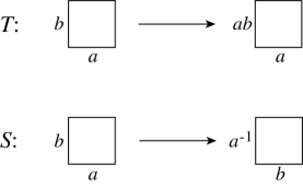
Figure 5.1: Modular transformations for a generic amplitude in orbifold models, where $a$, $b$ $\in\{{1,g,h,f}\}$ for a ${\mathbb{Z}}_{2}\times{\mathbb{Z}}_{2}$ orbifold.

which shows that the ${\mathbb{Z}}_{2}\times{\mathbb{Z}}_{2}$ orbifold needs at least two independent modular orbits. For example, the element $(g,h)$ cannot be derived from any untwisted amplitude. Therefore, to obtain the full partition function, we have to calculate each of the contributions shown in fig.5.2, where the empty and the coloured boxes are associated to two independent orbits. We remind that the full partition has to be modular invariant.

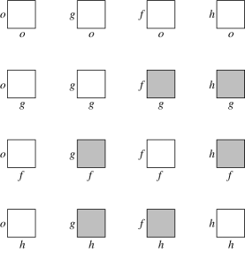
Figure 5.2: Modular orbits in ${\mathbb{Z}}_{2}\times{\mathbb{Z}}_{2}$ orbifolds.

At the end of this section we provide the result of the partition function in a compact form in the case without discrete torsion ($\epsilon=1$). In general, the value of the phase for the ${\mathbb{Z}}_{2}\times{\mathbb{Z}}_{2}$ case can be $\epsilon=\pm 1$ since it has to be of the same order as the generators of the orbifold. The explanations concerning the final form for the partition function (LABEL:z2xz2) are presented in the next sections and the definitions concerning the terms $T_{ij}$ and $G_{ij}$ are given in Appendix D.

The generic expression for a ${\mathbb{Z}}_{2}\times{\mathbb{Z}}_{2}$ orbifold partition function can be indicated as

$$\mathcal{Z}_{\text{Total}}=Tr_{(\text{un. + tw.})}\frac{1+g+f+h}{4}\,\,Z_{0},$$ (5.42)

where $Z_{0}$ in this case is given by eq.(LABEL:Z-). The explicit calculation of (5.42) gives

$$\mathcal{Z}_{\text{Total}}\!\!\! = \!\!{1\over 4}\biggl{\{}T_{oo}\Lambda_{1}\Lambda_{2}\Lambda_{m^{\prime},n^{\prime}}[\Lambda_{2m,n}(O_{16}O_{16}+C_{16}C_{16})+\Lambda_{2m+1,n}(S_{16}S_{16}+V_{16}V_{16})$$

$$+ \,\,\Lambda_{2m,n+\frac{1}{2}}(O_{16}C_{16}+C_{16}O_{16})+\Lambda_{2m+1,n+\frac{1}{2}}(V_{16}S_{16}+S_{16}V_{16})]$$

$$+ T_{og}\Lambda_{1}|{2\eta\over\theta_{2}}|^{4}G_{0g}+T_{of}\Lambda_{2}|{2\eta\over\theta_{2}}|^{4}G_{of}+T_{oh}\Lambda_{m^{\prime},n^{\prime}}|{2\eta\over\theta_{2}}|^{4}\big{\{}\Lambda_{2m,n}G_{oh}$$

$$+ \Lambda_{2m+1,n}G^{\prime}_{0h}+\Lambda_{2m,n+1/2}G^{\prime\prime}_{0h}+\Lambda_{2m+1,n+1/2}G^{\prime\prime\prime}_{0h}\big{\}}$$

$$+ T_{go}G_{g0}\Lambda_{1}|{2\eta\over\theta_{4}}|^{4}+T_{gg}G_{gg}\Lambda_{1}|{2\eta\over\theta_{3}}|^{4}+T_{fo}G_{fo}\Lambda_{2}|{2\eta\over\theta_{4}}|^{4}+T_{ff}G_{ff}\Lambda_{2}|{2\eta\over\theta_{3}}|^{4}$$

$$+ T_{ho}\Lambda_{mn}|{2\eta\over\theta_{4}}|^{4}\big{\{}\Lambda_{2mn}G_{h0}+\Lambda_{2m+1,n}G^{\prime}_{h0}+\Lambda_{2m,n+1/2}G^{\prime\prime}_{h0}+\Lambda_{2m+1,n+1/2}G^{\prime\prime\prime}_{h0}\big{\}}$$

$$+ T_{hh}\Lambda_{mn}|{2\eta\over\theta_{3}}|^{4}\big{\{}\Lambda_{2mn}G_{hh}+\Lambda_{2m+1,n}G^{\prime}_{hh}+\Lambda_{2m,n+1/2}G^{\prime\prime}_{hh}+\Lambda_{2m+1,n+1/2}G^{\prime\prime\prime}_{hh}\big{\}}$$

$$+ \left(T_{gh}G_{gh}+T_{gf}G_{gf}+T_{fg}G_{fg}+T_{fh}G_{fh}+T_{hg}G_{hg}+T_{hf}G_{hf}\right)|{8\eta^{3}\over{\theta_{2}\theta_{3}\theta_{4}}}|^{2}\biggr{\}}\quad,$$

where $\Lambda_{1}$, $\Lambda_{2}$ and $\Lambda_{m^{\prime}n^{\prime}}\Lambda_{mn}$ denote the three lattice sums associated to the three internal tori, as usual. The contributions of the transverse bosons is implicit here.

The details for the derivation of eq.(LABEL:z2xz2) are presented in the following sections, where we provide the main steps. In fact all the ingredients and the general methods have been presented extensively in the previous part of this chapter. The main difficulty for the ${\mathbb{Z}}_{2}\times{\mathbb{Z}}_{2}$ orbifold consists in handling correctly the numerous products of characters which have to be transformed under $S$ transformation. In fact they generate huge sums of terms which need some rearrangement to obtain a compact readable result. For this purpose a simple mathematica program has been used.

5.4.1 Untwisted spectrum

As in the calculation of eq.(5.7), the untwisted contribution is given by the sum of the projections w.r.t. the elements of the orbifold group of the initial partition function. The first four rows of eq.(LABEL:z2xz2) indicate the total untwisted sector.

The twisted sector is given by the sum of two pieces, the first is the S and T transformation of the untwisted contribution, the second is the new independent modular orbit with its S and T transforms. We provide some further information concerning the derivation of the twisted sector in the next section.

5.4.2 Twisted sector h

We present in the following the details for one twisted sector only, in particular the $h$ sector, where the element $G_{hg}$ fixes the choice of the independent orbit for our model by a consistent projection. In the other two twisted sectors there is no need for such a choice since all elements are determined by modular transformations from the previous ones. For the determination of a twisted sector $h$ we proceed, as usual, by taking the $S$ transform of the untwisted element projected by $h$. An $S$ transformation of $G_{0h}$ gives

$$G_{h0} = \big{\{}S_{2}C_{2}O_{2}O_{10}+C_{2}S_{2}V_{2}V_{10}+S_{2}S_{2}V_{2}O_{10}+C_{2}C_{2}O_{2}V_{10}$$ (5.44)

$$+C_{2}S_{2}O_{2}O_{10}+S_{2}C_{2}V_{2}V_{10}+C_{2}C_{2}V_{2}O_{10}+S_{2}S_{2}O_{2}V_{10}\big{\}}O_{16}$$

$$+\big{\{}V_{2}O_{2}S_{2}C_{10}+O_{2}V_{2}C_{2}S_{10}+O_{2}O_{2}S_{2}S_{10}+V_{2}V_{2}C_{2}C_{10}$$

$$+V_{2}O_{2}C_{2}S_{10}+O_{2}V_{2}S_{2}C_{10}+O_{2}O_{2}C_{2}C_{10}+V_{2}V_{2}S_{2}S_{10}\big{\}}C_{16}.$$

The T transformation of (5.44) provides the contribution $G_{hh}$ and in its expression we include the total phase arising from the following overall phases

$$G_{h0}\quad\underrightarrow{T}\quad iG_{hh}\quad,\quad T_{h0}\quad\underrightarrow{T}\quad iT_{hh}\quad\Rightarrow i\times i\times-1=+1,$$

where the last $-1$ in the formula is the global prefactor obtained in the T transformations (see eq.(5.27)).

$$G_{hh} = \big{\{}S_{2}C_{2}O_{2}O_{10}+C_{2}S_{2}V_{2}V_{10}-S_{2}S_{2}V_{2}O_{10}-C_{2}C_{2}O_{2}V_{10}$$ (5.45)

$$+C_{2}S_{2}O_{2}O_{10}+S_{2}C_{2}V_{2}V_{10}-C_{2}C_{2}V_{2}O_{10}-S_{2}S_{2}O_{2}V_{10}\big{\}}O_{16}$$

$$+\big{\{}V_{2}O_{2}S_{2}C_{10}+O_{2}V_{2}C_{2}S_{10}-O_{2}O_{2}S_{2}S_{10}-V_{2}V_{2}C_{2}C_{10}$$

$$+V_{2}O_{2}C_{2}S_{10}+O_{2}V_{2}S_{2}C_{10}-O_{2}O_{2}C_{2}C_{10}-V_{2}V_{2}S_{2}S_{10}\big{\}}C_{16}.$$

The independent orbit $G_{hg}$ is obtained by the action of the $g$ element onto $G_{h0}$. The overall phase is included in the final expression (5.46) and results from

$$G_{h0}\quad\underrightarrow{g}\quad iG_{hg}\quad,\quad T_{h0}\quad\underrightarrow{g}\quad iT_{hg}\quad\Rightarrow i\times i=-1.$$

$$G_{hg} = \big{\{}S_{2}C_{2}O_{2}O_{10}+C_{2}S_{2}V_{2}V_{10}+S_{2}S_{2}V_{2}O_{10}+C_{2}C_{2}O_{2}V_{10}$$ (5.46)

$$-C_{2}S_{2}O_{2}O_{10}-S_{2}C_{2}V_{2}V_{10}-C_{2}C_{2}V_{2}O_{10}-S_{2}S_{2}O_{2}V_{10}\big{\}}O_{16}$$

$$+(-1)\big{\{}-V_{2}O_{2}S_{2}C_{10}-O_{2}V_{2}C_{2}S_{10}-O_{2}O_{2}S_{2}S_{10}-V_{2}V_{2}C_{2}C_{10}$$

$$+V_{2}O_{2}C_{2}S_{10}+O_{2}V_{2}S_{2}C_{10}+O_{2}O_{2}C_{2}C_{10}+V_{2}V_{2}S_{2}S_{10}\big{\}}C_{16}.$$

We observe that the choice for our projection is not the conventional one since after performing the $g$ action onto the gauge degrees of freedom we also added a minus sign in front of all the terms multiplying $C_{16}$. This operation provides a natural result for $G_{hg}$, meaning that the composition of the characters is analogous to $G_{h0}$ and $G_{hh}$ and assures the modular invariance of the partition function.

The T transformation of eq.(5.46) provides $G_{hf}$ which, as usual, includes the total phase from

$$G_{hg}\quad\underrightarrow{T}\quad iG_{hf}\quad,\quad T_{hg}\quad\underrightarrow{T}\quad iT_{hf}\quad\Rightarrow i\times i\times-1=+1.$$

$$G_{hf} = \big{\{}S_{2}C_{2}O_{2}O_{10}+C_{2}S_{2}V_{2}V_{10}-S_{2}S_{2}V_{2}O_{10}-C_{2}C_{2}O_{2}V_{10}$$ (5.47)

$$-C_{2}S_{2}O_{2}O_{10}-S_{2}C_{2}V_{2}V_{10}+C_{2}C_{2}V_{2}O_{10}+S_{2}S_{2}O_{2}V_{10}\big{\}}O_{16}$$

$$+\big{\{}V_{2}O_{2}S_{2}C_{10}+O_{2}V_{2}C_{2}S_{10}-O_{2}O_{2}S_{2}S_{10}-V_{2}V_{2}C_{2}C_{10}$$

$$-V_{2}O_{2}C_{2}S_{10}-O_{2}V_{2}S_{2}C_{10}+O_{2}O_{2}C_{2}C_{10}+V_{2}V_{2}S_{2}S_{10}\big{\}}C_{16}.$$

We have an important comment to make before discussing the relevant parts of the spectrum. In the untwisted sector generated by the $h$ element there are gauge contributions ($G^{\prime}_{0h}$, $G^{\prime\prime}_{0h}$, $G^{\prime\prime\prime}_{0h}$) which are multiplied by massive lattices, not providing any low energy states. In the $h$ twisted part these terms can still give a contribution to the massless spectrum (since we rearrange the lattices with the transformations (LABEL:prop). The presence of the terms $G^{\prime}_{h0}$, $G^{\prime\prime}_{h0}$, $G^{\prime\prime\prime}_{h0}$ and their T transformations will not provide massless states. Thus, we can neglect these contributions when we discuss the relevant part of the spectrum.

5.4.3 Torus amplitudes for the right and for the left sector

In the result (LABEL:z2xz2) we have used the torus amplitudes defined in terms of the quantities $T_{ij}$, $i=0,g,h,f$, providing a simple and compact form for the partition function.

$$T_{i0} = \tau_{i0}+\tau_{ig}+\tau_{ih}+\tau_{if}\quad,\qquad T_{ig}=\tau_{i0}+\tau_{ig}-\tau_{ih}-\tau_{if}\quad,$$

$$T_{ih} = \tau_{i0}-\tau_{ig}+\tau_{ih}-\tau_{if}\quad,\qquad T_{if}=\tau_{i0}-\tau_{ig}-\tau_{ih}+\tau_{if}\quad,$$ (5.48)

where the ${\mathbb{Z}}_{2}\times{\mathbb{Z}}_{2}$ characters $\tau_{ij}$ are products of the four level-one characters, defined explicitly in (D.3). The ordering of the four factors refers to the eight transverse dimensions of spacetime. The first factor is associated to the two transverse space time directions. For the left sector we have

$$G_{i0} = g_{i0}+g_{ig}+g_{ih}+g_{if}\quad,\qquad G_{ig}=g_{i0}+g_{ig}-g_{ih}-g_{if}\quad,$$

$$G_{ih} = g_{i0}-g_{ig}+g_{ih}-g_{if}\quad,\qquad G_{if}=g_{i0}-g_{ig}-g_{ih}+g_{if}\quad.$$ (5.49)

The content of the above definitions is given in (D.2). There we also provide the explicit expressions for the gauge contributions $G^{\prime}_{0h}$, $G^{\prime\prime}_{0h}$, $G^{\prime\prime\prime}_{0h}$ for the untwisted sector and $G^{\prime}_{h0}$, $G^{\prime\prime}_{h0}$ and $G^{\prime\prime\prime}_{h0}$ for the twisted sector.

5.4.4 Massless spectrum

The formula (LABEL:z2xz2) presents the full modular invariant partition function for the shift orbifold (LABEL:Z-) with ${\mathbb{Z}}_{2}\times{\mathbb{Z}}_{2}$ action. We notice that the only contributions from the untwisted spectrum, where we have neglected the accented expressions, come from the combinations

$$\tau_{00}g_{00}+\tau_{0g}g_{0g}+\tau_{0h}g_{0h}+\tau_{0f}g_{0f}.$$ (5.50)

Our main interest is as usual the low energy physics of the model hence we will present here the massless terms, which can be expanded in powers of $q$ by applying the relations of section A.3 in Appendix A.

$$[\overline{V}_{2}\overline{O}_{2}\overline{O}_{2}\overline{O}_{2}-\overline{S}_{2}\overline{S}_{2}\overline{S}_{2}\overline{S}_{2}-\overline{C}_{2}\overline{C}_{2}\overline{C}_{2}\overline{C}_{2}]\times[O_{2}O_{2}O_{2}O_{10}O_{16}],$$

$$[\overline{O}_{2}\overline{V}_{2}\overline{O}_{2}\overline{O}_{2}-\overline{C}_{2}\overline{C}_{2}\overline{S}_{2}\overline{S}_{2}-\overline{S}_{2}\overline{S}_{2}\overline{C}_{2}\overline{C}_{2}]\times[(O_{2}V_{2}V_{2}O_{10}+V_{2}O_{2}O_{2}V_{10})O_{16}],$$

$$[\overline{O}_{2}\overline{O}_{2}\overline{O}_{2}\overline{V}_{2}-\overline{C}_{2}\overline{S}_{2}\overline{S}_{2}\overline{C}_{2}-\overline{S}_{2}\overline{C}_{2}\overline{C}_{2}\overline{S}_{2}]\times[(V_{2}V_{2}O_{2}O_{10}+O_{2}O_{2}V_{2}V_{10})O_{16}],$$

$$[\overline{O}_{2}\overline{O}_{2}\overline{V}_{2}\overline{O}_{2}-\overline{C}_{2}\overline{S}_{2}\overline{C}_{2}\overline{S}_{2}-\overline{S}_{2}\overline{C}_{2}\overline{S}_{2}\overline{C}_{2}]\times[(V_{2}O_{2}V_{2}O_{10}+O_{2}V_{2}O_{2}V_{10})O_{16}].$$

(5.51)

The gauge group of this model is given by $G=SO(2)\times SO(2)\times SO(2)\times SO(10)\times SO(16)$ and the representations of the untwisted matter is provided in the following.

$\bullet$ Vectorial supermultiplet:

$$[\overline{V}_{2}\overline{O}_{2}\overline{O}_{2}\overline{O}_{2}-\overline{S}_{2}\overline{S}_{2}\overline{S}_{2}\overline{S}_{2}-\overline{C}_{2}\overline{C}_{2}\overline{C}_{2}\overline{C}_{2}]\times[O_{2}O_{2}O_{2}O_{10}O_{16}]\rightarrow$$

$$[(2,1,1,1)+(1^{+},1^{+},1^{+},1^{+})+(1^{-},1^{-},1^{-},1^{-})]\times(1,1,1,1,1)$$

$\bullet$ Two chiral supermultiplets:

$$[\overline{O}_{2}\overline{V}_{2}\overline{O}_{2}\overline{O}_{2}-\overline{C}_{2}\overline{C}_{2}\overline{S}_{2}\overline{S}_{2}-\overline{S}_{2}\overline{S}_{2}\overline{C}_{2}\overline{C}_{2}]\times[(O_{2}V_{2}V_{2}O_{10}+V_{2}O_{2}O_{2}V_{10})O_{16}]\rightarrow$$

$$[(1,2,1,1)+(1^{-},1^{-},1^{+},1^{+})+(1^{+},1^{+},1^{-},1^{-})]\times[(1,2,2,1,1)+(2,1,1,10,1)]$$

$\bullet$ Two chiral supermultiplets:

$$[\overline{O}_{2}\overline{O}_{2}\overline{O}_{2}\overline{V}_{2}-\overline{C}_{2}\overline{S}_{2}\overline{S}_{2}\overline{C}_{2}-\overline{S}_{2}\overline{C}_{2}\overline{C}_{2}\overline{S}_{2}]\times[(V_{2}V_{2}O_{2}O_{10}+O_{2}O_{2}V_{2}V_{10})O_{16}]\rightarrow$$

$$[(1,1,1,2)+(1^{-}1^{+}1^{+}1^{-})+(1^{+}1^{-}1^{-}1^{+})]\times[(2,2,1,1,1)+(1,1,2,10,1)]$$

$\bullet$ Two chiral supermultiplets:

$$[\overline{O}_{2}\overline{O}_{2}\overline{V}_{2}\overline{O}_{2}-\overline{C}_{2}\overline{S}_{2}\overline{C}_{2}\overline{S}_{2}-\overline{S}_{2}\overline{C}_{2}\overline{S}_{2}\overline{C}_{2}]\times[(V_{2}O_{2}V_{2}O_{10}+O_{2}V_{2}O_{2}V_{10})O_{16}]\rightarrow$$

$$[(1,1,2,1)+(1^{-}1^{+}1^{-}1^{+})(1^{+}1^{-}1^{+}1^{-})]\times[(2,1,2,1,1)+(1,2,1,10,1)].$$

In our notations we indicate with $1^{\pm}$ the two different chiralities of a spinor in the $SO(2)$ representation. This model has $N=1$ in four dimensions.

The twisted sector gives rise to the only non-vanishing terms

$$\tau_{g0}g_{g0}+\tau_{gg}g_{gg}+\tau_{gh}g_{gh}+\tau_{gf}g_{gf}+\tau_{h0}g_{h0}+\tau_{hg}g_{hg}$$

$$+\tau_{hh}g_{hh}+\tau_{hf}g_{hf}+\tau_{f0}g_{f0}+\tau_{fg}g_{fg}+\tau_{fh}g_{fh}+\tau_{ff}g_{ff},$$ (5.52)

whose massless contributions have been indicated in the following

$$[\overline{O}_{2}\overline{O}_{2}\overline{C}_{2}\overline{C}_{2}-\overline{C}_{2}\overline{S}_{2}\overline{O}_{2}\overline{O}_{2}]\times[(C_{2}O_{2}O_{2}C_{10}+V_{2}C_{2}C_{2}O_{10}+O_{2}S_{2}S_{2}V_{10})O_{16}],$$

$$[\overline{O}_{2}\overline{O}_{2}\overline{S}_{2}\overline{S}_{2}-\overline{S}_{2}\overline{C}_{2}\overline{O}_{2}\overline{O}_{2}]\times[(S_{2}O_{2}O_{2}S_{10}+V_{2}S_{2}S_{2}O_{10}+O_{2}C_{2}C_{2}V_{10})O_{16}],$$

$$[\overline{O}_{2}\overline{C}_{2}\overline{C}_{2}\overline{O}_{2}-\overline{C}_{2}\overline{O}_{2}\overline{O}_{2}\overline{S}_{2}]\times[(C_{2}C_{2}V_{2}O_{10}+S_{2}S_{2}O_{2}V_{10})O_{16}],$$

$$[\overline{O}_{2}\overline{S}_{2}\overline{S}_{2}\overline{O}_{2}-\overline{S}_{2}\overline{O}_{2}\overline{O}_{2}\overline{C}_{2}]\times[(S_{2}S_{2}V_{2}O_{10}+C_{2}C_{2}O_{2}V_{10})O_{16}],$$

$$[\overline{O}_{2}\overline{S}_{2}\overline{O}_{2}\overline{S}_{2}-\overline{S}_{2}\overline{O}_{2}\overline{C}_{2}\overline{O}_{2}]\times[(O_{2}S_{2}O_{2}S_{10}+S_{2}V_{2}S_{2}O_{10}+C_{2}O_{2}C_{2}V_{10})O_{16}],$$

$$[\overline{O}_{2}\overline{C}_{2}\overline{O}_{2}\overline{C}_{2}-\overline{C}_{2}\overline{O}_{2}\overline{S}_{2}\overline{O}_{2}]\times[(O_{2}C_{2}O_{2}C_{10}+C_{2}V_{2}C_{2}O_{10}+S_{2}O_{2}S_{2}V_{10})O_{16}].$$

(5.53)

These chiral supermultiplets fall into the representations presented below.

$\bullet$ Three chiral supermultiplets:

$$[\overline{O}_{2}\overline{O}_{2}\overline{C}_{2}\overline{C}_{2}-\overline{C}_{2}\overline{S}_{2}\overline{O}_{2}\overline{O}_{2}]\times[(C_{2}O_{2}O_{2}C_{10}+V_{2}C_{2}C_{2}O_{10}+O_{2}S_{2}S_{2}V_{10})O_{16}]+$$

$$\,\,[\overline{O}_{2}\overline{O}_{2}\overline{S}_{2}\overline{S}_{2}-\overline{S}_{2}\overline{C}_{2}\overline{O}_{2}\overline{O}_{2}]\times[(S_{2}O_{2}O_{2}S_{10}+V_{2}S_{2}S_{2}O_{10}+O_{2}C_{2}C_{2}V_{10})O_{16}]\rightarrow$$

$$[(1,1,1^{\pm},1^{\pm})+(1^{\pm},1^{\pm},1,1)]\times[(1^{\pm},1,1,16,1)+(2,1^{\pm},1^{\pm},1,1)+(1,1^{\pm},1^{\pm},10,1)]$$

$\bullet$ Two chiral supermultiplets:

$$[\overline{O}_{2}\overline{C}_{2}\overline{C}_{2}\overline{O}_{2}-\overline{C}_{2}\overline{O}_{2}\overline{O}_{2}\overline{S}_{2}]\times[(C_{2}C_{2}V_{2}O_{10}+S_{2}S_{2}O_{2}V_{10})O_{16}]+$$

$$\,\,\,[\overline{O}_{2}\overline{S}_{2}\overline{S}_{2}\overline{O}_{2}-\overline{S}_{2}\overline{O}_{2}\overline{O}_{2}\overline{C}_{2}]\times[(S_{2}S_{2}V_{2}O_{10}+C_{2}C_{2}O_{2}V_{10})O_{16}]\rightarrow$$

$$[(1,1^{\pm},1^{\pm},1)+(1^{\pm},1,1,1^{\pm})]\times[(1^{\pm},1^{\pm},2,1,1)+(1^{\pm},1^{\pm},1,10,1)]$$

$\bullet$ Three chiral supermultiplets:

$$[\overline{O}_{2}\overline{S}_{2}\overline{O}_{2}\overline{S}_{2}-\overline{S}_{2}\overline{O}_{2}\overline{C}_{2}\overline{O}_{2}]\times[(O_{2}S_{2}O_{2}S_{10}+S_{2}V_{2}S_{2}O_{10}+C_{2}O_{2}C_{2}V_{10})O_{16}]+$$

$$\,\,[\overline{O}_{2}\overline{C}_{2}\overline{O}_{2}\overline{C}_{2}-\overline{C}_{2}\overline{O}_{2}\overline{S}_{2}\overline{O}_{2}]\times[(O_{2}C_{2}O_{2}C_{10}+C_{2}V_{2}C_{2}O_{10}+S_{2}O_{2}S_{2}V_{10})O_{16}]\rightarrow$$

$$[(1,1^{\pm},1,1^{\pm})+(1^{\pm},1,1^{\pm},1)]\times[(1,1^{\pm},1,16,1)+(1^{\pm},2,1^{\pm},1,1)+(1^{\pm},1,1^{\pm},10,1)].$$

We notice that the twisted massless spectrum contains two chiral supermultiplets in the spinorial representation of $SO(10)$, plus few supermultiplets in the fundamental of $SO(10)$ in four dimensions. This result concludes our chapter.

Chapter 6 Conclusions

In this thesis we focus our study on heterotic superstring theories and their applications to particle physics. In particular, we are interested in the search of semi-realistic four-dimensional superstring vacua which can reproduce, at low energy, the Standard Model physics. Motivated by the $SO(10)$ embedding of matter in heterotic models, we investigate different schemes of compactification of the $E_{8}\times E_{8}$ heterotic string from ten to four dimensions. A very successful approach is given by free fermionic models. They give rise to the most realistic three generation string models to date. Their phenomenology is studied in the effective low energy field theory by the analysis of supersymmetric flat directions. In the first example illustrated in chapter 3, the model content consists of MSSM states in the observable Standard Model sector. In that model, for the first time, we apply a new general mechanism that allows the reduction of Higgs content at the string scale by an opportune choice of asymmetric boundary conditions for the internal fermions of the theory. An additional result for minimal Higgs spectrum models is the fact that the supersymmetric moduli space is reduced as well, and this increases the predictive power of the theory.

A common feature of free fermionic models is the presence of an anomalous $U(1)$ which gives rise to a Fayet-Iliopoulos D-term that breaks supersymmetry at one-loop level in string perturbation theory. Supersymmetry is restored by imposing D and F flatness on the vacuum. Generally, it has been assumed that in a given string model there should exist a supersymmetric solution to D and F flatness constraints. Nevertheless, in the second model presented in chapter 3, such as in the previous example, no flat solutions are found after employing the standard analysis for flat directions. The Bose-Fermi degeneracy of the spectrum implies that the cosmological constant vanishes while supersymmetry remains broken at the perturbative level. This unexpected result may open new possibilities for the supersymmetry breaking mechanism in string theory. By looking at a very different background, the one given by the orbifold construction, it is possible to obtain complementary advantages in the understanding of semi-realistic models, such as a more geometric picture of those. Moreover, in the case of ${\mathbb{Z}}_{2}\times{\mathbb{Z}}_{2}$ for special points in the compactification space, the correspondence with free fermionic models has been demonstrated. This connection offers interesting indications in the choice of "good" orbifolds, since the number of consistent models is huge and a guiding principle is needed. A specific ${\mathbb{Z}}_{2}\times{\mathbb{Z}}_{2}$ orbifold with a non-factorisable skewed compactification lattice has been analysed, where the reduction of the number of families is realised and suggests new way of investigating orbifold compactifications. No semi-realistic models are presented in this set up yet, nevertheless the possible combinations of a proper choice for the compactification lattice plus the presence of suitable Wilson lines provides new chances in the construction of semi-realistic models. A challenging outlook in this set up is the introduction of asymmetric shifts and twists. Indeed, these elements seem to be related with free fermionic models where asymmetric boundary conditions are imposed on the compact dimensions and are responsible for the most successful phenomenological features of these models.

In the last chapter we present the formalism for the construction of modular invariant partition functions in heterotic orbifold models and, among a few examples, the case of a ${\mathbb{Z}}_{2}\times{\mathbb{Z}}_{2}$ shift orbifold model. The study of orbifolds with different projections should lighten the properties of the low energy spectrum and possibly provide some selection mechanism for semi-realistic vacua. For instance, a challenging project would be the realisation of the Higgs-matter splitting. This mechanism is viable with an orbifold projection that will allow to obtain string states uniquely from the untwisted sector and the matter states from the twisted sectors. This mechanism is already well-known in the free fermionic case.

Appendix A

A.1 $\eta$ and $\theta$-functions and modular transformations

The Dedekind $\eta$ function is defined as

$$\eta(\tau)=q^{\frac{1}{24}}\prod_{p=1}^{\infty}(1-q^{p}).$$ (A.1)

We provide the modular transformations of $\eta$ and of the Teichmuller parameter $\tau$ in terms of complex function and real components.

$$T:\eta(1+\tau)=e^{i\pi/12}\eta(\tau)\quad,\quad S:\eta(-\frac{1}{\tau})=(-i\tau)^{\frac{1}{2}}\eta(\tau).$$ (A.2)

$$T:\tau_{1}\rightarrow\tau_{1}+1\quad;\quad\tau_{2}\rightarrow\tau_{2}\quad;\quad d\tau_{1}d\tau_{2}\rightarrow d\tau_{1}d\tau_{2}.$$

$$S:\tau_{1}+i\tau_{2}\rightarrow-\frac{1}{\tau_{1}+i\tau_{2}}=-\frac{\bar{\tau}}{\tau\bar{\tau}}\quad;\quad d\tau d\bar{\tau}\rightarrow\frac{d\tau d\bar{\tau}}{|\tau\bar{\tau}|^{2}}.$$

The definition of the $\theta$ function is given in both notations, as sum and as product formulae

$$\theta\left[\begin{array}[]{c}\alpha\\ \beta\end{array}\right](0|\theta) = \sum_{n=\infty}^{\infty}q^{\frac{1}{2}(n+\alpha)^{2}}e^{2\pi i(n+\alpha)\beta}$$

$$= e^{2\pi i\alpha\beta}q^{\frac{\alpha^{2}}{2}}\prod_{n}^{\infty}(1-q^{n})(1+q^{n+\alpha-\frac{1}{2}}e^{2\pi i\beta})(1+q^{n-\alpha-\frac{1}{2}}e^{-2\pi i\beta})$$

and their modular transformations

$$T:\theta\left[\begin{array}[]{c}\alpha\\ \beta\end{array}\right](0|\tau+1)=e^{-\pi i\alpha(\alpha-1)}\,\,\,\theta\left[\begin{array}[]{c}\alpha\\ \beta+\alpha-\frac{1}{2}\end{array}\right](0|\tau),$$ (A.11)

$$S:\theta\left[\begin{array}[]{c}\alpha\\ \beta\end{array}\right](0|-\frac{1}{\tau})=\,\,\,(-i\tau)^{\frac{1}{2}}\,\,\,e^{2\pi i\alpha\beta}\,\,\,\theta\left[\begin{array}[]{c}\beta\\ -\alpha\end{array}\right](0|\tau).$$ (A.16)

A.1.1 $SO(2n)$ characters in terms of $\theta$-functions

$$O_{2n}=\frac{\theta^{n}_{3}+\theta^{n}_{4}}{2\eta^{n}}\,\,\,\,;\,\,\,\,V_{2n}=\frac{\theta^{n}_{3}-\theta^{n}_{4}}{2\eta^{n}}\,\,\,\,;\,\,\,\,S_{2n}=\frac{\theta^{n}_{2}+i^{-n}\theta^{n}_{1}}{2\eta^{n}}\,\,\,\,;\,\,\,\,C_{2n}=\frac{\theta^{n}_{2}-i^{-n}\theta^{n}_{1}}{2\eta^{n}}\,\,\,\,.\,\,\,\,$$ (A.17)

It is useful to present the explicit expansions of the previous functions and the $\eta$ function in terms of powers of $q$, where $q=e^{2i\pi\tau}$

$$O_{2n}= \frac{\Pi_{p=1}^{\infty}(1-q^{p})^{n}(1+q^{p-\frac{1}{2}})^{2n}+\Pi_{p=1}^{\infty}(1-q^{p})^{n}(1-q^{p-\frac{1}{2}})^{2n}}{2q^{\frac{n}{24}}\Pi_{p=1}^{\infty}(1-q^{p})^{n}}$$

$$= q^{-\frac{n}{24}}(1+n(2n-1)q+...),$$

$$V_{2n}= \frac{\Pi_{p=1}^{\infty}(1-q^{p})^{n}(1+q^{p-\frac{1}{2}})^{2n}-\Pi_{p=1}^{\infty}(1-q^{p})^{n}(1-q^{p-\frac{1}{2}})^{2n}}{2q^{\frac{n}{24}}\Pi_{p=1}^{\infty}(1-q^{p})^{n}}$$

$$= q^{-\frac{n}{24}}(2nq^{\frac{1}{2}}+...),$$

$$S_{2n}/C_{2n}= q^{\frac{n}{8}}\frac{\Pi_{p=1}^{\infty}(1-q^{p})^{n}(1+q^{p})^{n}(1+q^{p-1})^{n}}{2q^{\frac{n}{24}}\Pi_{p=1}^{\infty}(1-q^{p})^{n}}$$

$$= 2^{n-1}q^{\frac{n}{12}}(1+2nq+...),$$

$$\frac{1}{\eta^{n}}= q^{-\frac{n}{24}}(1+nq+...),$$ (A.18)

where the definition of $\theta$-functions and the binomial expansion below have been applied,

$$(a+b)^{n}=\sum_{i=0}^{n}C\left(\begin{array}[]{c}n\\ i\\ \end{array}\right)a^{n-i}b^{i}=a^{n}+C\left(\begin{array}[]{c}n\\ i\\ \end{array}\right)a^{n-1}b+...\,.$$

The decomposition of an $SO(x+y)$ character into the product of an $SO(x)$ with an $SO(y)$ character is given by the expressions below:

$$O_{2n} = O_{x}O_{y}+V_{x}V_{y},\hskip 28.45274ptV_{2n}=V_{x}O_{y}+O_{x}V_{y},$$

$$C_{2n} = S_{x}C_{y}+C_{x}S_{y},\hskip 28.45274ptS_{2n}=S_{x}S_{y}+C_{x}C_{y},$$ (A.19)

where $2n=x+y$ and $x,y$ are even.

In the study of the S transformations of the previous expansions it can be useful to rearrange (A.19) with the relations

$$aa+bb = \frac{1}{2}[(a+b)(a+b)+(a-b)(a-b)]$$

$$aa-bb = \frac{1}{2}[(a-b)(a+b)+(a+b)(a-b)]$$

$$ab+ba = \frac{1}{2}[(a+b)(a+b)-(a-b)(a-b)]$$

$$ab-ba = \frac{1}{2}[(a-b)(a+b)-(a+b)(a-b)]$$ (A.20)

where $a$ and $b$ can be any of $O_{n},V_{n},S_{n},C_{n}$.

A.1.2 Modular transformations for $SO(2n)$ characters

The modular S and T transformations act on the characters as

$$\left(\begin{array}[]{c}O_{2n}\\ V_{2n}\\ S_{2n}\\ C_{2n}\\ \end{array}\right)\,\,\,\,\,\,\,\,\underrightarrow{S}\,\,\,\,\,\,\,\frac{1}{2}\left(\begin{array}[]{cccc}1&1&1&1\\ 1&1&-1&-1\\ 1&-1&i^{-n}&-i^{-n}\\ 1&-1&-i^{-n}&i^{-n}\\ \end{array}\right)\left(\begin{array}[]{c}O_{2n}\\ V_{2n}\\ S_{2n}\\ C_{2n}\\ \end{array}\right);$$ (A.33)

$$\left(\begin{array}[]{c}O_{2n}\\ V_{2n}\\ S_{2n}\\ C_{2n}\\ \end{array}\right)\,\,\,\,\,\,\,\,\,\underrightarrow{T}\,\,e^{-in\pi/12}\,\,\left(\begin{array}[]{cccc}1&0&0&0\\ 0&-1&0&0\\ 0&0&e^{in\pi/4}&0\\ 0&0&0&e^{in\pi/4}\\ \end{array}\right)\left(\begin{array}[]{c}O_{2n}\\ V_{2n}\\ S_{2n}\\ C_{2n}\\ \end{array}\right).$$ (A.46)

(A.47)

A.2 Definition of lattice

The partition function of a compact scalar on a circle of radius $R$ is

$$\Lambda_{m,n}=\frac{1}{\eta\overline{\eta}}\sum_{m,n}q^{\alpha^{\prime}p_{L}^{2}/4}\overline{q}^{\alpha^{\prime}p_{R}^{2}/4},$$ (A.48)

where the chiral momenta are defined as

$$p_{L,R}=\frac{m}{R}\pm\frac{nR}{\alpha^{\prime}}.$$

Therefore, if one of the non-compact coordinates of a critical string is replaced with a compact one, the continuous integration over internal momenta is replaced by the lattice sum $\frac{1}{\sqrt{\tau_{2}}\eta(\tau)\overline{\eta}(\tau)}\rightarrow\Lambda_{m,n}$.

For the case of a d-dimensional torus the eq.(A.48) is generalised to

$$\vec{\Lambda}_{m,n}=\frac{1}{\eta^{d}\overline{\eta}^{d}}\sum_{m,n}q^{\alpha^{\prime}p_{L}^{T}g^{-1}p_{L}/4}\overline{q}^{\alpha^{\prime}p_{R}^{T}g^{-1}p_{R}/4}$$ (A.49)

where $p_{L,a}={m_{a}}+\frac{1}{\alpha^{\prime}}(g_{ab}-B_{ab})n^{b}$, $p_{R,a}={m_{a}}+\frac{1}{\alpha^{\prime}}(g_{ab}+B_{ab})n^{b}$, $g_{ab}$ is the metric on the torus and $B_{ab}$ is an antisymmetric NS-NS field.

A.2.1 Definition of shifted lattices

In this section we present combinations obtained with the standard lattice $\Lambda_{mn}$ when the shift $\delta:\Lambda_{m,n}\rightarrow(-1)^{m}\Lambda_{m,n}$ acts on it. Moreover we show their main properties whose demonstration is given in section A.2.2.

$$\Lambda_{2m,n} = \frac{1+(-1)^{m}}{2}\Lambda_{m,n},$$

$$\Lambda_{2m+1,n} = \frac{1-(-1)^{m}}{2}\Lambda_{m,n},$$

$$\Lambda_{2m,n+\frac{1}{2}} = \frac{1+(-1)^{m}}{2}\Lambda_{m,n+\frac{1}{2}},$$

$$\Lambda_{2m+1,n+\frac{1}{2}} = \frac{1-(-1)^{m}}{2}\Lambda_{m,n+\frac{1}{2}}.$$

Transformation properties

$$\overbrace{\Lambda_{m,n}}^{\mathit{S\,,\,T\,\,invariant}}\,\,\,;\,\,\,\overbrace{\Lambda_{2m,n}+\Lambda_{2m,n+\frac{1}{2}}}^{\mathit{S\,,\,T\,\,invariant}}$$

$$\overbrace{(-1)^{m}\Lambda_{m,n}}^{\mathit{T\,\,invariant}}\,\,\,\,\underrightarrow{\mathit{{S}}}\,\,\,\,\Lambda_{m,n+\frac{1}{2}}\,\,\,\,\underrightarrow{\mathit{T}}\,\,\,\,\overbrace{(-1)^{m}\Lambda_{m,n+\frac{1}{2}}}^{\mathit{S\,\,invariant}}$$

$$\overbrace{\Lambda_{2m,n}-\Lambda_{2m,n+\frac{1}{2}}}^{\mathit{T\,\,invariant}}\,\,\,\,\underrightarrow{\mathit{{S}}}\,\,\,\,\Lambda_{2m+1,n}+\Lambda_{2m+1,n+\frac{1}{2}}\,\,\,\,\underrightarrow{\mathit{T}}\,\,\,\,\overbrace{\Lambda_{2m+1,n}-\Lambda_{2m+1,n+\frac{1}{2}}}^{\mathit{S\,\,invariant}}$$ .

A.2.2 Proof for the transformation properties (LABEL:prop)

In this section we show how to derive some of the properties presented in the previous section.

• $S$ invariance for $\Lambda_{m,n}$.

• $T$ invariance for $\Lambda_{m,n}$ and $(-1)^{m}\Lambda_{m,n}$.

• $(-1)^{m}\Lambda_{m,n}\quad\underrightarrow{S}\quad\Lambda_{m,n+1/2}$.

The other relations shown in (LABEL:prop) can be derived with the same techniques below.

It is useful to keep in mind the definitions of the general lattice (A.48) and the chiral momenta $p_{L,R}$. Moreover we can rewrite $q$ and $\bar{q}$ in the convenient way

$$q=e^{2\pi i\tau}=e^{2\pi i(\tau_{1}+i\tau_{2})}=e^{2\pi(i\tau_{1}-\tau_{2})},\quad\bar{q}=e^{-2\pi i\bar{\tau}}=e^{-2\pi i(\tau_{1}-i\tau_{2})}=e^{-2\pi(i\tau_{1}+\tau_{2})}.$$

The Poisson resummation formula will be applied constantly in the demonstration of the previous statements, thus we provide its general expression below

$$\sum_{m_{i}\in Z}e^{-\pi m_{i}\cdot m_{j}A_{ij}+\pi B_{i}m_{i}}=\frac{1}{\sqrt{\text{det}A}}\sum_{m_{k}\in Z}e^{-\pi(m_{k}+\frac{iB_{k}}{2})(A^{-1})_{kl}(m_{l}+\frac{iB_{l}}{2})}$$ (A.52)

We start by demonstrating point 1).

The best way to proceed is to rewrite the lattice sum in the more convenient form

$$\Lambda_{m,n}=\sum_{m,n}e^{2\pi(i\tau_{1}-\tau_{2})\frac{\alpha^{\prime}}{4}(\frac{m}{R}+\frac{nR}{\alpha^{\prime}})^{2}}e^{2\pi(-i\tau_{1}-\tau_{2})\frac{\alpha^{\prime}}{4}(\frac{m}{R}-\frac{nR}{\alpha^{\prime}})^{2}}.$$ (A.53)

We notice that the $\frac{1}{\eta\bar{\eta}}$ factor has been dropped for convenience.

Let us simplify the two exponentials and rewrite

$$\Lambda_{m,n}=\sum_{m,n}e^{2\pi i\tau_{1}mn}e^{-\pi\tau_{2}\alpha^{\prime}(\frac{m^{2}}{R^{2}}+\frac{n^{2}R^{2}}{\alpha^{\prime 2}})}.$$ (A.54)

If we perform a Poisson resummation w.r.t. $m$ we have

$$a=\frac{\alpha^{\prime}\tau_{2}}{R^{2}}\rightarrow\frac{1}{\sqrt{detA}}=\frac{R}{\sqrt{\alpha^{\prime}\tau_{2}}},\quad b=2i\pi n$$

then eq.(A.54) becomes

$$\frac{R}{\sqrt{\alpha^{\prime}\tau_{2}}}\sum_{m,n}e^{-\pi(m^{\prime}-\tau_{1}n)^{2}\frac{R^{2}}{\alpha^{\prime}\tau_{2}}}e^{-\pi\tau_{2}\frac{n^{2}R^{2}}{\alpha^{\prime}}}.$$ (A.55)

We expand the square and we obtain an exponential with four terms. Two of them can be rewritten as

$$-\frac{\pi R^{2}}{\alpha^{\prime}}(\frac{\tau_{1}^{2}}{\tau_{2}}+\tau_{2})n^{2}=-\frac{\pi R^{2}}{\alpha^{\prime}}\frac{|\tau|^{2}}{\tau_{2}}n^{2}.$$

We apply now the resummation w.r.t. $n$

$$a=\frac{R^{2}|\tau^{2}|}{\alpha^{\prime}\tau_{2}}\rightarrow\frac{1}{\sqrt{detA}}=\frac{\sqrt{\alpha^{\prime}\tau_{2}}}{R|\tau|},\quad b=\frac{2R^{2}\tau_{1}m^{\prime}}{\tau_{2}\alpha^{\prime}}$$

which transforms (A.55) into

$$\frac{R}{\sqrt{\alpha^{\prime}\tau_{2}}}\frac{\sqrt{\alpha^{\prime}\tau_{2}}}{R\tau_{2}}\sum_{m,n}e^{-\pi(m^{\prime 2}\frac{\pi R^{2}}{\alpha^{\prime}\tau_{2}})}e^{-\frac{\pi\tau_{2}\alpha^{\prime}}{R^{2}|\tau|^{2}}(n^{\prime}+\frac{im^{\prime}R^{2}\tau_{1}}{\tau_{2}\alpha^{\prime}})^{2}}.$$ (A.56)

We expand the exponents and use the equivalence

$$\frac{\pi R^{2}m^{\prime 2}}{\alpha^{\prime}\tau_{2}}(-1+\frac{\tau^{2}_{1}}{|\tau|^{2}})=-\frac{\tau_{2}\pi R^{2}m^{\prime 2}}{|\tau|^{2}\alpha^{\prime}}$$

to get finally

$$\Rightarrow\frac{1}{|\tau|}\sum_{m^{\prime},n^{\prime}}e^{-2\pi i\frac{\tau_{1}}{|\tau|^{2}}m^{\prime}n^{\prime}}e^{-\frac{\pi\tau_{2}}{|\tau|^{2}}(\frac{m^{\prime 2}R^{2}}{\alpha^{\prime}}+\frac{n^{\prime 2}\alpha^{\prime}}{R^{2}})}.$$ (A.57)

The expression above is equivalent to $\Lambda_{m,n}$ if we redefine

$$-\frac{\tau_{1}}{|\tau|^{2}}=\tau_{1}^{\prime}\quad,\quad\frac{\tau_{2}}{|\tau|^{2}}=\tau_{2}^{\prime},$$ (A.58)

which is in fact the S transformation of $\tau\rightarrow-1/\tau$. The prefactor $1/|\tau|$ in (A.57) belongs to the transformation of $\eta\overline{\eta}$ (which we dropped at the beginning), showing that (A.57) is the $S$ transformation of (A.48).

The explanation for point 2) is very simple since the invariance under T is trivial

$$\tau\quad\underrightarrow{\small{T}}\quad\tau+1=(\tau_{1}+1)+i\tau_{2}\quad\rightarrow\quad\Lambda_{m,n}=\sum_{m,n}e^{2\pi(i\tau_{1}mn)}\underbrace{e^{2\pi imn}}_{1}e^{-\pi\tau_{2}\alpha^{\prime}(\frac{m^{2}}{R^{2}}+\frac{n^{2}R^{2}}{\alpha^{\prime 2}})}.$$

The quantity $(-1)^{m}\Lambda_{m,n}$ is obviously invariant under $T$ transformation as well.

More algebra is involved for the proof of point 3).

The main idea here is to show that $(-1)^{m}\Lambda_{m,n}(\tau)$ can be rewritten as $\Lambda_{m,n+1/2}(\tau^{\prime})$, where $\tau^{\prime}$ is given by (A.58). Let us start with the definition

$$(-1)^{m}\Lambda_{m,n}=\sum_{m,n}e^{2\pi im(\tau_{1}n+1/2)}e^{-\pi\tau_{2}\frac{\alpha^{\prime}m^{2}}{R^{2}}}e^{-\pi\tau_{2}\frac{n^{2}R^{2}}{\alpha^{\prime}}}.$$ (A.59)

By applying the Poisson resummation w.r.t. $m$

$$a=\frac{\tau_{2}\alpha^{\prime}}{R^{2}}\quad,\quad b=2i(\tau_{1}n+1/2),$$

eq.(A.59)becomes

$$\Rightarrow\sum_{m,n}e^{-\pi(m^{\prime}-(\tau_{1}n+1/2))^{2}\frac{R^{2}}{\tau_{2}\alpha^{\prime}}}e^{-\pi\tau_{2}\frac{n^{2}R^{2}}{\alpha^{\prime}}}.$$ (A.60)

Rearranging the exponential and using the relation

$$-\frac{\pi R^{2}n^{2}}{\alpha^{\prime}}(\frac{\tau_{1}^{2}}{\tau_{2}})=-\frac{|\tau|^{2}\pi R^{2}n^{2}}{\tau_{2}\alpha^{\prime}}$$

we get

$$\frac{R}{\sqrt{\tau_{2}\alpha^{\prime}}}\sum_{m^{\prime},n}e^{-\pi R^{2}n^{2}\frac{|\tau|^{2}}{\tau_{2}\alpha^{\prime}}}e^{2\pi(m^{\prime}-1/2)n\frac{\tau_{1}R^{2}}{\tau_{2}\alpha^{\prime}}}e^{-\pi(m^{\prime}-1/2)^{2}\frac{R^{2}}{\tau_{2}\alpha^{\prime}}}.$$ (A.61)

A Poisson resummation of (A.61) w.r.t. $n$, where

$$a=\frac{R^{2}|\tau|^{2}}{\tau_{2}\alpha^{\prime}}\quad,\quad b=2(m^{\prime}-1/2)\frac{\tau_{1}R^{2}}{\tau_{2}\alpha^{\prime}},$$

will provide

$$\Rightarrow \frac{1}{|\tau|}\sum_{m^{\prime},n^{\prime}}e^{-\pi\frac{\tau_{2}\alpha^{\prime}}{R^{2}|\tau|^{2}}(n^{\prime}+i(m^{\prime}-1/2)\frac{\tau_{1}^{2}R^{2}}{\tau_{2}\alpha^{\prime}})^{2}}e^{-\pi(m^{\prime}-1/2)^{2}\frac{R^{2}}{\tau_{2}\alpha^{\prime}}}$$

$$= \frac{1}{|\tau|}\sum_{m^{\prime},n^{\prime}}e^{-\pi\frac{\tau_{2}\alpha^{\prime}}{R^{2}|\tau|^{2}}n^{\prime 2}}e^{-\pi(m^{\prime}-1/2)^{2}\frac{R^{2}\tau_{2}}{|\tau|^{2}\alpha^{\prime}}}e^{-2i\pi n^{\prime}(m^{\prime}-1/2)\frac{\tau_{1}}{|\tau|^{2}}}=\Lambda_{n^{\prime},m^{\prime}+1/2}.$$

As we said, once redefining $n^{\prime}\rightarrow n$, $m^{\prime}\rightarrow m$ and identifying the transformed $\tau^{\prime}$ parameter, we have obtained exactly the $S$ transformation of the initial (A.59).

A.3 Expansion of $SO(2n)$ characters in powers of q

This section presents the explicit expansions of the characters used in sections 5.2-5.4 for the searching of the massless spectrum.

$$\begin{array}[]{ccccccc}V_{2}&=&q^{-\frac{1}{24}}(2q^{\frac{1}{2}}+...),\quad O_{2}&=&q^{-\frac{1}{24}}(1+q+...),\quad S_{2}/C_{2}&=&q^{\frac{1}{12}}(1+2q+...),\\ V_{4}&=&q^{-\frac{1}{12}}(4q^{\frac{1}{2}}+...),\quad O_{4}&=&q^{-\frac{1}{12}}(1+6q+...),\quad S_{4}/C_{4}&=&2q^{\frac{1}{6}}(1+4q+...),\\ V_{10}&=&q^{-\frac{5}{24}}(10q^{\frac{1}{2}}+...),\quad O_{10}&=&q^{-\frac{5}{24}}(1+45q+...),\quad S_{10}/C_{10}&=&2^{4}q^{\frac{1}{2}}(1+10q+...),\\ V_{12}&=&q^{-\frac{1}{4}}(12q^{\frac{1}{2}}+...),\quad O_{12}&=&q^{-\frac{1}{4}}(1+66q+...),\quad S_{12}/C_{12}&=&2^{5}q^{\frac{1}{2}}(1+12q+...),\\ V_{16}&=&q^{-\frac{1}{3}}(16q^{\frac{1}{2}}+...),\quad O_{16}&=&q^{-\frac{1}{3}}(1+120q+...),\quad S_{16}/C_{16}&=&2^{7}q^{\frac{2}{3}}(1+16q+...),\\ \end{array}$$

The lattice sum contributes to the spectrum as

$$\Lambda_{2m,n} \rightarrow \overline{q}^{0}q^{0}+...,$$

$$\Lambda_{2m+1,n} \rightarrow \text{no massless solutions},$$

$$\Lambda_{2m,n+\frac{1}{2}} \rightarrow \text{no massless solutions},$$

$$\Lambda_{2m+1,n+\frac{1}{2}} \rightarrow \text{no massless solutions}.$$ (A.63)

Appendix B

B.1 Tables for two models with reduced Higgs spectrum

$F$	SEC	$SU(3)\times$	$Q_{C}$	$Q_{L}$	$Q_{1}$	$Q_{2}$	$Q_{3}$	$Q_{4}$	$Q_{5}$	$Q_{6}$	$SU(2)_{1,..,6}^{6}$	$Q_{7}$	$Q_{8}$
		$SU(2)$
$L_{1}$	$b_{1}$	$(1,2)$	$-{3\over 2}$	$0$	$-{1\over 2}$	$0$	$0$	$-{1\over 2}$	$0$	$0$	$(1,1,1,1,1,1)$	$0$	$0$
$Q_{1}$		$(3,2)$	${1\over 2}$	$0$	$-{1\over 2}$	$0$	$0$	$1\over 2$	$0$	$0$	$(1,1,1,1,1,1)$	$0$	$0$
${d}_{L_{1}}^{c}$		$({\bar{3}},1)$	$-{1\over 2}$	$1$	$-{1\over 2}$	$0$	$0$	$-{1\over 2}$	$0$	$0$	$(1,1,1,1,1,1)$	$0$	$0$
${N}_{L_{1}}^{c}$		$(1,1)$	${3\over 2}$	$-1$	$-{1\over 2}$	$0$	$0$	$-{1\over 2}$	$0$	$0$	$(1,1,1,1,1,1)$	$0$	$0$
${u}_{L_{1}}^{c}$		$({\bar{3}},1)$	$-{1\over 2}$	$-1$	$-{1\over 2}$	$0$	$0$	$1\over 2$	$0$	$0$	$(1,1,1,1,1,1)$	$0$	$0$
${e}_{L_{1}}^{c}$		$(1,1)$	${3\over 2}$	$1$	$-{1\over 2}$	$0$	$0$	$1\over 2$	$0$	$0$	$(1,1,1,1,1,1)$	$0$	$0$
$L_{2}$	$b_{2}$	$(1,2)$	$-{3\over 2}$	$0$	$0$	$-{1\over 2}$	$0$	$0$	${1\over 2}$	$0$	$(1,1,1,1,1,1)$	$0$	$0$
$Q_{2}$		$(3,2)$	${1\over 2}$	$0$	$0$	$-{1\over 2}$	$0$	$0$	$-{1\over 2}$	$0$	$(1,1,1,1,1,1)$	$0$	$0$
$d_{L_{2}}^{c}$		$({\bar{3}},1)$	$-{1\over 2}$	$1$	$0$	$-{1\over 2}$	$0$	$0$	$-{1\over 2}$	$0$	$(1,1,1,1,1,1)$	$0$	$0$
${N}_{L_{2}}^{c}$		$(1,1)$	${3\over 2}$	$-1$	$0$	$-{1\over 2}$	$0$	$0$	$-{1\over 2}$	$0$	$(1,1,1,1,1,1)$	$0$	$0$
$u_{L_{2}}^{c}$		$({\bar{3}},1)$	$-{1\over 2}$	$-1$	$0$	$-{1\over 2}$	$0$	$0$	$1\over 2$	$0$	$(1,1,1,1,1,1)$	$0$	$0$
${e}_{L_{2}}^{c}$		$(1,1)$	${3\over 2}$	$1$	$0$	$-{1\over 2}$	$0$	$0$	$1\over 2$	$0$	$(1,1,1,1,1,1)$	$0$	$0$
$L_{3}$	$b_{3}$	$(1,2)$	$-{3\over 2}$	$0$	$0$	$0$	${1\over 2}$	$0$	$0$	$1\over 2$	$(1,1,1,1,1,1)$	$0$	$0$
$Q_{3}$		$(3,2)$	${1\over 2}$	$0$	$0$	$0$	${1\over 2}$	$0$	$0$	$-{1\over 2}$	$(1,1,1,1,1,1)$	$0$	$0$
$d_{L_{3}}^{c}$		$({\bar{3}},1)$	$-{1\over 2}$	$1$	$0$	$0$	${1\over 2}$	$0$	$0$	$-{1\over 2}$	$(1,1,1,1,1,1)$	$0$	$0$
${N}_{L_{3}}^{c}$		$(1,1)$	${3\over 2}$	$-1$	$0$	$0$	${1\over 2}$	$0$	$0$	$-{1\over 2}$	$(1,1,1,1,1,1)$	$0$	$0$
$u_{L_{3}}^{c}$		$({\bar{3}},1)$	$-{1\over 2}$	$-1$	$0$	$0$	${1\over 2}$	$0$	$0$	$1\over 2$	$(1,1,1,1,1,1)$	$0$	$0$
${e}_{L_{3}}^{c}$		$(1,1)$	${3\over 2}$	$1$	$0$	$0$	${1\over 2}$	$0$	$0$	$1\over 2$	$(1,1,1,1,1,1)$	$0$	$0$
$h$	${\rm NS}$	$(1,2)$	$0$	$-1$	$0$	$0$	$1$	$0$	$0$	$0$	$(1,1,1,1,1,1)$	$0$	$0$
$\bar{h}$		$(1,2)$	$0$	$1$	$0$	$0$	$-1$	$0$	$0$	$0$	$(1,1,1,1,1,1)$	$0$	$0$
$\phi_{1}$		$(1,1)$	$0$	$0$	$0$	$0$	$0$	$0$	$1$	$0$	$(1,1,1,1,1,1)$	$0$	$0$
$\phi_{1}^{\prime}$		$(1,1)$	$0$	$0$	$0$	$0$	$0$	$0$	$-1$	$0$	$(1,1,1,1,1,1)$	$0$	$0$
$\tilde{\phi}_{1}$		$(1,1)$	$0$	$0$	$0$	$0$	$0$	$0$	$0$	$0$	$(1,1,1,1,1,1)$	$0$	$0$
$\phi_{2}$		$(1,1)$	$0$	$0$	$0$	$0$	$0$	$0$	$0$	$0$	$(1,1,1,1,1,1)$	$0$	$0$
$\phi_{3}$		$(1,1)$	$0$	$0$	$0$	$0$	$0$	$0$	$1$	$0$	$(1,1,1,1,1,1)$	$0$	$0$
$\phi_{3}^{\prime}$		$(1,1)$	$0$	$0$	$0$	$0$	$0$	$0$	$-1$	$0$	$(1,1,1,1,1,1)$	$0$	$0$
$\tilde{\phi}_{3}$		$(1,1)$	$0$	$0$	$0$	$0$	$0$	$0$	$0$	$0$	$(1,1,1,1,1,1)$	$0$	$0$
$C^{-+}_{+}$	$1+b_{4}$	$(1,1)$	$0$	$-1$	$-{1\over 2}$	$0$	${1\over 2}$	$0$	$1\over 2$	$0$	$(1,1,1,1,1,1)$	$1$	$0$
$C^{-+}_{-}$	$+\beta+2\gamma$	$(1,1)$	$0$	$1$	$-{1\over 2}$	$0$	${1\over 2}$	$0$	$1\over 2$	$0$	$(1,1,1,1,1,1)$	$-1$	$0$
$D_{+}$		$(1,2)$	$0$	$0$	$-{1\over 2}$	$0$	$-{1\over 2}$	$0$	$-{1\over 2}$	$0$	$(1,1,1,1,1,1)$	$1$	$0$
$D_{-}$		$(1,2)$	$0$	$0$	${1\over 2}$	$0$	${1\over 2}$	$0$	$-{1\over 2}$	$0$	$(1,1,1,1,1,1)$	$-1$	$0$
$C^{+-}_{+}$		$(1,1)$	$0$	$-1$	${1\over 2}$	$0$	$-{1\over 2}$	$0$	$1\over 2$	$0$	$(1,1,1,1,1,1)$	$1$	$0$
$C^{+-}_{-}$		$(1,1)$	$0$	$1$	${1\over 2}$	$0$	$-{1\over 2}$	$0$	$1\over 2$	$0$	$(1,1,1,1,1,1)$	$-1$	$0$

Table 3.a.

$F$	SEC	$SU(3)\times$	$Q_{C}$	$Q_{L}$	$Q_{1}$	$Q_{2}$	$Q_{3}$	$Q_{4}$	$Q_{5}$	$Q_{6}$	$SU(2)_{1,..,6}^{6}$	$Q_{7}$	$Q_{8}$
		$SU(2)$
$T_{+}$	$1+b_{4}$	$(\bar{3},1)$	$-{1\over 2}$	$0$	$0$	$-{1\over 2}$	$0$	$0$	$-{1\over 2}$	$0$	$(1,1,1,1,1,1)$	$0$	$1$
$C_{-}$	$+\beta$	$(1,1)$	${3\over 2}$	$0$	$0$	$-{1\over 2}$	$0$	$0$	$-{1\over 2}$	$0$	$(1,1,1,1,1,1)$	$0$	$-1$
$C_{+}$		$(1,1)$	$-{3\over 2}$	$0$	$0$	${1\over 2}$	$0$	$0$	$-{1\over 2}$	$0$	$(1,1,1,1,1,1)$	$0$	$1$
$T_{-}$		$(3,1)$	${1\over 2}$	$0$	$0$	${1\over 2}$	$0$	$0$	$-{1\over 2}$	$0$	$(1,1,1,1,1,1)$	$0$	$-1$
$D_{1}$	$b_{1}+2\gamma$	$(1,1)$	$0$	$0$	$0$	$-{1\over 2}$	${1\over 2}$	$-{1\over 2}$	$0$	$0$	$(1,1,2,1,1,2)$	$0$	$0$
$S_{1}$		$(1,1)$	$0$	$0$	$0$	$-{1\over 2}$	${1\over 2}$	$-{1\over 2}$	$0$	$0$	$(1,1,1,1,1,1)$	$-1$	$-1$
$S_{1}^{\prime}$		$(1,1)$	$0$	$0$	$0$	$-{1\over 2}$	${1\over 2}$	$-{1\over 2}$	$0$	$0$	$(1,1,1,1,1,1)$	$1$	$1$
$\tilde{S}_{1}$		$(1,1)$	$0$	$0$	$0$	$-{1\over 2}$	${1\over 2}$	$1\over 2$	$0$	$0$	$(1,1,1,1,1,1)$	$-1$	$1$
$\tilde{S}_{1}^{\prime}$		$(1,1)$	$0$	$0$	$0$	$-{1\over 2}$	${1\over 2}$	$1\over 2$	$0$	$0$	$(1,1,1,1,1,1)$	$1$	$-1$
$S_{2}$	$b_{2}+2\gamma$	$(1,1)$	$0$	$0$	$-{1\over 2}$	$0$	${1\over 2}$	$0$	$1\over 2$	$0$	$(1,1,1,1,1,1)$	$-1$	$1$
$S_{2}^{\prime}$		$(1,1)$	$0$	$0$	$-{1\over 2}$	$0$	${1\over 2}$	$0$	$1\over 2$	$0$	$(1,1,1,1,1,1)$	$1$	$-1$
$D_{2}$		$(1,1)$	$0$	$0$	$-{1\over 2}$	$0$	${1\over 2}$	$0$	$1\over 2$	$0$	$(1,1,2,1,1,2)$	$0$	$0$
$\tilde{S}_{2}$		$(1,1)$	$0$	$0$	$-{1\over 2}$	$0$	${1\over 2}$	$0$	$-{1\over 2}$	$0$	$(1,1,1,1,1,1)$	$-1$	$-1$
$\tilde{S}_{2}^{\prime}$		$(1,1)$	$0$	$0$	$-{1\over 2}$	$0$	${1\over 2}$	$0$	$-{1\over 2}$	$0$	$(1,1,1,1,1,1)$	$1$	$1$
$S_{3}$	$b_{3}+2\gamma$	$(1,1)$	$0$	$0$	$-{1\over 2}$	$-{1\over 2}$	$0$	$0$	$0$	$1\over 2$	$(1,1,1,1,1,1)$	$-1$	$1$
$S_{3}^{\prime}$		$(1,1)$	$0$	$0$	$-{1\over 2}$	$-{1\over 2}$	$0$	$0$	$0$	$1\over 2$	$(1,1,1,1,1,1)$	$1$	$-1$
$\tilde{S_{3}}$		$(1,1)$	$0$	$0$	$-{1\over 2}$	$-{1\over 2}$	$0$	$0$	$0$	$-{1\over 2}$	$(1,1,1,1,1,1)$	$-1$	$-1$
$\tilde{S}_{3}^{\prime}$		$(1,1)$	$0$	$0$	$-{1\over 2}$	$-{1\over 2}$	$0$	$0$	$0$	$-{1\over 2}$	$(1,1,1,1,1,1)$	$1$	$1$
$\tilde{D}_{3}$		$(1,1)$	$0$	$0$	$-{1\over 2}$	$-{1\over 2}$	$0$	$0$	$0$	$-{1\over 2}$	$(1,1,2,1,1,2)$	$0$	$0$
$A_{+}$	$b_{4}+2\gamma$	$(1,1)$	$0$	$0$	$-{1\over 2}$	$0$	$-{1\over 2}$	$0$	$1\over 2$	$0$	(2,1,1,1,1,1)	$0$	$1$
$A_{-}$		$(1,1)$	$0$	$0$	${1\over 2}$	$0$	${1\over 2}$	$0$	$1\over 2$	$0$	(2,1,1,1,1,1)	$0$	$-1$
$\tilde{D}_{1}$	$1+b_{2}+$	(1,1)	$0$	$0$	$0$	$-{1\over 2}$	${1\over 2}$	$1\over 2$	$0$	$0$	(1,2,1,2,1,1)	$0$	$0$
$\tilde{D}_{1}^{\prime}$	$b_{3}+2\gamma$	(1,1)	$0$	$0$	$0$	$-{1\over 2}$	${1\over 2}$	$1\over 2$	$0$	$0$	(2,1,1,1,2,1)	$0$	$0$
$\tilde{D}_{2}$	$1+b_{1}+$	(1,1)	$0$	$0$	$-{1\over 2}$	$0$	${1\over 2}$	$0$	$-{1\over 2}$	$0$	(2,1,1,1,2,1)	$0$	$0$
$\tilde{D}_{2}^{\prime}$	$b_{3}+2\gamma$	(1,1)	$0$	$0$	$-{1\over 2}$	$0$	${1\over 2}$	$0$	$-{1\over 2}$	$0$	(1,2,1,2,1,1)	$0$	$0$
	$1+b_{1}+b_{2}$	(1,1)	$3\over 4$	$1\over 2$	$1\over 4$	$-{1\over 4}$	$-{1\over 4}$	$1\over 2$	$0$	$-{1\over 2}$	(1,1,1,2,1,1)	$1\over 2$	$-{1\over 2}$
	$b_{4}\pm\gamma$	(1,1)	$-{3\over 4}$	$-{1\over 2}$	$-{1\over 4}$	$1\over 4$	$1\over 4$	$-{1\over 2}$	$0$	$-{1\over 2}$	(1,1,1,2,1,1)	$-{1\over 2}$	$1\over 2$
$\tilde{D}_{3}^{\prime}$	$1+b_{1}+$	(1,1)	$0$	$0$	$-{1\over 2}$	$-{1\over 2}$	$0$	$0$	$0$	$-{1\over 2}$	(2,1,1,1,2,1)	$0$	$0$
$D_{3}$	$b_{2}+2\gamma$	(1,1)	$0$	$0$	$-{1\over 2}$	$-{1\over 2}$	$0$	$0$	$0$	$1\over 2$	(1,2,1,2,1,1)	$0$	$0$
	$1+b_{1}+$	(1,1)	$0$	$-1$	$0$	$0$	$0$	$-{1\over 2}$	$-{1\over 2}$	${1\over 2}$	(2,1,1,1,1,1)	$0$	$0$
	$b_{2}+b_{3}+$	(1,1)	$0$	$1$	$0$	$0$	$0$	${1\over 2}$	$-{1\over 2}$	${1\over 2}$	(2,1,1,1,1,1)	$0$	$0$
	$\beta+2\gamma$	(1,1)	$0$	$1$	$0$	$0$	$0$	$-{1\over 2}$	$-{1\over 2}$	$-{1\over 2}$	(2,1,1,1,1,1)	$0$	$0$
		(1,1)	$0$	$-1$	$0$	$0$	$0$	${1\over 2}$	$-{1\over 2}$	$-{1\over 2}$	(2,1,1,1,1,1)	$0$	$0$
$D^{(3,4)}_{-+}$	$1+b_{1}+$	(1,1)	$0$	$0$	$-{1\over 2}$	$0$	${1\over 2}$	$0$	$-{1\over 2}$	$0$	(1,1,2,2,1,1)	$0$	$0$
$D^{(5)}_{+}$	$b_{2}+b_{3}$	(1,1)	$0$	$0$	$-{1\over 2}$	$0$	$-{1\over 2}$	$0$	$-{1\over 2}$	$0$	(1,1,1,1,2,1)	$1$	$0$
$D^{(5)}_{-}$	$\alpha+2\gamma$	(1,1)	$0$	$0$	${1\over 2}$	$0$	${1\over 2}$	$0$	$-{1\over 2}$	$0$	(1,1,1,1,2,1)	$-1$	$0$
$D^{(3,4)}_{+-}$		(1,1)	$0$	$0$	${1\over 2}$	$0$	$-{1\over 2}$	$0$	$-{1\over 2}$	$0$	(1,1,2,2,1,1)	$0$	$0$
$D^{(6)}_{+-}$	$\pm\gamma$	(1,1)	$3\over 4$	$1\over 2$	${1\over 4}$	$1\over 4$	$1\over 4$	${1\over 2}$	$-{1\over 2}$	$0$	(1,1,1,1,1,2)	$1\over 2$	$-{1\over 2}$
$D^{(6)}_{--}$		(1,1)	$3\over 4$	$1\over 2$	$1\over 4$	$1\over 4$	$1\over 4$	$-{1\over 2}$	$-{1\over 2}$	$0$	(1,1,1,1,1,2)	$1\over 2$	$-{1\over 2}$
$D^{(6)}_{++}$		(1,1)	$-{3\over 4}$	$-{1\over 2}$	$-{1\over 4}$	$-{1\over 4}$	$-{1\over 4}$	${1\over 2}$	$-{1\over 2}$	$0$	(1,1,1,1,1,2)	$-{1\over 2}$	${1\over 2}$
$D^{(6)}_{-+}$		(1,1)	$-{3\over 4}$	$-{1\over 2}$	$-{1\over 4}$	$-{1\over 4}$	$-{1\over 4}$	$-{1\over 2}$	$-{1\over 2}$	$0$	(1,1,1,1,1,2)	$-{1\over 2}$	${1\over 2}$

Table 3.a continued.

$F$

SEC

$SU(3)\times$

$Q_{C}$

$Q_{L}$

$Q_{1}$

$Q_{2}$

$Q_{3}$

$Q_{4}$

$Q_{5}$

$Q_{6}$

$SU(2)_{1,..,6}^{6}$

$Q_{7}$

$Q_{8}$

$SU(2)$

$D^{(3)}_{--}$

$b_{1}+b_{3}$

(1,1)

$3\over 4$

$1\over 2$

$-{1\over 4}$

$1\over 4$

$-{1\over 4}$

$0$

$-{1\over 2}$

$-{1\over 2}$

(1,1,2,1,1,1)

$-{1\over 2}$

$1\over 2$

$D^{(3)}_{+-}$

$\pm\gamma$

(1,1)

$3\over 4$

$1\over 2$

$-{1\over 4}$

$1\over 4$

$-{1\over 4}$

$0$

$-{1\over 2}$

$1\over 2$

(1,1,2,1,1,1)

$-{1\over 2}$

$1\over 2$

$D^{(3)}_{-+}$

(1,1)

$-{3\over 4}$

$-{1\over 2}$

${1\over 4}$

$-{1\over 4}$

${1\over 4}$

$0$

$-{1\over 2}$

$-{1\over 2}$

(1,1,2,1,1,1)

${1\over 2}$

$-{1\over 2}$

$D^{(3)}_{++}$

(1,1)

$-{3\over 4}$

$-{1\over 2}$

${1\over 4}$

$-{1\over 4}$

${1\over 4}$

$0$

$-{1\over 2}$

$1\over 2$

(1,1,2,1,1,1)

${1\over 2}$

$-{1\over 2}$

$F$

$1+b_{3}+\alpha$

(1,1)

$3\over 4$

$-{1\over 2}$

$1\over 4$

$-{1\over 4}$

$-{1\over 4}$

$1\over 2$

$0$

${1\over 2}$

(1,1,2,1,1,1)

$-{1\over 2}$

$-{1\over 2}$

$F^{\prime}$

$\beta\pm\gamma$

(1,1)

$3\over 4$

$-{1\over 2}$

$1\over 4$

$-{1\over 4}$

$-{1\over 4}$

$1\over 2$

$0$

${1\over 2}$

(1,1,1,1,1,2)

$1\over 2$

${1\over 2}$

$\tilde{F}$

(1,1)

$-{3\over 4}$

${1\over 2}$

$-{1\over 4}$

${1\over 4}$

${1\over 4}$

$1\over 2$

$0$

$-{1\over 2}$

(1,1,2,1,1,1)

$1\over 2$

${1\over 2}$

$\tilde{F}^{\prime}$

(1,1)

$-{3\over 4}$

${1\over 2}$

$-{1\over 4}$

${1\over 4}$

${1\over 4}$

$1\over 2$

$0$

$-{1\over 2}$

(1,1,1,1,1,2)

$-{1\over 2}$

$-{1\over 2}$

$F_{1}$

$1+b_{2}+b_{4}$

(1,1)

$3\over 4$

$-{1\over 2}$

$1\over 4$

$1\over 4$

$1\over 4$

${1\over 2}$

$1\over 2$

$0$

(1,1,2,1,1,1)

$-{1\over 2}$

$-{1\over 2}$

$F_{2}$

$\beta\pm\gamma$

(1,1)

$3\over 4$

$-{1\over 2}$

$1\over 4$

$1\over 4$

$1\over 4$

${1\over 2}$

$-{1\over 2}$

$0$

(1,1,1,1,1,2)

$1\over 2$

${1\over 2}$

$F_{3}$

(1,1)

$-{3\over 4}$

${1\over 2}$

$-{1\over 4}$

$-{1\over 4}$

$-{1\over 4}$

${1\over 2}$

$1\over 2$

$0$

(1,1,2,1,1,1)

$1\over 2$

${1\over 2}$

$F_{4}$

(1,1)

$-{3\over 4}$

${1\over 2}$

$-{1\over 4}$

$-{1\over 4}$

$-{1\over 4}$

${1\over 2}$

$-{1\over 2}$

$0$

(1,1,1,1,1,2)

$-{1\over 2}$

$-{1\over 2}$

$1+b_{4}$

(1,1)

$3\over 4$

$1\over 2$

$-{1\over 4}$

$1\over 4$

$-{1\over 4}$

$0$

${1\over 2}$

$-{1\over 2}$

(1,1,1,2,1,1)

$1\over 2$

$-{1\over 2}$

$\pm\gamma$

(1,1)

$-{3\over 4}$

$-{1\over 2}$

${1\over 4}$

$-{1\over 4}$

${1\over 4}$

$0$

${1\over 2}$

$-{1\over 2}$

(1,1,1,2,1,1)

$-{1\over 2}$

${1\over 2}$

$b_{3}+b_{4}$

(1,1)

$3\over 4$

$1\over 2$

$1\over 4$

$-{1\over 4}$

$-{1\over 4}$

$1\over 2$

$0$

$-{1\over 2}$

(1,2,1,1,1,1)

$-{1\over 2}$

${1\over 2}$

$\pm\gamma$

(1,1)

$-{3\over 4}$

$-{1\over 2}$

$-{1\over 4}$

${1\over 4}$

${1\over 4}$

$-{1\over 2}$

$0$

$-{1\over 2}$

(1,2,1,1,1,1)

${1\over 2}$

$-{1\over 2}$

$b_{1}+b_{2}+b_{3}$

(1,1)

$3\over 4$

$1\over 2$

$-{1\over 4}$

$1\over 4$

$-{1\over 4}$

$0$

$-{1\over 2}$

$-{1\over 2}$

(1,2,1,1,1,1)

$-{1\over 2}$

$1\over 2$

$+b_{4}\pm\gamma$

(1,1)

$-{3\over 4}$

$-{1\over 2}$

${1\over 4}$

$-{1\over 4}$

${1\over 4}$

$0$

$-{1\over 2}$

$-{1\over 2}$

(1,2,1,1,1,1)

${1\over 2}$

$-{1\over 2}$

Table 3.a continued.

$F$	SEC	$SU(3)\times$	$Q_{C}$	$Q_{L}$	$Q_{1}$	$Q_{2}$	$Q_{3}$	$Q_{4}$	$Q_{5}$	$Q_{6}$	$SU(2)_{1,..,4}$	$Q_{H_{1}}$
		$SU(2)$									$\times SU(4)_{H_{1}}$
$L_{1}$	$b_{1}$	$(1,2)$	$-{3\over 2}$	$0$	$-{1\over 2}$	$0$	$0$	$1\over 2$	$0$	$0$	$(1,1,1,1,1)$	$0$
$Q_{1}$		$(3,2)$	${1\over 2}$	$0$	$-{1\over 2}$	$0$	$0$	$-{1\over 2}$	$0$	$0$	$(1,1,1,1,1)$	$0$
${d}_{1}^{c}$		$({\bar{3}},1)$	$-{1\over 2}$	$1$	$-{1\over 2}$	$0$	$0$	$-{1\over 2}$	$0$	$0$	$(1,1,1,1,1)$	$0$
${N}_{1}^{c}$		$(1,1)$	${3\over 2}$	$-1$	$-{1\over 2}$	$0$	$0$	$-{1\over 2}$	$0$	$0$	$(1,1,1,1,1)$	$0$
${u}_{1}^{c}$		$({\bar{3}},1)$	$-{1\over 2}$	$-1$	$-{1\over 2}$	$0$	$0$	$1\over 2$	$0$	$0$	$(1,1,1,1,1)$	$0$
${e}_{1}^{c}$		$(1,1)$	${3\over 2}$	$1$	$-{1\over 2}$	$0$	$0$	$1\over 2$	$0$	$0$	$(1,1,1,1,1)$	$0$
$L_{2}$	$b_{2}$	$(1,2)$	$-{3\over 2}$	$0$	$0$	$-{1\over 2}$	$0$	$0$	$-{1\over 2}$	$0$	$(1,1,1,1,1)$	$0$
$Q_{2}$		$(3,2)$	${1\over 2}$	$0$	$0$	$-{1\over 2}$	$0$	$0$	${1\over 2}$	$0$	$(1,1,1,1,1)$	$0$
$d_{2}^{c}$		$({\bar{3}},1)$	$-{1\over 2}$	$1$	$0$	$-{1\over 2}$	$0$	$0$	${1\over 2}$	$0$	$(1,1,1,1,1)$	$0$
${N}_{2}^{c}$		$(1,1)$	${3\over 2}$	$-1$	$0$	$-{1\over 2}$	$0$	$0$	${1\over 2}$	$0$	$(1,1,1,1,1)$	$0$
$u_{2}^{c}$		$({\bar{3}},1)$	$-{1\over 2}$	$-1$	$0$	$-{1\over 2}$	$0$	$0$	$-{1\over 2}$	$0$	$(1,1,1,1,1)$	$0$
${e}_{2}^{c}$		$(1,1)$	${3\over 2}$	$1$	$0$	$-{1\over 2}$	$0$	$0$	$-{1\over 2}$	$0$	$(1,1,1,1,1)$	$0$
$L_{3}$	$b_{3}$	$(1,2)$	$-{3\over 2}$	$0$	$0$	$0$	${1\over 2}$	$0$	$0$	$1\over 2$	$(1,1,1,1,1)$	$0$
$Q_{3}$		$(3,2)$	${1\over 2}$	$0$	$0$	$0$	${1\over 2}$	$0$	$0$	$-{1\over 2}$	$(1,1,1,1,1)$	$0$
$d_{3}^{c}$		$({\bar{3}},1)$	$-{1\over 2}$	$1$	$0$	$0$	${1\over 2}$	$0$	$0$	$-{1\over 2}$	$(1,1,1,1,1)$	$0$
${N}_{3}^{c}$		$(1,1)$	${3\over 2}$	$-1$	$0$	$0$	${1\over 2}$	$0$	$0$	$-{1\over 2}$	$(1,1,1,1,1)$	$0$
$u_{3}^{c}$		$({\bar{3}},1)$	$-{1\over 2}$	$-1$	$0$	$0$	${1\over 2}$	$0$	$0$	$1\over 2$	$(1,1,1,1,1)$	$0$
${e}_{3}^{c}$		$(1,1)$	${3\over 2}$	$1$	$0$	$0$	${1\over 2}$	$0$	$0$	$1\over 2$	$(1,1,1,1,1)$	$0$
$h\leavevmode\nobreak\ \leavevmode\nobreak\$	${\rm NS}$	$(1,2)$	$0$	$-1$	$0$	$0$	$1$	$0$	$0$	$0$	$(1,1,1,1,1)$	$0$
$\bar{h}\leavevmode\nobreak\ \leavevmode\nobreak\$		$(1,2)$	$0$	$1$	$0$	$0$	$-1$	$0$	$0$	$0$	$(1,1,1,1,1)$	$0$
$\Phi_{56}$		$(1,1)$	$0$	$0$	$0$	$0$	$0$	$0$	$1$	$1$	$(1,1,1,1,1)$	$0$
$\bar{\Phi}_{56}$		$(1,1)$	$0$	$0$	$0$	$0$	$0$	$0$	$-1$	$-1$	$(1,1,1,1,1)$	$0$
$\Phi_{56}^{\prime}$		$(1,1)$	$0$	$0$	$0$	$0$	$0$	$0$	$1$	$-1$	$(1,1,1,1,1)$	$0$
$\bar{\Phi}_{56}^{\prime}$		$(1,1)$	$0$	$0$	$0$	$0$	$0$	$0$	$-1$	$1$	$(1,1,1,1,1)$	$0$
$\bar{\Phi}_{46}$		$(1,1)$	$0$	$0$	$0$	$0$	$0$	$-1$	$0$	$-1$	$(1,1,1,1,1)$	$0$
$\Phi_{46}^{\prime}$		$(1,1)$	$0$	$0$	$0$	$0$	$0$	$1$	$0$	$-1$	$(1,1,1,1,1)$	$0$
$\bar{\Phi}_{46}^{\prime}$		$(1,1)$	$0$	$0$	$0$	$0$	$0$	$-1$	$0$	$1$	$(1,1,1,1,1)$	$0$
$\Phi_{46}$		$(1,1)$	$0$	$0$	$0$	$0$	$0$	$1$	$0$	$1$	$(1,1,1,1,1)$	$0$
$\xi_{1,2,3}\leavevmode\nobreak\ \leavevmode\nobreak\$		$(1,1)$	$0$	$0$	$0$	$0$	$0$	$0$	$0$	$0$	$(1,1,1,1,1)$	$0$
$\Phi_{45}$	NS	$(1,1)$	$0$	$0$	$0$	$0$	$0$	$1$	$1$	$0$	$(1,1,1,1,1)$	$\leavevmode\nobreak\ \leavevmode\nobreak\ 0$
$\bar{\Phi}_{45}$		$(1,1)$	$0$	$0$	$0$	$0$	$0$	$-1$	$-1$	$0$	$(1,1,1,1,1)$	$\leavevmode\nobreak\ \leavevmode\nobreak\ 0$
$\Phi_{45}^{\prime}$		$(1,1)$	$0$	$0$	$0$	$0$	$0$	$1$	$-1$	$0$	$(1,1,1,1,1)$	$\leavevmode\nobreak\ \leavevmode\nobreak\ 0$
$\bar{\Phi}_{45}^{\prime}$		$(1,1)$	$0$	$0$	$0$	$0$	$0$	$-1$	$1$	$0$	$(1,1,1,1,1)$	$\leavevmode\nobreak\ \leavevmode\nobreak\ 0$
$\Phi^{\alpha\beta}_{1}$	$b_{1}+b_{2}$	$(1,1)$	$0$	$0$	$0$	$0$	$0$	$-{1\over 2}$	${1\over 2}$	$0$	$(1,2,1,2,1)$	$\leavevmode\nobreak\ \leavevmode\nobreak\ 0$
$\bar{\Phi}^{\alpha\beta}_{1}$	$\alpha+\beta$	$(1,1)$	$0$	$0$	$0$	$0$	$0$	${1\over 2}$	$-{1\over 2}$	$0$	$(1,2,1,2,1)$	$\leavevmode\nobreak\ \leavevmode\nobreak\ 0$
$\Phi^{\alpha\beta}_{2}$		$(1,1)$	$0$	$0$	$0$	$0$	$0$	$-{1\over 2}$	${1\over 2}$	$0$	$(2,1,2,1,1)$	$\leavevmode\nobreak\ \leavevmode\nobreak\ 0$
$\bar{\Phi}^{\alpha\beta}_{2}$		$(1,1)$	$0$	$0$	$0$	$0$	$0$	${1\over 2}$	$-{1\over 2}$	$0$	$(2,1,2,1,1)$	$\leavevmode\nobreak\ \leavevmode\nobreak\ 0$
$V_{1}$	$b_{1}+2\gamma$	$(1,1)$	$0$	$0$	$0$	$-{1\over 2}$	$1\over 2$	${1\over 2}$	$0$	$0$	$(1,1,1,1,6)$	$\leavevmode\nobreak\ \leavevmode\nobreak\ 0$
$V_{2}$		$(1,1)$	$0$	$0$	$0$	$-{1\over 2}$	$1\over 2$	$-{1\over 2}$	$0$	$0$	$(1,1,1,1,1)$	$-2$
$V_{3}$		$(1,1)$	$0$	$0$	$0$	$-{1\over 2}$	$1\over 2$	$-{1\over 2}$	$0$	$0$	$(1,1,1,1,1)$	$\leavevmode\nobreak\ \leavevmode\nobreak\ 2$
$V_{4}$	$b_{2}+2\gamma$	$(1,1)$	$0$	$0$	$-{1\over 2}$	$0$	$1\over 2$	$0$	$-{1\over 2}$	$0$	$(1,1,1,1,6)$	$\leavevmode\nobreak\ \leavevmode\nobreak\ 0$
$V_{5}$		$(1,1)$	$0$	$0$	$-{1\over 2}$	$0$	$1\over 2$	$0$	${1\over 2}$	$0$	$(1,1,1,1,1)$	$-2$
$V_{6}$		$(1,1)$	$0$	$0$	$-{1\over 2}$	$0$	$1\over 2$	$0$	${1\over 2}$	$0$	$(1,1,1,1,1)$	$\leavevmode\nobreak\ \leavevmode\nobreak\ 2$

Table 3.b.

$F$

SEC

$SU(3)\times$

$Q_{C}$

$Q_{L}$

$Q_{1}$

$Q_{2}$

$Q_{3}$

$Q_{4}$

$Q_{5}$

$Q_{6}$

$SU(2)_{1,..,4}$

$Q_{H_{1}}$

$SU(2)$

$\times SU(4)_{H_{1}}$

$V_{7}$

$b_{3}+2\gamma$

$(1,1)$

$0$

$0$

$-{1\over 2}$

$-{1\over 2}$

$0$

$0$

$0$

$1\over 2$

$(1,1,1,1,6)$

$\leavevmode\nobreak\ \leavevmode\nobreak\ 0$

$V_{8}$

$(1,1)$

$0$

$0$

$-{1\over 2}$

$-{1\over 2}$

$0$

$0$

$0$

$-{1\over 2}$

$(1,1,1,1,1)$

$-2$

$V_{9}$

$(1,1)$

$0$

$0$

$-{1\over 2}$

$-{1\over 2}$

$0$

$0$

$0$

$-{1\over 2}$

$(1,1,1,1,1)$

$\leavevmode\nobreak\ \leavevmode\nobreak\ 2$

$V_{10}$

$1+b_{2}+$

$(1,1)$

$0$

$0$

$0$

$-{1\over 2}$

$1\over 2$

$-{1\over 2}$

$0$

$0$

$(1,2,2,1,1)$

$\leavevmode\nobreak\ \leavevmode\nobreak\ 0$

$V_{11}$

$b_{3}+2\gamma$

$(1,1)$

$0$

$0$

$0$

$-{1\over 2}$

$1\over 2$

$-{1\over 2}$

$0$

$0$

$(2,1,1,2,1)$

$\leavevmode\nobreak\ \leavevmode\nobreak\ 0$

$V_{12}$

$1+b_{1}+$

$(1,1)$

$0$

$0$

$-{1\over 2}$

$0$

$1\over 2$

$0$

$1\over 2$

$0$

$(2,1,1,2,1)$

$\leavevmode\nobreak\ \leavevmode\nobreak\ 0$

$V_{13}$

$b_{3}+2\gamma$

$(1,1)$

$0$

$0$

$-{1\over 2}$

$0$

$1\over 2$

$0$

${1\over 2}$

$0$

$(1,2,2,1,1)$

$\leavevmode\nobreak\ \leavevmode\nobreak\ 0$

$V_{14}$

$1+b_{1}+$

$(1,1)$

$0$

$0$

$-{1\over 2}$

$-{1\over 2}$

$0$

$0$

$0$

$-{1\over 2}$

$(2,1,1,2,1)$

$\leavevmode\nobreak\ \leavevmode\nobreak\ 0$

$V_{15}$

$b_{2}+2\gamma$

$(1,1)$

$0$

$0$

$-{1\over 2}$

$-{1\over 2}$

$0$

$0$

$0$

$-{1\over 2}$

$(1,2,2,1,1)$

$\leavevmode\nobreak\ \leavevmode\nobreak\ 0$

$H_{1}$

$b_{1}+\alpha$

$(1,2)$

$0$

$0$

$0$

$0$

$0$

$0$

$-{1\over 2}$

${1\over 2}$

$(2,1,1,1,1)$

$\leavevmode\nobreak\ \leavevmode\nobreak\ 0$

$\bar{H}_{1}$

$(1,2)$

$0$

$0$

$0$

$0$

$0$

$0$

${1\over 2}$

$-{1\over 2}$

$(2,1,1,1,1)$

$\leavevmode\nobreak\ \leavevmode\nobreak\ 0$

$H_{2}$

$b_{2}+\beta$

$(1,2)$

$0$

$0$

$0$

$0$

$0$

${1\over 2}$

$0$

$-{1\over 2}$

$(1,1,2,1,1)$

$\leavevmode\nobreak\ \leavevmode\nobreak\ 0$

$\bar{H}_{2}$

$(1,2)$

$0$

$0$

$0$

$0$

$0$

$-{1\over 2}$

$0$

${1\over 2}$

$(1,1,2,1,1)$

$\leavevmode\nobreak\ \leavevmode\nobreak\ 0$

$H_{3}$

$b_{3}\pm\gamma$

$(\bar{3},1)$

$1\over 4$

$-{1\over 2}$

$1\over 4$

$1\over 4$

$-{1\over 4}$

$0$

$0$

$-{1\over 2}$

$(1,1,1,1,1)$

$\leavevmode\nobreak\ \leavevmode\nobreak\ 1$

$H_{4}$

$(1,2)$

$-{3\over 4}$

$1\over 2$

$1\over 4$

$1\over 4$

$-{1\over 4}$

$0$

$0$

$-{1\over 2}$

$(1,1,1,1,1)$

$\leavevmode\nobreak\ \leavevmode\nobreak\ 1$

$H_{5}$

$(1,1)$

$-{3\over 4}$

$-{1\over 2}$

$-{3\over 4}$

$1\over 4$

$-{1\over 4}$

$0$

$0$

$-{1\over 2}$

$(1,1,1,1,1)$

$\leavevmode\nobreak\ \leavevmode\nobreak\ 1$

$H_{6}$

$(1,1)$

$-{3\over 4}$

$-{1\over 2}$

$1\over 4$

$-{3\over 4}$

$-{1\over 4}$

$0$

$0$

$-{1\over 2}$

$(1,1,1,1,1)$

$\leavevmode\nobreak\ \leavevmode\nobreak\ 1$

$H_{7}$

$(1,1)$

$-{3\over 4}$

$-{1\over 2}$

$1\over 4$

$1\over 4$

$3\over 4$

$0$

$0$

$-{1\over 2}$

$(1,1,1,1,1)$

$\leavevmode\nobreak\ \leavevmode\nobreak\ 1$

$\bar{H}_{3}$

$(3,1)$

$-{1\over 4}$

$1\over 2$

$-{1\over 4}$

$-{1\over 4}$

$1\over 4$

$0$

$0$

${1\over 2}$

$(1,1,1,1,1)$

$-1$

$\bar{H}_{4}$

$(1,2)$

$3\over 4$

$-{1\over 2}$

$-{1\over 4}$

$-{1\over 4}$

$1\over 4$

$0$

$0$

${1\over 2}$

$(1,1,1,1,1)$

$-1$

$\bar{H}_{5}$

$(1,1)$

$3\over 4$

$1\over 2$

${3\over 4}$

$-{1\over 4}$

$1\over 4$

$0$

$0$

${1\over 2}$

$(1,1,1,1,1)$

$-1$

$\bar{H}_{6}$

$(1,1)$

$3\over 4$

$1\over 2$

$-{1\over 4}$

${3\over 4}$

$1\over 4$

$0$

$0$

${1\over 2}$

$(1,1,1,1,1)$

$-1$

$\bar{H}_{7}$

$(1,1)$

$3\over 4$

$1\over 2$

$-{1\over 4}$

$-{1\over 4}$

$-{3\over 4}$

$0$

$0$

${1\over 2}$

$(1,1,1,1,1)$

$-1$

$H_{8}$

$b_{2}+b_{3}$

$(1,1)$

$3\over 4$

$-{1\over 2}$

$-{1\over 4}$

$-{1\over 4}$

$1\over 4$

$1\over 2$

$0$

$0$

$(1,1,2,1,1)$

$-1$

$\bar{H}_{8}$

$\beta\pm\gamma$

$(1,1)$

$-{3\over 4}$

$1\over 2$

$1\over 4$

$1\over 4$

$-{1\over 4}$

$-{1\over 2}$

$0$

$0$

$(1,1,2,1,1)$

$\leavevmode\nobreak\ \leavevmode\nobreak\ 1$

$H_{9}$

$1+b_{1}$

$(1,1)$

$3\over 4$

$-{1\over 2}$

$-{1\over 4}$

$-{1\over 4}$

$1\over 4$

${1\over 2}$

$0$

$0$

$(1,2,1,1,1)$

$\leavevmode\nobreak\ \leavevmode\nobreak\ 1$

$\bar{H}_{9}$

$+\beta\pm\gamma$

$(1,1)$

$-{3\over 4}$

${1\over 2}$

$1\over 4$

$1\over 4$

$-{1\over 4}$

$-{1\over 2}$

$0$

$0$

$(1,2,1,1,1)$

$-1$

$H_{10}$

$b_{1}+b_{3}$

$(1,1)$

$-{3\over 4}$

$1\over 2$

$1\over 4$

$1\over 4$

$-{1\over 4}$

$0$

$-{1\over 2}$

$0$

$(2,1,1,1,1)$

$\leavevmode\nobreak\ \leavevmode\nobreak\ 1$

$\bar{H}_{10}$

$\alpha\pm\gamma$

$(1,1)$

$3\over 4$

$-{1\over 2}$

$-{1\over 4}$

$-{1\over 4}$

$1\over 4$

$0$

$1\over 2$

$0$

$(2,1,1,1,1)$

$-1$

$H_{11}$

$1+b_{2}+$

$(1,1)$

$-{3\over 4}$

$1\over 2$

$1\over 4$

$1\over 4$

$-{1\over 4}$

$0$

$-{1\over 2}$

$0$

$(1,1,1,2,1)$

$-1$

$\bar{H}_{11}$

$+\alpha\pm\gamma$

$(1,1)$

$3\over 4$

$-{1\over 2}$

$-{1\over 4}$

$-{1\over 4}$

$1\over 4$

$0$

$1\over 2$

$0$

$(1,1,1,2,1)$

$\leavevmode\nobreak\ \leavevmode\nobreak\ 1$

$H_{12}$

$1+b_{3}+\alpha$

$(1,1)$

$3\over 4$

$1\over 2$

$1\over 4$

$1\over 4$

$1\over 4$

$-{1\over 2}$

${1\over 2}$

$0$

$(1,1,1,1,4)$

$\leavevmode\nobreak\ \leavevmode\nobreak\ 0$

$H_{13}$

$+\beta\pm\gamma$

$(1,1)$

$-{3\over 4}$

$-{1\over 2}$

$-{1\over 4}$

$-{1\over 4}$

$-{1\over 4}$

$-{1\over 2}$

$1\over 2$

$0$

$(1,1,1,1,\bar{4})$

$\leavevmode\nobreak\ \leavevmode\nobreak\ 0$

$H_{14}$

$1+b_{2}+\alpha$

$(1,1)$

$3\over 4$

$1\over 2$

$1\over 4$

$-{1\over 4}$

$-{1\over 4}$

$-{1\over 2}$

$0$

$-{1\over 2}$

$(1,1,1,1,4)$

$\leavevmode\nobreak\ \leavevmode\nobreak\ 0$

$H_{15}$

$+\beta\pm\gamma$

$(1,1)$

$-{3\over 4}$

$-{1\over 2}$

$-{1\over 4}$

$1\over 4$

$1\over 4$

$-{1\over 2}$

$0$

$-{1\over 2}$

$(1,1,1,1,\bar{4})$

$\leavevmode\nobreak\ \leavevmode\nobreak\ 0$

$H_{16}$

$1+b_{1}+\alpha$

$(1,1)$

$3\over 4$

$1\over 2$

$-{1\over 4}$

$1\over 4$

$-{1\over 4}$

$0$

${1\over 2}$

$-{1\over 2}$

$(1,1,1,1,4)$

$\leavevmode\nobreak\ \leavevmode\nobreak\ 0$

$H_{17}$

$+\beta\pm\gamma$

$(1,1)$

$-{3\over 4}$

$-{1\over 2}$

${1\over 4}$

$-{1\over 4}$

${1\over 4}$

$0$

${1\over 2}$

$-{1\over 2}$

$(1,1,1,1,\bar{4})$

$\leavevmode\nobreak\ \leavevmode\nobreak\ 0$

Table 3.b continued.

FD	$\frac{Q^{(A)}}{15}$	$\Phi_{46}$	$\Phi^{{}^{\prime}}_{45}$	$\bar{\Phi}^{{}^{\prime}}_{56}$	$V_{3}$	$V_{2}$	$V_{6}$	$V_{5}$	$V_{9}$	$V_{8}$	$N^{c}_{1}$	$N^{c}_{2}$	$N^{c}_{3}$	$\Phi^{{}^{\prime}}_{46}$	$\Phi_{45}$
		$\bar{\Phi}_{56}$	$e^{c}_{1}$	$e^{c}_{2}$	$e^{c}_{3}$	$H_{7}$	$H_{6}$	$H_{5}$
${\cal{D}}^{{}^{\prime}}_{1}$	1	1	-2	1	0	0	0	0	0	3	0	0	0	0	0
		0	0	0	3	2	2	2
${\cal{D}}^{{}^{\prime}}_{2}$	2	2	-1	-1	0	6	0	0	0	0	0	0	0	0	0
		0	0	0	6	1	4	7
${\cal{D}}^{{}^{\prime}}_{3}$	2	-1	-1	2	0	0	0	6	0	0	0	0	0	0	0
		0	0	0	6	1	7	4
${\cal{D}}^{{}^{\prime}}_{4}$	0	1	-1	0	0	0	0	0	0	0	0	0	0	0	0
		0	0	2	-2	1	-1	0
${\cal{D}}^{{}^{\prime}}_{5}$	0	-1	1	0	0	0	0	0	0	0	0	2	-2	0	0
		0	0	0	0	1	-1	0
${\cal{D}}^{{}^{\prime}}_{6}$	0	0	-1	1	0	0	0	0	0	0	0	0	0	0	0
		0	2	0	-2	1	0	-1
${\cal{D}}^{{}^{\prime}}_{7}$	0	1	0	-1	0	0	0	0	0	0	0	0	0	0	1
		0	0	0	0	0	0	0
${\cal{D}}^{{}^{\prime}}_{8}$	0	1	-1	0	0	0	0	0	0	0	0	0	0	0	0
		1	0	0	0	0	0	0
${\cal{D}}^{{}^{\prime}}_{9}$	0	0	-1	1	0	0	0	0	0	0	0	0	0	1	0
		0	0	0	0	0	0	0
${\cal{D}}^{{}^{\prime}}_{10}$	0	0	0	0	0	0	0	0	1	0	0	0	0	0	0
		0	0	0	-1	0	-1	-1
${\cal{D}}^{{}^{\prime}}_{11}$	0	0	1	-1	0	0	0	0	0	0	2	0	-2	0	0
		0	0	0	0	1	0	-1
${\cal{D}}^{{}^{\prime}}_{12}$	0	-1	1	0	0	0	2	0	0	0	0	0	0	0	0
		0	0	0	-2	-1	-1	-2
${\cal{D}}^{{}^{\prime}}_{13}$	0	0	1	-1	2	0	0	0	0	0	0	0	0	0	0
		0	0	0	-2	-1	-2	-1

Table 3.c. $D$-Flat direction basis of non-abelian singlet fields. Column 2 specifies the anomalous charge and columns 3 through 16 specify the norm-square VEV components of each basis direction. The six fields $e^{c}_{i}$ and $H_{5,6,7}$ carry hypercharge, the remaining do not. A negative component indicates the vector partner of a field (if it exists) must take on VEV rather than the field.

FD	VEV
${\cal{D}}^{{}^{\prime}}_{1}$	$V_{8}$
${\cal{D}}^{{}^{\prime}}_{2}$	$V_{2}$
${\cal{D}}^{{}^{\prime}}_{3}$	$V_{5}$
${\cal{D}}^{{}^{\prime}}_{4}$	$e^{c}_{2}$
${\cal{D}}^{{}^{\prime}}_{5}$	$N^{c}_{2}$
${\cal{D}}^{{}^{\prime}}_{6}$	$e^{c}_{1}$
${\cal{D}}^{{}^{\prime}}_{7}$	$\Phi_{45}$
${\cal{D}}^{{}^{\prime}}_{8}$	$\bar{\Phi}_{56}$
${\cal{D}}^{{}^{\prime}}_{9}$	$\Phi^{{}^{\prime}}_{46}$
${\cal{D}}^{{}^{\prime}}_{10}$	$V_{9}$
${\cal{D}}^{{}^{\prime}}_{11}$	$N^{c}_{1}$
${\cal{D}}^{{}^{\prime}}_{12}$	$V_{6}$
${\cal{D}}^{{}^{\prime}}_{13}$	$V_{3}$

Table 3.d. Unique VEV associated with each non-abelian singlet field $D$-Flat basis direction.

FD	$\frac{Q^{(A)}}{15}$	$\Phi_{46}$	$\Phi^{{}^{\prime}}_{45}$	$\bar{\Phi}^{{}^{\prime}}_{56}$	$V_{3}$	$V_{2}$	$V_{6}$	$V_{5}$	$V_{9}$	$V_{8}$	$N^{c}_{1}$	$N^{c}_{2}$	$N^{c}_{3}$	$\Phi^{{}^{\prime}}_{46}$	$\Phi_{45}$
		$\bar{\Phi}_{56}$	$e^{c}_{1}$	$e^{c}_{2}$	$e^{c}_{3}$	$H_{7}$	$H_{6}$	$H_{5}$
		$\bar{\Phi}^{\alpha\beta}_{1,2}$	$H_{11}$	$H_{10}$	$\bar{H}_{9}$	$\bar{H}_{8}$	$H_{16}$	$H_{14}$	$H_{12}$	$V_{1}$	$V_{4}$	$V_{7}$	$H_{17}$	$H_{15}$	$H_{13}$
		$V_{15}$	$V_{14}$	$V_{13}$	$V_{12}$	$V_{10}$	$V_{11}$
		$Q_{1}$	$Q_{2}$	$Q_{3}$	$d^{c}_{1}$	$d^{c}_{2}$	$d^{c}_{3}$	$u^{c}_{1}$	$u^{c}_{2}$	$u^{c}_{3}$	$H_{3}$	$h$	$L_{1}$	$L_{2}$	$L_{3}$
		$H_{4}$	$\bar{H}_{1}$	$\bar{H}_{2}$
${\cal{D}}_{1}$	-2	4	1	1	0	0	0	0	0	0	6	0	0	0	0
		0	0	0	-6	-1	-4	-7
		0	0	0	0	0	0	0	0	0	0	0	0	0	0
		0	0	0	0	0	0
		0	0	0	0	0	0	0	0	0	0	0	0	0	0
		12	0	0
${\cal{D}}_{2}$	-2	1	1	4	0	0	0	0	0	0	0	6	0	0	0
		0	0	0	-6	-1	-7	-4
		0	0	0	0	0	0	0	0	0	0	0	0	0	0
		0	0	0	0	0	0
		0	0	0	0	0	0	0	0	0	0	0	0	0	0
		12	0	0
${\cal{D}}_{3}$	-1	2	-1	2	0	0	0	0	0	0	0	0	3	0	0
		0	0	0	-3	-2	-2	-2
		0	0	0	0	0	0	0	0	0	0	0	0	0	0
		0	0	0	0	0	0
		0	0	0	0	0	0	0	0	0	0	0	0	0	0
		6	0	0
${\cal{D}}_{4}$	-1	2	-1	8	0	0	0	0	0	0	0	0	0	0	0
		0	0	0	-6	4	1	-5
		0	0	0	0	0	12	0	0	0	0	0	0	0	0
		0	0	0	0	0	0
		0	0	0	0	0	0	0	0	0	0	0	0	0	0
		0	0	0
${\cal{D}}_{5}$	-1	8	-1	2	0	0	0	0	0	0	0	0	0	0	0
		0	0	0	-6	4	-5	1
		0	0	0	0	0	0	12	0	0	0	0	0	0	0
		0	0	0	0	0	0
		0	0	0	0	0	0	0	0	0	0	0	0	0	0
		0	0	0
${\cal{D}}_{6}$	-1	2	5	2	0	0	0	0	0	0	0	0	0	0	0
		0	0	0	-6	-2	1	1
		0	0	0	0	0	0	0	12	0	0	0	0	0	0
		0	0	0	0	0	0
		0	0	0	0	0	0	0	0	0	0	0	0	0	0
		0	0	0

Table 3.e $D$-Flat direction basis of all fields.

FD	$\frac{Q^{(A)}}{15}$	$\Phi_{46}$	$\Phi^{{}^{\prime}}_{45}$	$\bar{\Phi}^{{}^{\prime}}_{56}$	$V_{3}$	$V_{2}$	$V_{6}$	$V_{5}$	$V_{9}$	$V_{8}$	$N^{c}_{1}$	$N^{c}_{2}$	$N^{c}_{3}$	$\Phi^{{}^{\prime}}_{46}$	$\Phi_{45}$
		$\bar{\Phi}_{56}$	$e^{c}_{1}$	$e^{c}_{2}$	$e^{c}_{3}$	$H_{7}$	$H_{6}$	$H_{5}$
		$\bar{\Phi}^{\alpha\beta}_{1,2}$	$H_{11}$	$H_{10}$	$\bar{H}_{9}$	$\bar{H}_{8}$	$H_{16}$	$H_{14}$	$H_{12}$	$V_{1}$	$V_{4}$	$V_{7}$	$H_{17}$	$H_{15}$	$H_{13}$
		$V_{15}$	$V_{14}$	$V_{13}$	$V_{12}$	$V_{10}$	$V_{11}$
		$Q_{1}$	$Q_{2}$	$Q_{3}$	$d^{c}_{1}$	$d^{c}_{2}$	$d^{c}_{3}$	$u^{c}_{1}$	$u^{c}_{2}$	$u^{c}_{3}$	$H_{3}$	$h$	$L_{1}$	$L_{2}$	$L_{3}$
		$H_{4}$	$\bar{H}_{1}$	$\bar{H}_{2}$
${\cal{D}}_{7}$	-1	1	0	1	0	0	0	0	0	0	0	0	0	0	0
		0	0	0	-2	-1	-2	-2
		0	0	0	0	0	0	0	0	0	0	0	0	0	0
		0	0	0	0	0	0
		0	0	0	0	0	0	0	0	0	3	0	0	0	0
		2	0	0
${\cal{D}}_{8}$	-1	-1	-1	2	0	0	0	0	0	0	0	0	0	0	0
		0	0	0	-6	-2	-5	-5
		0	0	0	-6	0	0	0	0	0	0	0	0	0	0
		0	0	0	0	0	0
		0	0	0	0	0	0	0	0	0	0	0	0	0	0
		6	0	0
${\cal{D}}_{9}$	-1	-1	2	2	0	0	0	0	0	0	0	0	0	0	0
		0	0	0	-6	-2	-5	-5
		0	-6	0	0	0	0	0	0	0	0	0	0	0	0
		0	0	0	0	0	0
		0	0	0	0	0	0	0	0	0	0	0	0	0	0
		6	0	0
${\cal{D}}_{10}$	0	1	0	-1	0	0	0	0	0	0	0	0	0	0	1
		0	0	0	0	0	0	0
		0	0	0	0	0	0	0	0	0	0	0	0	0	0
		0	0	0	0	0	0
		0	0	0	0	0	0	0	0	0	0	0	0	0	0
		0	0	0
${\cal{D}}_{11}$	0	0	1	-1	0	0	0	0	0	0	0	0	0	0	0
		0	0	0	0	0	0	0
		0	0	0	0	0	0	0	0	0	0	0	0	0	0
		0	0	0	0	0	0
		0	0	0	0	0	0	0	0	0	0	0	0	0	0
		0	0	2
${\cal{D}}_{12}$	0	0	0	1	0	0	0	0	0	0	0	0	0	0	0
		0	0	0	0	0	0	0
		0	0	0	0	0	0	0	0	0	0	0	0	0	0
		0	0	0	0	0	0
		0	0	0	0	0	0	0	0	0	0	0	0	0	0
		0	2	0

Table 3.e continued.

FD	$\frac{Q^{(A)}}{15}$	$\Phi_{46}$	$\Phi^{{}^{\prime}}_{45}$	$\bar{\Phi}^{{}^{\prime}}_{56}$	$V_{3}$	$V_{2}$	$V_{6}$	$V_{5}$	$V_{9}$	$V_{8}$	$N^{c}_{1}$	$N^{c}_{2}$	$N^{c}_{3}$	$\Phi^{{}^{\prime}}_{46}$	$\Phi_{45}$
		$\bar{\Phi}_{56}$	$e^{c}_{1}$	$e^{c}_{2}$	$e^{c}_{3}$	$H_{7}$	$H_{6}$	$H_{5}$
		$\bar{\Phi}^{\alpha\beta}_{1,2}$	$H_{11}$	$H_{10}$	$\bar{H}_{9}$	$\bar{H}_{8}$	$H_{16}$	$H_{14}$	$H_{12}$	$V_{1}$	$V_{4}$	$V_{7}$	$H_{17}$	$H_{15}$	$H_{13}$
		$V_{15}$	$V_{14}$	$V_{13}$	$V_{12}$	$V_{10}$	$V_{11}$
		$Q_{1}$	$Q_{2}$	$Q_{3}$	$d^{c}_{1}$	$d^{c}_{2}$	$d^{c}_{3}$	$u^{c}_{1}$	$u^{c}_{2}$	$u^{c}_{3}$	$H_{3}$	$h$	$L_{1}$	$L_{2}$	$L_{3}$
		$H_{4}$	$\bar{H}_{1}$	$\bar{H}_{2}$
${\cal{D}}_{13}$	0	0	0	-1	0	0	0	0	0	0	0	0	0	0	0
		0	0	0	0	0	0	0
		0	0	2	0	0	0	0	0	0	0	0	0	0	0
		0	0	0	0	0	0
		0	0	0	0	0	0	0	0	0	0	0	0	0	0
		-2	0	0
${\cal{D}}_{14}$	0	0	-1	1	0	0	0	0	0	0	0	0	0	1	0
		0	0	0	0	0	0	0
		0	0	0	0	0	0	0	0	0	0	0	0	0	0
		0	0	0	0	0	0
		0	0	0	0	0	0	0	0	0	0	0	0	0	0
		0	0	0
${\cal{D}}_{15}$	0	0	-1	0	0	0	0	0	0	0	0	0	0	0	0
		0	0	0	0	0	0	0
		2	0	0	0	0	0	0	0	0	0	0	0	0	0
		0	0	0	0	0	0
		0	0	0	0	0	0	0	0	0	0	0	0	0	0
		0	0	0
${\cal{D}}_{16}$	0	1	-1	0	0	0	0	0	0	0	0	0	0	0	0
		1	0	0	0	0	0	0
		0	0	0	0	0	0	0	0	0	0	0	0	0	0
		0	0	0	0	0	0
		0	0	0	0	0	0	0	0	0	0	0	0	0	0
		0	0	0
${\cal{D}}_{17}$	0	0	1	-1	0	0	0	0	0	0	0	0	0	0	0
		0	0	0	0	0	0	0
		0	0	0	0	2	0	0	0	0	0	0	0	0	0
		0	0	0	0	0	0
		0	0	0	0	0	0	0	0	0	0	0	0	0	0
		-2	0	0

Table 3.e continued.

FD	$\frac{Q^{(A)}}{15}$	$\Phi_{46}$	$\Phi^{{}^{\prime}}_{45}$	$\bar{\Phi}^{{}^{\prime}}_{56}$	$V_{3}$	$V_{2}$	$V_{6}$	$V_{5}$	$V_{9}$	$V_{8}$	$N^{c}_{1}$	$N^{c}_{2}$	$N^{c}_{3}$	$\Phi^{{}^{\prime}}_{46}$	$\Phi_{45}$
		$\bar{\Phi}_{56}$	$e^{c}_{1}$	$e^{c}_{2}$	$e^{c}_{3}$	$H_{7}$	$H_{6}$	$H_{5}$
		$\bar{\Phi}^{\alpha\beta}_{1,2}$	$H_{11}$	$H_{10}$	$\bar{H}_{9}$	$\bar{H}_{8}$	$H_{16}$	$H_{14}$	$H_{12}$	$V_{1}$	$V_{4}$	$V_{7}$	$H_{17}$	$H_{15}$	$H_{13}$
		$V_{15}$	$V_{14}$	$V_{13}$	$V_{12}$	$V_{10}$	$V_{11}$
		$Q_{1}$	$Q_{2}$	$Q_{3}$	$d^{c}_{1}$	$d^{c}_{2}$	$d^{c}_{3}$	$u^{c}_{1}$	$u^{c}_{2}$	$u^{c}_{3}$	$H_{3}$	$h$	$L_{1}$	$L_{2}$	$L_{3}$
		$H_{4}$	$\bar{H}_{1}$	$\bar{H}_{2}$
${\cal{D}}_{18}$	0	-1	1	0	0	0	2	0	0	0	0	0	0	0	0
		0	0	0	-2	-1	-1	-2
		0	0	0	0	0	0	0	0	0	0	0	0	0	0
		0	0	0	0	0	0
		0	0	0	0	0	0	0	0	0	0	0	0	0	0
		0	0	0
${\cal{D}}_{19}$	0	2	1	-1	0	0	0	0	0	0	0	0	0	0	0
		0	0	0	-2	1	0	-3
		0	0	0	0	0	0	0	0	0	0	0	0	0	0
		0	0	0	0	0	0
		6	0	0	0	0	0	0	0	0	0	0	0	0	0
		2	0	0
${\cal{D}}_{20}$	0	1	-1	1	0	0	0	0	0	0	0	0	0	0	0
		0	0	0	-1	-1	0	0
		0	0	0	0	0	0	0	0	0	0	0	0	0	0
		0	0	0	0	0	0
		0	0	3	0	0	0	0	0	0	0	0	0	0	0
		1	0	0
${\cal{D}}_{21}$	0	-1	1	-1	0	0	0	0	0	0	0	0	0	0	0
		0	0	0	1	-2	0	0
		0	0	0	0	0	0	0	0	0	0	0	0	0	0
		0	0	0	0	0	0
		0	0	0	0	0	0	0	0	3	0	0	0	0	0
		2	0	0
${\cal{D}}_{22}$	0	0	0	0	0	0	0	0	0	0	0	0	0	0	0
		0	0	0	0	-1	0	0
		0	0	0	0	0	0	0	0	0	0	0	0	0	0
		0	0	0	0	0	0
		0	0	0	0	0	0	0	0	0	0	1	0	0	0
		1	0	0
${\cal{D}}_{23}$	0	1	-1	0	0	0	0	0	0	0	0	0	0	0	0
		0	0	2	-2	1	-1	0
		0	0	0	0	0	0	0	0	0	0	0	0	0	0
		0	0	0	0	0	0
		0	0	0	0	0	0	0	0	0	0	0	0	0	0
		0	0	0

Table 3.e continued.

FD	$\frac{Q^{(A)}}{15}$	$\Phi_{46}$	$\Phi^{{}^{\prime}}_{45}$	$\bar{\Phi}^{{}^{\prime}}_{56}$	$V_{3}$	$V_{2}$	$V_{6}$	$V_{5}$	$V_{9}$	$V_{8}$	$N^{c}_{1}$	$N^{c}_{2}$	$N^{c}_{3}$	$\Phi^{{}^{\prime}}_{46}$	$\Phi_{45}$
		$\bar{\Phi}_{56}$	$e^{c}_{1}$	$e^{c}_{2}$	$e^{c}_{3}$	$H_{7}$	$H_{6}$	$H_{5}$
		$\bar{\Phi}^{\alpha\beta}_{1,2}$	$H_{11}$	$H_{10}$	$\bar{H}_{9}$	$\bar{H}_{8}$	$H_{16}$	$H_{14}$	$H_{12}$	$V_{1}$	$V_{4}$	$V_{7}$	$H_{17}$	$H_{15}$	$H_{13}$
		$V_{15}$	$V_{14}$	$V_{13}$	$V_{12}$	$V_{10}$	$V_{11}$
		$Q_{1}$	$Q_{2}$	$Q_{3}$	$d^{c}_{1}$	$d^{c}_{2}$	$d^{c}_{3}$	$u^{c}_{1}$	$u^{c}_{2}$	$u^{c}_{3}$	$H_{3}$	$h$	$L_{1}$	$L_{2}$	$L_{3}$
		$H_{4}$	$\bar{H}_{1}$	$\bar{H}_{2}$
${\cal{D}}_{24}$	0	0	-1	1	0	0	0	0	0	0	0	0	0	0	0
		0	2	0	-2	1	0	-1
		0	0	0	0	0	0	0	0	0	0	0	0	0	0
		0	0	0	0	0	0
		0	0	0	0	0	0	0	0	0	0	0	0	0	0
		0	0	0
${\cal{D}}_{25}$	0	0	0	0	0	0	0	0	1	0	0	0	0	0	0
		0	0	0	-1	0	-1	-1
		0	0	0	0	0	0	0	0	0	0	0	0	0	0
		0	0	0	0	0	0
		0	0	0	0	0	0	0	0	0	0	0	0	0	0
		0	0	0
${\cal{D}}_{26}$	0	0	1	-1	2	0	0	0	0	0	0	0	0	0	0
		0	0	0	-2	-1	-2	-1
		0	0	0	0	0	0	0	0	0	0	0	0	0	0
		0	0	0	0	0	0
		0	0	0	0	0	0	0	0	0	0	0	0	0	0
		0	0	0
${\cal{D}}_{27}$	0	-2	-1	1	0	0	0	0	0	0	0	0	0	0	0
		0	0	0	2	-1	0	-3
		0	0	0	0	0	0	0	0	0	0	0	0	0	0
		0	0	0	0	0	0
		0	0	0	0	0	0	6	0	0	0	0	0	0	0
		4	0	0
${\cal{D}}_{28}$	0	-1	1	2	0	0	0	0	0	0	0	0	0	0	0
		0	0	0	-2	1	-3	0
		0	0	0	0	0	0	0	0	0	0	0	0	0	0
		0	0	0	0	0	0
		0	6	0	0	0	0	0	0	0	0	0	0	0	0
		2	0	0
${\cal{D}}_{29}$	0	1	-1	-2	0	0	0	0	0	0	0	0	0	0	0
		0	0	0	2	-1	-3	0
		0	0	0	0	0	0	0	0	0	0	0	0	0	0
		0	0	0	0	0	0
		0	0	0	0	0	0	0	6	0	0	0	0	0	0
		4	0	0

Table 3.e continued.

FD	$\frac{Q^{(A)}}{15}$	$\Phi_{46}$	$\Phi^{{}^{\prime}}_{45}$	$\bar{\Phi}^{{}^{\prime}}_{56}$	$V_{3}$	$V_{2}$	$V_{6}$	$V_{5}$	$V_{9}$	$V_{8}$	$N^{c}_{1}$	$N^{c}_{2}$	$N^{c}_{3}$	$\Phi^{{}^{\prime}}_{46}$	$\Phi_{45}$
		$\bar{\Phi}_{56}$	$e^{c}_{1}$	$e^{c}_{2}$	$e^{c}_{3}$	$H_{7}$	$H_{6}$	$H_{5}$
		$\bar{\Phi}^{\alpha\beta}_{1,2}$	$H_{11}$	$H_{10}$	$\bar{H}_{9}$	$\bar{H}_{8}$	$H_{16}$	$H_{14}$	$H_{12}$	$V_{1}$	$V_{4}$	$V_{7}$	$H_{17}$	$H_{15}$	$H_{13}$
		$V_{15}$	$V_{14}$	$V_{13}$	$V_{12}$	$V_{10}$	$V_{11}$
		$Q_{1}$	$Q_{2}$	$Q_{3}$	$d^{c}_{1}$	$d^{c}_{2}$	$d^{c}_{3}$	$u^{c}_{1}$	$u^{c}_{2}$	$u^{c}_{3}$	$H_{3}$	$h$	$L_{1}$	$L_{2}$	$L_{3}$
		$H_{4}$	$\bar{H}_{1}$	$\bar{H}_{2}$
${\cal{D}}_{30}$	1	4	1	-2	0	0	0	0	0	0	0	0	0	0	0
		0	0	0	6	-4	5	-1
		0	0	0	0	0	0	0	0	0	0	0	0	12	0
		0	0	0	0	0	0
		0	0	0	0	0	0	0	0	0	0	0	0	0	0
		0	0	0
${\cal{D}}_{31}$	1	1	-2	-2	0	0	0	0	0	0	0	0	0	0	0
		0	0	0	0	-1	2	-1
		0	0	0	0	0	0	0	0	0	6	0	0	0	0
		0	0	0	0	0	0
		0	0	0	0	0	0	0	0	0	0	0	0	0	0
		0	0	0
${\cal{D}}_{32}$	1	-2	7	-2	0	0	0	0	0	0	0	0	0	0	0
		0	0	0	6	2	-1	-1
		0	0	0	0	0	0	0	0	0	0	0	0	0	12
		0	0	0	0	0	0
		0	0	0	0	0	0	0	0	0	0	0	0	0	0
		0	0	0
${\cal{D}}_{33}$	1	1	1	-2	0	0	0	0	0	0	0	0	0	0	0
		0	0	0	0	-1	-1	2
		0	0	0	0	0	0	0	0	0	0	0	0	0	0
		0	0	0	0	6	0
		0	0	0	0	0	0	0	0	0	0	0	0	0	0
		0	0	0
${\cal{D}}_{34}$	1	1	-2	1	0	0	0	0	0	0	0	0	0	0	0
		0	0	0	0	2	-1	-1
		0	0	0	0	0	0	0	0	0	0	0	0	0	0
		6	0	0	0	0	0
		0	0	0	0	0	0	0	0	0	0	0	0	0	0
		0	0	0
${\cal{D}}_{35}$	1	1	-2	1	0	0	0	0	0	0	0	0	0	0	0
		0	0	0	0	2	-1	-1
		0	0	0	0	0	0	0	0	0	0	0	0	0	0
		0	6	0	0	0	0
		0	0	0	0	0	0	0	0	0	0	0	0	0	0
		0	0	0

Table 3.e continued.

FD	$\frac{Q^{(A)}}{15}$	$\Phi_{46}$	$\Phi^{{}^{\prime}}_{45}$	$\bar{\Phi}^{{}^{\prime}}_{56}$	$V_{3}$	$V_{2}$	$V_{6}$	$V_{5}$	$V_{9}$	$V_{8}$	$N^{c}_{1}$	$N^{c}_{2}$	$N^{c}_{3}$	$\Phi^{{}^{\prime}}_{46}$	$\Phi_{45}$
		$\bar{\Phi}_{56}$	$e^{c}_{1}$	$e^{c}_{2}$	$e^{c}_{3}$	$H_{7}$	$H_{6}$	$H_{5}$
		$\bar{\Phi}^{\alpha\beta}_{1,2}$	$H_{11}$	$H_{10}$	$\bar{H}_{9}$	$\bar{H}_{8}$	$H_{16}$	$H_{14}$	$H_{12}$	$V_{1}$	$V_{4}$	$V_{7}$	$H_{17}$	$H_{15}$	$H_{13}$
		$V_{15}$	$V_{14}$	$V_{13}$	$V_{12}$	$V_{10}$	$V_{11}$
		$Q_{1}$	$Q_{2}$	$Q_{3}$	$d^{c}_{1}$	$d^{c}_{2}$	$d^{c}_{3}$	$u^{c}_{1}$	$u^{c}_{2}$	$u^{c}_{3}$	$H_{3}$	$h$	$L_{1}$	$L_{2}$	$L_{3}$
		$H_{4}$	$\bar{H}_{1}$	$\bar{H}_{2}$
${\cal{D}}_{36}$	1	-2	1	1	0	0	0	0	0	0	0	0	0	0	0
		0	0	0	0	-1	2	-1
		0	0	0	0	0	0	0	0	0	0	0	0	0	0
		0	0	6	0	0	0
		0	0	0	0	0	0	0	0	0	0	0	0	0	0
		0	0	0
${\cal{D}}_{37}$	1	-2	1	1	0	0	0	0	0	0	0	0	0	0	0
		0	0	0	0	-1	2	-1
		0	0	0	0	0	0	0	0	0	0	0	0	0	0
		0	0	0	6	0	0
		0	0	0	0	0	0	0	0	0	0	0	0	0	0
		0	0	0
${\cal{D}}_{38}$	1	0	-1	0	0	0	0	0	0	0	0	0	0	0	0
		0	0	0	1	0	2	2
		0	0	0	0	0	0	0	0	0	0	0	0	0	0
		0	0	0	0	0	0
		0	0	0	0	0	3	0	0	0	0	0	0	0	0
		-4	0	0
${\cal{D}}_{39}$	1	-2	1	-2	0	0	0	0	0	0	0	0	0	0	0
		0	0	0	3	-1	2	2
		0	0	0	0	0	0	0	0	0	0	0	0	0	0
		0	0	0	0	0	0
		0	0	0	0	0	0	0	0	0	0	0	0	0	3
		-3	0	0
${\cal{D}}_{40}$	1	1	-2	1	0	0	0	0	0	3	0	0	0	0	0
		0	0	0	3	2	2	2
		0	0	0	0	0	0	0	0	0	0	0	0	0	0
		0	0	0	0	0	0
		0	0	0	0	0	0	0	0	0	0	0	0	0	0
		0	0	0
${\cal{D}}_{41}$	1	-2	-2	1	0	0	0	0	0	0	0	0	0	0	0
		0	0	0	0	-1	-1	2
		0	0	0	0	0	0	0	0	6	0	0	0	0	0
		0	0	0	0	0	0
		0	0	0	0	0	0	0	0	0	0	0	0	0	0
		0	0	0

Table 3.e continued.

FD	$\frac{Q^{(A)}}{15}$	$\Phi_{46}$	$\Phi^{{}^{\prime}}_{45}$	$\bar{\Phi}^{{}^{\prime}}_{56}$	$V_{3}$	$V_{2}$	$V_{6}$	$V_{5}$	$V_{9}$	$V_{8}$	$N^{c}_{1}$	$N^{c}_{2}$	$N^{c}_{3}$	$\Phi^{{}^{\prime}}_{46}$	$\Phi_{45}$
		$\bar{\Phi}_{56}$	$e^{c}_{1}$	$e^{c}_{2}$	$e^{c}_{3}$	$H_{7}$	$H_{6}$	$H_{5}$
		$\bar{\Phi}^{\alpha\beta}_{1,2}$	$H_{11}$	$H_{10}$	$\bar{H}_{9}$	$\bar{H}_{8}$	$H_{16}$	$H_{14}$	$H_{12}$	$V_{1}$	$V_{4}$	$V_{7}$	$H_{17}$	$H_{15}$	$H_{13}$
		$V_{15}$	$V_{14}$	$V_{13}$	$V_{12}$	$V_{10}$	$V_{11}$
		$Q_{1}$	$Q_{2}$	$Q_{3}$	$d^{c}_{1}$	$d^{c}_{2}$	$d^{c}_{3}$	$u^{c}_{1}$	$u^{c}_{2}$	$u^{c}_{3}$	$H_{3}$	$h$	$L_{1}$	$L_{2}$	$L_{3}$
		$H_{4}$	$\bar{H}_{1}$	$\bar{H}_{2}$
${\cal{D}}_{42}$	1	-2	1	4	0	0	0	0	0	0	0	0	0	0	0
		0	0	0	6	-4	-1	5
		0	0	0	0	0	0	0	0	0	0	0	12	0	0
		0	0	0	0	0	0
		0	0	0	0	0	0	0	0	0	0	0	0	0	0
		0	0	0
${\cal{D}}_{43}$	1	-2	1	-2	0	0	0	0	0	0	0	0	0	0	0
		0	0	0	0	2	-1	-1
		0	0	0	0	0	0	0	0	0	0	6	0	0	0
		0	0	0	0	0	0
		0	0	0	0	0	0	0	0	0	0	0	0	0	0
		0	0	0
${\cal{D}}_{44}$	1	1	1	-2	0	0	0	0	0	0	0	0	0	0	0
		0	0	0	0	-1	-1	2
		0	0	0	0	0	0	0	0	0	0	0	0	0	0
		0	0	0	0	0	6
		0	0	0	0	0	0	0	0	0	0	0	0	0	0
		0	0	0
${\cal{D}}_{45}$	2	-4	-1	-1	0	0	0	0	0	0	0	0	0	0	0
		0	0	0	6	1	4	1
		0	0	0	0	0	0	0	0	0	0	0	0	0	0
		0	0	0	0	0	0
		0	0	0	0	0	0	0	0	0	0	0	6	0	0
		-6	0	0
${\cal{D}}_{46}$	2	2	-1	-1	0	6	0	0	0	0	0	0	0	0	0
		0	0	0	6	1	4	7
		0	0	0	0	0	0	0	0	0	0	0	0	0	0
		0	0	0	0	0	0
		0	0	0	0	0	0	0	0	0	0	0	0	0	0
		0	0	0
${\cal{D}}_{47}$	2	-1	-1	2	0	0	0	6	0	0	0	0	0	0	0
		0	0	0	6	1	7	4
		0	0	0	0	0	0	0	0	0	0	0	0	0	0
		0	0	0	0	0	0
		0	0	0	0	0	0	0	0	0	0	0	0	0	0
		0	0	0

Table 3.e continued.

FD	$\frac{Q^{(A)}}{15}$	$\Phi_{46}$	$\Phi^{{}^{\prime}}_{45}$	$\bar{\Phi}^{{}^{\prime}}_{56}$	$V_{3}$	$V_{2}$	$V_{6}$	$V_{5}$	$V_{9}$	$V_{8}$	$N^{c}_{1}$	$N^{c}_{2}$	$N^{c}_{3}$	$\Phi^{{}^{\prime}}_{46}$	$\Phi_{45}$
		$\bar{\Phi}_{56}$	$e^{c}_{1}$	$e^{c}_{2}$	$e^{c}_{3}$	$H_{7}$	$H_{6}$	$H_{5}$
		$\bar{\Phi}^{\alpha\beta}_{1,2}$	$H_{11}$	$H_{10}$	$\bar{H}_{9}$	$\bar{H}_{8}$	$H_{16}$	$H_{14}$	$H_{12}$	$V_{1}$	$V_{4}$	$V_{7}$	$H_{17}$	$H_{15}$	$H_{13}$
		$V_{15}$	$V_{14}$	$V_{13}$	$V_{12}$	$V_{10}$	$V_{11}$
		$Q_{1}$	$Q_{2}$	$Q_{3}$	$d^{c}_{1}$	$d^{c}_{2}$	$d^{c}_{3}$	$u^{c}_{1}$	$u^{c}_{2}$	$u^{c}_{3}$	$H_{3}$	$h$	$L_{1}$	$L_{2}$	$L_{3}$
		$H_{4}$	$\bar{H}_{1}$	$\bar{H}_{2}$
${\cal{D}}_{48}$	2	0	1	-3	0	0	0	0	0	0	0	0	0	0	0
		0	0	0	2	3	4	1
		0	0	0	0	0	0	0	0	0	0	0	0	0	0
		0	0	0	0	0	0
		0	0	0	6	0	0	0	0	0	0	0	0	0	0
		-8	0	0
${\cal{D}}_{49}$	2	-3	1	0	0	0	0	0	0	0	0	0	0	0	0
		0	0	0	2	3	1	4
		0	0	0	0	0	0	0	0	0	0	0	0	0	0
		0	0	0	0	0	0
		0	0	0	0	6	0	0	0	0	0	0	0	0	0
		-8	0	0
${\cal{D}}_{50}$	2	-1	-1	-4	0	0	0	0	0	0	0	0	0	0	0
		0	0	0	6	1	1	4
		0	0	0	0	0	0	0	0	0	0	0	0	0	0
		0	0	0	0	0	0
		0	0	0	0	0	0	0	0	0	0	0	0	6	0
		-6	0	0

Table 3.e continued.

FD	VEV	FD	VEV	FD	VEV	FD	VEV	FD	VEV
${\cal{D}}_{1}$	$N^{c}_{1}$	${\cal{D}}_{11}$	$\bar{H}_{2}$	${\cal{D}}_{21}$	${u}^{c}_{3}$	${\cal{D}}_{31}$	$V_{4}$	${\cal{D}}_{41}$	$V_{1}$
${\cal{D}}_{2}$	$N^{c}_{2}$	${\cal{D}}_{12}$	$\bar{H}_{1}$	${\cal{D}}_{22}$	$h$	${\cal{D}}_{32}$	$H_{13}$	${\cal{D}}_{42}$	$H_{17}$
${\cal{D}}_{3}$	$N^{c}_{3}$	${\cal{D}}_{13}$	$H_{10}$	${\cal{D}}_{23}$	${e}^{c}_{2}$	${\cal{D}}_{33}$	$V_{10}$	${\cal{D}}_{43}$	$V_{7}$
${\cal{D}}_{4}$	$H_{16}$	${\cal{D}}_{14}$	$\Phi^{{}^{\prime}}_{46}$	${\cal{D}}_{24}$	${e}^{c}_{1}$	${\cal{D}}_{34}$	$V_{15}$	${\cal{D}}_{44}$	$V_{11}$
${\cal{D}}_{5}$	$H_{14}$	${\cal{D}}_{15}$	$\bar{\Phi}_{56}$	${\cal{D}}_{25}$	$V_{9}$	${\cal{D}}_{35}$	$V_{14}$	${\cal{D}}_{45}$	$L_{1}$
${\cal{D}}_{6}$	$H_{12}$	${\cal{D}}_{16}$	$\bar{\Phi}^{\alpha\beta}_{1,2}$	${\cal{D}}_{26}$	$V_{3}$	${\cal{D}}_{36}$	$V_{13}$	${\cal{D}}_{46}$	$V_{2}$
${\cal{D}}_{7}$	$H_{3}$	${\cal{D}}_{17}$	$\bar{H}_{8}$	${\cal{D}}_{27}$	${u}^{c}_{1}$	${\cal{D}}_{37}$	$V_{12}$	${\cal{D}}_{47}$	$V_{5}$
${\cal{D}}_{8}$	$\bar{H}_{9}$	${\cal{D}}_{18}$	$V_{6}$	${\cal{D}}_{28}$	$Q_{2}$	${\cal{D}}_{38}$	${d}^{c}_{3}$	${\cal{D}}_{48}$	${d}^{c}_{1}$
${\cal{D}}_{9}$	$H_{11}$	${\cal{D}}_{19}$	$Q_{1}$	${\cal{D}}_{29}$	${u}^{c}_{2}$	${\cal{D}}_{39}$	${L}_{3}$	${\cal{D}}_{49}$	${d}^{c}_{2}$
${\cal{D}}_{10}$	$\Phi_{45}$	${\cal{D}}_{20}$	$Q_{3}$	${\cal{D}}_{30}$	$H_{15}$	${\cal{D}}_{40}$	$V_{8}$	${\cal{D}}_{50}$	$L_{2}$

Table 3.f. Unique VEV associated with each $D$-Flat basis direction.

Quintic superpotential:

$$W_{5} = Q_{1}H_{3}L_{1}\bar{H}_{5}\xi_{2}+Q_{2}H_{3}L_{2}\bar{H}_{6}\xi_{1}+Q_{3}u^{c}_{3}\bar{H}_{1}\bar{H}_{7}H_{10}+Q_{3}u^{c}_{3}H_{2}\bar{H}_{7}\bar{H}_{8}$$ (B.1)

$$+ d^{c}_{1}u^{c}_{1}H_{3}\bar{H}_{5}\xi_{2}+d^{c}_{1}H_{3}H_{3}\Phi_{46}V_{2}+d^{c}_{2}u^{c}_{2}H_{3}\bar{H}_{6}\xi_{1}+d^{c}_{2}H_{3}H_{3}\bar{\Phi}^{{}^{\prime}}_{56}V_{5}$$

$$+ H_{3}\bar{H}_{4}\bar{H}_{1}\bar{H}_{3}H_{10}+H_{3}\bar{H}_{4}H_{2}\bar{H}_{3}\bar{H}_{8}+H_{3}\bar{H}_{1}\bar{H}_{2}\bar{H}_{3}\bar{\Phi}^{\alpha\beta}_{2}+H_{3}\bar{H}_{3}\Phi^{\alpha\beta}_{1}H_{11}H_{9}$$

$$+ H_{3}\bar{H}_{3}\bar{\Phi}^{\alpha\beta}_{2}\bar{H}_{8}\bar{H}_{10}+L_{3}\bar{H}_{1}N^{c}_{3}\bar{H}_{7}H_{10}+L_{3}H_{2}N^{c}_{3}\bar{H}_{7}\bar{H}_{8}+H_{4}H_{4}\bar{\Phi}^{{}^{\prime}}_{46}H_{8}H_{8}$$

$$+ H_{4}H_{4}\Phi_{46}N^{c}_{1}V_{2}+H_{4}H_{4}\bar{\Phi}^{{}^{\prime}}_{56}N^{c}_{2}V_{5}+H_{4}H_{4}\bar{\Phi}^{{}^{\prime}}_{56}\bar{H}_{10}\bar{H}_{10}+H_{4}\bar{H}_{4}\bar{H}_{4}\bar{H}_{1}H_{10}$$

$$+ H_{4}\bar{H}_{4}\bar{H}_{4}H_{2}\bar{H}_{8}+H_{4}\bar{H}_{4}\bar{H}_{1}\bar{H}_{2}\bar{\Phi}^{\alpha\beta}_{2}+H_{4}\bar{H}_{4}\Phi^{\alpha\beta}_{1}H_{11}H_{9}+H_{4}\bar{H}_{4}\bar{\Phi}^{\alpha\beta}_{2}\bar{H}_{8}\bar{H}_{10}$$

$$+ H_{4}H_{1}\xi_{2}H03H_{8}+H_{4}H_{2}\bar{\Phi}^{{}^{\prime}}_{56}\Phi^{\alpha\beta}_{2}\bar{H}_{10}+\bar{H}_{4}\bar{H}_{4}\Phi^{{}^{\prime}}_{46}\bar{H}_{8}\bar{H}_{8}+\bar{H}_{4}\bar{H}_{4}\Phi^{{}^{\prime}}_{56}H_{10}H_{10}$$

$$+ \bar{H}_{4}\bar{H}_{1}\bar{H}_{1}H_{1}H_{10}+\bar{H}_{4}\bar{H}_{1}H_{1}H_{2}\bar{H}_{8}+\bar{H}_{4}\bar{H}_{1}\bar{H}_{2}H_{2}H_{10}+\bar{H}_{4}\bar{H}_{1}H_{7}\bar{H}_{7}H_{10}$$

$$+ \bar{H}_{4}\bar{H}_{1}H_{6}\bar{H}_{6}H_{10}+\bar{H}_{4}\bar{H}_{1}H_{5}\bar{H}_{5}H_{10}+\bar{H}_{4}\bar{H}_{1}\xi_{2}\bar{\Phi}^{\alpha\beta}_{2}\bar{H}_{8}+\bar{H}_{4}\bar{H}_{1}\Phi^{\alpha\beta}_{1}\bar{\Phi}^{\alpha\beta}_{1}H_{10}$$

$$+ \bar{H}_{4}\bar{H}_{1}\Phi^{\alpha\beta}_{2}\bar{\Phi}^{\alpha\beta}_{2}H_{10}+\bar{H}_{4}\bar{H}_{1}H_{11}H_{10}\bar{H}_{11}+\bar{H}_{4}\bar{H}_{1}H_{10}H_{10}\bar{H}_{10}+\bar{H}_{4}\bar{H}_{1}H_{10}\bar{H}_{9}H_{9}$$

$$+ \bar{H}_{4}\bar{H}_{1}H_{10}\bar{H}_{8}H_{8}+\bar{H}_{4}H_{1}H_{10}H_{16}H_{17}+\bar{H}_{4}\bar{H}_{2}H_{2}H_{2}\bar{H}_{8}+\bar{H}_{4}\bar{H}_{2}\Phi^{{}^{\prime}}_{56}\bar{\Phi}^{\alpha\beta}_{2}H_{10}$$

$$+ \bar{H}_{4}H_{2}H_{7}\bar{H}_{7}\bar{H}_{8}+\bar{H}_{4}H_{2}H_{6}\bar{H}_{6}\bar{H}_{8}+\bar{H}_{4}H_{2}H_{5}\bar{H}_{5}\bar{H}_{8}+\bar{H}_{4}H_{2}\Phi^{\alpha\beta}_{1}\bar{\Phi}^{\alpha\beta}_{1}\bar{H}_{8}$$

$$+ \bar{H}_{4}H_{2}\Phi^{\alpha\beta}_{2}\bar{\Phi}^{\alpha\beta}_{2}\bar{H}_{8}+\bar{H}_{4}H_{2}H_{11}\bar{H}_{8}\bar{H}_{11}+\bar{H}_{4}H_{2}H_{10}\bar{H}_{8}\bar{H}_{10}+\bar{H}_{4}H_{2}\bar{H}_{9}\bar{H}_{8}H_{9}$$

$$+ \bar{H}_{4}H_{2}\bar{H}_{8}\bar{H}_{8}H_{8}+\bar{H}_{1}\bar{H}_{1}H_{1}\bar{H}_{2}\bar{\Phi}^{\alpha\beta}_{2}+\bar{H}_{1}\bar{H}_{1}\bar{H}_{2}\bar{H}_{2}\Phi^{{}^{\prime}}_{45}+\bar{H}_{1}\bar{H}_{1}\bar{\Phi}^{{}^{\prime}}_{46}\bar{\Phi}^{\alpha\beta}_{1}\bar{\Phi}^{\alpha\beta}_{1}$$

$$+ \bar{H}_{1}\bar{H}_{1}\bar{\Phi}^{{}^{\prime}}_{46}\bar{\Phi}^{\alpha\beta}_{2}\bar{\Phi}^{\alpha\beta}_{2}+\bar{H}_{1}H_{1}\Phi^{\alpha\beta}_{1}H_{11}H_{9}+\bar{H}_{1}H_{1}\bar{\Phi}^{\alpha\beta}_{2}\bar{H}_{8}\bar{H}_{10}+\bar{H}_{1}\bar{H}_{2}\bar{H}_{2}H_{2}\bar{\Phi}^{\alpha\beta}_{2}$$

$$+ \bar{H}_{1}\bar{H}_{2}\Phi^{{}^{\prime}}_{45}\bar{H}_{8}\bar{H}_{10}+\bar{H}_{1}\bar{H}_{2}H_{7}\bar{H}_{7}\bar{\Phi}^{\alpha\beta}_{2}+\bar{H}_{1}\bar{H}_{2}H_{6}\bar{H}_{6}\bar{\Phi}^{\alpha\beta}_{2}+\bar{H}_{1}\bar{H}_{2}H_{5}\bar{H}_{5}\bar{\Phi}^{\alpha\beta}_{2}$$

$$+ \bar{H}_{1}\bar{H}_{2}\Phi^{\alpha\beta}_{1}\bar{\Phi}^{\alpha\beta}_{1}\bar{\Phi}^{\alpha\beta}_{2}+\bar{H}_{1}\bar{H}_{2}\Phi^{\alpha\beta}_{2}\bar{\Phi}^{\alpha\beta}_{1}\bar{\Phi}^{\alpha\beta}_{1}+\bar{H}_{1}\bar{H}_{2}\Phi^{\alpha\beta}_{2}\bar{\Phi}^{\alpha\beta}_{2}\bar{\Phi}^{\alpha\beta}_{2}+\bar{H}_{1}\bar{H}_{2}\bar{\Phi}^{\alpha\beta}_{2}H_{11}\bar{H}_{11}$$

$$+ \bar{H}_{1}\bar{H}_{2}\bar{\Phi}^{\alpha\beta}_{2}H_{10}\bar{H}_{10}+\bar{H}_{1}\bar{H}_{2}\bar{\Phi}^{\alpha\beta}_{2}\bar{H}_{9}H_{9}+\bar{H}_{1}\bar{H}_{2}\bar{\Phi}^{\alpha\beta}_{2}\bar{H}_{8}H_{8}+H_{1}H_{1}H_{2}H_{2}\bar{\Phi}^{{}^{\prime}}_{45}$$

$$+ H_{1}H_{1}\Phi^{{}^{\prime}}_{46}\Phi^{\alpha\beta}_{1}\Phi^{\alpha\beta}_{1}+H_{1}H_{1}\Phi^{{}^{\prime}}_{46}\Phi^{\alpha\beta}_{2}\Phi^{\alpha\beta}_{2}+H_{1}H_{1}\Phi^{{}^{\prime}}_{46}H_{12}H_{13}+H_{1}H_{1}\Phi_{45}H_{14}H_{15}$$

$$+ H_{1}\bar{H}_{2}\bar{\Phi}^{\alpha\beta}_{2}H_{16}H_{17}+H_{1}H_{2}\bar{\Phi}^{{}^{\prime}}_{45}H_{10}H_{8}+\bar{H}_{2}\bar{H}_{2}\Phi^{{}^{\prime}}_{45}H_{16}H_{17}+\bar{H}_{2}\bar{H}_{2}\Phi^{{}^{\prime}}_{56}\bar{\Phi}^{\alpha\beta}_{1}\bar{\Phi}^{\alpha\beta}_{1}$$

$$+ \bar{H}_{2}\bar{H}_{2}\Phi^{{}^{\prime}}_{56}\bar{\Phi}^{\alpha\beta}_{2}\bar{\Phi}^{\alpha\beta}_{2}+\bar{H}_{2}H_{2}\Phi^{\alpha\beta}_{1}H_{11}H_{9}+\bar{H}_{2}H_{2}\bar{\Phi}^{\alpha\beta}_{2}\bar{H}_{8}\bar{H}_{10}+H_{2}H_{2}\bar{\Phi}^{{}^{\prime}}_{56}\Phi^{\alpha\beta}_{1}\Phi^{\alpha\beta}_{1}$$

$$+ H_{2}H_{2}\bar{\Phi}^{{}^{\prime}}_{56}\Phi^{\alpha\beta}_{2}\Phi^{\alpha\beta}_{2}+H_{2}H_{2}\bar{\Phi}^{{}^{\prime}}_{56}H_{12}H_{13}+\bar{\Phi}^{{}^{\prime}}_{46}\bar{\Phi}^{\alpha\beta}_{1}\bar{\Phi}^{\alpha\beta}_{1}H_{16}H_{17}+\bar{\Phi}^{{}^{\prime}}_{46}\bar{\Phi}^{\alpha\beta}_{2}\bar{\Phi}^{\alpha\beta}_{2}H_{16}H_{17}$$

$$+ \Phi_{46}N^{c}_{3}V_{9}\bar{H}_{9}\bar{H}_{9}+\Phi_{46}N^{c}_{3}V_{8}\bar{H}_{8}\bar{H}_{8}+\Phi^{{}^{\prime}}_{45}N^{c}_{2}V_{6}\bar{H}_{9}\bar{H}_{9}+\Phi^{{}^{\prime}}_{45}N^{c}_{2}V_{5}\bar{H}_{8}\bar{H}_{8}$$

$$+ \Phi^{{}^{\prime}}_{45}\bar{H}_{9}\bar{H}_{9}\bar{H}_{11}\bar{H}_{11}+\Phi^{{}^{\prime}}_{45}\bar{H}_{8}\bar{H}_{8}\bar{H}_{10}\bar{H}_{10}+\bar{\Phi}^{{}^{\prime}}_{45}H_{11}H_{11}H_{9}H_{9}+\bar{\Phi}^{{}^{\prime}}_{45}H_{10}H_{10}H_{8}H_{8}$$

$$+ \Phi_{45}N^{c}_{1}V_{3}H_{11}H_{11}+\Phi_{45}N^{c}_{1}V_{2}H_{10}H_{10}+\Phi_{56}N^{c}_{3}V_{9}H_{11}H_{11}+\Phi_{56}N^{c}_{3}V_{8}H_{10}H_{10}$$

$$+ \Phi_{56}\bar{\Phi}^{\alpha\beta}_{1}\bar{\Phi}^{\alpha\beta}_{1}H_{14}H_{15}+\Phi_{56}\bar{\Phi}^{\alpha\beta}_{2}\bar{\Phi}^{\alpha\beta}_{2}H_{14}H_{15}+N^{c}_{2}V_{5}\bar{\Phi}^{\alpha\beta}_{2}H_{10}\bar{H}_{8}+N^{c}_{2}\bar{\Phi}^{\alpha\beta}_{2}H_{11}\bar{H}_{8}V_{12}$$

$$+ H_{7}\bar{H}_{7}\Phi^{\alpha\beta}_{1}H_{11}H_{9}+H_{7}\bar{H}_{7}\bar{\Phi}^{\alpha\beta}_{2}\bar{H}_{8}\bar{H}_{10}+H_{6}\bar{H}_{6}\Phi^{\alpha\beta}_{1}H_{11}H_{9}+H_{6}\bar{H}_{6}\bar{\Phi}^{\alpha\beta}_{2}\bar{H}_{8}\bar{H}_{10}$$

$$+ H_{5}\bar{H}_{5}\Phi^{\alpha\beta}_{1}H_{11}H_{9}+H_{5}\bar{H}_{5}\bar{\Phi}^{\alpha\beta}_{2}\bar{H}_{8}\bar{H}_{10}+\Phi^{\alpha\beta}_{1}\Phi^{\alpha\beta}_{1}\bar{\Phi}^{\alpha\beta}_{1}H_{11}H_{9}+\Phi^{\alpha\beta}_{1}\Phi^{\alpha\beta}_{2}\bar{\Phi}^{\alpha\beta}_{2}H_{11}H_{9}$$

$$+ \Phi^{\alpha\beta}_{1}\bar{\Phi}^{\alpha\beta}_{1}\bar{\Phi}^{\alpha\beta}_{2}\bar{H}_{8}\bar{H}_{10}+\Phi^{\alpha\beta}_{1}H_{11}H_{11}\bar{H}_{11}H_{9}+\Phi^{\alpha\beta}_{1}H_{11}H_{10}\bar{H}_{10}H_{9}+\Phi^{\alpha\beta}_{1}H_{11}\bar{H}_{9}H_{9}H_{9}$$

$$+ \Phi^{\alpha\beta}_{1}H_{11}\bar{H}_{8}H_{9}H_{8}+\Phi^{\alpha\beta}_{2}\Phi^{\alpha\beta}_{2}\bar{\Phi}^{\alpha\beta}_{1}H_{11}H_{9}+\Phi^{\alpha\beta}_{2}\bar{\Phi}^{\alpha\beta}_{1}\bar{\Phi}^{\alpha\beta}_{1}\bar{H}_{8}\bar{H}_{10}+\Phi^{\alpha\beta}_{2}\bar{\Phi}^{\alpha\beta}_{2}\bar{\Phi}^{\alpha\beta}_{2}\bar{H}_{8}\bar{H}_{10}$$

$$+ \bar{\Phi}^{\alpha\beta}_{1}H_{11}H_{12}H_{9}H_{13}+\bar{\Phi}^{\alpha\beta}_{2}H_{11}\bar{H}_{8}\bar{H}_{11}\bar{H}_{10}+\bar{\Phi}^{\alpha\beta}_{2}H_{10}\bar{H}_{8}\bar{H}_{10}\bar{H}_{10}+\bar{\Phi}^{\alpha\beta}_{2}\bar{H}_{9}\bar{H}_{8}\bar{H}_{10}H_{9}$$

$$+ \bar{\Phi}^{\alpha\beta}_{2}\bar{H}_{8}\bar{H}_{8}\bar{H}_{10}H_{8}.$$

Appendix C

C.1 Weight roots of $E_{6}$ representations in the twisted sector $\theta_{2}$ of the $SO(4)^{3}$ model

$p_{sh}=p-V_{2}$	$p_{sh,DL_{(}E_{6})}$
$(1,-1/2,-1/2,0^{5})$	$(0,0,0,0,0,0)$
$(-1,-1/2,-1/2,0^{5})$	$(1,0,-1,0,0,1)$
$(0,1/2,1/2,1,0^{4})$	$(0,-1,1,0,0,-1)$
$(0,1/2,1/2,-1,0^{4})$	$(-1,1,0,0,0,0)$
$(0,1/2,1/2,0,1,0^{3})$	$(0,1,0,0,0,-1)$
$(0,1/2,1/2,0,-1,0^{3})$	$(0,-1,1,0,0,0)$
$(0,1/2,1/2,0^{2},1,0^{2})$	$(-1,0,0,1,-1,0)$
$(0,1/2,1/2,0^{2},-1,0^{2})$	$(0,0,1,-1,1,0)$
$(0,1/2,1/2,0^{3},1,0)$	$(-1,0,1,-1,0,0)$
$(0,1/2,1/2,0^{3},-1,0)$	$(0,0,0,1,0,-1)$
$(0,1/2,1/2,0^{4},1)$	$(0,0,1,0,-1,-1)$
$(0,1/2,1/2,0^{4},-1)$	$(-1,0,0,0,-1,0)$
$(-1/2,0,0,1/2,1/2,1/2,1/2,1/2)$	$(0,0,0,0,-1,0)$
$(-1/2,0,0,-1/2,-1/2,1/2,1/2,1/2)$	$(0,0,0,0,-1,0)$
$(-1/2,0,0,-1/2,1/2,-1/2,1/2,1/2)$	$(0,1,0,-1,0,0)$
$(-1/2,0,0,-1/2,1/2,1/2,-1/2,1/2)$	$(0,1,-1,1,-1,0)$
$(-1/2,0,0,-1/2,1/2,1/2,1/2,-1/2)$	$(-1,1,-1,0,0,1)$
$(-1/2,0,0,1/2,-1/2,-1/2,1/2,1/2)$	$(1,-1,1,-1,0,0)$
$(-1/2,0,0,1/2,-1/2,1/2,-1/2,1/2)$	$(1,-1,0,1,0,0)$
$(-1/2,0,0,1/2,-1/2,1/2,1/2,-1/2)$	$(0,-1,0,0,0,1)$
$(-1/2,0,0,1/2,1/2,-1/2,-1/2,1/2)$	$(1,0,0,1,-1,-1)$
$(-1/2,0,0,1/2,1/2,-1/2,1/2,-1/2)$	$(0,0,0,-1,0,0)$
$(-1/2,0,0,1/2,1/2,1/2,-1/2,-1/2)$	$(0,0,-1,1,0,0)$
$(-1/2,0,0,-1/2,-1/2,-1/2,-1/2,1/2)$	${\bf{(1,0,0,0,0,0)}}$
$(-1/2,0,0,-1/2,-1/2,-1/2,1/2,-1/2)$	$(0,0,0,-1,1,1)$
$(-1/2,0,0,-1/2,-1/2,1/2,-1/2,-1/2)$	$(0,0,-1,1,0,1)$
$(-1/2,0,0,-1/2,1/2,-1/2,-1/2,-1/2)$	$(0,1,-1,0,0,0)$
$(-1/2,0,0,1/2,-1/2,-1/2,-1/2,-1/2)$	$(1,-1,0,0,0,0)$

Table c.1 contains the 28 roots which fulfil the massless equation for the twisted sector $\theta_{2}$ for the fixed torus $T_{2}$. The solutions $p_{sh}$, shifted by $V_{2}$, are showed in the first column. In the second column the roots are rewritten in Dynkin labels with respect to $E_{6}$. The first root is a singlet of $E_{6}$. The other 27 belong to the same multiplet and form in fact the ${\bf{27}}$ of $E_{6}$. The highest weight of the ${\bf{27}}$ representation is ${\bf{(1,0,0,0,0,0)}}$. These states are singlets under the hidden $E_{8}^{\prime}$ gauge group.

The simple roots of $E_{6}$ are given below :

$$\alpha_{1} = (-1/2,-1/2,-1/2,1/2,-1/2,-1/2,-1/2,1/2)$$

$$\alpha_{2} = (0,0,0,-1,1,0,0,0)$$

$$\alpha_{3} = (1/2,1/2,1/2,1/2,-1/2,-1/2,1/2,1/2)$$

$$\alpha_{4} = (0,0,0,0,0,1,-1,0)$$

$$\alpha_{5} = (0,0,0,0,0,-1,0,-1)$$

$$\alpha_{6} = (-1/2,-1/2,-1/2,-1/2,-1/2,1/2,1/2,-1/2).$$ (C.1)

Appendix D

D.1 Total amplitude contributions of the shift orbifold in eq.(LABEL:Z-)

$$\mathcal{Z}_{o,ab} = (\overline{V_{8}}-\overline{S_{8}})\Lambda_{1}\Lambda_{2}\Lambda_{m^{\prime},n^{\prime}}\Lambda_{m,n}[(O_{16}-S_{16})(O_{16}-S_{16})]\underrightarrow{S}$$

$$\mathcal{Z}_{ab,o} = (\overline{V_{8}}-\overline{S_{8}})\Lambda_{1}\Lambda_{2}\Lambda_{m^{\prime},n^{\prime}}\Lambda_{m,n}[(V_{16}+C_{16})(V_{16}+C_{16})]\underrightarrow{T}$$

$$\mathcal{Z}_{ab,ab} = (\overline{V_{8}}-\overline{S_{8}})\Lambda_{1}\Lambda_{2}\Lambda_{m^{\prime},n^{\prime}}\Lambda_{m,n}[(V_{16}-C_{16})(V_{16}-C_{16})]\rightarrow\text{S invariant}$$

$$\mathcal{Z}_{o,a} = (\overline{V_{8}}-\overline{S_{8}})\Lambda_{1}\Lambda_{2}\Lambda_{m^{\prime},n^{\prime}}(-1)^{m}\Lambda_{m,n}[(O_{16}-S_{16})(O_{16}+S_{16})]\underrightarrow{S}$$

$$\mathcal{Z}_{a,o} = (\overline{V_{8}}-\overline{S_{8}})\Lambda_{1}\Lambda_{2}\Lambda_{m^{\prime},n^{\prime}}\Lambda_{m,n+1/2}[(V_{16}+C_{16})(O_{16}+S_{16})]\underrightarrow{T}$$

$$\mathcal{Z}_{a,a} = (\overline{V_{8}}-\overline{S_{8}})\Lambda_{1}\Lambda_{2}\Lambda_{m^{\prime},n^{\prime}}(-1)^{m}\Lambda_{m,n+1/2}[(-V_{16}+C_{16})(O_{16}+S_{16})]\rightarrow\text{S invariant}$$

$$\mathcal{Z}_{o,b} = (\overline{V_{8}}-\overline{S_{8}})\Lambda_{1}\Lambda_{2}\Lambda_{m^{\prime},n^{\prime}}(-1)^{m}\Lambda_{m,n}[(O_{16}+S_{16})(O_{16}-S_{16})]\underrightarrow{S}$$

$$\mathcal{Z}_{b,o} = (\overline{V_{8}}-\overline{S_{8}})\Lambda_{1}\Lambda_{2}\Lambda_{m^{\prime},n^{\prime}}\Lambda_{m,n+1/2}[(O_{16}+S_{16})(V_{16}+C_{16})]\underrightarrow{T}$$

$$\mathcal{Z}_{b,b} = (\overline{V_{8}}-\overline{S_{8}})\Lambda_{1}\Lambda_{2}\Lambda_{m^{\prime},n^{\prime}}(-1)^{m}\Lambda_{m,n+1/2}[(O_{16}+S_{16})(-V_{16}+C_{16})]\rightarrow\text{S invariant}$$

$$\mathcal{Z}_{a,b} = (\overline{V_{8}}-\overline{S_{8}})\Lambda_{1}\Lambda_{2}\Lambda_{m^{\prime},n^{\prime}}(-1)^{m}\Lambda_{m,n+1/2}[(V_{16}+C_{16})(O_{16}-S_{16})]\underrightarrow{T}$$

$$\mathcal{Z}_{a,ab} = (\overline{V_{8}}-\overline{S_{8}})\Lambda_{1}\Lambda_{2}\Lambda_{m^{\prime},n^{\prime}}\Lambda_{m,n}[(C_{16}-V_{16})(O_{16}-S_{16})]\underrightarrow{S}$$

$$\mathcal{Z}_{ab,a} = (\overline{V_{8}}-\overline{S_{8}})\Lambda_{1}\Lambda_{2}\Lambda_{m^{\prime},n^{\prime}}(-1)^{m}\Lambda_{m,n+1/2}[(-V_{16}+C_{16})(V_{16}+C_{16})]\underrightarrow{T}$$

$$\mathcal{Z}_{ab,b} = (\overline{V_{8}}-\overline{S_{8}})\Lambda_{1}\Lambda_{2}\Lambda_{m^{\prime},n^{\prime}}(-1)^{m}\Lambda_{m,n+1/2}[(V_{16}+C_{16})(-V_{16}+C_{16})]\rightarrow\text{S}$$

$$\mathcal{Z}_{b,ab} = (\overline{V_{8}}-\overline{S_{8}})\Lambda_{1}\Lambda_{2}\Lambda_{m^{\prime},n^{\prime}}\Lambda_{m,n+1/2}[(O_{16}-S_{16})(C_{16}-V_{16})]\underrightarrow{T}$$

$$\mathcal{Z}_{b,a} = (\overline{V_{8}}-\overline{S_{8}})\Lambda_{1}\Lambda_{2}\Lambda_{m^{\prime},n^{\prime}}(-1)^{m}\Lambda_{m,n}[(O_{16}-S_{16})(V_{16}+C_{16})].$$

D.2 Left amplitudes of ${\mathbb{Z}}_{2}\times{\mathbb{Z}}_{2}$ orbifold model in eq.(LABEL:z2xz2)

In this sector we assume that the first three elements of each product correspond to the compact space, hence they feel the action of the ${\mathbb{Z}}_{2}\times{\mathbb{Z}}_{2}$ orbifold.

Untwisted

$$g_{00} = (O_{2}O_{2}O_{2}O_{10}+V_{2}V_{2}V_{2}V_{10})O_{16}+(S_{2}S_{2}S_{2}C_{10}+C_{2}C_{2}C_{2}S_{10})C_{16};$$

$$g_{0g} = (O_{2}V_{2}V_{2}O_{10}+V_{2}O_{2}O_{2}V_{10})O_{16}+(S_{2}C_{2}C_{2}C_{10}+C_{2}S_{2}S_{2}S_{10})C_{16};$$

$$g_{0h} = (V_{2}V_{2}O_{2}O_{10}+O_{2}O_{2}V_{2}V_{10})O_{16}+(C_{2}C_{2}S_{2}C_{10}+S_{2}S_{2}C_{2}S_{10})C_{16};$$

$$g_{0f} = (V_{2}O_{2}V_{2}O_{10}+O_{2}V_{2}O_{2}V_{10})O_{16}+(C_{2}S_{2}C_{2}C_{10}+S_{2}C_{2}S_{2}S_{10})C_{16}.$$

$$G^{\prime}_{oh} = (S_{2}S_{2}S_{2}S_{10}+C_{2}C_{2}S_{2}S_{10}-C_{2}S_{2}C_{2}S_{10}-S_{2}C_{2}C_{2}S_{10}-C_{2}S_{2}S_{2}C_{10}$$

$$-S_{2}C_{2}S_{2}C_{10}+S_{2}S_{2}C_{2}C_{10}+C_{2}C_{2}C_{2}C_{10})S_{16}$$

$$+(-V_{2}O_{2}O_{2}O_{10}-O_{2}V_{2}O_{2}O_{10}+O_{2}O_{2}V_{2}O_{10}+V_{2}V_{2}V_{2}O_{10}+O_{2}O_{2}O_{2}V_{10}$$

$$+V_{2}V_{2}O_{2}V_{10}-V_{2}O_{2}V_{2}V_{10}-O_{2}V_{2}V_{2}V_{10})V_{16};$$

$$G^{\prime\prime}_{oh} = (S_{2}S_{2}S_{2}C_{10}+C_{2}C_{2}S_{2}C_{10}-C_{2}S_{2}C_{2}C_{10}-S_{2}C_{2}C_{2}C_{10}-C_{2}S_{2}S_{2}S_{10}$$

$$+S_{2}S_{2}C_{2}S_{10}+C_{2}C_{2}C_{2}S_{10}-S_{2}C_{2}S_{2}S_{10})O_{16}$$

$$+(O_{2}O_{2}O_{2}O_{10}+V_{2}V_{2}O_{2}O_{10}-V_{2}O_{2}V_{2}O_{10}-O_{2}V_{2}V_{2}O_{10}-V_{2}O_{2}O_{2}V_{10}$$

$$-O_{2}V_{2}O_{2}V_{10}+O_{2}O_{2}V_{2}V_{10}+V_{2}V_{2}V_{2}V_{10})C_{16};$$

$$G^{\prime\prime\prime}_{oh} = (S_{2}S_{2}S_{2}S_{10}+C_{2}C_{2}S_{2}S_{10}-C_{2}S_{2}C_{2}S_{10}-S_{2}C_{2}C_{2}S_{10}-C_{2}S_{2}S_{2}C_{10}$$

$$-S_{2}C_{2}S_{2}C_{10}+S_{2}S_{2}C_{2}C_{10}+C_{2}C_{2}C_{2}C_{10})V_{16}$$

$$+(-V_{2}O_{2}O_{2}O_{10}-O_{2}V_{2}O_{2}O_{10}+O_{2}O_{2}V_{2}O_{10}+V_{2}V_{2}V_{2}O_{10}+O_{2}O_{2}O_{2}V_{10}$$

$$+V_{2}V_{2}O_{2}V_{10}-V_{2}O_{2}V_{2}V_{10}-O_{2}V_{2}V_{2}V_{10})S_{16};$$

where each of these (LABEL:mm) contributions do not play a role in the massless untwisted spectrum, beside they can contribute in the twisted massless sector.

Twisted sector h

$$g_{h0}=(S_{2}C_{2}O_{2}O_{10}+C_{2}S_{2}V_{2}V_{10})O_{16}+(V_{2}O_{2}S_{2}C_{10}+O_{2}V_{2}C_{2}S_{10})C_{16};$$

$$g_{hg}=(S_{2}S_{2}V_{2}O_{10}+C_{2}C_{2}O_{2}V_{10})O_{16}+(O_{2}O_{2}S_{2}S_{10}+V_{2}V_{2}C_{2}C_{10})C_{16};$$

$$g_{hh}=(C_{2}S_{2}O_{2}O_{10}+S_{2}C_{2}V_{2}V_{10})O_{16}+(V_{2}O_{2}C_{2}S_{10}+O_{2}V_{2}S_{2}C_{10})C_{16};$$

$$g_{hf}=(C_{2}C_{2}V_{2}O_{10}+S_{2}S_{2}O_{2}V_{10})O_{16}+(O_{2}O_{2}C_{2}C_{10}+V_{2}V_{2}S_{2}S_{10})C_{16}.$$

Twisted sector g

$$g_{g0} = (O_{2}C_{2}S_{2}O_{10}+C_{2}V_{2}O_{2}S_{10}+S_{2}O_{2}V_{2}C_{10}+V_{2}S_{2}C_{2}V_{10})(O_{16}+C_{16})$$

$$+ (O_{2}C_{2}C_{2}O_{10}+C_{2}V_{2}O_{2}C_{10}+S_{2}O_{2}V_{2}S_{10}+V_{2}S_{2}S_{2}V_{10})S_{16}$$

$$+ (S_{2}O_{2}O_{2}C_{10}+V_{2}S_{2}C_{2}O_{10}+C_{2}V_{2}V_{2}S_{10}+O_{2}C_{2}S_{2}V_{10})V_{16};$$

$$g_{gg} = (O_{2}S_{2}C_{2}O_{10}+S_{2}V_{2}O_{2}C_{10}+C_{2}O_{2}V_{2}S_{10}+V_{2}C_{2}S_{2}V_{10})(O_{16}+C_{16})$$

$$+ (O_{2}S_{2}S_{2}O_{10}+S_{2}V_{2}O_{2}S_{10}+C_{2}O_{2}V_{2}C_{10}+V_{2}C_{2}C_{2}V_{10})S_{16}$$

$$+ (C_{2}O_{2}O_{2}S_{10}+V_{2}C_{2}S_{2}O_{10}+S_{2}V_{2}V_{2}C_{10}+O_{2}S_{2}C_{2}V_{10})V_{16};$$

$$g_{gh} = (S_{2}O_{2}O_{2}S_{10}+V_{2}S_{2}S_{2}O_{10}+C_{2}V_{2}V_{2}C_{10}+O_{2}C_{2}C_{2}V_{10})(O_{16}+C_{16})$$

$$+ (S_{2}O_{2}O_{2}C_{10}+V_{2}S_{2}C_{2}O_{10}+C_{2}V_{2}V_{2}S_{10}+O_{2}C_{2}S_{2}V_{10})S_{16}$$

$$+ (O_{2}C_{2}C_{2}O_{10}+C_{2}V_{2}O_{2}C_{10}+S_{2}O_{2}V_{2}S_{10}+V_{2}S_{2}S_{2}V_{10})V_{16};$$

$$g_{gf} = (C_{2}O_{2}O_{2}C_{10}+V_{2}C_{2}C_{2}O_{10}+S_{2}V_{2}V_{2}S_{10}+O_{2}S_{2}S_{2}V_{10})(O_{16}+C_{16})$$

$$+ (C_{2}O_{2}O_{2}S_{10}+V_{2}C_{2}S_{2}O_{10}+S_{2}V_{2}V_{2}C_{10}+O_{2}S_{2}C_{2}V_{10})S_{16}$$

$$+ (O_{2}S_{2}S_{2}O_{10}+S_{2}V_{2}O_{2}S_{10}+C_{2}O_{2}V_{2}C_{10}+V_{2}C_{2}C_{2}V_{10})V_{16}.$$

Twisted sector f

$$g_{f0} = (C_{2}O_{2}S_{2}O_{10}+V_{2}C_{2}O_{2}S_{10}+O_{2}S_{2}V_{2}C_{10}+S_{2}V_{2}C_{2}V_{10})(O_{16}+C_{16})$$

$$+ (C_{2}O_{2}C_{2}O_{10}+V_{2}C_{2}O_{2}C_{10}+O_{2}S_{2}V_{2}S_{10}+S_{2}V_{2}S_{2}V_{10})S_{16}$$

$$+ (O_{2}S_{2}O_{2}C_{10}+S_{2}V_{2}C_{2}O_{10}+V_{2}C_{2}V_{2}S_{10}+C_{2}O_{2}S_{2}V_{10})V_{16};$$

$$g_{fg} = (O_{2}C_{2}O_{2}C_{10}+C_{2}V_{2}C_{2}O_{10}+V_{2}S_{2}V_{2}S_{10}+S_{2}O_{2}S_{2}V_{10})(O_{16}+C_{16})$$

$$+ (O_{2}C_{2}O_{2}S_{10}+C_{2}V_{2}S_{2}O_{10}+V_{2}S_{2}V_{2}C_{10}+S_{2}O_{2}C_{2}V_{10})S_{16}$$

$$+ (S_{2}O_{2}S_{2}O_{10}+V_{2}S_{2}O_{2}S_{10}+O_{2}C_{2}V_{2}C_{10}+C_{2}V_{2}C_{2}V_{10})V_{16};$$

$$g_{fh} = (O_{2}S_{2}O_{2}S_{10}+S_{2}V_{2}S_{2}O_{10}+V_{2}C_{2}V_{2}C_{10}+C_{2}O_{2}C_{2}V_{10})(O_{16}+C_{16})$$

$$+ (O_{2}S_{2}O_{2}C_{10}+S_{2}V_{2}C_{2}O_{10}+V_{2}C_{2}V_{2}S_{10}+C_{2}O_{2}S_{2}V_{10})S_{16}$$

$$+ (C_{2}O_{2}C_{2}O_{10}+V_{2}C_{2}O_{2}C_{10}+O_{2}S_{2}V_{2}S_{10}+S_{2}V_{2}S_{2}V_{10})V_{16};$$

$$g_{ff} = (S_{2}O_{2}C_{2}O_{10}+V_{2}S_{2}O_{2}C_{10}+O_{2}C_{2}V_{2}S_{10}+C_{2}V_{2}S_{2}V_{10})(O_{16}+C_{16})$$

$$+ (S_{2}O_{2}S_{2}O_{10}+V_{2}S_{2}O_{2}S_{10}+O_{2}C_{2}V_{2}C_{10}+C_{2}V_{2}C_{2}V_{10})S_{16}$$

$$+ (O_{2}C_{2}O_{2}S_{10}+C_{2}V_{2}S_{2}O_{10}+V_{2}S_{2}V_{2}C_{10}+S_{2}O_{2}C_{2}V_{10})V_{16}.$$

For completeness we present also the twisted amplitudes which do not contribute to the low energy spectrum

$$G^{\prime}_{h0} = (C_{2}C_{2}O_{2}O_{10}+S_{2}S_{2}O_{2}O_{10}+S_{2}C_{2}V_{2}O_{10}+C_{2}S_{2}V_{2}O_{10}+S_{2}C_{2}O_{2}V_{10}$$

$$+C_{2}S_{2}O_{2}V_{10}+C_{2}C_{2}V_{2}V_{10}+S_{2}S_{2}V_{2}V_{10})V_{16}$$

$$+(O_{2}O_{2}S_{2}C_{10}+O_{2}O_{2}C_{2}S_{10}+V_{2}O_{2}C_{2}C_{10}+V_{2}O_{2}S_{2}S_{10}+O_{2}V_{2}C_{2}C_{10}$$

$$+O_{2}V_{2}S_{2}S_{10}+V_{2}V_{2}S_{2}C_{10}+V_{2}V_{2}C_{2}S_{10})S_{16};$$

$$G^{\prime\prime}_{h0} = (O_{2}O_{2}C_{2}C_{10}+O_{2}O_{2}S_{2}S_{10}+V_{2}O_{2}S_{2}C_{10}+V_{2}O_{2}C_{2}S_{10}+O_{2}V_{2}S_{2}C_{10}$$

$$+O_{2}V_{2}C_{2}S_{10}+V_{2}V_{2}C_{2}C_{10}+V_{2}V_{2}S_{2}S_{10})O_{16}$$

$$+(S_{2}C_{2}O_{2}O_{10}+C_{2}S_{2}O_{2}O_{10}+C_{2}C_{2}V_{2}O_{10}+S_{2}S_{2}V_{2}O_{10}+C_{2}C_{2}O_{2}V_{10}$$

$$+S_{2}S_{2}O_{2}V_{10}+S_{2}C_{2}V_{2}V_{10}+C_{2}S_{2}V_{2}V_{10})C_{16};$$

$$G^{\prime\prime\prime}_{h0} = (O_{2}O_{2}S_{2}C_{10}+O_{2}O_{2}C_{2}S_{10}+V_{2}O_{2}C_{2}C_{10}+V_{2}O_{2}S_{2}S_{10}+O_{2}V_{2}C_{2}C_{10}$$

$$+O_{2}V_{2}S_{2}S_{10}+V_{2}V_{2}S_{2}C_{10}+V_{2}V_{2}C_{2}S_{10})V_{16}$$

$$+(C_{2}C_{2}O_{2}O_{10}+S_{2}S_{2}O_{2}O_{10}+S_{2}C_{2}V_{2}O_{10}+C_{2}S_{2}V_{2}O_{10}+S_{2}C_{2}O_{2}V_{10}$$

$$+C_{2}S_{2}O_{2}V_{10}+C_{2}C_{2}V_{2}V_{10}+S_{2}S_{2}V_{2}V_{10})S_{16}.$$

One obtains analogous expressions by applying T transformations on each of the previous amplitudes, giving rise to $G^{\prime}_{hh}$, $G^{\prime\prime}_{hh}$ and $G^{\prime\prime\prime}_{hh}$ respectively.

D.3 Right amplitudes of ${\mathbb{Z}}_{2}\times{\mathbb{Z}}_{2}$ orbifold model in eq.(LABEL:z2xz2)

We assume that the first element of the following products corresponds to spacetime degrees of freedom, hence the action of the ${\mathbb{Z}}_{2}\times{\mathbb{Z}}_{2}$ orbifold applies on the last three elements.

$$\tau_{00} = V_{2}O_{2}O_{2}O_{2}+O_{2}V_{2}V_{2}V_{2}-S_{2}S_{2}S_{2}S_{2}-C_{2}C_{2}C_{2}C_{2}\ ,$$

$$\tau_{0g} = O_{2}V_{2}O_{2}O_{2}+V_{2}O_{2}V_{2}V_{2}-C_{2}C_{2}S_{2}S_{2}-S_{2}S_{2}C_{2}C_{2}\ ,$$

$$\tau_{0h} = O_{2}O_{2}O_{2}V_{2}+V_{2}V_{2}V_{2}O_{2}-C_{2}S_{2}S_{2}C_{2}-S_{2}C_{2}C_{2}S_{2}\ ,$$

$$\tau_{0f} = O_{2}O_{2}V_{2}O_{2}+V_{2}V_{2}O_{2}V_{2}-C_{2}S_{2}C_{2}S_{2}-S_{2}C_{2}S_{2}C_{2}\ ,$$

$$\tau_{g0} = V_{2}O_{2}S_{2}C_{2}+O_{2}V_{2}C_{2}S_{2}-S_{2}S_{2}V_{2}O_{2}-C_{2}C_{2}O_{2}V_{2}\ ,$$

$$\tau_{gg} = O_{2}V_{2}S_{2}C_{2}+V_{2}O_{2}C_{2}S_{2}-S_{2}S_{2}O_{2}V_{2}-C_{2}C_{2}V_{2}O_{2}\ ,$$

$$\tau_{gh} = O_{2}O_{2}S_{2}S_{2}+V_{2}V_{2}C_{2}C_{2}-C_{2}S_{2}V_{2}V_{2}-S_{2}C_{2}O_{2}O_{2}\ ,$$

$$\tau_{gf} = O_{2}O_{2}C_{2}C_{2}+V_{2}V_{2}S_{2}S_{2}-S_{2}C_{2}V_{2}V_{2}-C_{2}S_{2}O_{2}O_{2}\ ,$$

$$\tau_{h0} = V_{2}S_{2}C_{2}O_{2}+O_{2}C_{2}S_{2}V_{2}-C_{2}O_{2}V_{2}C_{2}-S_{2}V_{2}O_{2}S_{2}\ ,$$

$$\tau_{hg} = O_{2}C_{2}C_{2}O_{2}+V_{2}S_{2}S_{2}V_{2}-C_{2}O_{2}O_{2}S_{2}-S_{2}V_{2}V_{2}C_{2}\ ,$$

$$\tau_{hh} = O_{2}S_{2}C_{2}V_{2}+V_{2}C_{2}S_{2}O_{2}-S_{2}O_{2}V_{2}S_{2}-C_{2}V_{2}O_{2}C_{2}\ ,$$

$$\tau_{hf} = O_{2}S_{2}S_{2}O_{2}+V_{2}C_{2}C_{2}V_{2}-C_{2}V_{2}V_{2}S_{2}-S_{2}O_{2}O_{2}C_{2}\ ,$$

$$\tau_{f0} = V_{2}S_{2}O_{2}C_{2}+O_{2}C_{2}V_{2}S_{2}-S_{2}V_{2}S_{2}O_{2}-C_{2}O_{2}C_{2}V_{2}\ ,$$

$$\tau_{fg} = O_{2}C_{2}O_{2}C_{2}+V_{2}S_{2}V_{2}S_{2}-C_{2}O_{2}S_{2}O_{2}-S_{2}V_{2}C_{2}V_{2}\ ,$$

$$\tau_{fh} = O_{2}S_{2}O_{2}S_{2}+V_{2}C_{2}V_{2}C_{2}-C_{2}V_{2}S_{2}V_{2}-S_{2}O_{2}C_{2}O_{2}\ ,$$

$$\tau_{ff} = O_{2}S_{2}V_{2}C_{2}+V_{2}C_{2}O_{2}S_{2}-C_{2}V_{2}C_{2}O_{2}-S_{2}O_{2}S_{2}V_{2}\ ,$$ (D.8)

where for brevity we dropped the bar which labels the supersymmetric sector.

References

• [1] P. W. Higgs, Phys. Lett. 12, 132 (1964).
• [2] C. Kounnas, A. Masiero, D. V. Nanopoulos, and K. A. Olive, Singapore, Singapore: World Scientific ( 1984) 425 P. ( International School For Advanced Studies Lecture Series, 2).
• [3] P. Langacker, Phys. Rept. 72, 185 (1981).
• [4] H. Georgi and S. L. Glashow, Phys. Rev. Lett. 32, 438 (1974).
• [5] H. Georgi, AIP Conf. Proc. 23, 575 (1975).
• [6] G. Veneziano, Nuovo. Cim. A57, 190 (1968).
• [7] M. A. Virasoro, Phys. Rev. Lett. 22, 37 (1969).
• [8] A. Sen, Nucl. Phys. Proc. Suppl. 58, 5 (1997), hep-th/9609176.
• [9] C. M. Hull and P. K. Townsend, Nucl. Phys. B451, 525 (1995), hep-th/9505073.
• [10] J. Scherk and J. H. Schwarz, Phys. Lett. B82, 60 (1979).
• [11] E. Cremmer and J. Scherk, Nucl. Phys. B72, 117 (1974).
• [12] S.-T. Yau, Proc. Nat. Acad. Sci. 74, 1798 (1977).
• [13] A. E. Faraggi, Phys. Lett. B326, 62 (1994), hep-ph/9311312.
• [14] A. E. Faraggi, (1995), hep-th/9511093.
• [15] R. Donagi and A. E. Faraggi, Nucl. Phys. B694, 187 (2004), hep-th/0403272.
• [16] A. E. Faraggi, C. Kounnas, S. E. M. Nooij, and J. Rizos, Nucl. Phys. B695, 41 (2004), hep-th/0403058.
• [17] M. B. Green, J. H. Schwarz, and E. Witten, Cambridge, Uk: Univ. Pr. ( 1987) 469 P. ( Cambridge Monographs On Mathematical Physics).
• [18] K. Becker, M. Becker, and J. H. Schwarz, Cambridge, UK: Cambridge Univ. Pr. (2007) 739 p.
• [19] J. Polchinski, Cambridge, UK: Univ. Pr. (1998) 402 p.
• [20] D. Lust and S. Theisen, Lect. Notes Phys. 346, 1 (1989).
• [21] R. J. Szabo, (2002), hep-th/0207142.
• [22] T. Mohaupt, Lect. Notes Phys. 631, 173 (2003), hep-th/0207249.
• [23] E. Kiritsis, Princeton, USA: Univ. Pr. (2007) 588 p.
• [24] E. Kiritsis, (1997), hep-th/9709062.
• [25] C. Angelantonj and A. Sagnotti, Phys. Rept. 371, 1 (2002), hep-th/0204089.
• [26] M. Bianchi and A. Sagnotti, Presented at Conf. on String Theory, Rome, Italy, Jun 6-10, 1988.
• [27] A. M. Polyakov, Phys. Lett. B103, 207 (1981).
• [28] A. M. Polyakov, Phys. Lett. B103, 211 (1981).
• [29] M. B. Green, J. H. Schwarz, and E. Witten, Cambridge, Uk: Univ. Pr. ( 1987) 596 P. ( Cambridge Monographs On Mathematical Physics).
• [30] L. Brink and H. B. Nielsen, Phys. Lett. B45, 332 (1973).
• [31] A. Neveu and J. H. Schwarz, Nucl. Phys. B31, 86 (1971).
• [32] P. Ramond, Phys. Rev. D3, 2415 (1971).
• [33] F. Gliozzi, J. Scherk, and D. I. Olive, Phys. Lett. B65, 282 (1976).
• [34] F. Gliozzi, J. Scherk, and D. I. Olive, Nucl. Phys. B122, 253 (1977).
• [35] P. H. Ginsparg, (1988), hep-th/9108028.
• [36] D. J. Gross, J. A. Harvey, E. J. Martinec, and R. Rohm, Phys. Rev. Lett. 54, 502 (1985).
• [37] M. B. Green and J. H. Schwarz, Phys. Lett. B149, 117 (1984).
• [38] J. E. Paton and H.-M. Chan, Nucl. Phys. B10, 516 (1969).
• [39] J. H. Schwarz, Presented at 6th Johns Hopkins Workshop on Current Problems in High-Energy Particle Theory, Florence, Italy, Jun 2-4, 1982.
• [40] N. Marcus and A. Sagnotti, Phys. Lett. B119, 97 (1982).
• [41] P. H. Ginsparg, Phys. Rev. D35, 648 (1987).
• [42] C. M. Hull and P. K. Townsend, Nucl. Phys. B438, 109 (1995), hep-th/9410167.
• [43] E. Witten, Nucl. Phys. B443, 85 (1995), hep-th/9503124.
• [44] A. E. Faraggi, E. Manno, and C. Timirgaziu, Eur. Phys. J. C50, 701 (2007), hep-th/0610118.
• [45] G. B. Cleaver, A. E. Faraggi, E. Manno, and C. Timirgaziu, Phys. Rev. D78, 046009 (2008), 0802.0470.
• [46] I. Antoniadis and C. Bachas, Nucl. Phys. B298, 586 (1988).
• [47] I. Antoniadis, C. Bachas, C. Kounnas, and P. Windey, Phys. Lett. B171, 51 (1986).
• [48] I. Antoniadis, C. P. Bachas, and C. Kounnas, Nucl. Phys. B289, 87 (1987).
• [49] H. Kawai, D. C. Lewellen, and S. H. H. Tye, Nucl. Phys. B288, 1 (1987).
• [50] H. Kawai, D. C. Lewellen, J. A. Schwartz, and S. H. H. Tye, Nucl. Phys. B299, 431 (1988).
• [51] G. B. Cleaver, A. E. Faraggi, and D. V. Nanopoulos, Int. J. Mod. Phys. A16, 425 (2001), hep-ph/9904301.
• [52] G. B. Cleaver, A. E. Faraggi, D. V. Nanopoulos, and J. W. Walker, Nucl. Phys. B593, 471 (2001), hep-ph/9910230.
• [53] G. B. Cleaver, A. E. Faraggi, and D. V. Nanopoulos, Phys. Lett. B455, 135 (1999), hep-ph/9811427.
• [54] G. B. Cleaver, A. E. Faraggi, D. V. Nanopoulos, and J. W. Walker, Nucl. Phys. B620, 259 (2002), hep-ph/0104091.
• [55] H. K. Dreiner, J. L. Lopez, D. V. Nanopoulos, and D. B. Reiss, Nucl. Phys. B320, 401 (1989).
• [56] L. Alvarez-Gaume, G. W. Moore, and C. Vafa, Commun. Math. Phys. 106, 1 (1986).
• [57] N. Seiberg and E. Witten, Nucl. Phys. B276, 272 (1986).
• [58] A. E. Faraggi and D. V. Nanopoulos, Phys. Rev. D48, 3288 (1993).
• [59] A. E. Faraggi, Nucl. Phys. B387, 239 (1992), hep-th/9208024.
• [60] S. Ferrara, L. Girardello, C. Kounnas, and M. Porrati, Phys. Lett. B194, 358 (1987).
• [61] J. R. Ellis, A. E. Faraggi, and D. V. Nanopoulos, Phys. Lett. B419, 123 (1998), hep-th/9709049.
• [62] I. Antoniadis, J. R. Ellis, J. S. Hagelin, and D. V. Nanopoulos, Phys. Lett. B231, 65 (1989).
• [63] I. Antoniadis, G. K. Leontaris, and J. Rizos, Phys. Lett. B245, 161 (1990).
• [64] A. E. Faraggi, D. V. Nanopoulos, and K.-j. Yuan, Nucl. Phys. B335, 347 (1990).
• [65] A. E. Faraggi, Phys. Lett. B278, 131 (1992).
• [66] G. B. Cleaver, A. E. Faraggi, and C. Savage, Phys. Rev. D63, 066001 (2001), hep-ph/0006331.
• [67] G. B. Cleaver, D. J. Clements, and A. E. Faraggi, Phys. Rev. D65, 106003 (2002), hep-ph/0106060.
• [68] K. S. Narain, Phys. Lett. B169, 41 (1986).
• [69] K. S. Narain, M. H. Sarmadi, and E. Witten, Nucl. Phys. B279, 369 (1987).
• [70] A. E. Faraggi, Phys. Lett. B544, 207 (2002), hep-th/0206165.
• [71] S. E. M. Nooij, (2004), hep-th/0603035.
• [72] A. E. Faraggi, Phys. Lett. B377, 43 (1996), hep-ph/9506388.
• [73] A. E. Faraggi, Nucl. Phys. B487, 55 (1997), hep-ph/9601332.
• [74] A. E. Faraggi, Phys. Rev. D47, 5021 (1993).
• [75] A. E. Faraggi, Phys. Lett. B274, 47 (1992).
• [76] A. E. Faraggi, Nucl. Phys. B403, 101 (1993), hep-th/9208023.
• [77] A. E. Faraggi, Nucl. Phys. B407, 57 (1993), hep-ph/9210256.
• [78] A. E. Faraggi and E. Halyo, Nucl. Phys. B416, 63 (1994), hep-ph/9306235.
• [79] G. B. Cleaver and A. E. Faraggi, Int. J. Mod. Phys. A14, 2335 (1999), hep-ph/9711339.
• [80] M. Dine, N. Seiberg, and E. Witten, Nucl. Phys. B289, 589 (1987).
• [81] A. Font, L. E. Ibanez, H. P. Nilles, and F. Quevedo, Nucl. Phys. B307, 109 (1988).
• [82] F. Buccella, J. P. Derendinger, S. Ferrara, and C. A. Savoy, Phys. Lett. B115, 375 (1982).
• [83] G. Cleaver, M. Cvetic, J. R. Espinosa, L. L. Everett, and P. Langacker, Nucl. Phys. B525, 3 (1998), hep-th/9711178.
• [84] G. B. Cleaver, Prepared for Orbis Scientiae on Physics of Mass, Miami, Florida, 12-15 Dec 1997.
• [85] E. Witten, Nucl. Phys. B202, 253 (1982).
• [86] K. A. Intriligator and N. Seiberg, Class. Quant. Grav. 24, S741 (2007), hep-ph/0702069.
• [87] G. B. Cleaver, Int. J. Mod. Phys. A16S1C, 949 (2001), hep-ph/0011020.
• [88] G. B. Cleaver, (2007), hep-ph/0703027.
• [89] A. E. Faraggi, Phys. Lett. B520, 337 (2001), hep-ph/0107094.
• [90] A. E. Faraggi, Nucl. Phys. B428, 111 (1994), hep-ph/9403312.
• [91] A. E. Faraggi, Int. J. Mod. Phys. A14, 1663 (1999), hep-th/9708112.
• [92] S. Kalara, J. L. Lopez, and D. V. Nanopoulos, Nucl. Phys. B353, 650 (1991).
• [93] G. Cleaver et al., Phys. Rev. D59, 055005 (1999), hep-ph/9807479.
• [94] W. Buchmuller, K. Hamaguchi, O. Lebedev, and M. Ratz, Nucl. Phys. B785, 149 (2007), hep-th/0606187.
• [95] J. Wess and J. Bagger, Princeton, USA: Univ. Pr. (1992) 259 p.
• [96] G. B. Cleaver, A. E. Faraggi, D. V. Nanopoulos, and J. W. Walker, Mod. Phys. Lett. A15, 1191 (2000), hep-ph/0002060.
• [97] W. H. Press and S. A. Teukolsky, Numerical recipes: Does this paradigm have a future?
• [98] J. Perkins et al., Phys. Rev. D75, 026007 (2007), hep-ph/0510141.
• [99] J. Rizos and K. Tamvakis, Phys. Lett. B262, 227 (1991).
• [100] L. J. Dixon, J. A. Harvey, C. Vafa, and E. Witten, Nucl. Phys. B261, 678 (1985).
• [101] L. J. Dixon, J. A. Harvey, C. Vafa, and E. Witten, Nucl. Phys. B274, 285 (1986).
• [102] D. Bailin and A. Love, Phys. Rept. 315, 285 (1999).
• [103] L. E. Ibanez, H. P. Nilles, and F. Quevedo, Phys. Lett. B187, 25 (1987).
• [104] L. E. Ibanez, J. Mas, H.-P. Nilles, and F. Quevedo, Nucl. Phys. B301, 157 (1988).
• [105] H. P. Nilles, (2004), hep-th/0410160.
• [106] S. Forste, H. P. Nilles, P. K. S. Vaudrevange, and A. Wingerter, Phys. Rev. D70, 106008 (2004), hep-th/0406208.
• [107] A. Wingerter, PhD thesis (2005), Rheinischen Friedrich-Wilhelms-Universitat Bonn.
• [108] P. K. S. Vaudrevange, Diploma thesis (2004), Rheinischen Friedrich-Wilhelms-Universitat Bonn.
• [109] L. E. Ibanez, Based on lectures given at the XVII GIFT Seminar on Strings and Superstrings, El Escorial, Spain, Jun 1-6, 1987 and Mt. Sorak Symposium, Korea, Jul 1987 and ELAF ’87, La Plata, Argentina, Jul 6-24, 1987.
• [110] R. Donagi and K. Wendland, (2008), 0809.0330.
• [111] A. E. Faraggi, S. Forste, and C. Timirgaziu, JHEP 08, 057 (2006), hep-th/0605117.
• [112] O. Lebedev et al., Phys. Lett. B645, 88 (2007), hep-th/0611095.
• [113] O. Lebedev, H. P. Nilles, S. Ramos-Sanchez, M. Ratz, and P. K. S. Vaudrevange, Phys. Lett. B668, 331 (2008), 0807.4384.
• [114] S. Helgason, Academic Press, New York (1978).
• [115] R. Slansky, Phys. Rept. 79, 1 (1981).
• [116] E. Cremmer, J. Scherk, and J. H. Schwarz, Phys. Lett. B84, 83 (1979).
• [117] S. Ferrara, C. Kounnas, and M. Porrati, Nucl. Phys. B304, 500 (1988).
• [118] C. Kounnas and M. Porrati, Nucl. Phys. B310, 355 (1988).
• [119] C. Kounnas and B. Rostand, Nucl. Phys. B341, 641 (1990).
• [120] I. Antoniadis, E. Dudas, and A. Sagnotti, Nucl. Phys. B544, 469 (1999), hep-th/9807011.
• [121] I. Antoniadis, G. D’Appollonio, E. Dudas, and A. Sagnotti, Nucl. Phys. B553, 133 (1999), hep-th/9812118.
• [122] H. Kawai, D. C. Lewellen, and S. H. H. Tye, Phys. Rev. Lett. 57, 1832 (1986).
• [123] A. Losev, G. W. Moore, and S. L. Shatashvili, Nucl. Phys. B522, 105 (1998), hep-th/9707250.
• [124] D. Kutasov and D. A. Sahakyan, JHEP 02, 021 (2001), hep-th/0012258.
• [125] A. Giveon and D. Kutasov, JHEP 10, 034 (1999), hep-th/9909110.
• [126] D. Kutasov, Prepared for ICTP Spring School on Superstrings and Related Matters, Trieste, Italy, 2-10 Apr 2001.
• [127] B. McClain and B. D. B. Roth, Commun. Math. Phys. 111, 539 (1987).
• [128] J. J. Atick and E. Witten, Nucl. Phys. B310, 291 (1988).
• [129] N. Deo, S. Jain, and C.-I. Tan, Phys. Lett. B220, 125 (1989).
• [130] M. J. Bowick, (1992), hep-th/9210016.
• [131] A. E. Faraggi and E. Manno, (2009), arXiv 0908.2034.
• [132] C. Vafa, Nucl. Phys. B273, 592 (1986).
• [133] C. Vafa and E. Witten, J. Geom. Phys. 15, 189 (1995), hep-th/9409188.
Conversion to HTML had a Fatal error and exited abruptly. This document may be truncated or damaged.