Non-Markovian theory for the waiting time distributions of single electron transfers

Abstract

We derive a non-Markovian theory for waiting time distributions of consecutive single electron transfer events. The presented microscopic Pauli rate equation formalism couples the open electrodes to the many-body system, allowing to take finite bias and temperature into consideration. Numerical results reveal transient oscillations of distinct system frequencies due to memory in the waiting time distributions. Memory effects can be approximated by an expansion in non-Markovian corrections. This method is employed to calculate memory landscapes displaying preservation of memory over multiple consecutive electron transfers.

I Introduction

Detection of single electron transfers through quantum systems such as quantum dots has become experimentally feasible.Lu et al. (2003); Fujisawa et al. (2004); Gustavsson et al. (2006); Fujisawa et al. (2006) Theoretical investigations on the underlying statistics were mostly obtained in terms of higher cumulants, e.g. noise and skewness, by using generating function techniques.Levitov et al. (1996); Levitov and Reznikov (2004); Wabnig et al. (2005); Rammer et al. (2004); Shelankov and Rammer (2003); Flindt et al. (2005); Utsumi et al. (2006); Pedersen and Wacker (2005); Bachtold et al. (2001); Kießlich et al. (2006) Expansion of the higher cumulants in non-Markovian corrections has revealed significant memory effects in quantum dots Engel and Loss (2004) when strong Coulomb interaction,Braggio et al. (2006) phonon bath Braggio et al. (2008) or initial correlations Flindt et al. (2008) are present.

Statistics based on waiting time distribution (WTD) provides additional information on the system. Higher cumulants can be derived from the WTD Brandes (2008), but not vice versa. Waiting times were recently utilized to analyze single electron transfers in the Markovian regime, for example, in double quantum dots,Welack et al. (2008a) single molecules,Koch et al. (2005); Welack et al. (2008b) single particle transport Brandes (2008) and Aharonov-Bohm interferometers.Welack et al. (2009) Non-Markovian treatment of WTD has shown significant features in photon counting statistics.Zaidi (2006)

Non-Markovian effects are induced by a small bias voltage or a finite bandwidth of the system-electrode coupling. While the former can be eliminated easily, the latter scenario is given by the setup of experiment. In order to explore both regimes, a non-Markovian Pauli rate equation based on a microscopic description of the electrode-system coupling using a Lorentzian spectral density is derived. It can be utilized for a variety of system, such as single molecule and quantum dots.

A formal connection of the WTD with the shot noise spectrum of electron transports through quantum junctions has been established in the Markovian regime.Brandes (2008) The non-Markovian shot noise spectrum Jin et al. (2008); Engel and Loss (2004) provides a more accurate description of the signal and its relation to the physics of the junction than a Markovian version, since it reveals several distinct intrinsic system frequencies.

In this paper we derive a non-Markovian theory for the WTD of single particle transfer trajectories based on the derivation of a non-Markovian microscopic Pauli rate equation. It provides a general framework to study non-Markovian electron transport through many-body systems and allows us to distinguish between non-Markovian effects due to intrinsic properties of the system, finite electrode-system coupling band-width and small bias voltage. The WTD is evaluated in time domain by perturbation theory leading to non-Markovian corrections.Braggio et al. (2006) We shall analyze the effect of memory on consecutive electron transfers through double quantum junctions (DQD), see Fig. 1, and demonstrate the influence of many-body Coulomb coupling on memory landscapes displaying the memory that is preserved in the system for several consecutive electron transfers. The non-Markovian spectrum is obtained from a Laplace transformation. The results reveal that the non-Markovian spectrum of the WTD provides similar information content which qualifies it as an alternative method to the non-Markovian shot noise spectrum.

Figure 1: Illustrated set-up of the DQD in series and notation of the important parameters. The charge state of the DQD is measured by the quantum point contact (QPC) which provides an electron transfer trajectory.

The paper is organized as follows. In section II, we present the derivation of the non-Markovian rate equation. The expressions for the non-Markovian WTD are shown in section III. The formalism is applied to the DQD system and the results are given in section IV. We conclude with a summary and outlook.

II Non-Markovian rate theory of quantum transport

II.1 Hamiltonian

Consider a junction consisting of a DQD in series as the system, two electron reservoirs, and the respective system–reservoir coupling, as shown in Fig. 1. The total Hamiltonian assumes $H_{T}=H_{S}+H_{R}+H_{SR}$. The system part describes the DQD which is modeled by

$$H_{S}=\sum_{s=1}^{2}E_{s}\hat{n}_{s}+U{\hat{n}}_{1}{\hat{n}}_{2}-\Delta(c_{1}^{\dagger}c_{2}+c_{2}^{\dagger}c_{1}).$$ (1)

Here, $\hat{n}_{s}=c_{s}^{\dagger}c_{s}$ is the electron number operator of quantum dot $s=1$ or $2$ with orbital energy $E_{s}$, and $U$ specifies the Coulomb interaction between two dots. The reservoirs of left and right ($\alpha=l$ and $r$) electrodes are described by

$$H_{R}=\sum_{\alpha=l,r}H_{R_{\alpha}}=\sum_{\alpha=l,r}\sum_{q}\epsilon_{\alpha q}c_{\alpha q}^{\dagger}c_{\alpha q}.$$ (2)

The system–reservoirs coupling responsible for electron transfer between the system and the electrodes is

$$H_{SR}=\sum_{\alpha=l,r}\sum_{q}\left[T_{1q}^{(l)}c^{\dagger}_{1}c_{lq}+T_{2q}^{(r)}c^{\dagger}_{2}c_{rq}+{\rm H.c.}\right].$$ (3)

The electron creation (annihilation) operators $c^{\dagger}_{s}$ $(c_{s})$ and $c^{\dagger}_{\alpha q}$ $(c_{\alpha q})$ involved in Eqs. (1)–(3) satisfy the anti-commutator relations. In this system, single electron transfer trajectories can be obtained from the charge state of the DQD that is constantly measured by a quantum point contact (QPC). Such a configuration was employed in experiment Fujisawa et al. (2006) operated at a small bias voltage.

II.2 Generalized non-Markovian rate equation

We now turn to the non–Markovian rate equation. Let $\rho(t)\equiv\mathrm{tr}_{R}\,\rho_{T}(t)$ be the reduced system density operator. The total density operator is assumed to be initially factorisable into a system and a reservoir part, $\rho_{T}(t_{0})=\rho(t_{0})\rho_{R}(t_{0})$, and the system–electrode couplings are assumed to be weak. Using the standard approach, one can readily derive a non-Markovian quantum master equation.Weiss (1999); Yan and Xu (2005); Welack et al. (2006) For the present study, we adopt $T^{(\alpha)}_{sq}=T^{(\alpha)}_{s}T^{(\alpha)}_{q}$ for simplification. A rotating wave approximation to the cross coupling terms between the system orbitals is not required here since each electrode is coupled to one orbital site only.Welack et al. (2008a) We denote the system Liouville operator $\mathcal{L}_{S}\cdot\equiv[H_{S},\cdot]$ and set $\hbar=1$. The resulting quantum master equation in the time-nonlocal form reads Welack et al. (2006, 2008a)

$$\dot{\rho}(t)= -i\mathcal{L}_{S}(t)\rho(t)-\sum_{\alpha s}\int_{0}^{t}\mathrm{d}\tau\,|T^{(\alpha)}_{s}|^{2}$$

$$\times\Bigl{\{}C^{(+)}_{l}(t-\tau)\big{[}c_{s},e^{-iH_{S}(t-\tau)}c_{s}^{\dagger}\rho(\tau)e^{iH_{S}(t-\tau)}\big{]}$$

$$\ \ -C^{(-)}_{l}(t-\tau)\big{[}c_{s},e^{-iH_{S}(t-\tau)}\rho(\tau)c_{s}^{\dagger}e^{iH_{S}(t-\tau)}\big{]}$$

$$+\mathrm{H.c.}\Bigr{\}}.$$ (4)

The reservoir correlation functions,

$$C^{(+)}_{\alpha}(t)=\sum_{q}|T_{q}^{(\alpha)}|^{2}\langle c^{{\dagger}}_{\alpha q}(t)c_{\alpha q}(0)\rangle_{R_{\alpha}},$$ (5)

and

$$C^{(-)}_{\alpha}(t)=\sum_{q}|T_{q}^{(\alpha)}|^{2}\langle c_{\alpha q}(0)c^{{\dagger}}_{\alpha q}(t)\rangle_{R_{\alpha}},$$ (6)

contain the properties of the electrodes. Here, $c^{{\dagger}}_{\alpha q}(t)\equiv e^{iH_{R_{\alpha}}t}c_{\alpha q}^{\dagger}e^{-iH_{R_{\alpha}}t}$ and $\langle O\rangle_{R_{\alpha}}\equiv\mathrm{tr}_{R_{\alpha}}\{O\rho_{R_{\alpha}}\}$, with $\rho_{R_{\alpha}}$ being the density operator of the bare electrode $\alpha$ under a constant chemical potential $\mu_{\alpha}$. Physically, $C^{(+)}_{\alpha}(t)$ describes the process of electron transfer from the $\alpha$–electrode to the system, while $C^{(-)}_{\alpha}(t)$ describes the reverse process. These two correlation functions are not independent; they are related via the fluctuation–dissipation theorem.

Electron counting experiments are operated either in the large–bias limit in order to achieve a directional trajectory of single transfer eventsLu et al. (2003); Fujisawa et al. (2004); Gustavsson et al. (2006) or at small bias in order to realize transfer against the direction of the bias.Fujisawa et al. (2006) Non-Markovian effects are either due to small bias or finite band-width. In order to study both regimes, we derive a rate equation by projecting the master equation (II.2) into the Fock space of system and by considering only the population part $p_{m}\equiv\rho_{mm}$. Some simple algebra leads from Eq. (II.2) to the non-Markovian Pauli rate equation

$$\dot{p}_{m}(t) =\sum_{\alpha n}\!\int_{0}^{t}\!\mathrm{d}\tau\big{[}\Gamma_{mn}^{(\alpha)}C^{(+)}_{\alpha}(t-\tau)e^{-i\omega_{mn}(t-\tau)}p_{n}(\tau)$$

$$\quad+\Gamma_{nm}^{(\alpha)}C^{(-)}_{\alpha}(t-\tau)e^{-i\omega_{nm}(t-\tau)}p_{n}(\tau)$$

$$\quad-\Gamma_{nm}^{(\alpha)}C^{(+)}_{\alpha}(t-\tau)e^{-i\omega_{nm}(t-\tau)}p_{m}(\tau)$$

$$\quad-\Gamma_{mn}^{(\alpha)}C^{(-)}_{\alpha}(t-\tau)e^{-i\omega_{mn}(t-\tau)}p_{m}(\tau)\big{]}+{\rm c.c.}$$

$$\equiv\sum_{n}\int_{0}^{t}\!\mathrm{d}\tau K_{mn}(t-\tau)p_{n}(\tau).$$ (7)

Here, $\omega_{mn}\equiv E_{m}-E_{n}$ is the transition frequency between two Fock states;

$$\Gamma_{mn}^{(\alpha)}=|T_{s}^{(\alpha)}|^{2}|\langle m|c^{\dagger}_{s}|n\rangle|^{2},$$ (8)

with $s=1$ or $2$ for $\alpha=l$ or $r$, respectively, is the state–dependent non-Markovian system–reservoir coupling strength. As inferred from Eq. (8), $\Gamma_{mn}^{(\alpha)}\neq 0$ only if $|m\rangle$ has one more electron than $|n\rangle$. We can therefore identify the rate kernel elements involved in Eq. (II.2) with three physically distinct contributions

$$K(t)\equiv\sum_{\alpha}[K^{(\alpha+)}(t)+K^{(\alpha-)}(t)]+K_{0}(t).$$ (9)

$K^{(\alpha+)}(t)$ and $K^{(\alpha-)}(t)$ realize an electron transfer in and out of the system through the $\alpha$–electrode, respectively. They summarize the off–diagonal matrix elements of the transfer rate kernel $K(t)$ in Eq. (II.2),

$$K^{(\alpha+)}_{mn}(t)=\Gamma_{mn}^{(\alpha)}C^{(+)}_{\alpha}(t-\tau)e^{-i\omega_{mn}t}+{\rm c.c.},$$ (10)

$$K^{(\alpha-)}_{mn}(t)=\Gamma_{nm}^{(\alpha)}C^{(-)}_{\alpha}(t-\tau)e^{-i\omega_{nm}t}+{\rm c.c.}$$ (11)

$K_{0}(t)$ summarizes the diagonal matrix elements of $K(t)$ and leaves the number of electrons in system unchanged. These diagonal elements satisfy

$$(K_{0})_{nn}=-\sum_{\alpha,m}\,\big{[}K^{(\alpha+)}_{mn}(t)+K^{(\alpha-)}_{mn}(t)\big{]}.$$ (12)

For the Lorentzian spectral density model [Eq. (30)], where the reservoir spectral density assumes the form $J_{\alpha}(\omega)=\gamma^{2}_{\alpha}/[(\omega-\Omega_{\alpha})^{2}+\gamma_{\alpha}^{2}]$, we obtain for the off–diagonal rate kernel elements the following expressions,

$$K^{(\alpha\pm)}_{mn}(t) =2\Gamma_{mn}^{(\alpha)}\Big{\{}e^{-\gamma_{\alpha}t}[a_{\alpha}^{\pm}\cos(\Omega^{\alpha}_{mn}t)-b_{\alpha}^{\pm}\sin(\Omega^{\alpha}_{mn}t)]$$

$$\quad+\sum_{k=1}^{\infty}e^{-\varpi_{k}t}[c_{\alpha k}^{\pm}\cos(\mu^{\alpha}_{mn}t)-d_{\alpha k}^{\pm}\sin(\mu^{\alpha}_{mn}t)]\Big{\}}.$$ (13)

Here, $\varpi_{k}=(2k-1)\pi/\beta$ is the fermionic Matsubara frequency, while $\Omega^{\alpha}_{mn}\equiv\Omega_{\alpha}-\omega_{mn}$ and $\mu^{\alpha}_{mn}\equiv\mu_{\alpha}-\omega_{mn}$. The coefficients $a_{\alpha}^{\pm}$, $b_{\alpha}^{\pm}$, $c_{\alpha}^{\pm}$, and $d_{\alpha}^{\pm}$ are all real, given explicitly in Appendix A by Eq. (38). The first term in the curly brackets of Eq. (II.2) reflects the spectral properties of the electrode-system coupling, while the second term arises from the decomposition into Matsubara frequencies which induces memory effects due to small bias voltages. From the expressions one can infer that large $\gamma_{\alpha}$, wide bands, and large $\varpi_{k}$, high bias, cause a fast decay of the transfer rates in time. The decay is responsible for the memory loss in the system.

The non-Markovian Pauli rate equation (II.2), in terms of the population vector ${\bm{p}}(t)=\{p_{m}(t)\}$ and the involved transfer matrices, is

$$\dot{\bm{p}}(t)=\int_{t_{0}}^{t}\mathrm{d}\tau\,K(t-\tau){\bm{p}}(\tau).$$ (14)

It reads in Laplace frequency domain

$$s\tilde{\bm{p}}(s)-{\bm{p}}_{0}=\tilde{K}(s)\tilde{\bm{p}}(s).$$ (15)

The corresponding electron transfer rates are

$$\tilde{K}^{(\alpha\pm)}_{mn}(s) =2\Gamma_{mn}^{(\alpha)}\Bigl{\{}\frac{a_{\alpha}^{\pm}(s+\gamma_{\alpha})-b_{\alpha}^{\pm}\Omega^{\alpha}_{mn}}{(s+\gamma_{\alpha})^{2}+(\Omega^{\alpha}_{mn})^{2}}$$

$$\qquad\quad+\sum_{k=1}^{\infty}\frac{c_{\alpha k}^{\pm}(s+\varpi_{k})-d_{\alpha k}^{\pm}\mu^{\alpha}_{mn}}{(s+\varpi_{k})^{2}+(\mu^{\alpha}_{mn})^{2}}\Bigr{\}}.$$ (16)

The derived non-Markovian rate equation formalism is based on a microscopic description of the electrode-system coupling, and is valid for arbitrary bias and temperature. Compared to the quantum master equation in the same regime Yan and Xu (2005); Welack et al. (2006), the exclusion of the coherence makes it numerically feasible to calculate multilevel systems such as large molecules.Welack et al. (2008b) This allows to include non–Markovian effects in large many–body systems, e.g. quantum-chemistry calculations, since the properties of the molecular-junction enter only through the couplings $\Gamma_{nm}^{(\alpha)}$ and the fitting parameters of the Lorentzian spectrum.

To rate equation (14), the Born-Markov approximation can be applied by separating the integration variables and extending the upper limit to infinity in Eq. (14). The resulting integration over time,

$$W^{(\alpha\pm)}_{mn}=\int_{0}^{\infty}\!{\mathrm{d}}t\,K^{(\alpha\pm)}_{mn}(t)=\tilde{K}^{(\alpha\pm)}_{mn}(s)|_{s=0},$$ (17)

gives the Markovian electron transfer rates. The second identity is via the Laplace domain rate equation (15), by which the Born-Markov approximation amounts to the zero frequency contribution.

III Non-Markovian waiting time distribution

III.1 Statistics analysis

We consider two consecutive electron transfers contained in a time series as illustrated in Fig. 1. An electron entered the system from the left electrode at an earlier time $t_{0}$ is detected at time $t$ leaving the system through the right electrode. No other electron transfers are detected in between. The joint-probability for the consecutive electron transfer events is

$$P(t)=\langle\langle W^{(r-)}G(t,t_{0})W^{(l+)}{\bm{p}}(t_{0})\rangle\rangle.$$ (18)

Here, $\langle\langle\cdots\rangle\rangle$ denotes the sum over the final system states. We assume that the transfer events are instantaneous compared to the time-scale of the system propagation in between as shown in Fig. 1. Therefore we have used the Markovian forms of rate matrices, for the ascribed two consecutive events. This assumption is reasonable in accordance with electron counting experiments, where typical waiting times are long compared to the fast transfer events.Lu et al. (2003); Fujisawa et al. (2004); Gustavsson et al. (2006); Fujisawa et al. (2006) The memory of the system is contained in $G(t,t_{0})$, the non-Markovian propagator of the system from $t_{0}$ to $t$ in absence of transfers. It is therefore associated with the diagonal rate matrix $K_{0}$ of Eq. (12), satisfying

$$\frac{d}{dt}G(t,t_{0})=\int_{t_{0}}^{t}\mathrm{d}\tau^{\prime}\,K_{0}(t-\tau^{\prime})G(\tau^{\prime},t_{0}).$$ (19)

For the given two–event case, the joint–probability is equivalent to a waiting time distribution.Welack et al. (2008a, b)

Now consider the event of an electron transferred into the system and the subsequent waiting time before any other transfer takes place, also referred to as survival probability. In the present notation it is given by $\langle\langle G(t,t_{0})W^{(\alpha\pm)}{\bm{p}}(t_{0})\rangle\rangle.$ While the joint probability is subject to the nature of the second transfer, the specific form of the second event is irrelevant to the survival probability. Consequently, we introduce the survival time operator

$$Z^{(\alpha\pm)}(t,t_{0})=G(t,t_{0})W^{(\alpha\pm)}.$$ (20)

If memory is absent, the survival probability is indifferent from the previous waiting times. To study the memory of a previous survival time that carries on into the following survival time, we introduce two–time joint survival probabilities of the form

$$Q(\tau_{2},\tau_{1})=\langle\langle Z^{(r-)}(\tau_{2},\tau_{1})Z^{(l+)}(\tau_{1},t_{0}){\bm{p}}(t_{0})\rangle\rangle.$$ (21)

III.2 Non-Markovian corrections

The formal solution to the propagator in Laplace domain is given by

$$\tilde{G}(s)=\frac{1}{s-\tilde{K}_{0}(s)}.$$ (22)

The complex Laplace frequency $s=\gamma+i\omega$ is associated with the system residing in its state. The bilateral Laplace transformation reduces to a Fourier transformation by setting $\gamma=0$. Since $\tilde{K}_{0}(s)$ is strictly diagonal in the many-body eigenspace of the system, the matrix inversion required in Eq. (22) can be efficiently carried out for large systems.

The technique of expanding the propagation into non-Markovian corrections has been applied to electron transport recently.Braggio et al. (2006, 2008); Flindt et al. (2008) Here we apply it to the WTD. Let us first express Eq. (22) by its series

$$\tilde{G}(s)=\sum_{n=0}^{\infty}\frac{[\tilde{K}_{0}(s)]^{n}}{s^{n+1}}.$$ (23)

Assuming the derivative $\partial^{m}_{s}[\tilde{K}_{0}(s)]$ exists for all $m$, the kernel can then be expanded into a Taylor series $[\tilde{K}_{0}(s)]^{n}=\sum_{m=0}^{\infty}\partial^{m}_{s}[\tilde{K}_{0}(s)]^{n}|_{s=0}\frac{s^{m}}{m!}$. Thus,

$$\tilde{G}(s)=\sum_{n=0}^{\infty}\sum_{m=0}^{\infty}\frac{\partial^{m}_{s}[\tilde{K}_{0}(s)]^{n}|_{s=0}}{m!\,s^{n+1-m}}.$$ (24)

Now we apply the inverse Laplace transform $x(t)=\frac{1}{2\pi i}\int_{\gamma-i\infty}^{\gamma+i\infty}\mathrm{d}s\,e^{st}\tilde{x}(s)$ to switch back into time domain. One can simplify the poles by using $m=n$ which neglects the transient terms.Braggio et al. (2006, 2008); Flindt et al. (2008) We obtain

$$G(t)=\!\sum_{n=0}^{\infty}\!\frac{1}{n!}\left[\frac{\partial^{n}}{\partial s^{n}}\!\!\left([\tilde{K}_{0}(s)]^{n}e^{\tilde{K}_{0}(s)t}\right)\right]_{s=0}\!\!\equiv\sum_{n=0}^{\infty}G^{(n)}(t),$$ (25)

with $G^{(n)}(t)$ denoting the individual term involved, where $G^{(0)}(t)=e^{\tilde{K}_{0}(s)t}|_{s=0}$ describes the Markovian dynamics. The first identity of expression (25) is asymptotically exact since the dynamics is reduced to the poles $m=n$. The WTD can also be expressed in terms of $P(t)=\sum_{n}P^{(n)}(t)$, with $P^{(0)}(t)$ denoting the Markovian contribution; so can the survival probabilities.

IV Demonstration and discussion

We employ a non-Markovian rate equation to calculate the two–electron system as illustrated in Fig. 1. This system resembles the counting experiment conducted in Ref. Fujisawa et al., 2006. Here, the DQD provides a total number of four eigenstates: the unoccupied ($|0\rangle$) two single–occupied ($|1\rangle$ and $|2\rangle$), and one double-occupied ($|3\rangle$), with the energies of $\epsilon_{0}=0$, $\epsilon_{1/2}=\frac{1}{2}(E_{1}+E_{2})\mp\sqrt{\frac{1}{4}(E_{1}-E_{2})^{2}+\Delta^{2}}$, and $\epsilon_{3}=E_{1}+E_{2}+U$, respectively. The equilibrium of the chemical potential of the electrodes is set to $\mu^{\rm eq}=(E_{1}+E_{2})/2$. For numerical demonstrations, we use the numbers in accordance with recent electron counting experiments of electron transfers through quantum dot systems at small temperatures.Gustavsson et al. (2006) A coupling strength of $\Gamma=10^{4}$ Hz serves as the unit for all values. This is equivalent to an energy unit of $[E]=10^{4}h=6.63\times 10^{-30}$ J, and a time unit of $[t]=0.1$ ms, which is the typical time scale of waiting times in quantum dot counting experiments.Fujisawa et al. (2006) We also use a low temperature of $T=2\times 10^{4}[E]=10$ mK. If mentioned, we set a small energy detuning of $\Delta E=E_{1}-E_{2}$ in order to deduce specific frequencies of the systems. The bandwidth $\gamma$ is set sufficiently large in order to neglect the finite bandwidth effects; thus the non–Markovian effect is studied in the wide band region. In addition, the Lorentzian spectral densities are aligned to the orbitals of the system.

IV.1 Transients and Fourier spectrum of WTD

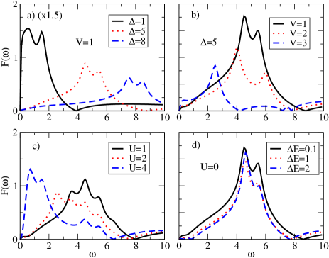
Figure 2: The relative non-Markovian spectrum $F(\omega)$ of the WTD. The parameters used for the four panels are given as follows. Upper left panel (a): $U=0$, $\Delta E=0$, $V=1.0$, $\Delta=1.0,5.0,8.0$. Upper right panel (b): $U=0$, $\Delta E=0$, , $\Delta=5.0$. $V=1.0,2.0,5.0$. Bottom left panel (c): $\Delta E=0$, $V=1.0$, $\Delta=5.0$ , $U=1.0,2.0,4.0$. Bottom right panel (d): $V=1.0$, $\Delta=5.0$ , $U=0.0$, $\Delta E=0.1,1.0,2.0$.

Figure 2 shows the relative non-Markovian spectrum of the WTD represented by

$$F(\omega)=\frac{1}{\Gamma}\frac{|P(\omega)-P^{(0)}(\omega)|}{P^{(0)}(\omega)}.$$ (26)

It is noteworthy that $F(\omega)$ is independent of the system reservoir coupling strength parameter $\Gamma$. The WDT spectrum reveals several frequencies that are present in the transient oscillations. These depend only on the internal transfer rate $\Delta$, Coulomb coupling $U$, and bias voltage $V$. The specific values of the parameters are given in the caption of the figure. Figure 2(a) shows the main characteristics of $F(\omega)$, consisting of two overlapping sub-peaks centered around the value of $\Delta$. Changing the value of $\Delta$ leads to the shift of both sub-peaks equally by $\Delta$. In Fig. 2(b), $\Delta$ is kept constant and the bias voltage is varied. We find that the splitting of the two sub-peaks is determined by the applied voltage. Labeling the two peaks with $\pm$, respectively, we can deduce the following relation for the corresponding characteristic frequencies. $\omega_{\pm}=|\Delta\pm V/2|$. In the presence of Coulomb interaction, we observe an additional double–peaks feature at $|U-\Delta\pm V/2|$, as demonstrated in Fig. 2(c). This is similar to a non-Markovian shot noise spectrum,Jin et al. (2008) where a finite Coulomb interaction $U$ induces also additional peaks due to the energy gap between the two-particle occupation state and lower states. On the other hand, the orbital detuning does not induce additional peaks in the double quantum dot in series as shown in Fig. 2(d).

Oscillations of Rabi frequency, which were observed in parallel DQD systems,Welack et al. (2008a, 2009); Brandes (2008) are however absent in the present series DQD system. In the parallel cases, the transport proceeds via two channels, and the Rabi oscillations in the WDT can be observed as the consequence of quantum mechanical interferences.Welack et al. (2008a, 2009); Brandes (2008) It is also noted that the information contained in the spectrum of the non-Markovian WDT is mostly equivalent to a measurement of the non-Markovian shot noise spectrum. For this purpose, the WTD can be considered as an alternative approach to the shot noise spectrum measurement.

IV.2 Memory landscape of consecutive waiting times

The expansion in non-Markovian corrections, Eq. (25), can be readily employed to calculate the two propagators involved in the two-times joint probabilities defined by Eq. (21). Denote

$$Q^{(n)}(\tau_{2},\tau_{1}) =\sum_{k=0}^{n}\sum_{j=0}^{n}\langle\langle G^{(k)}(\tau_{2}-\tau_{1})W^{(r-)}$$

$$\qquad\ \ \times G^{(j)}(\tau_{1}-t_{0})W^{(l+)}\bm{p}(t_{0})\rangle\rangle.$$ (27)

A memory landscape of the system can be calculated by the difference between non-Markovian and Markovian two-times joint probabilities

$$L^{(n)}(\tau_{2},\tau_{1})=\frac{Q^{(n)}(\tau_{2},\tau_{1})-Q^{(0)}(\tau_{2},\tau_{1})}{Q^{(0)}(\tau_{2},\tau_{1})}.$$ (28)

The order $n$ of the perturbative expansion in non-Markovian corrections has to be chosen in accordance to the parameters in order to assure satisfactory convergence. We find that the summation to the fourth non-Markovian contribution already converges sufficiently for the given parameters. As the memory in Eq. (28) decays, the relative non-Markovian landscape $L^{(n)}(\tau_{2},\tau_{1})$ converges to zero. Figure 3 shows the memory landscape of two survival times related to two consecutive electron transfers through the left electrode. It visualizes how memory of the waiting time $\tau_{1}$ after the first transfer is carried over into the waiting time $\tau_{2}$ following the second transfer.

We find that the non-Markovian effects are small for the given parameters in case the DQD is coupled symmetrically to the electrodes. This is due to the relatively weak coupling of the DQD to the electrodes which is required in present counting experiment in order to resolve single electron transfers on the measurable timescales. It is observed that a stronger coupling to only one electrode induces significantly larger non-Markovian effects as shown in the left panels of Fig. 3.

In general, fast electron transfers are necessary in order to observe significant non-Markovian effects. The deviations for $\tau_{1}$, $\tau_{2}$ approaching zero from the Markovian value are due to the truncation of the transients in the derivation of the expansion. The expansion follows the general trend of a numerically exact solution. Both solutions overlap after the transients have decayed. However this causes relatively large inaccuracies for $\tau_{1}$ and $\tau_{2}$ close to zero.

There is an interesting dependency of the non-Markovian effects in the memory landscape on the Coulomb repulsion $U$. By comparing the upper panels of Fig. 3 where Coulomb repulsion is absent, with the bottom one, where a large $U$ induces a Coulomb blockade regime, we observe that memory decays faster with $\tau_{2}$ in the Coulomb blockade regime. This can be explained as follows. In the second regime, only a single electron can occupy the DQD and the double occupancy state does not provide memory for the second survival time leading to an overall smaller non-Markovian contribution. In this case, only one possible trajectory in the left to right direction is possible. An electron enters the unoccupied DQD at time $\tau_{1}=0$ and leaves it at time $\tau_{2}=0$.

The memory is preserved during $\tau_{1}$ by the single electron inside the DQD. However, after the electron has left a junction, the memory of its trajectory is lost rapidly since no other electron can serve as a messenger inside the DQD thus leading to comparatively short survival times $\tau_{2}$ where memory is present. In the regime where Coulomb repulsion is neglectible, a second electron can occupy the junction along the described trajectory, which is represented in the model by the presence of an occupied double occupancy state. The presence of the second electron preserves the memory during $\tau_{2}$ after the other electron has left the junction.

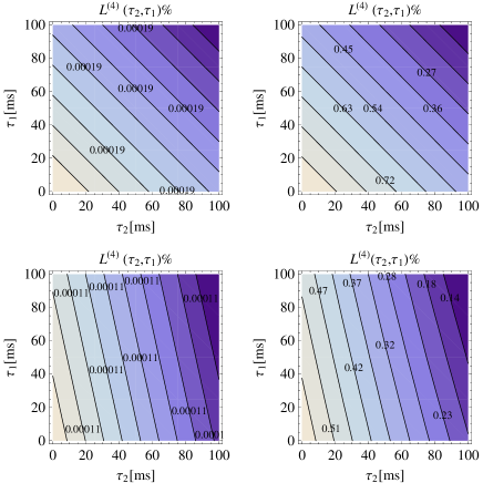
Figure 3: $L^{(4)}_{l,r}$ memory landscape of consecutive survival times. The bandwidth is large and a finite bias of $V=0.1k_{b}T$ is applied. The left coupling strength is $\Gamma^{(l)}=10^{4}Hz$. The upper panels are calculated in absence of Coulomb coupling, $U=0$, bottom panels display the Coulomb blockade regime, $U=\infty$. Left panels are calculated for a symmetric system, $\Gamma^{(l)}=\Gamma^{(r)}$. In the right panels, a stronger coupling strength is applied to the right electrodes $\Gamma^{(r)}=10^{6}Hz$.

V Conclusion

We find that non-Markovian effects are small in the regimes of recent single electron counting experiments. The sampling rate of current experiments is slow, a requirement which is imposed by the detection process of single electron transfers with currently available technology. This verifies the reason that the Markovian approximation of previous studies considering FCS or WTD is reasonable for the previously investigated systems.

Non-Markovian effects in the electron transfer statistics have to be taken into consideration for stronger electrode-DQD couplings, which then also requires faster sampling rates or a strongly asymmetric system. For example they affect the decay rates of the WTD which are directly related to the electronic structure of the system in junction.Welack et al. (2008b) Non-Markovian effects also induce several oscillations with characteristic system frequencies.

Note that the form of Pauli rate equation remains valid itself in the strong coupling limit. In the present paper we employ a perturbative approach to the rate equation and observe that the non-Markovian effects increase with the coupling strength. This observation is expected to remain true based on general Pauli rate equation dynamics. In other words, the non-Markovian effects are mainly visible for stronger couplings.

The employed microscopic non-Markovian rate equation provides a general framework to study similar systems and allows us to distinguish between non-Markovian effects due to intrinsic properties of the system, finite electrode-system coupling band-width and small bias voltages. It can be combined with quantum chemistry calculations that can calculate the employed parameters for molecules and their binding to the electronic bands of the metal electrodes. The approaches derived for the non-Markovian WTD are general and can be applied to a variety of processes in physics, chemistry and biology that are described by rate equations.

Appendix A Rate coefficients

Introducing the coupling reservoir spectrum density $J_{\alpha}(\omega)=\pi\sum_{q}|T^{(\alpha)}_{q}|^{2}\delta(\omega-\epsilon_{\alpha q})$ and applying Fermi statistics to the reservoir modes, the correlation functions (5) and (6) can be written as

$$C_{\alpha}^{(\pm)}(t)=\int_{-\infty}^{\infty}\frac{\mathrm{d}\omega}{\pi}\,J_{\alpha}(\omega)\,f_{\alpha}^{(\pm)}(\omega)e^{\mp i\omega t}.$$ (29)

Here, $f_{\alpha}^{(+)}(\omega)=1-f_{\alpha}^{(-)}(\omega)=[1+e^{\beta(\omega-\mu_{\alpha})}]^{-1}$ is the Fermi distribution function, with $\beta=1/k_{b}T$ being the inverse temperature and $\mu_{\alpha}$ the chemical potential of to the $\alpha$–electrode. Adopting a Lorentzian form of spectral density,

$$J_{\alpha}(\omega)=\gamma^{2}_{\alpha}/[(\omega-\Omega_{\alpha})^{2}+\gamma_{\alpha}^{2}],$$ (30)

the finite spectral width parameter $\gamma_{\alpha}$ is used to characterize the non-Markovian nature of system–reservoir coupling. With the complex roots of the Fermi function and of the Lorentzian spectral density, the integrals in Eq. (29) can be determined by the residues of the Kernel. The resulting infinite series are

$$C_{\alpha}^{(+)}(t)=\gamma_{\alpha}f_{\alpha}^{(+)}(\Lambda_{\alpha})e^{i\Lambda t}-\frac{2i}{\beta}\sum_{k=1}^{m}J_{\alpha}(\upsilon_{k})e^{i\upsilon_{k}t}$$ (31)

and

$$C_{\alpha}^{(-)}(t)=\gamma_{\alpha}f_{\alpha}^{(-)}(-\Lambda_{\alpha}^{\ast})e^{-i\Lambda^{\ast}t}-\frac{2i}{\beta}\sum_{k=1}^{m}J_{\alpha}(\upsilon_{k}^{\ast})e^{-i\upsilon_{k}^{\ast}t},$$ (32)

with the abbreviation $\Lambda_{\alpha}=\Omega_{\alpha}+i\gamma_{\alpha}$ and $\upsilon_{k}=\mu_{\alpha}+i\varpi_{k}$, where $\varpi_{k}\equiv(2k-1)\pi/\beta$ are the Fermion Matsubara frequencies. In order to completely separate real and imaginary parts of the correlation functions (5) and (6), we first separate its individual components. For the two complex Fermi functions we calculate

$$f_{\alpha}^{(\pm)}(\pm\Omega_{\alpha}+i\gamma_{\alpha})=\frac{1+e^{\pm\beta(\Omega_{\alpha}-\mu_{\alpha})}e^{-i\beta\gamma_{\alpha}}}{X^{\pm}_{\alpha}},$$ (33)

where

$$X^{\pm}_{\alpha}\equiv 1+2\cos(\beta\gamma_{\alpha})e^{\pm\beta(\mu_{\alpha}-\Omega_{\alpha})}+e^{\pm 2\beta(\mu_{\alpha}-\Omega_{\alpha})}.$$ (34)

The complex spectral densities can be separated into

$$\quad J_{\alpha}(\mu_{\alpha}\pm i\varpi_{k})$$

$$=\frac{[\varpi_{k}^{2}+(\mu_{\alpha}-\Omega_{\alpha})^{2}+\gamma_{\alpha}^{2}]\mp 2i\varpi_{k}(\mu_{\alpha}-\Omega_{\alpha})}{Y_{\alpha}},$$ (35)

where

$$Y_{\alpha}\equiv\frac{1}{\gamma^{2}_{\alpha}}[\varpi_{k}^{2}+(\mu_{\alpha}-\Omega_{\alpha})^{2}+\gamma_{\alpha}^{2}]^{2}+4\varpi_{k}^{2}(\mu_{\alpha}-\Omega_{\alpha})^{2}.$$ (36)

Based on the separation in real and imaginary contributions, we can write the correlation functions as

$$C_{\alpha}^{(\pm)}(t) =(a_{\alpha}^{\pm}+ib_{\alpha}^{\pm})e^{(\pm i\Omega_{\alpha}-\gamma_{\alpha})t}$$

$$\quad+\sum_{k=1}^{m}(c_{\alpha k}^{\pm}+id_{\alpha k}^{\pm})e^{(\pm i\mu_{\alpha}-\varpi_{k})t}.$$ (37)

The coefficients are all real:

$$a_{\alpha}^{\pm} =\frac{\gamma_{\alpha}}{X^{\pm}_{\alpha}}[1+e^{\pm\beta(\Omega_{\alpha}-\mu_{\alpha})}\cos(\beta\gamma_{\alpha})],$$ (38a)

$$b_{\alpha}^{\pm} =\frac{\gamma_{\alpha}}{X^{\pm}_{\alpha}}[e^{\pm\beta(\Omega_{\alpha}-\mu_{\alpha})}\sin(\beta\gamma_{\alpha})],$$ (38b)

$$c_{\alpha k}^{\pm} =\mp\frac{4(\mu_{\alpha}-\Omega_{\alpha})\varpi_{k}}{\beta Y_{\alpha}},$$ (38c)

$$d_{\alpha k}^{\pm} =\mp\frac{2[\varpi_{k}^{2}+(\mu_{\alpha}-\Omega_{\alpha})^{2}+\gamma_{\alpha}^{2}]}{\beta Y_{\alpha}}.$$ (38d)

Rigorously, the sum over the Matsubara values would be infinite; i.e., $k_{\rm max}=m\rightarrow\infty$ in Eqs. (31) and (32), but it can be truncated for practical purposes at a finite value that depends on the temperature of the system $T$ and the spectral width.

References

- Lu et al. (2003) W. Lu, Z. Ji, L. Pfeiffer, K. W. West, and A. J. Rimberg, Nature 423, 422 (2003).
- Fujisawa et al. (2004) T. Fujisawa, T. Hayashi, Y. Hirayama, H. D. Cheong, and Y. H. Jeong, Appl. Phys. Lett. 84, 2343 (2004).
- Gustavsson et al. (2006) S. Gustavsson, R. Leturcq, B. Simovic, R. Schleser, T. Ihn, P. Studerus, K. Ensslin, D. C. Driscoll, and A. C. Gossard, Phys. Rev. Lett. 96, 076605 (2006).
- Fujisawa et al. (2006) T. Fujisawa, T. Hayashi, R. Tomita, and Y. Hirayama, Science 312, 1634 (2006).
- Levitov et al. (1996) L. S. Levitov, H. W. Lee, and G. B. Lesovik, J. Math. Phys. 37, 4845 (1996).
- Levitov and Reznikov (2004) L. S. Levitov and M. Reznikov, Phys. Rev. B 70, 115305 (2004).
- Wabnig et al. (2005) J. Wabnig, D. V. Khomitsky, J. Rammer, and A. L. Shelankov, Phys. Rev. B 72, 165347 (2005).
- Rammer et al. (2004) J. Rammer, A. L. Shelankov, and J. Wabnig, Phys. Rev. B 70, 115327 (2004).
- Shelankov and Rammer (2003) A. L. Shelankov and J. Rammer, Europhys. Lett. 63, 485 (2003).
- Flindt et al. (2005) C. Flindt, T. Novotny, and A.-P. Jauho, Europhys. Lett. 69, 475 (2005).
- Utsumi et al. (2006) Y. Utsumi, D. S. Golubev, and G. Schoen, Phys. Rev. Lett. 96, 086803 (2006).
- Pedersen and Wacker (2005) J. N. Pedersen and A. Wacker, Phys. Rev. B 72, 195330 (2005).
- Bachtold et al. (2001) A. Bachtold, P. Hadley, T. Nakanishi, and C. Dekker, Science 294, 1317 (2001).
- Kießlich et al. (2006) G. Kießlich, P. Samuelsson, A. Wacker, and E. Schöll, Phys. Rev. B 73, 033312 (2006).
- Engel and Loss (2004) H.-A. Engel and D. Loss, Phys. Rev. Lett. 93, 136602 (2004).
- Braggio et al. (2006) A. Braggio, J. König, and R. Fazio, Phys. Rev. Lett. 96, 026805 (2006).
- Braggio et al. (2008) A. Braggio, C. Flindt, and T. Novotný, Physica E 40, 1745 (2008).
- Flindt et al. (2008) C. Flindt, T. Novotny, A. Braggio, M. Sassetti, and A.-P. Jauho, Phys. Rev. Lett. 100, 150601 (2008).
- Brandes (2008) T. Brandes, Ann. Phys. 17, 477 (2008).
- Welack et al. (2008a) S. Welack, M. Esposito, U. Harbola, and S. Mukamel, Phys. Rev. B 77, 195315 (2008a).
- Koch et al. (2005) J. Koch, M. Raikh, and F. v. Oppen, Phys. Rev. Lett. 95, 056801 (2005).
- Welack et al. (2008b) S. Welack, J. B. Maddox, M. Esposito, U. Harbola, and S. Mukamel, Nano Lett. 8, 1137 (2008b).
- Welack et al. (2009) S. Welack, S. Mukamel, and Y. J. Yan, EPL 85, 57008 (2009).
- Zaidi (2006) H. Zaidi, Phys. Rev. A 73, 061802 (2006).
- Jin et al. (2008) J. S. Jin, X. Q. Li, and Y. J. Yan, arXiv:0806.4759 (2008).
- Weiss (1999) U. Weiss, Quantum Dissipative Systems (World Scientific, Singapore, 1999), 2nd ed. Series in Modern Condensed Matter Physics, Vol. 10.
- Yan and Xu (2005) Y. J. Yan and R. X. Xu, Annu. Rev. Phys. Chem. 56, 187 (2005).
- Welack et al. (2006) S. Welack, M. Schreiber, and U. Kleinekathöfer, J. Chem. Phys. 124, 044712 (2006).