Collapse of differentially rotating supermassive stars: Post black hole formation

Abstract

We investigate the collapse of differentially rotating supermassive stars (SMSs) by means of 3+1 hydrodynamic simulations in general relativity. We particularly focus on the onset of collapse to understand the final outcome of collapsing SMSs. We find that the estimated ratio of the mass between the black hole (BH) and the surrounding disk from the equilibrium star is roughly the same as the results from numerical simulation. This suggests that the picture of axisymmetric collapse is adequate, in the absence of nonaxisymmetric instabilities, to illustrate the final state of the collapse. We also find that quasi-periodic gravitational waves continue to be emitted after the quasinormal mode frequency has decayed. We furthermore have found that when the newly formed BH is almost extreme Kerr, the amplitude of the quasi-periodic oscillation is enhanced during the late stages of the evolution. Geometrical features, shock waves, and instabilities of the fluid are suggested as a cause of this amplification behaviour. This alternative scenario for the collapse of differentially rotating SMSs might be observable by LISA.

I Introduction

There exists plenty of evidence that supermassive black holes (SMBHs) exist in the centre of galaxies, but their actual formation process has been a mystery for many decades (Rees, 2003). Several different scenarios have been proposed, some based on stellar dynamics, others on gas hydrodynamics, and still others that combine these processes. There are three major routes to form a SMBH. One possibility is that the gas in the newly-forming galaxy does not break up into stellar-mass condensations, but instead forms a single superstar, and then undergoes complete gravitational collapse. Another possibility is that instead of forming a single superstar, black holes (BHs) might grow from smaller seeds, and then merge to form a SMBH. The final possibility is the runaway growth of a stellar mass BH to a SMBH by accretion. Here we consider the possibility of forming a SMBH from the collapse of a supermassive star (SMS).

There are two categories of collapsing rotating SMSs based on their angular momentum distribution. One is the collapse of a uniformly rotating SMS. This happens when momentum transport is large, either through viscous turbulence or magnetic processes, which drives the star to rotate uniformly. In this case the path to the SMBH is the following. First the SMS contracts until the mass shedding limit is reached, conserving the angular momentum of the star. If the SMS contains sufficient angular momentum, the star evolves quasi-stationary along the mass-shedding limit, releasing the mass and angular momentum. When the star reaches the post-Newtonian instability it begins to collapse. Baumgarte and Shapiro (1999) found that the star starts to collapse from the universal configuration when the system contains sufficient angular momentum, independent of the history of the star. Saijo et al. (2002) found that the collapse is coherent. That is, no significant bar instability occurs before BH formation in three dimensional post-Newtonian simulations. Shibata and Shapiro (2002) found that a final Kerr BH of $a/M\approx 0.75$ contains 90% of the total rest-mass of the system, and that the disk around the BH contains 10% of that in an axisymmetric general relativistic simulation.

The other category of collapsing rotating SMSs are differentially rotating. This happens when the viscous and the magnetic effects are small, which allows the star to rotate differentially. One of the representative scenarios for forming a differentially rotating star is as follows. First, a gas cloud gathers in an almost spherical configuration with some amount of angular momentum in the system. Next the almost spherical star contracts, conserving specific angular momentum due to the lack of viscosity, to form a differentially rotating star, and possibly a disk at the end of the contraction (Bodenheimer and Ostriker, 1973).

During the contraction of the differentially rotating SMS, prior to forming a supermassive disk, two possible instabilities may arise that terminate the contraction. One is the post-Newtonian gravitational instability, which leads the star to collapse dynamically. The other is the dynamical bar mode instability, which changes the angular momentum distribution of the star to form a bar, and possibly leads to the central core of the star collapsing to a BH due to the angular momentum loss.

One of the primary observational missions for space-based detection of gravitational waves is the investigation of supermassive objects ((, 1998)). Since the Laser Interferometer Space Antenna (LISA) will have long arms ($10^{6}\,{\rm km}$), the detector will be most sensitive in the low frequency band ($10^{-4}\sim 10^{-1}$ Hz). Potential sources of high signal to noise events in this frequency range include quasi-periodic waves arising from nonaxisymmetric bars in collapsing SMSs and the inspiral of binary SMBHs (e.g. Ref. ((, 2009))). In addition, the nonspherical collapse of rotating SMSs to SMBHs could be a significant source of burst and quasi-normal gravitational waves (e.g. Ref. ((, 2003))). In this paper we track the collapse of a SMS by numerical simulation to investigate some of these possibilities.

Figure 1: Maximum of the rest mass density as a function of time. Solid, dashed, dotted, and dash-dotted lines denote models I, II, III, IV, respectively.

Here we focus on the post-Newtonian gravitational instability in differentially rotating SMSs. The aim of this work is to understand the final fate of the collapse of differentially rotating SMSs. There are two studies that address this issue. New and Shapiro (2001) studied the “zero-viscosity” equilibrium sequence in differentially rotating SMSs in Newtonian gravity. They showed that the star reaches the bifurcation point of dynamical bar instability before the disk forms by contraction. Saijo (2004) studied the gravitational collapse of differentially rotating SMSs in the conformally flat approximation of general relativity near the onset of radial instability. He showed that once the star collapses, the collapse is coherent and may form a SMBH with no substantial nonaxisymmetric deformation due to instability. However the previous work may contain less angular momentum so that there might be no significant difference between the cases of uniform rotation and differential rotation. Therefore we now focus on the case where the angular momentum is more contained in the star than the previous case, which potentially leads to rotational instabilities if they occur. In particular, we plan to answer the following questions. Does the BH form coherently? What are the features of the dynamics? Does the newly formed disk lead to instabilities? Can this system act as an efficient source of gravitational waves (GWs)? In order to answer these questions, three dimensional general relativistic hydrodynamics are desirable.

The content of this paper is as follows. In Sec. II, we briefly explain the general relativistic hydrodynamics, especially the numerical tools we used to simulate the violent phenomena. In Sec. III, we introduce our findings of dynamical BHs, disk formation, and gravitational waves. Section IV is devoted to the summary of this paper. Throughout this paper, we use the geometrized units with $G=c=1$ and adopt Cartesian coordinates $(x,y,z)$ with the coordinate time $t$. Note that Greek index takes $(t,x,y,z)$, while Latin one takes $(x,y,z)$.

II Basic equations

In this section, we briefly describe the three-dimensional relativistic hydrodynamics in full general relativity.

II.1 The gravitational field equations

We define the spatial projection tensor $h^{\mu\nu}\equiv g^{\mu\nu}+n^{\mu}n^{\nu}$, where $g^{\mu\nu}$ is the spacetime metric, $n^{\mu}=(1/\alpha,-\beta^{i}/\alpha)$ the unit normal to a spatial hypersurface, and where $\alpha$ and $\beta^{i}$ are the lapse and shift. Firstly, we introduce a conformal factor $\psi=e^{\phi}$ to the spatial three metric $\gamma_{ij}$ as

$$\tilde{\gamma}_{ij}=e^{-4\phi}\gamma_{ij},$$ (1)

and choose the determinant of the conformally related metric $\tilde{\gamma}_{ij}$ to be unity, $\phi=(\ln\gamma)/12$. Secondly, we introduce a trace-free part of the extrinsic curvature $A_{ij}$, and its conformally related tensor $\tilde{A}_{ij}$, whose indices will be raised and lowered by the conformally related metric $\tilde{\gamma}_{ij}$, as in Ref. (Shibata and Nakamura, 1995),

$$\tilde{A}_{ij}=e^{-4\phi}A_{ij}=e^{-4\phi}\left(K_{ij}-\frac{1}{3}\gamma_{ij}K\right),$$ (2)

where $K_{ij}$ is the extrinsic curvature. Finally we introduce the conformal connection functions $\tilde{\Gamma}^{i}$ (Baumgarte and Shapiro, 1998)

$$\tilde{\Gamma}^{i}\equiv\tilde{\gamma}^{jk}\tilde{\Gamma}^{i}_{jk}=-\frac{\partial}{\partial x^{j}}\tilde{\gamma}^{ij},$$ (3)

as a variable to describe the Ricci tensor of the conformally related metric. This step, the expansion of the Ricci tensor in terms of the metric based variables, plays a crucial role in maintaining a long time stable evolution of Einstein’s field equations (Shibata and Nakamura, 1995).

Table 1: Four different rotating equilibrium SMSs for evolution

Model	spacetime	$R_{\rm p}/R_{\rm e}$	$\rho_{0}^{\rm max}$	$M$	$T/W$	$J/M^{2}$	$M/R$	$m_{\rm disk}$	$(a/M)^{\rm(BH)}$
I	GR	$0.450$	$1.56\times 10^{-5}$	$4.88$	$0.108$	$0.99$	$2.56\times 10^{-2}$	—	—
I	CF	$0.450$	$1.56\times 10^{-5}$	$4.88$	$0.108$	$0.99$	$2.56\times 10^{-2}$	$0.044$	$0.98$
II	GR	$0.425$	$1.56\times 10^{-5}$	$5.07$	$0.118$	$1.03$	$2.63\times 10^{-2}$	—	—
II	CF	$0.425$	$1.56\times 10^{-5}$	$5.07$	$0.118$	$1.03$	$2.63\times 10^{-2}$	—	$\gtrsim 1$
III	GR	$0.400$	$1.56\times 10^{-5}$	$5.31$	$0.131$	$1.07$	$2.78\times 10^{-2}$	—	—
IV	GR	$0.375$	$1.56\times 10^{-5}$	$5.75$	$0.156$	$1.10$	$3.47\times 10^{-2}$	—	—

Therefore we evolve the spacetime with the 17 spacetime associated variables ($\phi$, $K$, $\tilde{\gamma}_{ij}$, $\tilde{A}_{ij}$, $\tilde{\Gamma}^{i}$) as

$$\left(\frac{\partial}{\partial t}-{\cal L}_{\beta}\right)\phi = -\frac{1}{6}\alpha K,$$ (4)

$$\left(\frac{\partial}{\partial t}-{\cal L}_{\beta}\right)K = -\gamma^{ij}D_{i}D_{j}\alpha+\alpha\left[\tilde{A}_{ij}\tilde{A}^{ij}+\frac{1}{3}K^{2}+\frac{1}{2}(\rho_{\rm H}+S)\right],$$ (5)

$$\left(\frac{\partial}{\partial t}-{\cal L}_{\beta}\right)\tilde{\gamma}_{ij} = -2\alpha\tilde{A}_{ij},$$ (6)

$$\left(\frac{\partial}{\partial t}-{\cal L}_{\beta}\right)\tilde{A}_{ij} = e^{-4\phi}[-D_{i}D_{j}\alpha+\alpha(R_{ij}-S_{ij})]^{\rm TF}+\alpha(K\tilde{A}_{ij}-2\tilde{A}_{il}\tilde{A}^{l}_{j}),$$ (7)

$$\left(\frac{\partial}{\partial t}-{\cal L}_{\beta}\right)\tilde{\Gamma}^{i} = -2\tilde{A}^{ij}\frac{\partial}{\partial x^{j}}\alpha+2\alpha\left(\tilde{\Gamma}^{i}_{jk}\tilde{A}^{jk}-\frac{2}{3}\tilde{\gamma}^{ij}\frac{\partial}{\partial x^{j}}K-\tilde{\gamma}^{ij}S_{j}+6\tilde{A}^{ij}\frac{\partial}{\partial x^{j}}\phi\right)$$ (8)

$$-\frac{\partial}{\partial x^{j}}\left(\beta^{l}\frac{\partial}{\partial x^{l}}\tilde{\gamma}^{ij}-2\tilde{\gamma}^{m(j}\frac{\partial}{\partial x^{m}}\beta^{i)}+\frac{2}{3}\tilde{\gamma}^{ij}\frac{\partial}{\partial x^{l}}\beta^{l}\right),$$

where ${\cal L}_{\beta}$ denotes the Lie derivative along the shift $\beta^{i}$, $\rho_{\rm H}=T_{\mu\nu}n^{\mu}n^{\nu}$, $S_{i}=T_{\mu\nu}n^{\mu}h^{\nu}_{i}$ and TF the trace-free part of the tensor. This set of equations when used to solve Einstein’s field equations numerically is usually called the BSSN formalism.

We use as a slicing condition the generalised hyperbolic $K$-driver (Alcubierre et al., 2003; Pollney et al., 2007)

$$\left(\frac{\partial}{\partial t}-\beta^{i}\frac{\partial}{\partial x^{i}}\right)\alpha=-\alpha^{2}f(\alpha)(K-K_{0}),$$ (9)

where $f(\alpha)=2/\alpha$, $K_{0}=K_{t=0}$ in order to avoid singularities. As for the shift, we use the generalised hyperbolic $\tilde{\Gamma}$-driver (Baker et al., 2006)

$$\left(\frac{\partial}{\partial t}-\beta^{j}\frac{\partial}{\partial x^{j}}\right)\beta^{i} = \frac{3}{4}\alpha B^{i},$$ (10)

$$\left(\frac{\partial}{\partial t}-\beta^{j}\frac{\partial}{\partial x^{j}}\right)B^{i} = \left(\frac{\partial}{\partial t}-\beta^{j}\frac{\partial}{\partial x^{j}}\right)\tilde{\Gamma}^{i}-\eta B^{i},$$

where $\eta$ is a damping parameter.

Figure 2: Hamiltonian constraint (solid line) and Momentum constraints (dashed lines) for models I and II throughout the evolution. Note that we normalised $HC$ with $16\pi\rho_{\rm max}$ and $MC_{i}$ with $8\pi\rho_{\rm max}\sqrt{M/R}$, where $M$ is the gravitational mass, $R$ the circumferential radius of the equilibrium star, respectively.

II.2 The matter equations

For a perfect fluid, the energy momentum tensor takes the form

$$T^{\mu\nu}=\rho\left(1+\varepsilon+\frac{P}{\rho}\right)u^{\mu}u^{\nu}+Pg^{\mu\nu},$$ (12)

where $\rho$ is the rest-mass density, $\varepsilon$ the specific internal energy, $P$ the pressure, $u^{\mu}$ the four-velocity.

We adopt a $\Gamma$-law equation of state in the form

$$P=(\Gamma-1)\rho\varepsilon,$$ (13)

where $\Gamma$ is the adiabatic index which we set to $4/3$ in this paper, representing a SMS (the pressure is dominated by radiation).

In the absence of thermal dissipation, Eq. (13), together with the first law of thermodynamics, implies a polytropic equation of state

$$P=\kappa\rho^{1+1/n},$$ (14)

where $n=1/(\Gamma-1)$ is the polytropic index and $\kappa$ a constant.

From $\nabla_{\mu}T^{\mu\nu}=0$ together with the continuity equation, the flux conservative form of the relativistic continuity, the relativistic energy and the relativistic Euler equations are (Banyuls et al., 1997)

$$\frac{1}{\sqrt{-g}}\frac{\partial}{\partial t}(\sqrt{\gamma}{\boldsymbol{\cal U}})+\frac{1}{\sqrt{-g}}\frac{\partial}{\partial x^{i}}(\sqrt{-g}{\boldsymbol{\cal F}}^{i})=\boldsymbol{\cal S}^{i},$$ (15)

where the state vector $\boldsymbol{\cal U}$, the flux vectors $\boldsymbol{\cal F}^{i}$, and the source vectors $\boldsymbol{\cal S}^{i}$ are

$$\boldsymbol{\cal U} = [D,S_{i},\tau]^{T},$$ (16)

$$\boldsymbol{\cal F}^{i} = \left[D\left(v^{i}-\frac{\beta^{i}}{\alpha}\right),S_{j}\left(v^{i}-\frac{\beta^{i}}{\alpha}\right)+P\delta^{i}_{j},\tau\left(v^{i}-\frac{\beta^{i}}{\alpha}\right)+Pv^{i}\right]^{T},$$ (17)

$$\boldsymbol{\cal S}^{i} = \left[0,T^{\mu\nu}\left(\frac{\partial}{\partial x^{\mu}}g_{\nu j}-\Gamma^{\delta}_{\nu\mu}g_{\delta j}\right),\alpha\left(T^{\mu 0}\frac{\partial}{\partial x^{\mu}}\ln\alpha-T^{\mu\nu}\Gamma^{0}_{\nu\mu}\right)\right]^{T}.$$ (18)

Note that $(\rho,v_{i},\varepsilon)$ are the physical variables of the above equations, and the conserved quantities $D$, $S_{i}$, $\tau$ are

$$D = \rho W,$$ (19)

$$W = \alpha u^{t},$$ (20)

$$S_{i} = \rho hW^{2}v_{i},$$ (21)

$$E = \rho hW^{2}-P,$$ (22)

$$\tau = E-D,$$ (23)

where $v_{j}=u_{j}/W$, $h\equiv 1+\varepsilon+P/\rho$ is the specific enthalpy. In the Newtonian limit, the above three physical variables coincide to the rest mass density, the flux density of the rest mass, and the energy of a unit volume of fluid.

Figure 3: Rest mass, ADM mass and the total angular momentum throughout the evolution. We do not plot the above three quantities after the apparent horizon formation. Solid, dashed, dotted and dash-dotted line denote model I, II, III and IV, respectively. Since we use a different computational domain for computing a equilibrium and evolution quantities, the relative amount rate of $\approx 0.5\%$ appears in the ADM mass.

Figure 4: Centre of mass throughout the evolution. Solid and dash line denotes models I and II, respectively.

II.3 Dynamical horizon

A dynamical horizon is defined as the spacelike marginally trapped tube which is composed of future-marginally trapped surfaces on which the expansion associated with the ingoing null direction is strictly negative (Ashtekar and Krishnan, 2003). If it is the outermost trapped surface, which is expected to be the case with all those considered here, then it is an apparent horizon. An angular momentum of the horizon $J_{\rm BH}$ can be written (see e.g. section III.B of Ref. (Schnetter, Krishnan and Beyer, 2006)) as

$$J_{\rm BH}=-\frac{1}{8\pi}\int_{S_{\rm R}}K_{\mu\nu}R^{\mu}\varphi^{\nu}ds,$$ (24)

where $R^{\mu}$ is the outward directed spacelike normal to the horizon within the spacelike slice, and $\varphi^{a}$ is a rotational vector field on the horizon. This can be interpreted as the Komar angular momentum when $\varphi^{a}$ is a rotational Killing vector on the horizon. The code and method used to compute numerically an approximate Killing vector, should it exist, is described in Ref. (Dreyer et al., 2003).

The dynamical horizon mass of the hole $M_{\rm BH}$ can be computed once we have the angular momentum of the hole as

$$M_{\rm BH}=\frac{1}{2R_{\rm s}}\sqrt{R_{\rm s}+4J_{\rm BH}^{2}}.$$ (25)

Note that $R_{\rm s}$ is the area radius of the hole. We also monitor the dimensionless Kerr parameter $(J/M^{2})_{\rm BH}$ throughout the evolution.

II.4 Gravitational waveform

In order to monitor gravitational waves, we use the Newman-Penrose-Weyl scalar $\Psi_{4}$

$$\Psi_{4}=C_{\mu\nu\lambda\sigma}k^{\mu}\bar{m}^{\nu}k^{\lambda}\bar{m}^{\sigma},$$ (26)

where $C_{\mu\nu\lambda\sigma}$ is the Weyl tensor, $k^{\mu}$ the ingoing null vector, $m^{\mu}$ and $\bar{m}^{\mu}$ are the orthogonal spatial-null vectors of the four complex null tetrad ($l^{\mu}$, $k^{\mu}$, $m^{\mu}$, $\bar{m}^{\mu}$). More precisely, a set of null vectors are defined by introducing a orthonormal tetrad $e^{\mu}_{(a)}$ as

$$l^{\mu} = \frac{1}{\sqrt{2}}\left(e_{(0)}^{\mu}+e_{(1)}^{\mu}\right),$$ (27)

$$k^{\mu} = \frac{1}{\sqrt{2}}\left(e_{(0)}^{\mu}-e_{(1)}^{\mu}\right),$$ (28)

$$m^{\mu} = \frac{1}{\sqrt{2}}\left(e_{(2)}^{\mu}+ie_{(3)}^{\mu}\right),$$ (29)

$$\bar{m}^{\mu} = \frac{1}{\sqrt{2}}\left(e_{(2)}^{\mu}-ie_{(3)}^{\mu}\right).$$ (30)

Note that we choose the vector $e^{\mu}_{(0)}$ as the unit normal to the spatial hypersurface, $e^{\mu}_{(1)}$ the unit radial vector in spherical coordinates, and ($e^{\mu}_{(2)}$, $e^{\mu}_{(3)}$) the unit vectors in the angular directions. The Weyl scalar $\Psi_{4}$ represents the outgoing gravitational waves at infinity

$$\Psi_{4}=\ddot{h}_{+}-i\ddot{h}_{\times},$$ (31)

where $h_{+}$ and $h_{\times}$ are the two polarization modes (transverse-traceless condition) of the perturbed metric from flat spacetime in spherical coordinate and $\dot{q}$ represents the time derivative of the quantity $q$. If we put the observer sufficiently far from the source, the Weyl scalar $\Psi_{4}$ roughly represents the outgoing gravitational waves, ignoring the radiation back scattered by the curvature. Therefore we monitor the Weyl scalar $\Psi_{4}$ to understand key features of the gravitational waves emitted by this system.

II.5 Treatment of the spacetime singularity from the newly formed black hole

When a horizon is found in the simulation some of the matter within the horizon is excised from the domain using the technique of Ref. (Hawke, Löffler and Nerozzi, 2005). The domain excised is a sphere with coordinate radius half the minimum coordinate radius of the horizon at the time of excision. It is allowed to grow during evolution but not to shrink (in coordinate radius). Although the spacetime is not excised, we introduce a strong artificial dissipation term in Eqs. (4) – (LABEL:eqn:gauge_B), combined with the standard gauge conditions, to avoid problems with the singularity (Baiotti and Rezzolla, 2006). In practice, we add a dissipation term $-\epsilon dx^{i}\partial_{i}^{4}q$ in Eqs. (4) – (LABEL:eqn:gauge_B), where $q$ is the quantity evolved by the particular evolution equation. We specify the dissipation parameter $\epsilon\approx 0.2$ for our simulation.

In addition to this dissipation term, we have found it necessary to stabilize our evolutions in certain circumstances by reducing the timestep on individual refinement levels. This is particularly true for the finest levels near the horizon where low density matter is orbiting at extreme speed.

Figure 5: Contours of the rest mass density in the equatorial plane for model I. Snapshots are plotted at values of ($t$, $\rho_{\rm max}$) = (a) ($0$, $1.56\times 10^{-5}$), (b) ($671M$, $5.04\times 10^{-2}$), (c) ($755M$, $5.28\times 10^{-5}$) and (d) ($839M$, $1.68\times 10^{-5}$), with a cutoff density of $\rho_{\rm cut}=1.56\times 10^{-13}$, respectively. The contour lines denote rest mass densities $\rho/\rho_{\rm max}=10^{-(15-i)d}$ ($i=1,\cdots,14$), where $d=(\log\rho_{\rm max}-\log\rho_{\rm cut})/15$. Note that the apparent horizon exists after $t=671M$, and the coordinate radius of the apparent horizon in the equatorial plane are $r_{\rm hrz}=$ (c) $0.283M$ and (d) $0.417M$, respectively.

II.6 Computational codes and techniques

We perform 3+1 hydrodynamic simulations in general relativity using CACTUS (Goodale et al., 2003) (gravitational physics), CARPET (Schnetter, Hawley and Hawke, 2004) (mesh refinement of space and time), WHISKY (Baiotti et al., 2005) (see Ref. (Baiotti, Giacomazzo and Rezzolla, 2008) and references therein for a recent description) (general relativistic hydrodynamics). We set the outermost boundary of the computational grid for all direction as $x_{\rm max}=111$ – $131M$, imposing plane symmetry across the $z=0$ plane, and use 5 – 11 refinement levels to maintain the resolution at the central core region. We set the $i$-th refinement level of the uniform grid as $L_{i}=2^{7-i}\times 10$, $\Delta r_{i}=2^{5-i}$ ($i=1,\cdots,11$ for collapsing objects), where $L_{i}$ is the outer boundary of the grid, $\Delta r_{i}$ is the stepsize of the spatial grid, respectively. The finest central resolution for the collapsing SMS is $\Delta x=(3.08$ – $3.21)\times 10^{-3}M$. The Courant condition is set as $\Delta t=C_{\rm crt}\Delta x$, where $C_{\rm crt}=0.05$, $0.1$, $0.2$ for the finest three refinement levels for collapsing stars and $C_{\rm crt}=0.4$ for the rest of the refinement levels, damping parameter of the shift condition $\eta=3.91$ – $4.05$ $M^{-1}$ for the collapsing stars. As in previous works we use a reconstruction-evolution method to evolve the matter, with PPM reconstruction (Collela and Woodward, 1984) of the matter variables and Marquina’s formula (Aloy, Ibàñez, and Martí, 1999) to compute the inter-cell fluxes. Third order Runge-Kutta evolution in time is also used in our computation.

III Numerical Results

III.1 Equilibrium Stars

We construct the four differentially rotating SMSs for evolution. We use the polytropic equation of state of Eq. (14) with $n=3$, which represents the radiation pressure dominant, SMS sequence, and the relativistic “$j$-constant” rotation law as

$$u^{t}u_{\varphi}=A^{2}(\Omega_{c}-\Omega),$$ (32)

where $A(\equiv R_{e}\hat{A})$ represents the degree of differential rotation and has the dimension of length, $\Omega_{c}$ the central angular velocity, and $\Omega$ the angular velocity. We choose $\hat{A}=0.3$ here. In the Newtonian limit ($u^{t}\rightarrow 1$, $u_{\varphi}\rightarrow\varpi^{2}\Omega$ where $\varpi$ is the cylindrical radius of the star), this rotation law becomes

$$\Omega=\frac{A^{2}\Omega_{c}}{\varpi^{2}+A^{2}}.$$ (33)

We use the technique of Ref. (Stergioulas and Freidman, 1995) to construct the rotating equilibrium stars. Our four differentially rotating equilibrium stars that will be evolved using the full $\Gamma$-law equation of state of Eq. (13) are summarised in Table 1.

III.2 Disk Mass from Equilibrium Configuration

Before computing the collapse of the star, we can estimate the final rest mass ratio between BH and its surrounding materials with the technique of Ref. (Shibata and Shapiro, 2002). The idea is the following. Suppose a star collapses axisymmetrically throughout the system. In this case the rest mass $m_{*}$ and the angular momentum $j_{*}$ along each cylinder

$$m_{*} = \int_{V_{\rm cyl}}dv\sqrt{-g}\rho u^{t},$$

$$j_{*} = \int_{V_{\rm cyl}}dv\sqrt{-g}\rho u^{t}hu_{\varphi},$$

are, in the absence of viscosity, conserved throughout the evolution. Note that $V_{\rm cyl}$ is the three dimensional spatial volume along the cylinder. After the BH has formed, the material is swallowed at least up to the radius of the innermost stable circular orbit (ISCO) of the newly formed BH. Ignoring material from outside the ISCO we can approximate the rest mass of the BH, the angular momentum of the BH and the rest mass of the disk, defined as the mass outside the apparent horizon of the newly formed BH, as

$$m_{*}^{\rm BH} = \int_{V_{\rm isco}}dv\sqrt{-g}\rho u^{t},$$ (34)

$$j_{*}^{\rm BH} = \int_{V_{\rm isco}}dv\sqrt{-g}\rho u^{t}hu_{\varphi},$$ (35)

$$m_{*}^{\rm disk} = \int_{V_{\rm whl}-V_{\rm isco}}dv\sqrt{-g}\rho u^{t},$$ (36)

where $V_{\rm isco}$ is the three dimensional spatial volume inside the cylindrical radius of ISCO, $V_{\rm whl}$ the whole three dimensional spatial volume, and $V_{\rm whl}-V_{\rm isco}$ is the three dimensional spatial volume outside the ISCO cylindrical radius in each hypersurface.

In practise, we compute the specific angular momentum at ISCO $j_{\rm isco}$. Note that $j\equiv hu_{\varphi}$ is a monotonic growing quantity as a function of cylindrical radius, and that $j_{\rm isco}$ is a function of the cylindrical rest mass $m_{*}$ and the approximate, dimensionless Kerr parameter $j_{*}/m_{*}^{2}$. If there is a maximum in $j_{\rm isco}$ as a function of the cylindrical rest mass (cylindrical radius), the quantities at the maximum (cylindrical rest mass and specific angular momentum) correspond to the quantity of the newly formed BH if the equilibrium star collapses. After the determination of the cylindrical rest mass of the BH, we can compute that of the disk from the total rest mass of the system. We can also compute the approximate Kerr parameter from the quantities at the maximum. To simplify the calculation our estimates of the ratio between disk mass and the BH mass and the Kerr parameter are computed in conformally flat spacetime (using the methods of e.g. Ref. (Saijo, 2004)) and are summarised in Table 1.

Figure 6: Same as Fig. 5, but in the meridional plane.

Figure 7: Contours of the rest mass density in the equatorial plane for model II. Snapshots are plotted at values of ($t$, $\rho_{\rm max}$) = (a) ($0$, $1.56\times 10^{-5}$), (b) ($768M$, $5.07\times 10^{-2}$), (c) ($849M$, $1.05\times 10^{-4}$) and (d) ($930M$, $6.12\times 10^{-5}$), with a cutoff density of $\rho_{\rm cut}=1.56\times 10^{-13}$, respectively. The contour lines denote rest mass densities $\rho/\rho_{\rm max}=10^{-(15-i)d}$ ($i=1,\cdots,14$), where $d=(\log\rho_{\rm max}-\log\rho_{\rm cut})/15$. Note that the apparent horizon exists after $t=770M$, and the coordinate radius of the apparent horizon in the equatorial plane are $r_{\rm hrz}=$ (c) $0.170M$ and (d) $0.175M$, respectively.

Figure 8: Same as Fig. 7, but in the meridional plane.

III.3 Collapse of Differentially Rotating Supermassive Stars

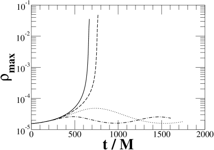
We first investigate the onset of collapse by evolving the four differentially rotating equilibrium stars of Table 1. We choose the $z$-axis as the rotational one of the equilibrium star. Since we use the polytropic equation of state $P=\kappa\rho_{0}^{\Gamma}$ ($P$: pressure, $\kappa$: constant, $\rho_{0}$: rest mass density, $\Gamma$: adiabatic exponent) when constructing initial data sets, all physical quantities are rescalable in terms of $\kappa$. Therefore, we represent all physical quantities nondimensionally in this paper, which is equivalent to setting $\kappa=1$. To trigger collapse, we deplete pressure by 1%. Checking the maximum rest mass density of the rotating stars throughout the evolution, we conclude that models I and II are radially unstable, while models III and IV are stable (Fig. 1).

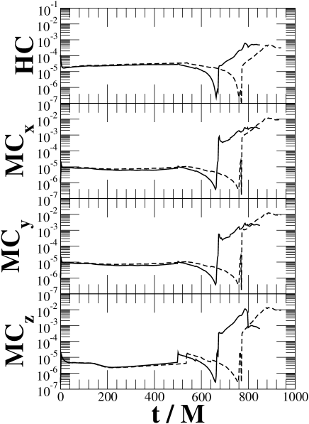
Since we use a free evolution scheme for the 17 variables associated with the spacetime, the constraint equations of Einstein’s field equations are not automatically satisfied at each timestep. Therefore we can monitor the Hamiltonian constraint and Momentum constraints as a check on the accuracy of the simulation. We define them as

$$HC = R-K^{i}_{\;\;j}K^{j}_{\;\;i}+K^{2}-16\pi\rho_{\rm H},$$ (37)

$$MC_{i} = \nabla_{j}K_{i}^{\;\;j}-\nabla_{i}K-8\pi S_{i},$$ (38)

and show them for models I and II in Fig. 2. Since these quantities should be exactly zero sense, we normalise the Hamiltonian constraint by $16\pi\rho_{\rm max}$ and the Momentum constraints by $8\pi\rho_{\rm max}\sqrt{M/R}$, where $\rho_{\rm max}$ is the maximum rest mass density at each timestep. Both of the normalisation quantities represent the typical size of the source term of the constraints (maximum rest-mass density and collapsing momentum density). Since all constraint quantities are conserved within $\approx$1% from Fig. 2, the constraints seem to be satisfied at a reasonable level throughout the evolution.

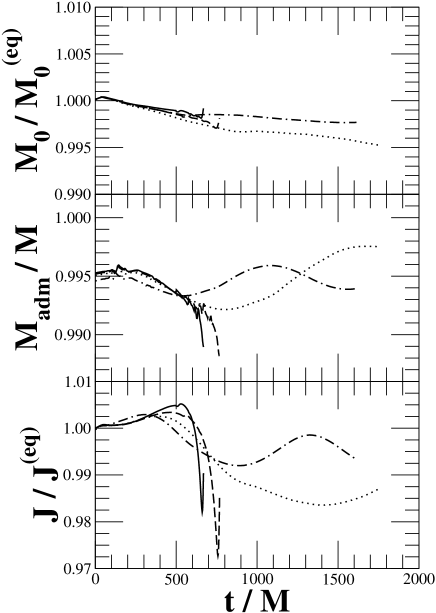
We also monitor the rest mass $M_{0}$, ADM mass $M_{\rm adm}$, and the total angular momentum $J$

$$M_{0} = \int dv\rho u^{t}\sqrt{-g},$$

$$M_{\rm adm} = -\frac{1}{2\pi}\oint_{\infty}\nabla^{i}\psi dS_{i}$$

$$= \int[(\rho hW^{2}-P)e^{5\phi}+\frac{1}{16\pi}e^{5\phi}A_{ij}A^{ij}],$$

$$J = \frac{1}{8\pi}\oint_{\infty}(x\tilde{A}_{yj}-y\tilde{A}_{xj})e^{6\phi}dS^{j}$$

$$= \int dve^{6\phi}[xS_{y}-yS_{x}+\frac{1}{8\pi}(\tilde{A}^{x}_{y}-\tilde{A}^{y}_{x})$$

$$-\frac{1}{16\pi}\tilde{A}_{ij}(x\partial_{y}-y{\partial}_{x})\tilde{\gamma^{ij}}$$

$$+\frac{1}{12\pi}(x\partial_{y}-y{\partial}_{x})K^{k}_{k}],$$

throughout the evolution in Fig. 3. We only monitor these three quantities until the time when the apparent horizon forms, since our excision method significantly complicates the computation of the required volume integrals after horizon formation. From Fig. 3, $M_{0}$ is conserved to within $0.5\%$, $M_{\rm adm}$ to within $1\%$, and $J$ to within $2\%$. Therefore, we can conclude that all three quantities are satisfactory conserved for our case.

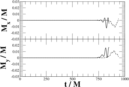
We also monitor the centre of mass condition in Fig. 4. In practise we monitor

$$M_{x} = \frac{\int dv^{\rm(half)}\rho x}{M_{0}^{\rm(half)}},$$ (39)

$$M_{y} = \frac{\int dv^{\rm(half)}\rho y}{M_{0}^{\rm(half)}},$$ (40)

where $M_{0}^{\rm(half)}$ is the rest mass of $z\geq 0$, $dv^{\rm(half)}$ the spatial volume of $z\geq 0$, since we adopt planar symmetry across $z=0$. Since our finest spatial gridsize is $\approx 3\times 10^{-3}M$, the centre of mass motion is contained within a few finest grids cells from the origin. Therefore, we can conclude that centre of mass condition is satisfied for our case.

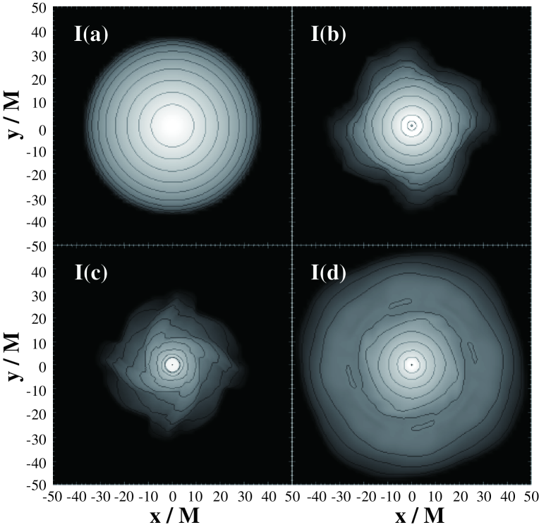
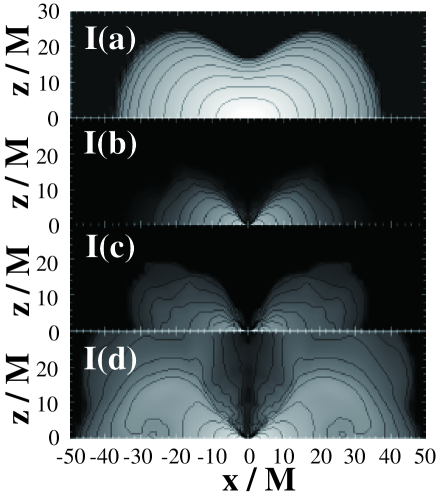
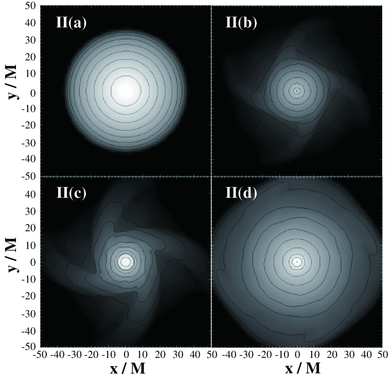
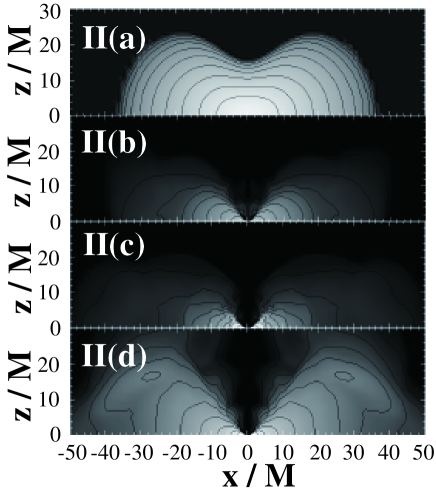
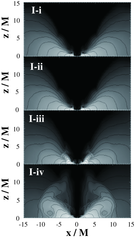
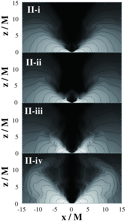
We show contours of the rest mass density in Figs. 5 (equatorial plane) and 6 (meridional plane) for model I and in Figs. 7 (equatorial plane) and 8 (meridional plane) for model II. As we can easily understand from these figures, the radially unstable stars first collapse to form a BH. After that, there is a significant amount of mass ejection due to the large amount of angular momentum of the hole. It is indeed like a flare. Finally the system settles down to a quasi-stationary state; central BH with a disk. Fluid elements in the equilibrium star are balanced by its self gravity, the pressure gradient and centrifugal force. When the BH forms, some fluid elements act as a particle which is free from the interaction. In this case, the material can spread out to a larger radius than the equilibrium radius of the star. Note that there seem to have $m=4$ structure in the snapshots of I (b) (c) (Fig. 5) and II (c) (Fig. 7). We believe that this is due to the reduced spatial computational resolution of the outer regions of the star (See Ref. (Saijo, 2004) for a different resolution case).

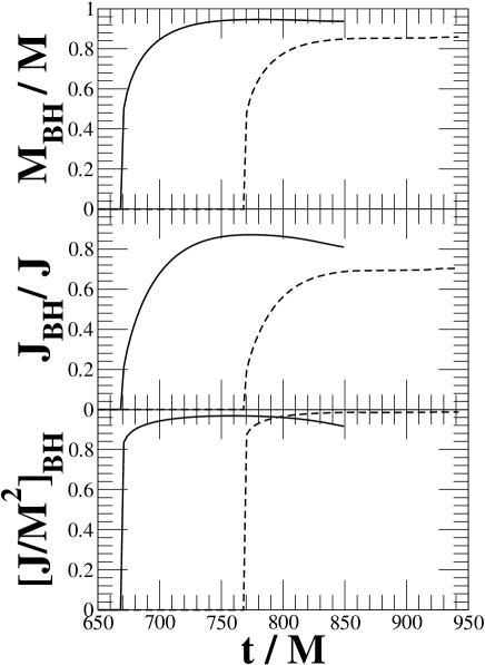
Next we trace the mass and the angular momentum of the newly formed BH throughout the evolution using the dynamical horizon techniques outlined in Sec. II.3. We monitor the gravitational mass, total angular momentum and the Kerr parameter of the newly formed BH throughout the evolution as shown in Fig. 9. The BH mass, the spin and the Kerr parameter increase monotonically after the BH has formed, by swallowing much of the surrounding material. This stage lasts roughly until all of the matter located inside the radius of the innermost stable circular orbit of the final BH is swallowed.

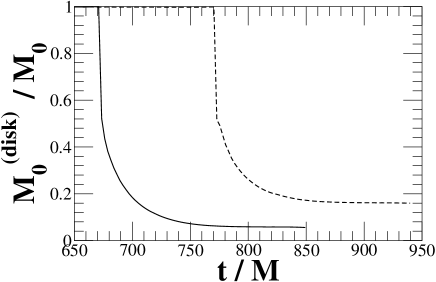
We have also confirmed that the estimated mass and spin of the BH from the equilibrium configuration of the collapsing SMS are in good agreement with the results from the dynamics. Although we calculated the disk mass from the equilibrium configuration in conformally flat spacetime, there is a little difference in the physical quantities between full general relativistic spacetime and conformally flat spacetime (see Table 1). For instance, the estimated Kerr parameter from the equilibrium star of model I is $0.98$ (Table 1), while the result of numerical simulation is $\approx 0.97$ (Fig. 9). Also the ratio between the estimated rest mass of the disk and the rest mass of the equilibrium star of model I is $0.044$ (Table 1), while the result of numerical simulation is $\approx 0.05$ (Fig. 10). Note that we define the rest mass of the disk as the rest mass outside the apparent horizon in each timeslice.

We furthermore study the formation of a massive disk from the collapse of differentially rotating SMSs. We trace the rest mass of the disk for models I and II (Fig. 10). The rest mass of the disk monotonically decreases once the BH has formed, since the newly formed BH grows monotonically by swallowing the surrounding materials. One noticeable feature in Fig. 10 is that there is a plateau at the final stage of model II. This indicates that there is a strong angular momentum barrier that a fluid fragments are prohibited to fall into a hole. We also illustrate the snapshot of the rest mass density in the meridional plane of model II (Fig. 8 II[d]). The maximum of the rest mass density is located around $r\approx 2M$ in coordinate units.

Figure 9: Gravitational mass ($M_{\rm BH}$), total angular momentum ($J_{\rm BH}$) and Kerr parameter ($(J/M^{2})_{\rm BH}$) of a newly formed BH as a function of time. Solid and dashed line represent models I and II, respectively.

Figure 10: Disk mass as a function of time. We defined the disk mass as the rest mass outside the apparent horizon of the newly formed BH. Solid and dashed line represent models I and II, respectively.

Figure 11: $m=1$ and $m=2$ diagnostics of the ring in the equatorial plane throughout the collapse for model I. We monitor the diagnostics at the coordinate radius $r=1.02M$ (upper two panels) and $2.05M$ (lower two panels), respectively. Note that the solid line and the dashed line denote $m=1$ and $m=2$. The coordinate equatorial radius of the horizon at $t=854M$ is $r=0.464M$.

Figure 12: Same as Fig. 11, but we monitor the diagnostics at the coordinate radius $r=4.1M$ (upper two panels) and $10.2M$ (lower two panels), respectively.

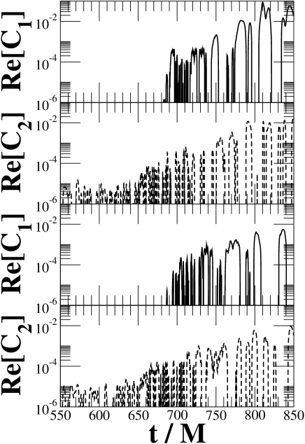
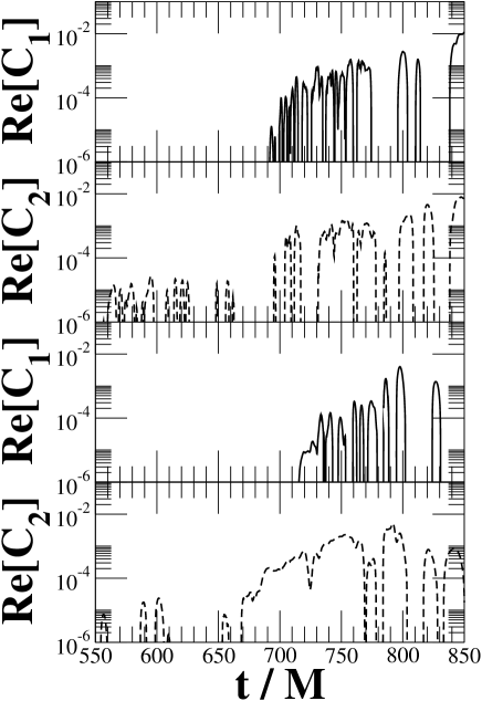
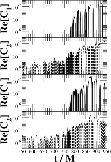
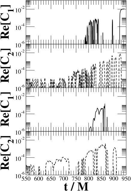
We also monitor the diagnostics of the $m=1$ and $m=2$ Fourier modes throughout the collapse in Figs. 11 and 12 (for model I) and Figs. 13 and 14 (for model II). We define the diagnostics $C_{m}$ as

$$C_{m}=\frac{1}{2\pi}\int_{0}^{2\pi}\rho e^{im\varphi}d\varphi,$$ (41)

with a normalisation of $C_{0}$, a mean density of the ring. In order to understand the characteristic frequency, we also show the spectrum of the ring diagnostics $|{\cal F}[\rho_{m}](\omega)|^{2}$ using the Fourier transformation as

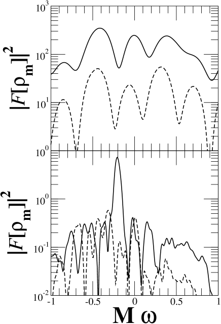
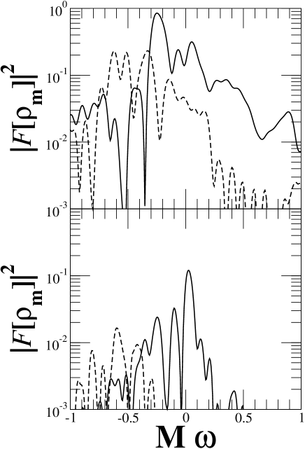
$${\cal F}[\rho_{m}](\omega)=\frac{1}{4\pi^{2}}\int_{0}^{t_{\rm fin}}dt\int_{0}^{2\pi}\rho e^{i(\omega t-m\varphi)}d\varphi,$$ (42)

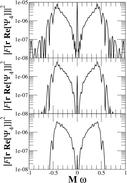
where $t_{\rm fin}$ is the time where we terminate our simulation. We show the spectra of the $m=1$ and $m=2$ diagnostics in Figs. 15 and 16.

The diagnostics show that non-axisymmetries (that would be triggered at least at the level of finite-differencing error through the simulation) do not grow to meaningful levels near the centre of the system until well past horizon formation. When these non-axisymmetries appear, they grow rapidly before saturating. From the growth of the coefficients at larger radius, shown in Figs. 12 and 14, it seems clear that the non-axisymmetries are triggered in the interior of the disk and propagate outwards.

Figure 13: $m=1$ and $m=2$ diagnostics throughout the collapse for models II. We monitor the diagnostics at $r=0.197M$ (upper two panels) and $0.987M$ (lower two panels), respectively. Note that the solid line and the dashed line denote $m=1$ and $m=2$. The coordinate equatorial radius of the horizon at $t=940M$ is $r=0.177M$.

Figure 14: Same as Fig. 13, but we monitor the diagnostics at $r=3.95M$ (upper two panels) and $9.87M$ (lower two panels), respectively.

Figure 15: Spectra of $m=1$ and $m=2$ diagnostics throughout the collapse for model I. The top panel is monitored at the coordinate radius $r=1.02M$, while the bottom panel $r=2.05M$. Note that the solid line and the dashed line denote $m=1$ and $m=2$.

Figure 16: Spectra of $m=1$ and $m=2$ diagnostics throughout the collapse for model II. The top panel is monitored at the coordinate radius $r=0.197M$, while the bottom panel $r=0.987M$. Note that the solid line and the dashed line denote $m=1$ and $m=2$.

III.4 Gravitational radiation

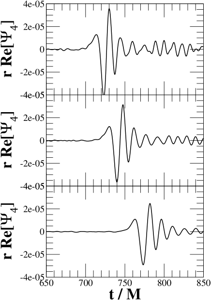
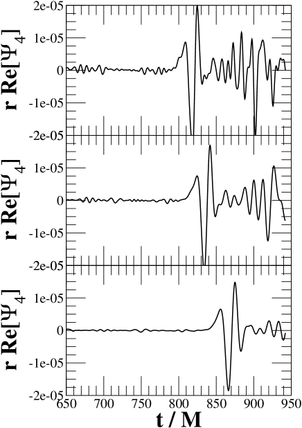
Finally we investigate the gravitational waveform from the collapsing object. We introduce the Weyl scalar $\Psi_{4}$ to study the outgoing gravitational waves. If we put the observer sufficiently far from the source, the Weyl scalar $\Psi_{4}$ roughly represents the outgoing gravitational waves, since the radiation back scattered by the curvature behaves as $r^{-3}$, where $r$ is the distance from the source. We observe the waveform (the real component of $\Psi_{4}$) along the $x$-axis in the equatorial plane at three different coordinate locations with radius $r\approx 50M$, $\approx 65M$, $\approx 100M$ for models I and II (Figs. 17 and 18). Note that the equatorial coordinate radius of the equilibrium star is $r=38.1M$ and $37.0M$, and the outermost boundary of the spatial grid is $131M$ and $126M$, for models I and II.

We find that the waveform contains three different stages. The first stage is the burst. This occurs around the time when the apparent horizon of the SMS forms. The dominant contribution of the burst comes from the axisymmetric mode due to collapse. The second stage is the quasinormal ringing of the newly formed BH. Since the dominant frequency in the spectrum (Figs. 19 and 20) is $M\omega\approx 0.4$, the dominant contribution is the axisymmetric one, using the fact that quasinormal mode frequency of $l=2$, $m=0$ is $M\omega\approx 0.40$ – $0.42$ for a BH with Kerr parameter $a\gtrsim 0.8M$ Leaver (1985), where $l$, $m$ denotes the indices of spin $-2$-weighted spheroidal harmonics. The final stage has a quasi-stationary wave. The amplitude of the waveform for model II seems to increase at late times. The feature corresponds to several peaks in the spectrum (Fig. 20), especially in the regime of $M\omega\lesssim 0.5$. For model I, the quasi-stationary waveform remains for at least $\Delta t\sim 70M$ (Fig. 20). In this case the spectra does not contain the peaks in the regime of $M\omega\lesssim 0.5$. When we reduce the integration time of the quasi-periodic waves (comparing the three panels in Fig. 20), the spectrum becomes much smoother in the frequency regime $M\omega\gtrsim 0.5$. Therefore the frequency region of $M\omega\gtrsim 0.5$ plays a role in the quasi-periodic waveform. Although we do not know the origin of the late-time quasi-periodic waves, we can discuss possible candidates and their likelihood.

Figure 17: Gravitational waveform measured with the Weyl scalar $\Psi_{4}$ observed along the $x$-axis in the equatorial plane at $r=49.14M$ (top panel), $r=65.52M$ (middle panel) and $98.29M$ (bottom panel) for model I. Note that the time at which the apparent horizon is first detected is $t=670M$. Taking the wave propagation time from the source to the observer into account, the apparent horizon formation in the waveform is roughly just before the peak due to the burst. Initially a standard burst and ringdown signal are seen (compare (Buonanno, Cook and Pretorius, 2007), especially their Fig. 18), but sustained gravitational wave emission indicate additional dynamics after BH formation.

Figure 18: Gravitational waveform measured with the Weyl scalar $\Psi_{4}$ observed along the $x$-axis in the equatorial plane at $r=47.36M$ (top panel), $r=63.15M$ (middle panel) and $94.72M$ (bottom panel) for model II. Note that the time at which the apparent horizon is first detected is $t=770M$. Taking the wave propagation time from the source to the observer into account, the apparent horizon formation in the waveform is roughly just before the peak due to the burst.

Figure 19: Spectra of the real part of the Weyl scalar $\Psi_{4}$ observed along the $x$-axis in the equatorial plane at $r=49.14M$ (top panel), $r=65.52M$ (middle panel) and $98.29M$ (bottom panel) for model I.

Figure 20: Spectra of the Weyl scalar $\Psi_{4}$ observed along the $x$-axis in the equatorial plane at $r=47.36M$ (top panel), $r=63.15M$ (middle panel) and $94.72M$ (bottom panel) for model II.

Figure 21: Contours of the rest mass density in the meridional plane for model I. Snapshots are plotted at values of ($t$, $\rho_{\rm max}$) = i ($713M$, $1.87\times 10^{-4}$), ii ($734M$, $1.24\times 10^{-4}$), iii ($755M$, $5.28\times 10^{-5}$) and iv ($776M$, $2.87\times 10^{-5}$), with a cutoff density of $\rho_{\rm cut}=1.56\times 10^{-13}$, respectively. The contour lines denote rest mass densities $\rho/\rho_{\rm max}=10^{-(15-i)d}$ ($i=1,\cdots,14$), where $d=(\log\rho_{\rm max}-\log\rho_{\rm cut})/15$. Note that the apparent horizon exists after $t=671M$, and the coordinate radius of the apparent horizon in the equatorial plane are $r_{\rm hrz}=$ i $0.295M$, ii $0.282M$, iii $0.283M$ and iv $0.297M$, respectively. Shocks can be found in the snapshots of I-ii.

Figure 22: Contours of the rest mass density in the meridional plane for model II. Snapshots are plotted at values of ($t$, $\rho_{\rm max}$) = i ($808M$, $3.15\times 10^{-4}$), ii ($828M$, $1.88\times 10^{-4}$), iii ($849M$, $1.05\times 10^{-4}$) and iv ($869M$, $4.85\times 10^{-5}$), with a cutoff density of $\rho_{\rm cut}=1.56\times 10^{-13}$, respectively. The contour lines denote rest mass densities $\rho/\rho_{\rm max}=10^{-(15-i)d}$ ($i=1,\cdots,14$), where $d=(\log\rho_{\rm max}-\log\rho_{\rm cut})/15$. Note that the apparent horizon exists after $t=770M$, and the coordinate radius of the apparent horizon in the equatorial plane are $r_{\rm hrz}=$ i $0.173M$, ii $0.167M$, iii $0.170M$ and iv $0.180M$, respectively. Shocks can be found in the snapshot of II-ii.

Figure 23: Angular velocity of circular orbit at ISCO radius as a function of Kerr parameter.

Firstly we distinguish between the different possibilities for the amplification of the waves based on the dominant type of behaviour. The most obvious possibility would be strong matter dynamics perturbing the essentially stationary Kerr spacetime given by the dominant central BH. The second possibility is a weaker, more indirect coupling, where either the matter dynamics in the disk lead to gravitational waves, or a global oscillation or resonance of whole spacetime exists, including both the exterior matter and the BH.

In the first category where the wave emission is dominated by the motion of the fluid in Kerr spacetime, there are two possibilities. One is that inhomogeneities or radial motion in the disk exist, leading to the wave emission. These can be viewed, to a first approximation, as small fluid fragments behaving approximately like test particles orbiting a Kerr BH. If we further approximate the “particle” to be moving in a circular orbit then the characteristic frequency $\omega_{\rm circular}$ and the amplitude $h_{\rm circular}$ from the quadrupole formula of gravitational waves can be written as

$$\omega_{\rm circular} = m\Omega_{r_{0}},$$ (43)

$$rh_{+~{}{\rm circular}} = 7\times 10^{-1}\mu(M\omega)^{3/2}\cos\omega t,$$ (44)

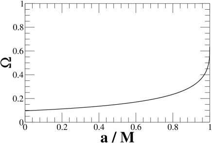
where $\Omega_{r_{0}}$ is the orbital angular velocity of the particle at the radius of ISCO $r_{0}$, and $r$ is the distance from the source. The typical frequency for a circular orbit can be also applied for the scattering particle at the innermost radius $r_{0}$. We show the relation between the orbital angular velocity at ISCO and the Kerr parameter in Fig. 23. In fact, when the newly formed BH is near extremal, the typical frequency $\omega_{\rm circular}$ and the amplitude $h_{+~{}{\rm circular}}$ of gravitational waves are

$$M\omega_{\rm circular} = M\Omega_{r_{0}}\approx 0.5,$$

$$rh_{+~{}{\rm circular}} \approx 2\times 10^{-5}M\left(\frac{M\omega}{0.5}\right)^{3/2},$$

assuming that the only contribution to the amplitude comes from the particle at ISCO (the ring mass is $\approx 3\times 10^{-5}$), and that $m=1$ is dominant ($\omega_{\rm circular}=\Omega_{r_{0}}$). For $m=1$ we have that $M\omega=M\Omega\approx 0.5$. This idea is suggested from the spectra of gravitational waveform (Figs. 19 and 20). At every observed radius, there is a peak around $M\omega\approx 0.5$, which might correspond to the motion of the particle at inner edge. However this idea cannot explain the enhancement of the quasi-periodic waves when the newly formed BH is almost extremal. We also note that the Fourier coefficients as shown in Figs. 11 – 14 show non-axisymmetries growing in the interior and moving out far too late (in retarded time) to cause the enhanced gravitational waves.

Remaining with the idea that the gravitational waves are generated by the fluid motion, we note that the dynamics of the matter as shown by Figs. 5 – 8 change after horizon formation. Initially all matter collapses in. However, once the quasi-stable disk forms in the interior there is still some infalling matter left, which “splashes” onto the disk. This is reminiscent of the centrifugal bounce seen in early core-collapse simulations with a simple equation of state (e.g. the Type II multiple-bounce models of Ref. (Dimmelmeier, Font and Müller, 2002)). As the rotation rate increases and the spacetime is near extreme Kerr, the chances of shocks appearing through some form of accretion are significantly increased, as shown as far back as Wilson (1972). After submission, we note that simulations of core collapse (Murphy, Ott and Burrows (2009)) have seen gravitational waves due to rapidly decelerated shocks. The shocks formed by the accreting matter could lead to wave-packet like bursts of gravitational waves. As these form in the outer layers of the disk and predominantly propagate out, their effects are never seen in the Fourier coefficients shown in Figs. 11 – 14. It is possible to approximately correlate the shocks appearing in Figs. 21 and 22 with the start of the quasi-periodic waves in Figs. 17 and 18. Rest-mass density snapshots in the meridional plane show that shock waves are generated around $t\approx 734M$ for model I and $t\approx 828M$ for model II. Quasi-periodic waves in $\Psi_{4}$ starts at $t\approx 780M$ at $r\approx 50M$ for model I, at $t\approx 870M$ at $r\approx 50M$ for model II. Since radiation propagates at speed of light, those times for each model roughly correspond with each other. However, it seems unlikely that these shocks could produce quasi-periodic waves of near constant amplitude as seen in model I, where the newly formed BH is not an extremal one (Fig. 17).

In the second category, we are looking for a property of the full spacetime including both the BH and the matter. As the Kerr BH contains the majority of the mass in the system, we would expect this to dominate. So either there must be some special property of quasi-normal modes of near extremal Kerr BHs, or there must be a coupling through the spacetime between the matter in the disk and the Kerr BH. Since we know that the imaginary part of the quasi-normal mode frequency goes to zero at extreme Kerr limit Sasaki and Nakamura (1989), there are long-lived modes for near-extremal Kerr BHs, and hence small perturbations from the exterior matter may produce long-lived gravitational wave signals such as those seen in Fig. 17 for model I. It is not clear that this could easily lead to the strong amplification seen for model II in Fig. 18.

A final possibility that we consider in this category is a corotation resonance. In fact when the spin of the newly formed BH is very close to extreme Kerr, the amplitude of the gravitational wave signal gradually grows after the quasinormal ringing. We also check the azimuthal $m$ modes of the rest mass density traced at the certain radius in the equatorial plane, and found that the $m=2$ mode starts growing exponentially after the ringdown (Fig. 16, second top panel). One possible explanation for the exponential growth of the $m=2$ mode at late times is the existence of corotation resonance of the newly formed disk triggered by the vibration of the hole. Note that the necessary condition to excite corotation resonance in fluid mechanics is $\omega_{\rm chr}=m\Omega$ (e.g. Ref. (Saijo and Yoshida, 2006)), where $\omega_{\rm chr}$ is the characteristic frequency of the system, $\Omega$ the angular velocity. If the corotation resonance is triggered by quasinormal ringing, the necessary condition for triggering a corotation resonance is $\omega_{\rm qnm}=m\Omega$ at a certain radius of the interior star. The real part of the quasi-normal mode frequency of $l=m=2$ increases with increasing Kerr parameter, and becomes $M\omega_{\rm qnm}=1$ for the extreme Kerr BH. The orbital velocity at ISCO also increases with increasing Kerr parameter, and becomes $M\Omega_{r_{0}}=(3-\sqrt{3})/2=m\omega_{\rm particle}$ for the extreme Kerr BH ($\omega_{\rm qnm}<m\omega_{\rm particle}$). Therefore, the condition $\omega_{\rm qnm}=m\omega_{\rm paricle}$ is satisfied for $m=2$ for a certain Kerr parameter near the extremal limit.

IV Conclusion

We have investigated the collapse of differentially rotating SMSs, especially focusing on the post BH formation stage, by means of three dimensional hydrodynamic simulations in general relativity. We particularly focus on the onset of collapse to form a rapidly rotating BH as a final outcome.

We have found that the qualitative results of the evolution for the mass and spin of the final BH and disk are quite similar to the estimates that can be computed from the equilibrium configuration when the estimated, final BH has $J_{\rm(BH)}/M_{\rm(BH)}^{2}<1$. This result suggests that in the absence of a nonaxisymmetric instability, the estimate of the BH mass and the disk mass agree with a simple axisymmetric picture that the specific angular momentum is conserved throughout the evolution, and the newly formed BH swallows the matter up to the radius of the ISCO.

We have also found that a quasi-periodic wave occurs after the ringdown of a newly formed BH. As we would normally expect the ringdown waveform to damp, it seems likely that the cause of this waveform is due to the presence of the disk in some form. Furthermore, when the newly formed BH is sufficiently close to extreme Kerr with sufficient surrounding matter we have found that the wavesignal may be significantly amplified.

We have discussed several possibilities for the origin of these amplified waves. The most likely possibilities seem to be (a) corotation resonance between the disk and the BH, (b) long-lived gravitational waves from the near-extreme BH amplified by perturbations in the disk, or (c) shocks from the infalling, accreting matter.

It may be possible to distinguish between some of these possibilities by further time integration, although at present the computational expense is prohibitive. The wave-packet or burst nature of waves generated by shocks, for example, should be possible to distinguish at later times and at larger radii of extraction. The slow power law decay ($\sim 1/t$) in the extremal limit (Andersson and Glampedakis, 2000) would, however, be difficult to accurately capture at present with this type of nonlinear numerical simulation. Alternatives to free evolution simulations such as the Fully Constrained Formalism of Refs. (Bonazzola et al., 2004; Cordero-Carrión et al., 2008) should significantly improve the accuracy and hence may be capable of capturing such effects, but the specific gauge currently required by this formalism may make it difficult to get a numerically well-behaved simulation of the extreme cases investigated here.

Additional information about the horizon geometry could be found from the multipole structure of the dynamical horizon (as defined in Ref. Ashtekar et al. (2004); various numerical implementations are discussed in Refs. Schnetter, Krishnan and Beyer (2006); Vasset et al. (2009); Jasiulek (2009); Owen (2009)). In particular this may indicate whether a strong perturbation of the BH geometry is connected to the gravitational waves seen here. However, it seems likely, comparing in particular to the results of Refs. Jasiulek (2009); Owen (2009) where long term evolutions of “clean” binary black hole systems are considered, that better numerical accuracy and longer integration times will be required in order to rule out any but the strongest of perturbations.

Finally we discuss the detectability of gravitational waves from this system. The characteristic strength $h$ and the frequency $f$ of the burst and ringing are (e.g. Ref. (Saijo et al., 2002))

$$f_{\rm burst} \sim 3\times 10^{-2}\left(\frac{10^{6}M_{\odot}}{M}\right)\left(\frac{M}{R}\right)^{3/2}[{\rm Hz}],$$ (45)

$$h_{\rm burst} \sim 1\times 10^{-18}\left(\frac{M}{10^{6}M_{\odot}}\right)\left(\frac{1{\rm Gpc}}{d}\right)\left(\frac{M}{R}\right),$$ (46)

$$f_{\rm QNM} \sim 2\times 10^{-2}\left(\frac{10^{6}M_{\odot}}{M}\right){\rm[Hz]},$$ (47)

$$h_{\rm QNM} \sim 6\times 10^{-19}\left(\frac{\Delta E_{\rm GW}/M}{10^{-4}}\right)^{1/2}\left(\frac{2\times 10^{-2}{\rm[Hz]}}{f_{\rm QNM}}\right)^{1/2}\left(\frac{M}{10^{6}M_{\odot}}\right)^{1/2}\left(\frac{1{\rm Gpc}}{d}\right),$$ (48)

where $d$ is the distance from the observer and $\Delta E_{\rm GW}$ is the total radiated energy. We set $R/M=1$, a characteristic mean radius during BH formation. Since the main targets of LISA are gravitational radiation sources between $10^{-4}$ and $10^{-1}$ Hz, it is possible that LISA can search for the burst and quasi-normal ringing waves accompanying rotating SMS collapse and formation of an SMBH. Moreover, the frequency of the quasi-periodic waves after the quasinormal ringing is quite similar to that of quasinormal ringing, so is in the detectable regime. Also the amplitude of the quasi-periodic wave is roughly $10\%$ of the burst at the horizon, and hence this feature can also be seen in LISA.

Although we focus on the case of the collapse of differentially rotating SMS to a SMBH in this paper, our model is also applicable to the collapse of population III stars which are also radiation pressure dominated. In this case, the mass range of the collapsing object becomes of the order of a few hundred solar masses. Therefore the most sensitive region for the detection of burst waves and quasinormal ringing waves becomes the order of hertz. Such gravitational waves might be seen in Deci-hertz interferometer gravitational wave observatory (DECIGO) (Kawamura et al., 2006).