Bayesian inference with an adaptive proposal density for GARCH models

Abstract

We perform the Bayesian inference of a GARCH model by the Metropolis-Hastings algorithm with an adaptive proposal density. The adaptive proposal density is assumed to be the Student’s t-distribution and the distribution parameters are evaluated by using the data sampled during the simulation. We apply the method for the QGARCH model which is one of asymmetric GARCH models and make empirical studies for for Nikkei 225, DAX and Hang indexes. We find that autocorrelation times from our method are very small, thus the method is very efficient for generating uncorrelated Monte Carlo data. The results from the QGARCH model show that all the three indexes show the leverage effect, i.e. the volatility is high after negative observations.

1 Introduction

In empirical finance volatility of asset returns is an important value to measure risk. In order to forecast future volatility it is desirable to use appropriate models which have the properties of volatility of asset returns. Many empirical studies suggest that the distribution of asset returns is leptokurtic. Furthermore the volatility is not constant, but changes over time. There are periods when volatility is very high or very low. This property of the volatility is called volatility clustering.

The Autoregressive Conditional Heteroscedasticity (ARCH) model[1] and its generalization, the Generalized ARCH (GARCH) model[2] are designed to capture the property of the volatility clustering. Moreover the distributions of returns from those models show fat-tailed distributions and they are suggested to be Student’s t-(Tsallis) distributions[3, 4]. There are many extensions of the GARCH model to include additional properties of the volatility. An example of the properties of the volatility is that the volatility response is high after negative news (returns), which is known as the leverage effect, first observed by Black[5]. In order to cope with this fact, some models[6, 7, 8, 9, 10, 11] which introduce asymmetry into the volatility response function are proposed. In this study among them we focus on the Quadratic GARCH(QGARCH) model[10, 11] which adds an additional term proportional to a return to the volatility response function.

To utilize the GARCH models we need to infer GARCH parameters from financial time series data. In general the Maximum Likelihood (ML) estimation is favored to the inference of GARCH models. Although implementation of the ML method is straightforward, there exist practical difficulties in estimating GARCH parameters by the ML technique. The model parameters must be positive to ensure a positive volatility and the stationarity condition for volatility is also required. The ML method with such requirements is performed via a constrained optimization technique which can be cumbersome. Forethermore the output of the ML method is often sensitive to starting values.

Another estimation technique is the Bayesian inference which does not have the difficulties seen in the ML method. Usually the Bayesian inference is performed by Markov Chain Monte Carlo (MCMC) methods which have been common in the recent computer development. Various MCMC methods for the Bayesian inference of the GARCH models have been proposed[12, 13, 14, 15, 16, 17, 18, 19]. In a survey on the MCMC methods of the GARCH models[17] it is shown that Acceptance-Rejection/ Metropolis-Hastings (AR/MH) algorithm with a multivariate Student’s t-distribution works better than the other algorithms. The multivariate Student’s t-distribution is used as a proposal density of the MH algorithm and the parameters to specify the Student’s t-distribution are determined by the Maximum Likelihood (ML) technique. Recently an alternative method to estimate those parameters without relying on the ML technique was proposed[20, 21, 22]. The method is called ”adaptive construction scheme”, where the parameters of the multivariate Student’s t-distribution are determined by using the pre-sampled data by an MCMC method. And the parameters are updated adaptively during the MCMC simulation.

The adaptive construction scheme was tested for GARCH and QGARCH models[20, 21, 22] and it is shown that the adaptive construction scheme can significantly reduce the correlation between sampled data. In this paper first we describe the adaptive construction scheme for the GARCH models. Then we make empirical studies with the QGARCH model for three major stock indexes, Nikkei 225, DAX and Hang Seng.

2 GARCH Model

Let $x_{t}$ be an asset return observed at time $t$. We transform $x_{t}$ to $y_{t}$ as

$$y_{t}=x_{t}-\bar{x},$$ (1)

where $\bar{x}$ is the average over $N$ observations, i.e. $\displaystyle\bar{x}=\frac{1}{N}\sum_{i=1}^{N}x_{i}$. In the GARCH model $y_{t}$ is assumed to be decomposed as

$$y_{t}=\sigma_{t}\epsilon_{t},$$ (2)

where $\epsilon_{t}$ is an identically distributed random variable with zero mean and unit variance. The distribution of $\epsilon_{t}$ is usually assumed to be a normal (Gaussian) or a leptokurtic one. In this study we assume that the distribution is a normal one, i.e. $\sim N(0,1)$. In the original GARCH model the volatility $\sigma_{t}$ is assumed to change over time as

$$\sigma_{t}^{2}=\omega+\sum_{i=1}^{q}\alpha_{i}y_{t-i}^{2}+\sum_{i=1}^{p}\beta_{i}\sigma_{t-i}^{2},$$ (3)

and more specifically this model is stated as the GARCH(p,q) model. Since in empirical studies with the AIC analysis small numbers are often chosen for $p$ and $q$ we focus on the GARCH(1,1) model in this study and write it as the GARCH model. Now eq.(3) is written as

$$\sigma_{t}^{2}=\omega+\alpha y_{t-1}^{2}+\beta\sigma_{t-1}^{2}.$$ (4)

The volatility response function of eq.(4) is symmetric under positive or negative observations $y_{t}$. However some asset returns are known to show the leverage effect, i.e. the volatility is higher after negative observations than after positive ones. Several extended GARCH models have been proposed to introduce asymmetry into the volatility response function. In this study we use the QGARCH model[10, 11] given by

$$\sigma_{t}^{2}=\omega+\gamma y_{t-1}+\alpha y_{t-1}^{2}+\beta\sigma_{t-1}^{2},$$ (5)

where the additional term, $\gamma y_{t-1}$ introduces the asymmetry into the model. The QGARCH model includes 4 parameters ($\omega,\alpha,\beta,\gamma$) which have to be determined from financial data.

3 Maximum Likelihood Estimation

The likelihood function of the GARCH models is written as

$$L(y|\theta)=\Pi_{i=1}^{n}\frac{1}{\sqrt{2\pi\sigma_{t}^{2}}}\exp\left.(-\frac{y_{t}^{2}}{2\sigma_{t}^{2}}\right.),$$ (6)

where $y$ stands for the time series data of $n$ observations, $y=(y_{1},....y_{n})$ and $\theta$ stands for GARCH parameters, e.g. for the QGARCH model $\theta=(\omega,\alpha,\beta,\gamma$).

In the ML estimation the parameters are determined by maximizing the log likelihood $\ln L(y|\theta)$,

$$\ln L(y|\theta)=-\frac{1}{2}\sum_{i}^{n}\ln(2\pi\sigma_{t}^{2})-\sum_{i}^{n}\frac{y_{t}^{2}}{2\sigma_{t}^{2}}.$$ (7)

4 Bayesian Inference

From the Bayes’ theorem we obtain the posterior density $\pi(\theta|y)$ which is a probability distribution of parameters $\theta$ as

$$\pi(\theta|y)\propto L(y|\theta)\pi(\theta),$$ (8)

where $\pi(\theta)$ is the prior density for $\theta$. Since we do not know the functional form of $\pi(\theta)$ we make an assumption for it. Here we assume that $\pi(\theta)$ is constant. Using $\pi(\theta|y)$, $\theta$ is estimated by

$$\langle{\bf\theta}\rangle=\frac{1}{Z}\int{\bf\theta}\pi(\theta|y)d\theta,$$ (9)

where

$$Z=\int\pi(\theta|y)d\theta.$$ (10)

In general eq.(9) can not be performed analytically. Instead of performing the integral of eq.(9) we evaluate eq.(9) by the MCMC technique described in the next section. In the MCMC evaluation the normalization constant $Z$ will be irrelevant.

5 Markov Chain Monte Carlo

The Metropolis algorithm is an MCMC technique first introduced by Metropolis et al.[23], which is designed to estimate an integral such as eq.(9) numerically. The Metropolis-Hastings (MH) algorithm[24] is a generalization of the original Metropolis algorithm. Let us consider to evaluate eq.(9) by the MH algorithm. In general the functional form of $\pi(\theta|y)$ may be too complicated to generate random variables according to $\pi(\theta|y)$. In the MH algorithm we draw random variables from a proposal density which is simple enough to generate random variables. The basic procedure of the MH algorithm is given as follows.

(1) First we set an initial value $\theta_{0}$ and $i=1$.

(2) Then we generate a new value $\theta_{i}$ from a certain proposal density $g(\theta_{i}|\theta_{i-1})$.

(3) We accept the candidate $\theta_{i}$ with a probability of $P_{MH}(\theta_{i-1},\theta_{i})$ where

$$P_{MH}(\theta_{i-1},\theta_{i})=\min\left[1,\frac{P(\theta_{i})}{P(\theta_{i-1})}\frac{g(\theta_{i-1}|\theta_{i})}{g(\theta_{i}|\theta_{i-1})}\right].$$ (11)

When $\theta_{i}$ is rejected we keep $\theta_{i-1}$, i.e. $\theta_{i}=\theta_{i-1}$.

(4) Go back to (2) with an increment of $i=i+1$.

When the proposal density does not depend on the previous value, i.e. $g(\theta_{i}|\theta_{i-1})=g(\theta_{i})$ we obtain

$$P_{MH}(\theta_{i-1},\theta_{i})=\min\left[1,\frac{P(\theta_{i})}{P(\theta_{i-1})}\frac{g(\theta_{i-1})}{g(\theta_{i})}\right].$$ (12)

For a symmetric proposal density $g(\theta_{i}|\theta_{i-1})=g(\theta_{i-1}|\theta_{i})$, eq.(11) reduces to the Metropolis algorithm and the Metropolis accept probability is given by

$$P_{Metro}(\theta_{i-1},\theta_{i})=\min\left[1,\frac{P(\theta_{i})}{P(\theta_{i-1})}\right].$$ (13)

Eq.(9) is evaluated as an average over the data sampled by the MCMC algorithm.

$$\langle{\bf\theta}\rangle=\lim_{N\rightarrow\infty}\frac{1}{k}\sum_{i=1}^{N}\theta^{(i)},$$ (14)

where $N$ is the number of the sampled data. For $N$ independent data the statistical error is proportional to $\frac{1}{\sqrt{N}}$. However the data sampled by MCMC methods are not independent. For $N$ correlated data, the statistical error is proportional to $\sqrt{\frac{2\tau}{N}}$ where $\tau$ is the autocorrelation time between the sampled data. Thus in order to have a small statistical error without increasing the number of sampled data, it is important to take an MCMC method which generates uncorrelated data.

6 Adaptive Construction Scheme

The efficiency of the MH algorithm depends on how we choose the proposal density. By choosing an adequate proposal density for the MH algorithm one can reduce the correlation between the sampled data. The posterior density of GARCH parameters often resembles to a Gaussian-like shape. Thus one may choose a density similar to a Gaussian distribution as the proposal density. Such attempts have been done by Mitsui, Watanabe[16] and Asai[17]. They used a multivariate Student’s t-distribution in order to cover the tails of the posterior density and determined the parameters to specify the distribution by using the ML technique. Here we also use a multivariate Student’s t-distribution but determine the parameters through MCMC simulations.

The ($p$-dimensional) multivariate Student’s t-distribution is given by

$$g(\theta) = \frac{\Gamma((\nu+p)/2)/\Gamma(\nu/2)}{\det\Sigma^{1/2}(\nu\pi)^{p/2}}$$ (15)

$$\times\left[1+\frac{(\theta-M)^{t}\Sigma^{-1}(\theta-M)}{\nu}\right]^{-(\nu+p)/2},$$

where $\theta$ and $M$ are column vectors,

$$\theta=\left[\begin{array}[]{c}\theta_{1}\\ \theta_{2}\\ \vdots\\ \theta_{p}\end{array}\right],M=\left[\begin{array}[]{c}M_{1}\\ M_{2}\\ \vdots\\ M_{p}\end{array}\right],$$ (16)

and $M_{i}=E(\theta_{i})$. $\displaystyle\Sigma$ is the covariance matrix defined as

$$\frac{\nu\Sigma}{\nu-2}=E[(\theta-M)(\theta-M)^{t}].$$ (17)

$\nu$ is a parameter to tune the shape of Student’s t-distribution. When $\nu\rightarrow\infty$ the Student’s t-distribution goes to a Gaussian distribution. At small $\nu$ Student’s t-distribution has a fat-tail. Since eq.(15) is independent of the previous value of $\theta$, eq.(12) is used in the MH algorithm.

To use eq.(15) as a proposal density we have to know the values of $M$ and $\Sigma$. We determine these unknown parameters $M$ and $\Sigma$ as follows. First we make a short run by an MCMC method and sample some data. Then we estimate $M$ and $\Sigma$ from those data. Second substituting the estimated $M$ and $\Sigma$ to eq.(15) we perform an MH simulation with the proposal density. After accumulating more data, we recalculate $M$ and $\Sigma$, and update $M$ and $\Sigma$ of eq.(15). By doing this, we adaptively change the shape of eq.(15) to fit the posterior density more accurately. We call eq.(15) constructed in this way ”adaptive proposal density”.

The random number generation for the multivariate Student’s t-distribution can be done easily as follows. First we decompose the symmetric covariance matrix $\Sigma$ by the Cholesky decomposition as $\Sigma=LL^{t}$. Then substituting this result to eq.(15) we obtain

$$g(X)\sim\left[1+\frac{X^{t}X}{\nu}\right]^{-(\nu+p)/2},$$ (18)

where $X=L^{-1}(\theta-M)$. The random numbers $X$ are given by $\displaystyle X=Y\sqrt{\frac{\nu}{w}}$, where $Y$ follows $N(0,I)$ and $w$ is taken from the chi-square distribution $\nu$ degrees of freedom $\chi^{2}_{\nu}$. Finally we obtain the random number $\theta$ by $\theta=LX+M$.

7 Empirical Studies

In this section we make empirical studies based on daily data of Nikkei 225, DAX and Hang Seng indexes. The sampling period is 4(2)(3) January 1995 to 30 December 2005 for the Nikkei 225 (DAX)(Hang Seng) index. The index prices $p_{i}$ are transformed to returns as

$$r_{i}=100\ln(p_{i}/p_{i-1}-\bar{s}),$$ (19)

where $\bar{s}$ is the average value of $\ln(p_{i}/p_{i-1})$. Fig.1 shows the time series of returns of the Nikkei 225 index calculated by eq.(19) as an example.

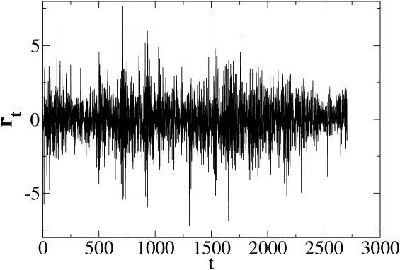
Figure 1: Time series of returns of the Nikkei 225 index.

The adaptive construction scheme is implemented as follows. First we make a short run by an MCMC method. Any MCMC method can be used. Here we use the Metropolis algorithm. We discard the first 5000 data as burn-in process (thermalization). Then we accumulate 1000 data to estimate $M$ and $\Sigma$. The estimated $M$ and $\Sigma$ are substituted to $g(\theta)$ of eq.(15). The shape parameter $\nu$ is set to 10. We re-start a run by the MH algorithm with the proposal density $g(\theta)$. Every 1000 update we re-calculate $M$ and $\Sigma$ using all accumulated data and update $g(\theta)$ for the next run. We accumulate 100000 data for analysis. The results analyed are summarized in Table 1.

We examine the efficiency of the algorithm by measuring correlations between sampled data. Fig.2 shows the autocorrelation function (ACF) of the sampled $\alpha$ with the Nikkei 225 index data. The ACF is defined as

$$ACF(t)=\frac{\frac{1}{N}\sum_{j=1}^{N}(x(j)-\langle x\rangle)(x(j+t)-\langle x\rangle)}{\sigma^{2}_{x}},$$ (20)

where $\langle x\rangle$ and $\sigma^{2}_{x}$ are the average value and the variance of certain successive data $x$ respectively. The ACF quickly decreases with $t$, which indicates that the correlation between the sampled data is very small. We also find the similar behavior for the other parameters.

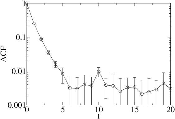
Figure 2: Autocorrelation functions of $\alpha$ sampled with the Nikkei 225 index data.

In order to analyze the autocorrelation quantitatively we measure the integrated autocorrelation time $\tau_{int}$ given by

$$\tau_{int}=\frac{1}{2}+\sum_{i=1}^{\infty}ACF(i).$$ (21)

”$2\tau_{int}$” is also called inefficiency factor. If no correlation exists in the data $2\tau_{int}$ takes one. The results of $2\tau_{int}$ are summarized in Table 1. We find that all the $2\tau_{int}$ are very small, less than 2, which indicates that the correlation between the data sampled by this method is small.

Table 1: Results of QGARCH parameters. SD and SE stand for standard deviation and statistical error respectively. Theoretically there is a relation of $SE\approx\sqrt{\frac{2\tau_{int}}{N}}SD$. Here statistical errors are estimated by the jackknife method.

	$\alpha$	$\beta$	$\omega$	$\gamma$
Nikkei 225	0.07872	0.89390	0.06219	-0.12403
SD	0.011	0.013	0.013	0.021
SE	0.00003	0.00004	0.00005	0.00007
$2\tau_{int}$	$2.0\pm 0.1$	$2.0\pm 0.1$	$2.0\pm 0.2$	$1.8\pm 0.1$
DAX	0.09198	0.89564	0.03004	-0.08483
SD	0.011	0.011	0.0064	0.015
SE	0.00004	0.00005	0.00004	0.00006
$2\tau_{int}$	$1.77\pm 0.06$	$1.78\pm 0.05$	$1.80\pm 0.07$	$1.61\pm 0.06$
Hang Seng	0.07638	0.91168	0.03202	-0.08678
SD	0.009	0.0098	0.007	0.007
SE	0.00005	0.00005	0.00003	0.00007
$2\tau_{int}$	$1.80\pm 0.06$	$1.78\pm 0.06$	$1.79\pm 0.06$	$1.75\pm 0.06$

Fig.3 and 4 show the convergence property of the covariance matrix. Here $V$ is a $4\times 4$ matrix defined by $V=E[(\theta-M)(\theta-M)^{t}]$. The elements $V_{11}$ and $V_{12}$ quickly converge to certain values. We also see the similar behavior for the other elements.

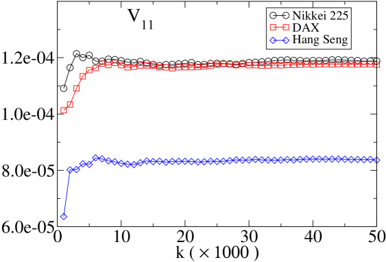
Figure 3: The diagonal element $V_{11}$ as a function of Monte Carlo time.

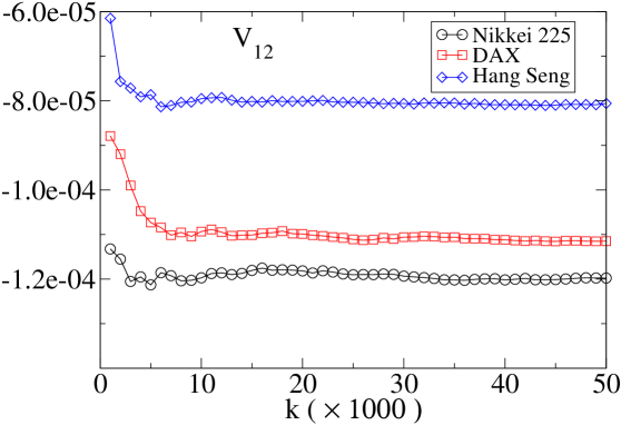
Figure 4: The off-diagonal element $V_{12}$ as a function of Monte Carlo time.

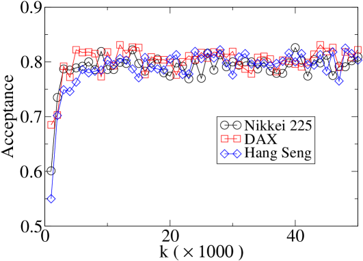
Figure 5: Acceptance at the MH algorithm with the adaptive proposal density.

Fig.5 shows the acceptance at the MH algorithm with the adaptive proposal density of eq.(15). Each acceptance is calculated every 1000 updates and the calculation of the acceptance is based on the latest 1000 data. At the first stage of the simulation the acceptance is low. This is because $M$ and $\Sigma$ have not yet been calculated accurately at this stage as seen in figs. 3-4. The acceptance increases quickly as the simulation is proceeded and reaches plateaus of about $80\%$.

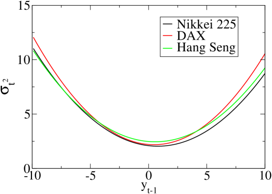
Figure 6: News impact curves of the Nikkei 225, DAX and Hang Seng indexes.

The QGARCH model is capable of capturing leverage effects. In order to see the impact of leverage effects Pagan and Schwert[25], and Engle and Ng[26] proposed the use of the so-called news impact curve. The news impact curve is the functional relationship between conditional variance at time $t$ and the shock at time $t-1$, $y_{t-1}$.

The news impact curve of the QGARCH model is given by

$$\sigma_{t}^{2}=\omega+\gamma y_{t-1}+\alpha y_{t-1}^{2}+\beta\sigma^{2},$$ (22)

where $\sigma^{2}$ is the unconditional variance given by

$$\sigma^{2}=\frac{\omega}{1-\alpha-\beta}.$$ (23)

Fig.6 shows the impact curves of Nikkei 225, DAX and Hang Seng indexes. Since the values of $\gamma$ for three indexes are all negative the three indexes exhibit the leverage effect. As seen in fig.6 the news impact curve is higher for negative $y_{t-1}$ than for positive one. Since all the three news impact curves are very similar each other the three indexes turn out to have the similar responce to positive or negative news.

8 Conclusions

We have performed the Bayesian inference of the QGARCH model by the MCMC algorithm. The MCMC algorithm was implemented by the MH method with the adaptive proposal density. The adaptive proposal density is assumed to be the Student’s t-distribution and the distribution parameters are determined by the data sampled by the MCMC simulation. The distribution parameters are updated during the MCMC simulation adaptively to match the posterior density of the model parameters.

We have applied our method for Nikkei 225, DAX and Hang Seng indexes. We find that the autocorrelation times between the sampled data are very small, typically $2\tau_{int}$ is less than 2. Thus our method is very efficient for generating uncorrelated Monte Carlo data.

The QGARCH model is designed to capture the leverage effect. We find that all the three indexes show the leverage effect, i.e. the volatility is higher after negative observations than after positive ones.

The acceptance of the MH algorithm quickly reaches a plateau of about 80% already at the beginning of the simulation. This means that the distribution parameters are evaluated accurately already at the beginning of the simulation, as shown in figs.3-4. This observation suggests that in practice one may stop the update of the parameters at some stage of the simulation.

References

References

- [1] Engle R F 1982 Autoregressive Conditional Heteroskedasticity with Estimates of the Variance of the United Kingdom inflation Econometrica 60 987
- [2] Bollerslev T 1986 Generalized Autoregressive Conditional Heteroskedasticity Journal of Econometrics 31, 307–327 (1986)
- [3] Duarte Queiros S M and Tsallis C 2005 Bridging the ARCH model for finance and nonextensive entropy Europhys. Lett. 69 893
- [4] Duarte Queiros S M and Tsallis C 2005 On the connection between financial processes with stochastic volatility and nonextensive statistical mechanics Eur. Phys. J. B 48 139
- [5] Black F 1976 Studies of Stock Market Volatility Changes 1976 Proceedings of the American Statistical Association, Business and Economic Statistics Section 177
- [6] Nelson D B 1991 Conditional Heteroskedasticity in Asset Returns: A New Approach Econometrica 59, 347
- [7] Glosten L R, Jaganathan R and Runkle D E 1993 On the Relation Between the Expected Value and the Volatility of the Nominal Excess on Stocks Journal of Finance 48 1779
- [8] Ding Z, Granger C W J and Engle R F 1993 A Long Memory Property of Stock Market Returns and a New Model Journal of Empirical Finance 1, 83
- [9] Zakoïan M 1994 Threshold Heteroscedastic Models Journal of Economic Dynamics and Control 18 931
- [10] Engle R F and Ng V 1993 Measuring and testing the impact of news on volatility Journal of Finance 48 1749
- [11] Sentana E 1995 Quadratic ARCH models Review of Economic Studies 62 639
- [12] Bauwens L and Lubrano M 1998 Bayesian inference on GARCH models using the Gibbs sampler Econometrics Journal 1 c23
- [13] Kim S Shephard N and Chib S 1998 Stochastic volatility: Likelihood inference and comparison with ARCH models Review of Economic Studies 65 361
- [14] Nakatsuma T 2000 Bayesian analysis of ARMA-GARCH models: Markov chain sampling approach Journal of Econometrics 95 57
- [15] Vrontos I D, Dellaportas P and Politis D N 2000 Full Bayesian inference for GARCH and EGARCH models Journal of Business and Economic Statistics 18 187
- [16] Mitsui H and Watanabe T 2003 Bayesian analysis of GARCH option pricing models J. Japan Statist. Soc. (Japanese Issue) 33 307
- [17] Asai M 2006 Comparison of MCMC Methods for Estimating GARCH Models J. Japan Statist. Soc. 36 199
-
[18]
Takaishi T 2006
Bayesian Estimation of GARCH model by Hybrid Monte Carlo
P͡roceedings of the 9th Joint Conference on Information Sciences 2006 CIEF-214
doi:10.2991/jcis.2006.159 - [19] Ardia D 2008 Financial Risk Management with Bayesian Estimation of GARCH models (Springer)
- [20] Takaishi T (2009) An Adaptive Markov Chain Monte Carlo Method for GARCH Model Preprint arXiv:0901.0992v1
-
[21]
Takaishi T 2009
Bayesian Estimation of GARCH Model with an Adaptive Proposal Density
New Advances in Intelligent Decision Technologies,
Studies in Computational Intelligence Volume 199 635
doi:10.1007/978-3-642-00909-9_61 -
[22]
Takaishi T 2009
Bayesian Inference on QGARCH Model Using the Adaptive Construction Scheme
Proceedings of 8th IEEE/ACIS International Conference on Computer and Information Science
525
doi:10.1109/ICIS.2009.173 - [23] Metropolis N et al. 1953 Equations of State Calculations by Fast Computing Machines J. of Chem. Phys. 21 1087
- [24] Hastings W K 1970 Monte Carlo Sampling Methods Using Markov Chains and Their Applications Biometrika 57 97
- [25] Pagan A and Schwert G W 1990 Alternative Models for Conditional Volatility Journal of Econometrics 45 267
- [26] Engle R F and Ng V 1993 Measuring and Testing the Impact of News on Volatility Journal of Finance 48 1749