Directional Radiation and Photodissociation Regions
in Molecular Hydrogen Clouds

Some astrophysical observations of molecular hydrogen point to a broadening of the velocity distribution for molecules at excited rotational levels. This effect is observed in both Galactic and high redshift clouds. Analysis of H₂, HD, and C I absorption lines has revealed the broadening effect in the absorption system of QSO 1232+082  ($z_{\rm abs}=2.33771$). We analyze line broadening mechanisms by considering in detail the transfer of ultraviolet radiation (in the resonance lines of the Lyman and Werner H₂ molecular bands) for various velocity distributions at excited rotational levels. The mechanism we suggest includes the saturation of the lines that populate excited rotational levels (radiative pumping) and manifests itself most clearly in the case of directional radiation in the medium. Based on the calculated structure of a molecular hydrogen cloud in rotational level populations, we have considered an additional mechanism that takes into account the presence of a photodissociation region. Note that disregarding the broadening effects we investigated can lead to a significant systematic error when the data are processed.

INTRODUCTION

Molecular hydrogen, the most abundant molecule in the interstellar medium, is observed not only in our Galaxy (Savage et al. (1977); Shull & Beckwith (1982); Rachford et al. (2002)) and Local Group galaxies (Tumlinson et al. (2002); Bluhm et al. (2003)) but also in the spectra of high-redshift quasars (see Levshakov & Varshalovich (1985); Noterdaeme et al. (2008)).

The importance of molecular hydrogen, particularly at the early evolutionary phases of the Universe, lies in the fact that it plays a key role in the theory of star formation, being the main coolant. Observations of various rotational H₂ states allow the main physical parameters (kinetic temperature, pressure, particle density, etc.) to be determined in the molecular hydrogen clouds that existed 12 Gyr ago. The relative population of rotational H₂ levels also makes it possible to estimate the intensity of ultraviolet radiation, whose high value can serve as an indicator of active star formation in early protogalaxies. In addition, precision measurements of molecular hydrogen wavelengths at high redshifts are used to estimate the possible cosmological change in the proton-to-electron mass ratio (see, e.g., Ivanchik et al. (2005)).

The ground X${}^{1}\Sigma_{g}^{+}$ and excited B${}^{1}\Sigma_{u}^{+}$ and C${}^{1}\Pi_{u}$ electronic states are distinguished in the molecular hydrogen level structure. There are vibrational and finer rotational level structures in each electronic state (see Fig. 1).

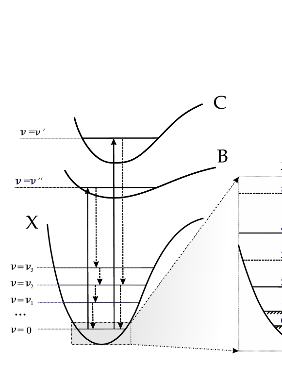
Figure 1: Level diagram for the hydrogen molecule. The ground X${}^{1}\Sigma_{g}^{+}$ and excited B${}^{1}\Sigma_{u}^{+}$ and C${}^{1}\Pi_{u}$ electronic states are presented. The vibrational structure of the electronic levels is shown. The rotational structure for the lower vibrational, ground electronic state, in which the times of spontaneous transitions are indicated, is presented on the right panel.

Since the dipole transitions are forbidden in the ground electronic state, molecular hydrogen is commonly observed using the system of lines between the ground X state and the excited B and C states, which are called the Lyman and Werner bands, respectively. These bands lie in the ultraviolet spectral range. However, for hydrogen at high redshifts (z$\,\,\sim\,\,2\div 4$), the absorption lines fall within the visible spectral range. Therefore, it can be observed using groundbased telescopes with a high spectral resolution.

Another peculiarity of the hydrogen molecule is the mechanism of its dissociation. The point is that the dissociation continuum of molecular hydrogen is higher than that of atomic one. This means that there is no direct photodissociation of molecular hydrogen in the interstellar medium, because atomic hydrogen depletes the spectrum above 13.6 eV. The dissociation proceeds through the mechanism that was first described by Stecher & Williams (1967). After their excitation in the Lyman or Werner bands, about 87 % of the molecules return rapidly, in a time $\tau\sim 10^{-6}\,\mbox{s}$, to the ground electronic state at upper ro-vibrational levels, while 13 % of the molecules fall into the continuum, i.e., dissociate (Abgrall et al. (1992)). The undissociated molecules fall into the lower vibrational state through cascade transitions and populate the long-lived rotational levels (see Dalgarno & Black (1974)). This mechanism is called radiative pumping.

The absence of dipole transitions in the lower vibrational, ground electronic state not only makes the rotational levels basically metastable but also strongly suppresses the direct radiative population. The typical physical conditions in molecular hydrogen clouds are $T\sim 50\div 150\,\mbox{K}$, $n\sim 10\div 1000\,\mbox{sm}^{-3}$ (Rachford et al. (2002), Shull et al. (2000)). At such parameters, the collision rate is too low (compared to the rates of spontaneous transitions) for the excited rotational levels to be populated. Therefore, being in background ultraviolet radiation with an intensity $I\sim 10^{-18}\,\mbox{erg/sm}^{2}\mbox{/s/Hz}$ (for our Galaxy, at wavelengths of the order of $\lambda=1000\,$Å, Draine (1978)), the excited rotational $J>2$ levels are populated mainly through radiative pumping.

Fourteen absorption systems of molecular hydrogen have been identified to date in the spectra of distant quasars (Noterdaeme et al. (2008), Srianand et al. (2008)). One of these belongs to the spectrum of QSO 1232+082. The peculiarity of this system is that the effective width parameter of the velocity distribution $b$ for the excited rotational levels of hydrogen molecules is larger than the parameter $b$ for HD molecules and C I atoms (Ivanchik et al., to be published). In this paper, we will show how the propagation of directional radiation can broaden the velocity distribution of H₂ molecules at the levels populated by radiative pumping. In addition to our effect, we will consider a model that takes into account the presence of a photodissociation region, as was suggested by Noterdaeme et al. (2007).

OBSERVATIONAL DATA

The Absorption System in the Spectrum QSO 1232+082

The absorption system in the spectrum of QSO 1232+082   has been known since 1999 (Ge & Bechtold (1999)). It was measured in more detail by Petitjean et al. (2000) with the 8.2-m VLT telescope using theUVES echelle spectrograph. Subsequently, in 2001, HD molecules were first detected in this system at high redshifts (Varshalovich et al. (2001)). This had long been the only identification of HD molecules at high redshifts (the second system was identified by Srianand et al. (2008)). Analysis of this system revealed evidence for a broadening of the velocity distribution of molecules at excited rotational levels of molecular hydrogen. This effect is important in that assigning the same Doppler parameter to all rotational levels leads to a systematic error in the column density and, as a result, in other physical parameters of the system.

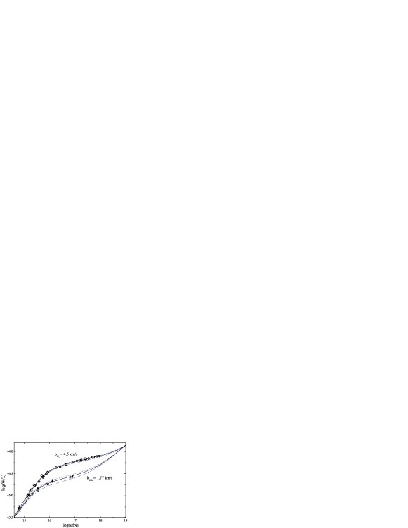
Figure 2: Standard curves of growth for the H₂, HD, and C I lines corresponding to the z = 2.33771 absorption system of QSO 1232+082. The equivalent widths for various excited rotational H₂ levels are plotted: $J=2$ (squares), $J=3$ (circles), $J=4$(diamonds), and $J=5$(asterisks). The equivalent widths of the transitions from the excited rotational levels fall best on the standard curve of growth with $b=4.5\,\mbox{km/s}$. Also shown are the HD (upward triangles) and CI (downward triangles) data. The standard curves of growth with $b=1.77\,\mbox{km/s}$ $b=1.67\,\mbox{km/s}$ are presented for HD and C I, respectively.

The data on the absorption system of QSO 1232+082   used here are presented in Fig. 2. We used the curve-of-growth method to analyze the data. The curve of growth shows the dependence of the line equivalent width on the column density. Since it also depends on the transition line parameters, the column density of an element and the distribution parameters can be determined in certain cases given the set of various lines. For a Maxwellian distribution (with the Doppler parameter $b$), the curve of growth is said to be a standard one. In our paper, we use a nonequilibrium velocity distribution to construct the curve of growth and call this curve a nonstandard one. Figure 2 shows the equivalent widths for various excited rotational levels of H₂ ($J=2,3,4,5$), HD, and C I. In addition, the standard curves of growth are plotted in the figure for $b=4.5\,\mbox{km/s}$ $b=1.77\,\mbox{km/s}$. The equivalent widths for the HD lines (upward triangles) fall best on the curve of growth with $b=1.77\,\mbox{km/s}$. The data on carbon (downward triangles) for this cloud have the Doppler parameter $b=1.67\,\mbox{km/s}$. It thus follows that the equivalent widths of the H₂ lines should have had $b$ equal to $b=1.82\,\mbox{km/s}$. However, the excited rotational levels of molecular hydrogen fall best on the curve of growth with $b=4.5\,\mbox{km/s}$, i.e., they have a distribution that is two and a half times broader than that expected from our analysis of the HD and C I data. Note that the Doppler parameter $b$ for the $J=0,1$ rotational levels cannot be determined by the curve-of-growth method, because the absorption lines are strongly saturated and their equivalent widths fall on the square-root segment where the curves of growth with various $b$ merge together. Thus, a broadening of the velocity distribution at excited rotational levels of molecular hydrogen manifests itself in this system.

Observations of the Broadening Effect in Other Systems

A broadening of the effective Doppler parameter $b$ with increasing rotational level $J$ was observed previously for our Galaxy (Spitzer & Cochran (1973), Jenkins & Peimbert (1997), Lacour et al. (2005)) and in a high-redshift system Noterdaeme et al. (2007)). Spitzer & Cochran (1973) were the first to notice this effect while analyzing the curve of growth for observations with the ultraviolet telescope of the Copernicus Orbital Observatory. However, since the data had large errors, it is hard to say whether this effect is systematic. Much later, the observations by Jenkins & Peimbert (1997) on IMAPS revealed a broadening in molecular hydrogen toward $\zeta\,$ Ori A. Several years ago, while observing excited rotational levels of molecular hydrogen in the directions of four young stars from the FUSE satellite, Lacour et al. (2005) found that such an effect was present in all four directions. The fourth and most recent observation refers to extragalactic molecular hydrogen. Noterdaeme et al. (2007) revealed this effect for the absorption system at redshift $z=2.402$ in the spectrum of the quasar HE 0027 -1836.

Note that no satisfactory explanation for the broadening effect has existed until now. Different authors use different models to explain it. The system observed by Jenkins & Peimbert (1997) is peculiar in that the line profiles exhibit three components for which the column densities at rotational levels are low ($N_{J}\lesssim 10^{15}\,\mbox{sm}^{-2}$ and that there exists a systematic shift in the velocities with increasing rotational level. This enables the authors to explain the effect in question by a model with a shock. The observed broadening and the velocity shifts stem from the fact that the flow from the shock front gradually cools down and decelerates. This model runs into difficulties in explaining the data in which one component of molecular hydrogen is observed, there are no velocity shifts for various rotational levels, and the H₂ column densities are high.

Lacour et al. (2005) assume that during its formation on dust, the hydrogen molecule acquires an additional energy of $\sim 4.5\,\mbox{eV}$ that is distributed between the vibrational, rotational, and translational degrees of freedom. In other words, the molecules are formed in excited states with an excess kinetic energy. However, the authors point out that the formation rate of molecules on dust should be an order of magnitude higher to explain the broadening effect. This is particularly problematic for the high-redshift absorption systems of molecular hydrogen associated with damped Ly-$\alpha$ systems; observations of the metallicity in the latter (Ledoux et al. (2003), Noterdaeme et al. (2008)) show that the dust content in them is more than an order of magnitude lower than that in our Galaxy. The damped Ly-$\alpha$ systems are the systems with very high atomic hydrogen column densities (N(H I) $>10^{20}\,\mbox{sm}^{-2}$) that are observed in quasar spectra and that are probably high-redshift protogalaxies.

Another explanation for the broadening effect was also offered by Noterdaeme et al. (2007). They showed that the broadening could be explained by the presence of two components in the cloud. The first component is under the influence of strong background ultraviolet radiation, which increases the radiative pumping of excited rotational levels and heats up the medium through hydrogen dissociation this is the so-called photodissociation region (Hollenbach & Tielens (1999)). In the second component, the ultraviolet radiation is appreciably weaker; therefore, it is colder and the excited levels are populated sparsely. In that case, the excited and ground rotational levels manifest themselves mainly in the hot and cold components, respectively, which can provide the observed effect. As will be shown below, when the radiative transfer in the Lyman and Werner bands is considered, these regions naturally emerge in the same molecular cloud.

Note that Lacour et al. (2005), Noterdaeme et al. (2007) assumed that radiative pumping could not produce a broadening. The authors placed emphasis on the fact that the molecule did not change its velocity during radiative pumping transitions and sought for other possible explanations. This assertion is beyond doubt. However, we will show in the next section that when the transfer of directional radiation is considered in detail, a broadening at the levels being populated can arise during radiative pumping if the population from the line wings is taken into account.

MAIN POINTS OF THE MODEL

A broadening of the velocity distribution at the levels populated by radiative pumping can be obtained by considering the radiative transfer. The broadening effect will be at a maximum during the propagation of directional radiation. Therefore, let us consider a molecular hydrogen cloud on which directional radiation with an intensity $I(\nu,z)$ falls (see Fig. 3). We will be interested in the velocity distribution of the molecules populated by radiative pumping as a function of the depth of radiation penetration into the cloud.

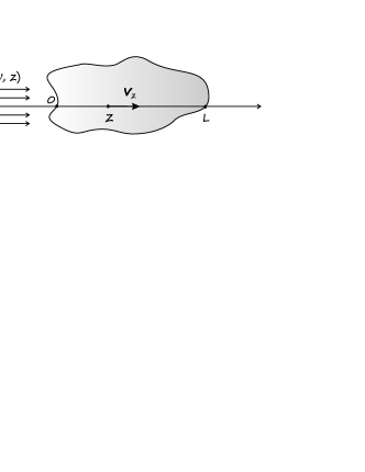
Figure 3: Geometric model of cloud. Directional radiation with an intensity $I(\nu,z)$ falls on the cloud.

To understand the effect qualitatively, let us consider a three-level system (see Fig. 4). Naturally, this system will fully reflect the main physical properties of the hydrogen molecule of interest to us and it can be used as an example to obtain the broadening effect analytically. Thus, we have the ground level ($0$) that acts as a reservoir. A metastable level $l$ is radiatively pumped from the ground level through the system s photoexcitations to level $k$ followed by its relaxation to level $l$. The direct transitions from the ground level to level $l$ will be assumed to be forbidden.

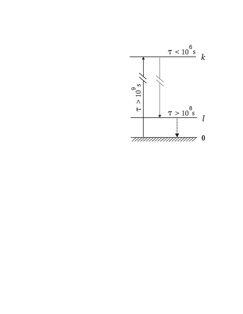
Figure 4: Three-level system: $0$ is the ground level from which level $l$ is radiatively pumped through the resonance level $k$. The characteristic time scales of the processes considered in this system corresponding to a hydrogen molecule in the interstellar medium are shown near the arrows indicating these processes.

Based on the characteristic time scales shown in Fig. 4 (which correspond to those for the hydrogen molecule), we can assume that the system passes from level $k$ to level $l$ almost instantly. Since level $l$ is metastable, we can observe the molecules at this level. To obtain the velocity distribution of the molecules at level $l$, let us consider the balance equation for the molecules at the level

$$n_{l}(v_{z},z)A_{l}=n_{0}(v_{z},z)P_{0k}(v_{z},z)$$ (1)

The left-hand and right-hand sides of the equation describe, respectively, the spontaneous downward transitions and the population of level $l$ from the ground level through radiative pumping via level $k$. $P_{0k}$ is the capability of the particles to pass to level $k$ under radiation or the fraction of the particles that pass to level $k$ per unit time at depth $z$ and that have a velocity $v_{z}$; in other words, $P_{0k}$ is the photoexcitation rate:

$$P_{0k}(v_{z},z)=\int\limits_{-\infty}^{+\infty}\frac{I(\nu,z)}{h\nu}\kappa_{0k}\left(\nu+\nu\frac{v_{z}}{c}\right)d\nu.$$ (2)

It is important to note that this quantity is a function of $(v_{z},z)$.

We can neglect the multiple scatterings while considering the radiative transfer in the cloud, since the resonance photons that accomplish radiative pumping fragment as the excited states decay due to the presence of a ro-vibrational cascade in the H₂ molecule. Therefore, we can use a radiative transfer equation in the form

$$I(\nu,z)=I(\nu,0)e^{-\tau_{0k}(\nu,z)},$$ (3)

where

$$\tau_{0k}(\nu,z)=\int\limits_{0}^{z}dz^{\prime}\int\limits_{-\infty}^{+\infty}dv_{z}n_{0}(v_{z},z^{\prime})\kappa_{0k}\left(\nu+\nu\frac{v_{z}}{c}\right).$$ (4)

The quantity $\kappa_{0k}$ in Eqs. (2) and (4) is the photoexcitation cross section for the $0\to k$ transition.

The Broadening Effect

An expression for the velocity distribution of the molecules at level $l$ can be obtained by rewriting Eq. (1) using Eq. (2):

$$n_{l}(v_{z},z)=\frac{n_{0}(v_{z},z)}{A_{l}}\int\limits_{-\infty}^{+\infty}\frac{I(\nu,z)}{h\nu}\kappa_{0k}\left(\nu+\nu\frac{v_{z}}{c}\right)d\nu.$$ (5)

The distribution at level $l$ is broadened during the formation of an absorption line in the $0\to k$ transition followed by the population of level $l$ (Fig. 4). Figure 5 presents the calculated number and column densities and line profiles for typical molecular hydrogen line parameters (we chose the L3-0R(0) line). In what follows, we assume that the distribution at the ground level $0$ is Maxwellian.

Figure 5: Spectral resonance line profiles and velocity distributions of molecules. The calculation is presented for three optical depths at the line center: (a) $\tau_{0}=0.2$, (b) $\tau_{0}=20$, and (c) $\tau_{0}=1000$. The upper panels show the profile of the line through which level $l$ is radiatively populated. The middle panels show the normalized molecular number density distribution produced by radiative pumping. The lower panels show the normalized molecular column density distribution integrated along the line of sight to the depth corresponding to the line profile on the upper panels.

The upper panels in Fig. 5 (a1, b1, c1) present the line profile for a given optical depth $\tau_{0}$ at the line center (indicated above the panels). The middle panels (a2, b2, c2) show the normalized distribution of the number density populated by radiative pumping to level $l$ at depth $z$ where the line profile was formed. The presented number density distributions were normalized to the area under the distribution for $\tau_{0}=0.2$ (panel (a2)). Therefore, the area under the distributions for $\tau_{0}=20$ (panel (b2)) and $\tau_{0}=1000$ (panel (c2)) shows the extent to which the total photoexcitation rate decreases compared to the depth where $\tau_{0}=0.2$. The lower panels (a3, b3, c3) display the normalized distribution of the column density, i.e., integrated over the line of sight to depth $z$. The column density distributions were normalized to the area of the distribution under its curve for $\tau_{0}=1000$ (panel (c3)). The velocity in km/s is along the $x$ axes (for the line profile, this corresponds to the Doppler wavelength shift). We see that as long as the line profile is unsaturated ($\tau_{0}=0.2$, (a1)), the populated (a2) and column (a3) densities correspond to a Maxwellian distribution at the ground level, i.e., no broadening occurs. When the lines are saturated ($\tau_{0}=20$, (b1)), the distribution populated to level $l$ becomes a highly nonequilibrium one. As long as the absorption is a Doppler one, the molecule absorbs a photon that closely corresponds to its Doppler velocity shift. In other words, the photoexcitation cross section $\kappa_{ok}$ in Eq. (5) can be replaced with a delta function; therefore, the dependence of the photoexcitation cross section $P_{0k}$ on the velocity of the molecule will closely correspond to the profile of the $0\to k$ transition line. When the line is saturated, the photons are deficient at the line center and the population takes place mainly at the line edges, where the photons are plenty. Therefore, the number density distribution at level $l$ becomes a highly nonequilibrium one (panel (b2)). The column density distribution (panel (b3)) is an observable quantity in the spectra; it exhibits a broadening with the formation of a plateau.

As the line is saturated further ($\tau_{0}=1000$, (c1)), i.e., as the radiation penetrates deeper into the medium, the Lorentz wings will manifest themselves in the line profile. This means that level $l$ will also be populated in the Lorentz wings. In this case, the transition wavelength does not corresponds to the Doppler velocity shift and the replacement of $\kappa_{0k}$ with a delta function is invalid. This population is peculiar in that the distribution populated by the Lorentz wings will correspond to the distribution at the ground level, i.e., it will be Gaussian. We see from panel (c2) that even a small fraction at a given optical depth corresponds to a nonequilibrium distribution. Thus, the population in the Lorentz wings can greatly reduce the broadening of the column density distribution (panel (c3)).

The nonequilibrium distribution populated to level $l$ will manifest itself in the absorption lines from this level, while the lines will not be described by a Voigt profile. When a Voigt profile is fitted into the line, the effective width parameter of the Maxwellian distribution $b$ will naturally be larger than that for the ground level. Therefore, when we analyze the absorption lines for level $l$ and use the standard theory of radiative transfer, the parameter $b$ to be determined will effectively increase.

Thermalization and Turbulence

The nonequilibrium distribution populated to level $l$ can be thermalized with time or remain broadened in the presence of turbulent motions. It all depends on the relationships between the rates of characteristic processes. To describe the turbulent motions, we will use the assumption about microturbulence under which the distribution in the cloud in turbulent velocity $w_{turb}$ is described by a Gaussian function with a parameter $b_{turb}$. The ground level may be considered to be thermalized, i.e., the velocity distribution of the molecules related to thermal motion, $w_{th}$, is described by a Maxwellian distribution with a parameter $b_{th}$. The total distribution obtained by a convolution of the turbulent and thermal distributions will then be Maxwellian with the parameter $b=\sqrt{b^{2}_{turb}+b^{2}_{th}}$ Therefore, the relationship between the following three rates of the processes should be considered: the thermalization rate, the turbulization rate, and the photoexcitation rate from level $l$. The turbulization rate may be considered to be much lower than the other two rates. If the thermalization rate is higher than the photoexcitation rate from level $l$, then the distribution that manifests itself in the absorption line from level $l$ will be thermalized.

The distribution thermalization effect for static turbulence can be written as

$$\tilde{n}_{l}(v_{z},z)=\int\limits_{-\infty}^{+\infty}dv^{\prime}_{z}\,n_{l}(v^{\prime}_{z},z)w_{+}\left(v_{z}-v^{\prime}_{z}\frac{b^{2}_{turb}}{b^{2}}\right).$$ (6)

(for the derivation, see the Appendix).

When $b_{th}\to 0$   $w_{+}(v)\to\delta(v)$ and, hence, $\tilde{n}_{l}(v,z)\equiv n_{l}(v,z)$, i.e., the nonequilibrium distribution is retained. When $b_{turb}\to 0$, $w_{+}$ does not depend on $v_{z}$ and the velocity distribution is completely thermalized, acquiring a Gaussian shape with $b=b_{th}$.

Optical Depths of Broadened Lines

As a result, we find that, given thermalization (6), the distribution at level $l$ will be

$$\tilde{n}_{l}(v_{z},z)=\frac{n_{0}(z)}{A_{l}}\int\limits_{-\infty}^{+\infty}dv^{\prime}_{z}\,P_{0k}(v^{\prime}_{z},z)\times\\ \times n_{0}(v^{\prime}_{z},z)w_{+}\left(v_{z}-v^{\prime}_{z}\frac{b^{2}_{turb}}{b^{2}}\right).$$ (7)

As we showed above, the particle velocity distribution at level $l$ (5) can manifest itself in the absorption line associated with the transition from this level to some resonance level $m$. We will assume that the absorption line profile is defined by the optical depth in accordance with Eq. (3). The optical depth $\tau_{lm}\,$ for the $l\to m\quad$ transition will have the form (4) with the cross section $\kappa_{lm}$ corresponding to the transition and the number density $\tilde{n}_{l}(v_{z},z)$ given in (6). Thus, we obtain

$$\tau_{lm}(\nu,L)=\int\limits_{0}^{L}dz\int\limits_{-\infty}^{+\infty}dv_{z}\kappa_{lm}\left(\nu+\nu\frac{v_{z}}{c}\right)\tilde{n}_{l}(v_{z},z)=\\ =\int\limits_{0}^{L}dz\int\limits_{-\infty}^{+\infty}dv_{z}\kappa_{lm}\left(\nu+\nu\frac{v_{z}}{c}\right)\times\\ \times\int\limits_{-\infty}^{+\infty}dv^{\prime}_{z}n_{l}(v^{\prime}_{z},z)w_{+}\left(v_{z}-v^{\prime}_{z}\frac{b^{2}_{turb}}{b^{2}}\right).$$ (8)

It is important to note that in our approximations, the $z$ dependence is present only in $n_{l}(v_{z},z)$. Using Eq. (5), we can represent the expression for the optical depth as

$$\tau_{lm}(\nu)=\int\limits_{-\infty}^{+\infty}dv^{\prime}_{z}\,W_{l}(v^{\prime}_{z})\tau^{+}_{lm}\left(\nu+\nu_{lm}\frac{v^{\prime}_{z}}{c}\frac{b^{2}_{turb}}{b^{2}}\right),$$ (9)

where $W_{l}(v_{z})$ is the nonequilibrium distribution of the particles thrown to level $l$ integrated along the line of sight:

$$W_{l}(v_{z})=\frac{N_{l}(v_{z})}{\int\limits_{-\infty}^{+\infty}dv_{z}\,N_{l}(v_{z})}=\frac{\int\limits_{0}^{L}dz\,n_{l}(v_{z},z)}{\int\limits_{0}^{L}dz\int\limits_{-\infty}^{+\infty}dv_{z}\,n_{l}(v_{z},z)}.$$ (10)

The quantity $\tau^{+}_{lm}$ in Eq. (9) is the optical depth in the standard theory of radiative transfer, which can be written via the Voigt function as

$$\tau^{+}_{lm}\left(\nu+\nu_{lm}\frac{v^{\prime}_{z}}{c}\frac{b^{2}_{turb}}{b^{2}}\right)=\sqrt{\pi}\frac{e^{2}}{m_{e}c}\frac{4\pi N_{l}f_{lm}a_{lm}}{\gamma}H(a_{lm},x),$$ (11)

where

$$a_{lm}=\frac{\gamma c}{4\pi\nu_{lm}b_{th}\sqrt{1+(b_{turb}/b)^{2}}},$$

$$x=-\frac{c}{b_{th}\sqrt{1+(b_{turb}/b)^{2}}}\left(1+\frac{v^{\prime}_{z}}{c}\frac{b^{2}_{turb}}{b^{2}}-\frac{\nu_{lm}}{\nu}\right).$$

We can write expressions for $N_{l}(v^{\prime}_{z})$ the column density distribution of the particles that are populated to level $l$ and that have no time to be thermalized. Using Eq. (5), we will find that

$$N_{l}(v_{z})=\int\limits^{L}_{0}dz\,n_{l}(v_{z},z)=\frac{1}{A_{l}}\int\limits^{L}_{0}dz\,n_{0}(v_{z},z)P_{0k}(v_{z},z).$$ (12)

For a uniform and equilibrium distribution at the ground level and for the radiative transfer equation written for the $i\to k$ lines in form (3), we can easily obtain

$$N_{l}(v_{z})=\frac{N_{0}}{A_{l}}w(v_{z})\int\limits_{-\infty}^{+\infty}d\nu\,\frac{I_{0}(\nu)}{h\nu}\times\\ \times\frac{(1-e^{-\tau_{0k}(\nu,L)})}{\tau_{0k}(\nu,L)}\kappa_{0k}\left(\nu+\nu\frac{v_{z}}{c}\right),$$ (13)

where $I_{0}(\nu)=I(\nu,z=0)$.

Passing to the limit in Eq. (9) allows physically meaningful expressions to be derived for the extreme cases:

1. The absence of turbulence ($b_{turb}\ll b_{th}$).

   In this case, $b_{th}\approx b$. Then,

   $$\tau_{lm}(\nu)=\int\limits_{-\infty}^{+\infty}dv^{\prime}_{z}W_{l}(v^{\prime}_{z})\tau^{+}_{lm}\left(\nu\right)=\tau^{+}_{lm}(\nu),$$ (14)

   where $\tau^{+}_{lm}$ is the optical depth in the standard theory of radiative transfer with a thermal broadening $b=b_{th}$. Thus, in this case, the nonequilibrium distribution radiatively populated upward is completely thermalized to become an equilibrium one and gives a standard shape for the line profile.

2. Dominant turbulence ($b_{turb}\gg b_{th}$).

   In this case, $b_{turb}\approx b$ and then $\tau^{+}_{lm}\left(\nu+\nu_{lm}\frac{v_{z}}{c}\frac{b^{2}_{turb}}{b^{2}}\right)$ will correspond to the cross section $\kappa_{lm}\left(\nu+\nu\frac{v_{z}}{c}\right)$ to constant coefficients and the broadening effect related to radiative pumping will manifest itself in full:

   $$\tau_{lm}(\nu,L)=\int\limits_{-\infty}^{+\infty}dv_{z}\kappa_{lm}\left(\nu+\nu\frac{v_{z}}{c}\right)N_{l}(v_{z}).$$ (15)

Nonstandard Curves of Growth

Using the above formulas, we can demonstrate how the broadening effect will appear in curve of growth representation. In Fig. 6, the dashed lines indicate the standard curves of growth for distribution parameters $b$ from 1.8 to 3.8 km/s at steps of 0.5 km/s. In the same figure, the circles indicate the curves of growth for the broadening effect that we calculated based on the three-level model. The curves of growth correspond to the transitions from level $l$, i.e., to the particle velocity distribution at level $l$. Since, as was shown above, this distribution can differ from the Maxwellian one, the curves of growth will also differ from the standard ones. The figure shows two limits: with (open circles, see (6)) and without (filled circles) thermalization.

Figure 6: Nonstandard curves of growth. The circles indicate the curves of growth for the velocity distribution of the molecules broadened by radiative pumping: the filled and open circles indicate the results of our calculation, respectively, without and with thermalization of the velocity distribution at the level. The following distribution parameters were chosen: $b_{th}=0.8\,\mbox{km/s}$, $b_{turb}=1.6\,\mbox{km/s}$. The dashed lines represent the standard curves of growth with parameters $b$ from 1.8 to 3.8 km/s at steps of 0.5 km/s. In the absence of a broadening effect, the nonstandard curves of growth marked by the circles would coincide with the lower standard curve of growth with $b=1.8\,\mbox{km/s}$.

The shape of the nonstandard curve of growth depends on certain parameters of the calculation. First, these include the parameter $b$, the width of the Maxwellian distribution at the ground level from which the population occurs. For the calculation in question, btot is $b_{tot}$ km/s, which corresponds to the lower standard curve of growth in Fig. 6 and agrees with the HD and C I data. For a thermalized distribution at level $l$ (open circles), the relationship between $b_{th}$ $b_{turb}$ should be specified. The broadening effect will depend on this relationship. Irrespective of the relationship between the characteristic time scales, the case without thermalization (filled circles) can take place for $b_{turb}\gg b_{th}$. In this case, the curve of growth passes higher, i.e., it corresponds to larger effective $b$ for the standard curves of growth. Naturally, the limit $b_{turb}\ll b_{th}$ corresponds to complete thermalization, with the nonstandard curve of growth coinciding with the standard one for $b=1.8\,\mbox{km/s}$. Second, the shape of the curve of growth depends on the column density at the ground level. This is easy to explain, since the shape of the distribution (Fig. 5, panels (c)) depends on the column density at the ground level in the cloud via the line profiles (Fig. 5, panels (a)). In the case under consideration, the column density was chosen to be $N_{0}=10^{19}\,\mbox{cm}^{-2}$.

It should be noted that the broadening effect manifests itself only in a certain range of column densities at the ground level. The distribution is not yet broadened at low column densities ($N_{tot}<10^{15}\,\mbox{cm}^{-2}$ for typical line parameters of the Lyman or Werner molecular hydrogen band). At high column densities ($N_{tot}>10^{20}\,\mbox{cm}^{-2}$), the broadening effect is suppressed by the Lorentz wings (see Fig. 5).

Thus, the inferred effective broadening takes place in the case of directional radiation in the cloud and using the standard curve of growth can lead to a systematic error in the column densities and distribution parameters.

A SCHEME FOR CALCULATING A MOLECULAR HYDROGEN CLOUD

Let us apply the broadening effect that we obtained in the previous section to molecular hydrogen. This effect arises when considering the transfer of directional radiation in a medium and is related to the peculiarity of the radiation interaction with the energy level structure. Therefore, we will consider a cloud composed only of molecular hydrogen. Since the radiation directionality is important for the manifestation of the broadening effect, we will consider a one-dimensional cloud model, i.e., one direction in which the radiation propagates coincident with our line of sight. In this approximation, we neglect the background radiation compared to the directional one, which is quite valid when a bright (in the ultraviolet) star (or a quasar) is close to the cloud. Naturally, in this case, the star lies behind the cloud and the line of sight coincides with the direction of the star. It is important to note that in this cloud model, we do not consider such processes and the photodissociation of molecular hydrogen and its formation on dust (Hollenbach et al. (1971), Jura 1975 ). A remark about the influence of dust will be made below.

Multilevel Model

When we pass from the three-level system to the real multilevel model of the hydrogen molecule, a number of peculiarities arise that should be taken into account.

The first important peculiarity is that there exist two different states of molecular hydrogen – ortho- and parahydrogen. In general, the direct radiative transitions between these states are forbidden ($\tau\sim 5\times 10^{12}$ yr). A much faster mixing of the ortho- and para-states is possible through collisions with $H^{+}$ and $H_{3}^{+}$ (Abgrall et al. (1992)) and during the dissociation of hydrogen followed by its formation. However, under our model assumptions, the ortho- and parahydrogen systems may be considered separately.

The second peculiarity consists in an allowance for the presence of many lines in the Lyman and Werner bands through which radiative pumping proceeds. This means that the sum over all the possible transitions of the Lyman and Werner bands will now appear in Eq. (2) for the photoexcitation rate. To calculate the latter, we used the wavelengths and oscillator strengths for the Lyman and Werner band transitions from Abgrall et al. 1993a , Abgrall et al. 1993b , respectively. The weight factor that describes the ro-vibrational cascade in the ground electronic state (Dalgarno & Black (1974)) should also be added. The ro-vibrational cascade is peculiar in that it allows high-lying rotational levels to be populated from low-lying ones (Jura 1975 ). We will assume that the ro-vibrational cascade occurs almost instantly, i.e., on time scales much shorter than those of the processes considered in our model.

The next remark is that the first several rotational levels of the hydrogen molecule should be considered jointly, i.e., we should depart from the consideration of the ground level as a reservoir. For example, the levels only with even rotational numbers ($J=0,2,4,$   etc.) are present in the parahydrogen system in the ground electronic state. Assuming that almost all of the molecules are at the lower vibrational level, we should take into account the radiative pumping of the $J=2$ level from the $J=0$ level and vice versa. We can restrict our analysis to the first several rotational levels, since the time scales of the spontaneous $J\to J-2$ transitions in the lower vibrational state decrease with increasing $J$; this means that the upper rotational levels can be included in the ro-vibrational cascade. The data for the ro-vibrational cascade that we used from Dalgarno & Black (1974) are restricted to the first eleven rotational levels, which are enough under typical conditions of the interstellar medium.

Yet another peculiarity is that although we disregarded the presence of atomic hydrogen, it can be assumed that there is a dip in the spectrum for $\lambda<912$ Å  related to the absorption of atomic hydrogen in the ionization continuum for the radiation incident on the cloud. This allows us to restrict our analysis of the transitions in the Lyman and Werner bands to the 20th and 6th vibrational levels, respectively. As a result, we calculated the radiative transfer for approximately 600 resonance lines of the Lyman and Werner H₂ bands.

Balance Equations

Let us write the balance equations for the system of molecular hydrogen levels under our assumptions. In a stationary situation,

$$\frac{\partial n_{i}(v_{z},z)}{\partial t}=0$$

and it is convenient to write the system of equations to determine the particle distributions at the levels in matrix form,

$$G(v_{z},z)n(v_{z},z)=0,$$ (16)

where $n(v_{z},z)$ is the column of the particle velocity distributions for various rotational levels; $G$ is the matrix that describes the transitions between the levels,

$$G(v_{z},z)=B(v_{z},z)+A+C,$$ (17)

where the matrix $A$ is related to spontaneous quadrupole transitions between rotational states, the matrix $C$ is related to collisional transitions, and the matrix $B$ is related to radiative pumping. The specific form of the matrix can be easily obtained by considering the balance between the particles going from and coming to some level $i$. For example, the components of the matrix $B$ can be represented as

$$B_{ij}=\Pi_{ij}-\delta_{ij}\sum\limits_{k}\Pi_{ik},$$ (18)

where $\delta_{ij}$ is the Kronecker symbol and $\Pi_{ij}$ is the photoexcitation rate for the transition from the $i$th rotational level to the $j$th one and, what is important, is a function of $(v_{z},z)$ and depends on $n_{i}(v_{z},z)$. This is related to radiative transfer, which manifests itself in the saturation of the radiative pumping line, and it is this fact that provides the required broadening. The photoexcitation rates can be written as

$$\Pi_{ij}=\sum\limits_{k}P_{ik}(v_{z},z)K_{kj},$$ (19)

where $k$ is the set (B(C), $\nu^{\prime},J^{\prime})$ ($J^{\prime}$ are the permitted rotational levels). Accordingly, $P_{ik}$ is the photoexcitation rate for the $i\to k$ transition:

$$P_{ik}(v_{z},z)=\int\limits_{-\infty}^{+\infty}\frac{I(\nu,z)}{h\nu}\kappa_{ik}\left(\nu+\nu\frac{v_{z}}{c}\right)\,d\nu,$$

and $K_{kj}$ is the probability to relax $k=$(B(C), $\nu^{\prime},J^{\prime})\to($X, $\nu=0,J=i)$; for convenience, it can be separated into the relaxation from excited electronic levels and the ro-vibrational cascade,

$$K_{kj}=\sum\limits_{\nu}\sum\limits_{J}G_{k(\nu,J)}\beta_{(\nu,J)i}\,,$$ (20)

where $G$ describes the relaxation from upper levels and $\beta$ is responsible for the cascade in the lower electronic state. We used the coefficients of the rovibrational cascade from Dalgarno & Black (1974). The collisional transition rates (matrix $C$) were taken from Abgrall et al. (1992).

System (16) is underdetermined, since one of the equations is not linearly independent. Therefore, we should exclude it and expand the system by an additional natural condition the condition on the total number density. Since, as we noted above, the ortho- and parahydrogen systems may be considered independently, the conditions on their total number density can be written separately:

$$n_{0}(v_{z},z)+n_{2}(v_{z},z)+s+n_{10}(v_{z},z)=n_{para}(v_{z},z),$$ (21)

for parahydrogen and a similar condition for orthohydrogen (with the total number density $n_{ortho}$): $n_{para}(v_{z},z)$ and $n_{ortho}(v_{z},z)$ are model-dependent quantities. We performed the calculation by assuming that these distributions were Maxwellian and that the integral of $n_{para}(v_{z},z)+n_{ortho}(v_{z},z)$ over all velocities was equal to the total number density of molecular hydrogen. Assuming that these systems are in thermodynamic equilibrium, the ratio of the para- and orthohydrogen number densities is determined by the temperature in the cloud (typically, $T\approx 100^{o}$ K).

System (16) should be solved numerically. We consider a homogeneous medium with typical molecular hydrogen number densities, $n_{\rm H_{2}}=10\div 1000\,\mbox{ }^{-3}$. $N_{tot}(z)$, the column density of molecular hydrogen to depth $z$, can serve as a measure of the depth of penetration into the cloud.

RESULTS

Main Results

The results of our calculations based on the scheme presented in the previous section are shown in Fig. 7 for various combinations of $N_{tot}$ (the total molecular hydrogen column density in the cloud) and $I_{0}$ (the intensity of the incident directional radiation). For two column densities $N_{tot}$, $10^{18}\,\mbox{cm}^{-2}$ $10^{19}\,\mbox{cm}^{-2}$, we chose three different intensities of the incident radiation: $10^{-16}$, $10^{-17}$ $10^{-18}$ $\mbox{erg/cm}^{2}\mbox{/s/Hz}$. Thus, there are a total of six different calculations (Fig. 7). The background isotropic radiation was assumed to be negligible compared to the directional one (this is valid when the directional radiation is determined by a nearby star or a quasar). For all calculations, the distribution parameters were chosen from observational data on HD and C I in the QSO 1232+082   absorption system: $b_{th}=0.81\,\mbox{km/s}$ for the thermal distribution and $b_{turb}=1.6\,\mbox{km/s}$ for the turbulent one; as a result, the Doppler parameter $b$ for the distributions $n_{para}(v_{z})$ and $n_{orto}(v_{z})$ (see (21)) is $b=\sqrt{b_{th}^{2}+b_{turb}^{2}}=1.8\,\mbox{km/s}$. The total molecular hydrogen number density was assumed to be uniform and the calculation was performed for several values of $n_{0}=n_{para}+n_{orto}=10,100,1000\,\,\mbox{cm}^{-3}$.

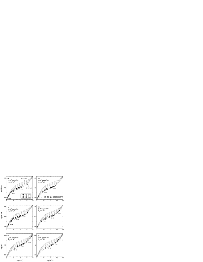
Figure 7: Results of our calculation of the molecular hydrogen cloud model for various intensities of the incident radiation $I_{0}$ and total molecular hydrogen column densities $N_{tot}$. The squares, circles, and asterisks indicate the equivalent widths of the lines from the $J=2,3,4$ levels, respectively. The filled and open symbols represent the results of our calculation, respectively, without and with thermalization of the velocity distribution at the level. The following distribution parameters were chosen: $b_{th}=0.8\,\mbox{km/s}$, $b_{turb}=1.6\,\mbox{km/s}$. The dashed lines represent the standard curves of growth with parameters $b$ from 1.8 to $3.8\,\mbox{km/s}$ at steps of $0.5\,\mbox{km/s}$. In the absence of a broadening effect, all symbols would fall on the lower standard curve of growth with $b=1.8\,\mbox{km/s}$.

As the result of our calculation, Fig. 7 presents the dependences of the line profiles for the Lyman and Werner molecular hydrogen bands on the depth of radiation penetration into the cloud. The line profiles reflect the particle velocity distribution on the line of sight at these levels and are calculated consistently. To present our results, we chose several lines for which the equivalent width was calculated and plotted on the curve of growth. For comparison with the observational data for the absorption system of QSO 1232+082   , we used the transitions from the rotational $J=2$(squares), $J=3$(circles), and $J=4$ (asterisks) levels. Figure 7 present two extreme cases: the absence of thermalization (filled symbols) and complete thermalization at all levels (open symbols) for the chosen parameters $b_{th}$ $b_{turb}$.

As was shown above, one might expect a significant broadening of the particle velocity distribution (by almost a factor of 2 in terms of the effective Doppler parameter) in the three-level system. However, the broadening of the distribution in the cloud model decreases appreciably. The main reason is that there are many radiative population transitions. For the chosen rotational level, there are about 60 such transitions in the Lyman or Werner bands. Each of these transitions has its own values of $\lambda f$ the product of the transition wavelength by the oscillator strength. For each of them, the broadening effect will begin (with line saturation) and be suppressed (when the Lorentz wings appear) at different depths in the cloud. This is easy to understand, since the optical depth includes the combination $N\lambda f$. Therefore, the incompletely broadened distributions from some transitions and the distributions with the influence of the Lorentz wings (reducing the broadening) from other transitions will be admixed to the maximum broadening of the distribution from some transition at some depth.

In addition to the aforesaid, the situation will be complicated at a high intensity of the incident radiation. In this case, the excited rotational levels will be populated more heavily than the ground levels until the lines of various transitions become saturated and the photoexcitation rate decreases. This will be true for the cloud shell. We will consider the peculiarity that arises in this case below.

When the curve of growth is analyzed, it is necessary that the lines from the levels with a broadening fall on the logarithmic segment of the curve of growth. Otherwise, if the broadening is present, we will not see it on the linear and square-root segments due to the peculiarity of the curve of growth. Therefore, when the system of molecular hydrogen is considered, the dependence in the manifestation of the broadening effect on the intensity of the radiation incident on the cloud is obvious. The excited rotational levels will be populated more heavily with increasing intensity of the incident radiation. This is clearly seen if we compare panel (a) in Fig. 7 with panels (c) and (e) (and panel (b) with panels (d) and (f)). In this case, the points corresponding to the transitions from different rotational levels become closer to one another (cf. the squares, circles, and asterisks).

The broadening effect in the chosen six combinations of parameters reaches its maximum at $N_{tot}=10^{18}\,\mbox{cm}^{-2}$, $I_{0}=10^{-17}\,\mbox{erg/cm}^{2}\mbox{/s/Hz}$ (panel (c) in Fig. 7). This can be explained as follows: the total hydrogen column density $N_{tot}$ should not be high ($>10^{19}\,\mbox{ }^{-2}$); otherwise, the Lorentz wings begin to suppress the effect (see Figs. 7b, 7d, and 7f). Obviously, the radiation must be intense enough for the excited rotational levels to fall into the region where the logarithmic part of the curve of growth begins, where the effect is most pronounced. If the intensity is higher, then the excited levels are populated more heavily (Fig. 7e) and approach the square-root part of the curve of growth; if the intensity is lower (Fig. 7a), then the levels fall on the linear part of the curve of growth. On these segments of the curve of growth, the broadening effect does not manifest itself, because it is insensitive to $b$.

However, the transfer of directional radiation that we considered is not enough to explain the broadening of the distribution for excited rotational levels of molecular hydrogen that arises in the absorption system of QSO 1232+082. Therefore, additional possibilities for the explanation should be sought. Nevertheless, this effect cannot be neglected, provided that the radiation directionality in the cloud is dominant.

The Influence of Dust

One of the ways to explain the broadening of the velocity distribution is the formation of molecular hydrogen on dust (Lacour et al. (2005)). However, the dust-related broadening effect during the propagation of directional radiation can be only a small correction. When a stationary situation is considered, the amount of formed hydrogen is assumed to be exactly equal to the amount of dissociated one, which accounts for 13% of the molecules excited in the Lyman or Werner bands. The remaining 87% are involved in radiative pumping, which, as was shown above, leads to a broadening of the distribution. This means that the two effects will be added with weights of 0.87 and 0.13 for the broadenings caused by radiative pumping and dust formation, respectively, relative to the distribution functions.

The presence of dust in the cloud can lead to a slightly different effect. The point is that dust reduces the intensity in the continuum. In fact, the population by the Lorentz wings also takes place in the continuum. Therefore, in the presence of dust in the cloud, it is capable of eating away the ultraviolet continuum in such a way that starting from some hydrogen column density $N_{d}$ (depending on the dust number density in the cloud), it essentially will reduce the population in the Lorentz wings to zero, i.e., in an ideal case, it will only freeze the broadening. We considered this additional effect, but it will not allow us to obtain the additional broadening needed to explain the observational data.

The Model of a Hot Shell

The assertion of Noterdaeme et al. (2007) that the velocity distribution at excited rotational levels can be broadened in the presence of a photodissociation region seems the most realistic explanation. This explanation naturally also arose in our paper when we considered the results of our model calculation presented in Fig. 8.

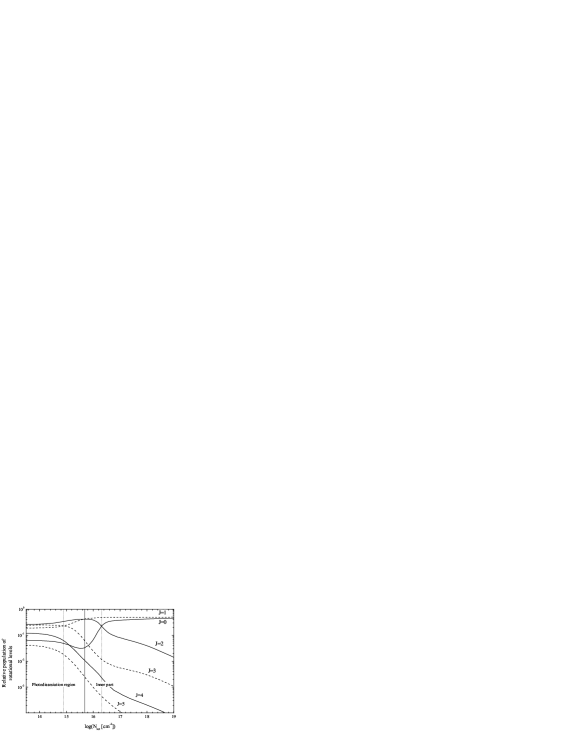
Figure 8: Populations of various rotational levels versus depth of penetration into the cloud. The cloud is arbitrarily separated by the vertical solid line into the shell (photo-dissociation region) and the inner part. The dotted vertical lines mark the depths at which the $J=1$ and $J=3$ (orthohydrogen) populations and the $J=0$ and $J=2$ (parahydrogen) populations become equal.

In Fig. 8, the populations of various rotational levels are plotted against the depth of radiation penetration into the cloud. We see from the figure that the cloud can be arbitrarily separated into two regions: the shell and the inner part. In the shell, the lines of the Lyman and Werner bands are not saturated and the radiative pumping rate is high at a sufficiently high intensity (in our case, $I_{0}=10^{-17}\,\mbox{ers/cm}^{2}\mbox{/s/Hz}$). Consequently, the transition rates between the rotational levels of molecular hydrogen in the lower vibrational (ground) electronic state are also high. In that case, the excited rotational levels will be populated significantly (the $J=2$, $3$ and $4$ levels are populated more heavily than the ground ones). Since the absorption lines become saturated as the radiation penetrates into the cloud (starting from $N_{tot}\approx 10^{15}\,\mbox{cm}^{-2}$), the photoexcitation rates and, hence, the population of the excited rotational levels decrease. As a result, only the ground levels turn out to be populated inside the cloud (in our case, $N_{tot}\gtrsim 10^{16}\,\mbox{cm}^{-2}$).We also see that the inner part of a cloud with $N_{tot}>10^{18}\,\mbox{cm}^{-2}$ (measured in the molecular hydrogen column density) will be several orders of magnitude larger than its shell. Therefore, the ground levels manifest themselves and allow us to determine the physical conditions only in the inner part of the cloud. As regards the excited levels, the column density of the excited rotational levels in the shell and the inner part of the cloud may turn out to be comparable in view of the radiative population pattern. This means that the excited rotational levels will reflect the physical conditions in the shell.

Since the photoexcitation rates in the shell are higher, the photodissociation rates are also higher. Photodissociation can heat the medium, because an energy of $4,48$ eV is released in one act of this process. Therefore, in the regions with active photodissociation, the medium can heat up and, as a result, have a broader velocity distribution of the molecules. These are called photodissociation regions (PDRs) (see, e.g., Hollenbach & Tielens (1999), Le Petit et al. (2006)).

We will take into account the PDR by specifying a nonuniformity of the Doppler parameter $b$ in the cloud. The medium in the shell will have a higher value of $b$ than that inside the cloud. In general, $b$ can increase in the shell not only through an increase in $b_{th}$, i.e., the heating of the medium, but also through an increase in the turbulent velocity component $b_{turb}$. To specify the gradient in $b$, we will take into account the fact that the photodissociation rate (and, hence, the heating of the medium) is related to the photoexcitation rate. The dependence of $b$ on the depth of penetration into the cloud that we chose is shown in Fig. 9. We chose the characteristic depth at which the shell inner part transition occurs to be $N_{tot}=3\times 10^{16}\,\mbox{cm}^{-2}$.

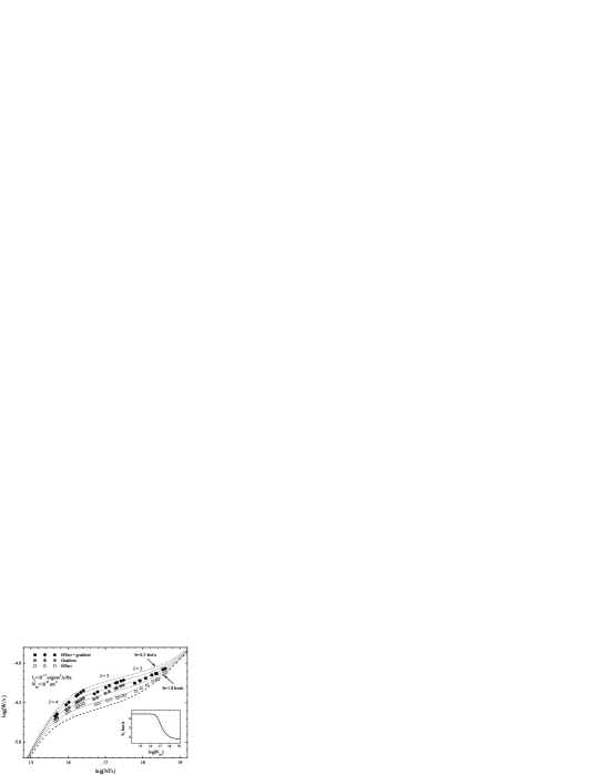
Figure 9: Results of our calculation of the molecular cloud model in the presence of a hot shell introduced through a nonuniformity of $b$ over the cloud (shown in the insert). The filled, open, and crossed symbols indicate the results of our calculation, respectively, without and with the shell and with a nonuniformity of $b$ but without any nonequilibrium radiative population. The dashed lines indicate the standard curves of growth with parameters b from 1.8 to $3.8\,\mbox{km/s}$ at steps of $0.5\,\mbox{km/s}$.

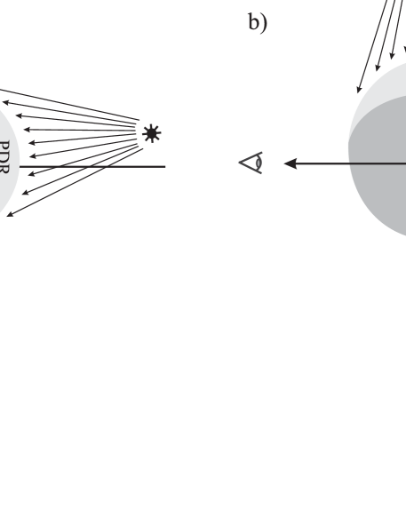
Figure 10: Possible geometric configurations of PDRs relative to the line of sight: (a) the line of sight is directed toward the source (a young star, a quasar) and, therefore, a PDR can be observed; in this case, the broadening effect should be taken into account; (b) the line of sight is perpendicular to the direction of the star and the manifestation of a PDR in observations is unlikely; in this case, the broadening effect is suppressed.

Figure 9 presents the results of our calculation of the model for radiative transfer in a molecular hydrogen cloud with a PDR specified by a nonuniformity of the parameter $b$. The open symbols indicate the equivalent widths of the lines from various rotational H₂ levels obtained without including the PDR but in the presence of a nonequilibrium radiative population (this calculation was presented above, in Fig. 7, panel (d)). The filled symbols represent the results of our calculation when adding a $b$ nonuniformity shown in the insert in Fig. 9. We see that the line equivalent widths for the transitions from excited rotational levels in the presence of a $b$ nonuniformity lie high, near the curves of growth with $b\sim 4.0\,\mbox{km/s}$. This result shows that the presence of a PDR can be used to explain the observational data for the absorption system of QSO 1232+082. Because of the simplified scheme of our calculation, we did not attempt to determine the exact parameters of the nonuniformity but only show the importance of taking into account the PDR.

We also see from Fig. 9 that when applying an analysis of the standard curve of growth to the computed points in the presence of a PDR (filled symbols), to achieve correspondence to some standard curve of growth, it will be necessary to displace the points greatly leftward. This will lead to an even larger increase in the effective parameter $b$ and larger errors in the populations of excited rotational levels. Therefore, it is important to note that assigning the same Doppler parameter to all rotational levels of molecular hydrogen when analyzing the absorption systems can lead to serious systematic errors in the column density and other physical parameters.

The crossed symbols indicate the results of our calculation in the absence of any nonequilibrium radiative population, i.e., the velocity distributions at all rotational levels were assumed to correspond to a Maxwellian distribution with a nonuniform $b$ over the cloud. We see that the effect should be taken into account for a detailed analysis of PDRs. If we associate the presence of a PDR with the location of the cloud near a young bright star, then this effect should be taken into account, because, in this case, the radiation can be assumed to be directional, i.e., to propagate near the line of sight. The point is that a PDR close to a star must be located in the cloud on the side of the star (see Fig. 10a). In the opposite case, where the young star cloud line is perpendicular to the line of sight, the effect of a nonequilibrium radiative population will be unobservable on the cloud. However, in this geometry, the PDR is also difficult to observe, because the molecular hydrogen column density is low ($N_{0}<10^{15}\,\mbox{cm}^{-2}$) in this region (see Fig. 10b). In this case, if the line of sight passes through the PDR, then it will not pass through the cloud interior, where the bulk of the molecular hydrogen is concentrated, and, conversely, if the line of sight passes through the interior, it will not touch the PDR.

CONCLUSIONS

Observations of molecular hydrogen clouds reveal a broadening of the velocity distribution at excited rotational levels. This effect is present in the observational data for Galactic (Jenkins & Peimbert (1997), Lacour et al. (2005)) and high-redshift (Noterdaeme et al. (2007)) clouds. We suggested a mechanism that could be responsible for the effective broadening of the distribution at excited rotational levels. The condition for the manifestation of this effect is radiation directionality. Using a three-level model system, we showed that the radiative pumping of an excited level for directional radiation could lead to a broadening of the particle velocity distribution at this level. The broadening of the distribution was considered in two limits: with thermalization of the velocity distribution (the turbulent component is retained) and without its thermalization. In the absence of thermalization, our mechanism in the three-level system considered (at transition line parameters typical of molecular hydrogen) can lead to an almost twofold effective broadening of the distribution in an analysis using the curve-of-growth method. The suppression of the effect during thermalization depends on the ratio of $b_{turb}$ and $b_{th}$, the parameters of the Maxwellian distribution attributed to turbulence and thermal motions

We applied the inferred effect to the system of molecular hydrogen energy levels and calculated a simple molecular hydrogen cloud model. We considered the balance at the excited rotational levels of the lower vibrational ground electronic state by taking into account the set of lines of the Lyman and Werner bands through which the radiative pumping proceeds. We also took into account the presence of a ro-vibrational cascade in the ground electronic state. The large number of lines slightly reduces the effect, because its manifestation in the radiative level population is heterogeneous. However, the broadening of the velocity distribution of molecules during radiative pumping is not enough to explain the data on the broadening of the distribution at excited rotational levels obtained by analyzing the absorption system of QSO 1232+082. Based on the calculated populations of rotational levels with depth, we assumed an additional mechanism capable of producing an effective broadening. This mechanism is related to the possibility of describing a molecular cloud by two different regions: the shell and the inner part. This separation, which naturally arises when the radiative transfer is considered in the cloud, stems from the fact that the excited and ground rotational levels are mostly populated in the shell and the inner part, respectively. In that case, the shell will be a PDR in which the influence of ultraviolet photons on the chemical composition and thermodynamic balance of the medium is strong. In view of the assumptions made in our model, we introduced a spatial nonuniformity of the Doppler parameter $b$ to take into account the PDR. The increase in $b$ in the shell is related to the heating of the medium or to the stronger turbulence. With a nonuniform parameter $b$, we can obtain the broadenings of the distributions at excited rotational levels needed to explain the observational data. A similar broadening mechanism for the velocity distributions of molecules was used by Noterdaeme et al. (2007). However, they did not consider the effect that we showed and that is related to radiation directionality. We point out that when a PDR manifests itself in the observations, the radiation directionality effect should also manifest itself. Therefore, in the case of a PDR region, it should be taken into account to eliminate the systematic error when the observational data are analyzed.

1 ACKNOWLEDGMENTS

This work was supported by the Russian Foundation for Basic Research (project no. 08-02-01246-a) and the Program of the Russian President for Support of Scientific Schools (project no. NSh-2600.2008.2).

APPENDIX

To derive the distribution thermalization while the turbulent component is retained, we will assume that that the distribution at the ground level in (5) is an equilibrium one and use the assumption about microturbulence. We can then write

$$n_{l}(v_{z},z)=\frac{n_{0}(z)}{A_{l}}P_{0k}(v_{z},z)\int\limits_{-\infty}^{+\infty}dv_{t}\,w_{turb}(v_{t})w_{th}(v_{z}-v_{t}),$$ (22)

where $n_{0}(z)$ is the number density at the ground level and $P_{0k}$ is defined by Eq. (2); $w_{turb}$ and $w_{th}$ are the Gaussian functions with parameters $b_{turb}$ and $b_{th}$ , respectively. Here, we used the fact that the particle velocity distribution was a convolution of the thermal and turbulent distributions.

Integrating Eq. (22) over $v_{z}$ yields

$$n_{l}(z)=\frac{n_{0}(z)}{A_{l}}\int\limits_{-\infty}^{+\infty}dv_{t}\int\limits_{-\infty}^{+\infty}dv_{z}\,w_{turb}(v_{t})w_{th}(v_{z}-v_{t})P_{0k}(v_{z},z).$$ (23)

We thus see that the distribution of the upward thrown particles in turbulent velocity is

$$w^{\prime}_{turb}(v_{t},z)=\frac{n_{0}(z)}{n_{l}(z)}\frac{1}{A_{l}}w_{turb}(v_{t})\times\\ \times\int\limits_{-\infty}^{+\infty}dv_{z}\,w_{th}(v_{z}-v_{t})P_{0k}(v_{z},z).$$ (24)

Under our assumptions, this nonequilibrium turbulent distribution is retained. Thus, after the thermalization of the medium, the particle distribution at level $l$ can bewritten as

$$\tilde{n}_{l}(v_{z},z)=n_{l}(z)\int\limits_{-\infty}^{+\infty}dv_{t}\,w^{\prime}_{turb}(v_{t},z)w_{th}(v_{z}-v_{t}).$$ (25)

Substituting (24) here, we obtain

$$\tilde{n}_{l}(v_{z},z)=\frac{n_{0}(z)}{A_{l}}\int\limits_{-\infty}^{+\infty}dv^{\prime}_{z}\,P_{0k}(v^{\prime}_{z},z)\times\\ \times\int\limits_{-\infty}^{+\infty}dv_{t}\,w_{th}(v^{\prime}_{z}-v_{t})w_{turb}(v_{t})w_{th}(v_{z}-v_{t}).$$ (26)

Integration over $v_{t}$ yields the product of twoGaussian functions with parameters $b$ and $b_{+}=\sqrt{b^{2}_{0}+b^{2}_{th}}=b_{th}\sqrt{1+(b_{turb}/b)^{2}}$.

Equations (26) and (23) then give (6).

References

- Abgrall et al. (1992) Abgrall H., Le Bourlot J., Pineau Des Forets G., et al., Astron. Astrophys. 253, 525, (1992).
- (2) Abgrall H., Roueff E., Launay F., et al., Astron. Astrophys. Suppl. Ser. 101, 273, (1993 ).
- (3) Abgrall H., Roueff E., Launay F., et al., Astron. Astrophys. Suppl. Ser. 101, 323, (1993 ).
- Bluhm et al. (2003) Bluhm H., de Boer K. S., Marggraf O., et al., Astron. Astrophys. 398, 983 (2003)
- Varshalovich et al. (2001) Varshalovich D.A., Ivanchik A.V., Petitjean P., Astron., letters 27, 803 (2001)
- Dalgarno & Black (1974) Dalgarno A. & Black J.H., Astrophys.J. 203, 132, (1974).
- Jenkins & Peimbert (1997) Jenkins E. B. & Peimbert A., Astrophys. J. 477, 265, (1997).
- Ge & Bechtold (1999) Ge J. & Bechtold J., APS confirence series 156, L121, (1999)
- Draine (1978) Draine B.T., Astrophys.J. Suppl. Ser. 36, 595, (1978)
- Ivanchik et al. (2005) Ivanchik A., Petitjean P., Varshalovich D., et al. Astron. Astrophys. 440, 45, (2005)
- Lacour et al. (2005) Lacour S., Ziskin V., Hebrard G., et al., Astrophys. J. 627, 251, (2005).
- Le Petit et al. (2006) Le Petit F., Nehme C., Le Bourlot J., et al., Astrophys. J. Suppl. Ser. 164, 506, (2006).
- Levshakov & Varshalovich (1985) Levshakov S.A. & Varshalovich D.A., MNRAS 212, 517 (1985)
- Ledoux et al. (2003) Ledoux C., Petitjean P., Srianand R., et al., MNRAS 346, 209, (2003)
- Noterdaeme et al. (2007) Noterdaeme P., Ledoux C., Petitjean P., et al., Astron. Astrophys. 474, 393, (2007).
- Noterdaeme et al. (2008) Noterdaeme P., Ledoux C., Petitjean P., et al., Astron. Astrophys. 481, 327, (2008).
- Petitjean et al. (2000) Petitjean P., Srianand R., Ledoux C., et al., Astron. Astrophys., 364, L26 L30 (2000)
- Rachford et al. (2002) Rachford B.L., Snow T. P., Tumlinson J., et al., Astrophys.J. 577, 221 (2002)
- Spitzer & Cochran (1973) Spitzer L. J. & Cochran W. D., Astropsyh.J. 186, 23, (1973).
- Stecher & Williams (1967) Stecher T.P. & Williams D.A., Astrophys.J. 149, 29, (1967).
- Savage et al. (1977) Savage B.D., Bohlin R. C., Drake J. F., et al., Astrophys.J. 216, 291 (1977)
- Tumlinson et al. (2002) Tumlinson J., Shull J. M., Rachford B. L., et al., Astrophys.J. 556, 857 (2002)
- Hollenbach et al. (1971) Hollenbach D.J., Werner M.W., Salpeter E.E., Astrophys.J. 163, 155, (1971).
- Hollenbach & Tielens (1999) Hollenbach D.J., Tielens A.G.G.M., Rev. Mod. Phys., 71, 1, (1999)
- Shull & Beckwith (1982) Shull J.M. & Beckwith S., Ann. Rev. Astron. Astrophys. 20, 163, (1982)
- Shull et al. (2000) Shull J.M., Tumlinson J., Jenkins E. B., et al., Astrophys.J. 538, 73 (2000)
- Srianand et al. (2008) Srianand R., Noterdaeme P., Ledoux C., et al., Astron. Astrophys. 482, L39 (2008)
- Srianand et al. (2005) Srianand R., Petitjean P., Ledoux C., et al., MNRAS 362, 549, (2005)
- (29) Jura M., Astrophys. J. 197, 575, (1975 ).
- (30) Jura M., Astrophys. J. 197, 581, (1975 ).