Selective spin transport through a quantum heterostructure: Transfer matrix method

Abstract

In the present work we propose that a one-dimensional quantum heterostructure composed of magnetic and non-magnetic atomic sites can be utilized as a spin filter for a wide range of applied bias voltage. A simple tight-binding framework is given to describe the conducting junction where the heterostructure is coupled to two semi-infinite one-dimensional non-magnetic electrodes. Based on transfer matrix method all the calculations are performed numerically which describe two-terminal spin dependent transmission probability along with junction current through the wire. Our detailed analysis may provide fundamental aspects of selective spin transport phenomena in one-dimensional heterostructures at nano-scale level.
Keywords: Quantum heterostructure, Selective spin transport, Junction current, Spin polarization, Transfer matrix method, Tight-binding framework.

I Introduction

Rapid progress of nanoscience and nanotechnology has allowed us to establish astonishing magneto devices which reveal several enchanting phenomena r1 . This new span in the study of magnetism has been instigated in 1988 after the discovery of Giant Magneto Resistance (GMR) effect r2 detected in magnetic multilayers formed by alternating magnetic and non-magnetic (NM) materials.

It is well known that in the absence of an external magnetic field, exchange coupling between neighboring magnetic layers through the non-magnetic one aligns the magnetization vector anti-parallel to each other. Then, when a strong magnetic field which is enough to overcome the anti-ferromagnetic coupling is applied, all the magnetization vectors orient along the field direction. This new parallel configuration yields an electrical resistance which is much smaller compared to the anti-ferromagnetic configuration. This substantial change in resistance is known as the GMR effect which is demonstrated in Fig. 1. We can define GMR mathematically as,

$$R=\frac{R_{AP}-R_{P}}{R_{P}}$$ (1)

where the symbols have their usual meanings. In conventional GMR effect, $R_{AP}>R_{P}$, and $R$ is unbounded. Another definition can also be given for GMR which is,

$$R^{\prime}=\frac{R_{AP}-R_{P}}{R_{AP}},$$ (2)

where, $0\leq{R^{\prime}}\leq 1$.

Along with this, the inverse GMR effect has also been discovered in some materials for which $R_{P}>R_{AP}$. The study of GMR effect is of underlying importance as it confirms the fact that the spin of an electron can also take a salient role in transport phenomena. In contrast with the past, the study of GMR effect has drawn much curiosity from academic circuit to commercial levels r3 as GMR based magnetic data storage devices are used in almost all computers. Not only that, spintronics in low-dimensional systems furnishes some tangible advantages over bulk metals and semiconductors. In molecular systems, the traditional mechanisms for

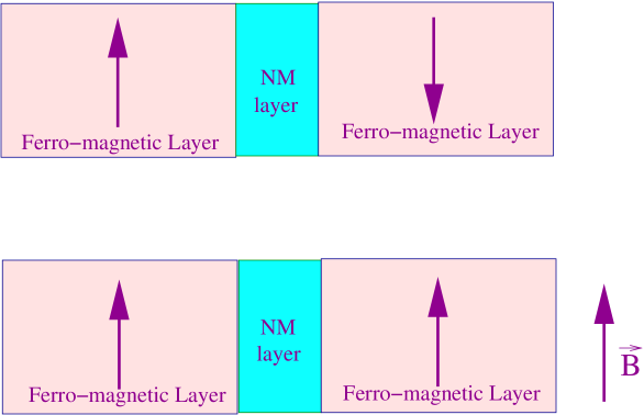
Figure 1: (Color online). Schematic representation of a GMR sensor.

spin decoherence (spin-orbit coupling, scattering from paramagnetic impurities, etc.) get reduced. Hence, in nano-scale systems, we can anticipate the spin coherence time to be several orders of magnitude larger than in bulk systems. Therefore, the study of spin dependent transport and spin dynamics is of pronounced importance to understand and to flourish the field, spintronics.

Spin dependent transport through mesoscopic systems has attracted affluent attention in the evolution of spintronics r4 ; r5 ; r6 ; r7 ; skm1 ; skm2 ; skm3 ; skm4 ; skm44 . Several experimental attempts have been done to study spin transport in quantum dots (QD) r8 ; r9 ; r10 ; r11 and other molecular systems r11 ; r12 ; r13 ; r14 . In these systems, electrical resistance depends on the spin state of electrons passing through the device, and it can be steered by an applied magnetic field. This is because of the misproportion in transmission probability for spin up and down electrons through the device r15 ; r16 , and, it can be utilized to achieve efficient spin filter, the design of which is of great concern in the present era of nanofabrication. Though much effort has been devoted to realize efficient spin filter and high degree of spin polarization, but none of them is quite suitable from experimental perspective. Therefore, it is major challenge to propose a simple model that can generate pure spin current and provide efficient spin filter operation, and also can be constructed through simple experimental set-up. Device with magnetic quantum dots (MQDs) can provide a possible route towards this direction.

The spin dependent transport through such a QD system can be inspected by coupling it to external electrodes and passing a current through the system r14 ; r17 ; r18 ; r19 ; r20 . Several theoretical as well as experimental studies have been made so far on spin transport through quantum dot devices r21 ; r22 ; r23 . Aim of our present model is to study coherent spin transport through a quantum heterostructure attached to two non-magnetic electrodes. Within a simple tight-binding framework we numerically calculate two-terminal spin dependent transmission probability together with junction current based on transfer matrix method r24 ; r25 ; r26 . Several cases are analyzed depending on the orientations of magnetic and non-magnetic sites of quantum heterostructure and our results suggest that under certain conditions the model can be utilized as an efficient spin filter with high degree of spin polarization ($100\%$) for a wide range of applied bias voltage.

The paper is organized as follows. In Sec. II, the model and the methods for the calculations of spin dependent transmission probabilities along with transport currents are described. In Sec. III we present the numerical results of heterostructure considering four different configurations and analyze how to achieve spin selective transmission and polarized spin currents. Finally, in Sec. IV we conclude our findings.

II Description of the model and theoretical formalism

II.1 The Model and the Hamiltonian

The model chosen is an array of quantum dots formed by a sequence of magnetic and non-magnetic sites connected to two non-magnetic leads, viz, source and

Figure 2: (Color online). Schematic view of magnetic quantum dot device (magnetic spacer) coupled to two leads, source and drain.

drain. The spin dependent electronic transport through this structure is studied including the spin flip scattering effect. The bridging conductor is basically a repetition of a chosen unit cell formed by magnetic and/or non-magnetic atoms. The geometry of the bridge structure is schematically shown in Fig. 2 which is further clearly viewed from 3. The direction of magnetization on each magnetic site in the MQD device is chosen to be arbitrary, specified in each site $n$, which in spherical

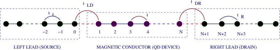
Figure 3: (Color online). Schematic view of the one-dimensional bridge system where magnetic conductor is connected to non-magnetic source and drain.

polar coordinate system is defined by two angles $\theta_{n}$ and $\phi_{n}$. Here $\theta_{n}$ is the angle between magnetization direction and the $Z$-axis, $\phi_{n}$ is the azimuthal angle of magnetization measured from $X$-axis at

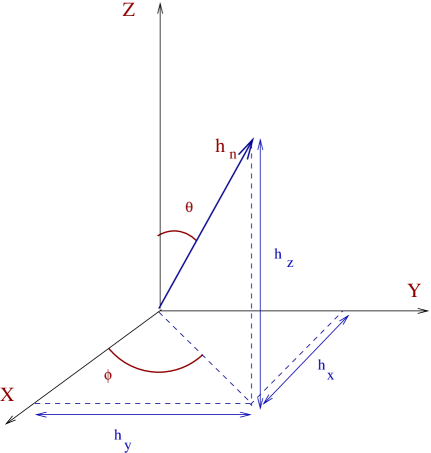
Figure 4: (Color online). Decomposition of $\vec{\bf h}_{n}$ in spherical polar coordinates.

site $n$ as shown in Fig. 4. The whole system can be described by a Hamiltonian like,

$$H=H_{L}+H_{LD}+H_{D}+H_{DR}+H_{R}$$ (3)

The spin polarized electrons for a $N$-site quantum dot can be described within the effective one-electron picture in tight-binding framework and the nearest-neighbor approximation as,

$$H_{D} = \sum_{n}{\bf c_{n}^{\dagger}}\left({\bf\epsilon}_{n}-\vec{\bf{h}_{n}}.\vec{\bf{\sigma}}\right)\bf c_{n}+\sum_{n}\left(\bf c^{{\dagger}}_{n}\bf t_{n,n+1}\bf c_{n+1}\right.$$ (4)

$$\left.+\bf c^{{\dagger}}_{n+1}\bf t_{n,n+1}\bf c_{n}\right)$$

where, $\bf c_{n}^{\dagger}=\left(\begin{array}[]{cc}c_{n\uparrow}^{{\dagger}}&c_{n\downarrow}^{{\dagger}}\end{array}\right)$,  
$\bf c_{n}=\left(\begin{array}[]{c}c_{n\uparrow}\\ c_{n\downarrow}\end{array}\right)$,  
${\bf\epsilon_{n}}=\left(\begin{array}[]{cc}\epsilon_{n\uparrow}&0\\ 0&\epsilon_{n\downarrow}\end{array}\right)$,  
$\bf t_{n,n+1}=\left(\begin{array}[]{cc}t_{n,n+1}&0\\ 0&t_{n,n+1}\end{array}\right)$ The term $\bf{\epsilon_{n}}$ of Eq. 4 describes the on-site energy. The term $\vec{\bf{h}_{n}}.\vec{\bf{\sigma}}$ describes the interaction of electrons with the magnetic atoms in MQD device. This term allows the spin flips at the magnetic sites. $h_{n}$ is the amplitude of the spin flip parameter at site $n$. $\bf{\sigma}$ is the Pauli spin operator having components $\bf{(\sigma_{x},\sigma_{y},\sigma_{z})}$. Spin flip scattering is dependent on the magnetic moment orientation of the atoms in MQD device with respect to the $Z$-axis. The term $t_{n,n+1}$ is the nearest-neighbor hopping integral, $c_{n\sigma}^{\dagger}(c_{n\sigma})$ is the creation(annihilation) operator for an electron on site $n$ with spin $\sigma$. The Hamiltonian of the left(right) lead is defined as,

$$H_{L(R)}=\sum_{i}{\bf c_{i}^{\dagger}\epsilon_{i}c_{i}}+\sum_{i}\left(\bf c^{{\dagger}}_{i}\bf t_{L(R)}\bf c_{i+1}+\bf c^{{\dagger}}_{i+1}\bf t_{L(R)}\bf c_{i}\right)$$ (5)

where $t_{L(R)}$ refers to the hopping integral between the sites of the left(right) lead. Finally, the Hamiltonian that corresponds to the coupling of the MQD device to the leads can be expressed in the form,

$$H_{LD(RD)} = \left(\bf c^{{\dagger}}_{0(N+1)}\bf t_{LD(RD)}\bf c_{1(N)}\right.$$ (6)

$$\left.+\bf c^{{\dagger}}_{1(N)}\bf t_{LD(RD)}\bf c_{0(N+1)}\right)$$

Throughout this study, it has been assumed that the nonmagnetic leads are ideal, i.e., their resistances have been neglected. The main contribution to the resistance in this ballistic device has come from contact resistance and spin scattering in MQD.

Using this model spin dependent transmission coefficients and junction currents are calculated to investigate the transport properties following transfer matrix approach. In this framework Schrödinger equation is written in terms of $\psi_{n,\sigma}$ (localized Wannier basis), which express the amplitude of wave function at site $n$, with energy $E$ and spin $\sigma$.

II.2 Transfer matrix method

In order to calculate spin dependent transmission probabilities, the Schrödinger equation for the electron wave function must be solved in the MQD device. So the starting point is the time independent Schrödinger equation in the MQD device, which can be written as,

$$H|\phi\rangle=E|\phi\rangle$$ (7)

where,

$$|\phi\rangle=\sum_{i}[\psi_{i\uparrow}|i\uparrow\rangle+\psi_{i\downarrow}|i\downarrow\rangle]$$ (8)

Here, $|\phi\rangle$ is written as a linear combination of spin up and spin down Wannier states. Now,

$$\vec{h}.\vec{\sigma} = h_{x}\sigma_{x}+h_{y}\sigma_{y}+h_{z}\sigma_{z}$$ (11)

$$= \left(\begin{array}[]{cc}h\cos\theta_{n}&h\sin\theta_{n}e^{-i\phi_{n}}\\ h\sin\theta_{n}e^{i\phi_{n}}&-h\cos\theta_{n}\end{array}\right)$$

So the Hamiltonian $H_{D}$ for the whole MQD device can be written as,

$$H_{D} = \sum_{n}\left(c^{{\dagger}}_{n\uparrow}c^{{\dagger}}_{n\downarrow}\right)\left(\begin{array}[]{cc}\epsilon_{n\uparrow}-h\cos\theta_{n}&-h\sin\theta_{n}e^{-i\phi_{n}}\\ -h\sin\theta_{n}e^{i\phi_{n}}&\epsilon_{n\downarrow}+h\cos\theta_{n}\end{array}\right)\left(\begin{array}[]{c}c_{n\uparrow}\\ c_{n\downarrow}\end{array}\right)+$$ (25)

$$\sum_{n}\left[\left(c{{}^{\dagger}}_{n\uparrow}c{{\dagger}}_{n\downarrow}\right)\left(\begin{array}[]{cc}t&0\\ 0&t\end{array}\right)\left(\begin{array}[]{c}c_{n+1,\uparrow}\\ c_{n+1,\downarrow}\end{array}\right)+\left(c{{}^{\dagger}}_{n+1,\uparrow}c{{\dagger}}_{n+1,\downarrow}\right)\left(\begin{array}[]{cc}t&0\\ 0&t\end{array}\right)\left(\begin{array}[]{c}c_{n,\uparrow}\\ c_{n,\downarrow}\end{array}\right)\right]$$

$$= H_{1}+H_{2}$$ (26)

where,

$$H_{1} = \sum_{n}|n\uparrow\rangle\left(\epsilon_{n\uparrow}-h\cos\theta_{n}\right)\langle n\uparrow|$$ (27)

$$- \sum_{n}|n\uparrow\rangle h\sin\theta_{n}e^{-i\phi_{n}}\langle n\downarrow|$$

$$- \sum_{n}|n\downarrow\rangle h\sin\theta_{n}e^{i\phi_{n}}\langle n\uparrow|$$

$$+ \sum_{n}|n\downarrow\rangle\left(\epsilon_{n\downarrow}+h\cos\theta_{n}\right)\langle n\downarrow|$$

$$H_{2} = \sum_{n}|n\uparrow\rangle t\langle n+1,\uparrow|+\sum_{n}|n\downarrow\rangle t\langle n+1,\downarrow|$$

$$+ \sum_{n}|n+1,\uparrow\rangle t\langle n\uparrow|+\sum_{n}|n+1,\downarrow\rangle t\langle n\downarrow|$$

Operating $H$ on $|\phi\rangle$ we get the following two equations relating the Wannier amplitudes on site $n$ of the MQD device with the neighboring $n\pm 1$ sites,

$$\left(E-\epsilon_{n}+h_{n}\cos\theta_{n}\right)\psi_{n\uparrow}+h_{n}\sin\theta_{n}e^{-i\phi_{n}}\psi_{n\downarrow}$$

$$=t\psi_{n+1,\uparrow}+t\psi_{n-1,\uparrow}$$ (29)

$$h_{n}\sin\theta_{n}e^{i\phi_{n}}\psi_{n\uparrow}+\left(E-\epsilon_{n}-h_{n}\cos\theta_{n}\right)\psi_{n\downarrow}$$

$$=t\psi_{n+1,\downarrow}+t\psi_{n-1,\downarrow}$$ (30)

Transfer matrix for the $n$th site relates the wave amplitudes of $n$th site with that of $(n-1)$th and $(n+1)$th sites. So we can write the transfer matrix equation for the $n$th site as,

$$\left(\begin{array}[]{c}\psi_{n+1\uparrow}\\ \psi_{n+1\downarrow}\\ \psi_{n\uparrow}\\ \psi_{n\downarrow}\end{array}\right) = \left(\begin{array}[]{cccc}\frac{E-\epsilon_{n}+h_{n}cos\theta_{n}}{t}&\frac{h_{n}sin\theta_{n}e^{-i\phi_{n}}}{t}&-1&0\\ \frac{h_{n}sin\theta_{n}e^{i\phi_{n}}}{t}&\frac{E-\epsilon_{n}-h_{n}cos\theta_{n}}{t}&0&-1\\ 1&0&0&0\\ 0&1&0&0\end{array}\right)$$ (44)

$$\times\left(\begin{array}[]{c}\psi_{n\uparrow}\\ \psi_{n\downarrow}\\ \psi_{n-1\uparrow}\\ \psi_{n-1\downarrow}\end{array}\right)$$

So the total transfer matrix for the whole MQD device can be written as, $P=\prod\limits_{l=N}^{1}P_{l}$
where,

$$P_{n}=\left(\begin{array}[]{cccc}\frac{E-\epsilon_{n}+h_{n}cos\theta_{n}}{t}&\frac{h_{n}sin\theta_{n}e^{-i\phi_{n}}}{t}&-1&0\\ \frac{h_{n}sin\theta_{n}e^{i\phi_{n}}}{t}&\frac{E-\epsilon_{n}-h_{n}cos\theta_{n}}{t}&0&-1\\ 1&0&0&0\\ 0&1&0&0\end{array}\right)$$ (45)

For the whole lead-MQD-lead system, the transfer matrix $\mathcal{T}$ that relates the wave amplitude from the left lead ($-1$th and $0$th sites) to the right lead ($(N+1)$th and $(N+2)$th sites) is given by,

$$\left(\begin{array}[]{c}\psi_{N+2\uparrow}\\ \psi_{N+2\downarrow}\\ \psi_{N+1\uparrow}\\ \psi_{N+1\downarrow}\end{array}\right)=\mathcal{T}\left(\begin{array}[]{c}\psi_{0\uparrow}\\ \psi_{0\downarrow}\\ \psi_{-1\uparrow}\\ \psi_{-1\downarrow}\end{array}\right)$$ (46)

where,

$$\mathcal{T}=M_{R}.P.M_{L}$$ (47)

Here, $M_{R}$ is the transfer matrix for right boundary, i.e., $(N+1)$th site. It relates the wave amplitudes from $N$th site (in the MQD device) to $(N+1)$th site (in the right lead). Similarly, $M_{L}$ represents the transfer matrix for left boundary, i.e., $0$th site. It relates the wave amplitudes from $1$st site (in the MQD device) to $-1$th site (in the left lead).

II.3 To calculate $M_{L}$ and $M_{R}$

Let us calculate $M_{L}$ first. For the left (or right) lead, $\vec{h}.\vec{\sigma}=0$. So the Hamiltonian for the lead (left or right) can be simplified as, $H_{\mbox{lead}}=H_{I}+H_{II}$, where,

$$H_{I}=\sum_{n}\left(|n\uparrow\rangle\epsilon_{n\uparrow}\langle n\uparrow|+|n\downarrow\rangle\epsilon_{n\downarrow}\langle\downarrow|\right)$$ (48)

and

$$H_{II} = \sum_{n}\left(|n\uparrow\rangle t\langle n+1,\uparrow|+|n\downarrow\rangle t\langle n+1,\downarrow|\right.$$ (49)

$$\left.+|n+1,\uparrow\rangle t\langle n\uparrow|+|n+1,\downarrow\rangle t\langle n\downarrow|\right)$$

We set $\epsilon_{n}=\epsilon_{0}$ for all $n$ in the leads. Now, from the time independent Schrödinger equation, operating $H$ on $|\phi\rangle$ we get two equations for $0$th site, relating the wave amplitudes of $1$st and $-1$th sites, as given below.

$$\left(E-\epsilon_{0}\right)\psi_{0\uparrow} = t_{LD}\psi_{1\uparrow}+t_{L}\psi_{-1\uparrow}$$

$$\left(E-\epsilon_{0}\right)\psi_{0\downarrow} = t_{LD}\psi_{1\downarrow}+t_{L}\psi_{-1\downarrow}$$ (50)

Now in the lead, according to the tight-binding model,

$$\psi_{n}=Ae^{ikna}$$ (51)

So $\psi_{-1}$ can be written in terms of $\psi_{0}$ as,

$$\psi_{-1}=\psi_{0}e^{-i\beta_{L}}$$ (52)

where, $\beta_{L}=ka$ and

$$E=\epsilon_{0}+2t_{L(R)}cos\beta_{L(R)}$$ (53)

From Eqs. 50, 51 and 52, $\psi_{1}$ can be expressed in terms of $\psi_{0}$ as,

$$\psi_{1}=\left(\frac{t_{L}}{t_{LD}}e^{i\beta_{L}}\right)\psi_{0}$$ (54)

Hence, the transfer matrix matrix equation for the $0$th site is of the form,

$$\left(\begin{array}[]{c}\psi_{1\uparrow}\\ \psi_{1\downarrow}\\ \psi_{0\uparrow}\\ \psi_{0\downarrow}\end{array}\right)=\left(\begin{array}[]{cccc}\frac{t_{L}}{t_{LD}}e^{i\beta_{L}}&0&0&0\\ 0&\frac{t_{L}}{t_{LD}}e^{i\beta_{L}}&0&0\\ 0&0&e^{i\beta_{L}}&0\\ 0&0&0&e^{i\beta_{L}}\end{array}\right)\left(\begin{array}[]{c}\psi_{0\uparrow}\\ \psi_{0\downarrow}\\ \psi_{-1\uparrow}\\ \psi_{-1\downarrow}\end{array}\right)$$ (55)

Similarly, from the time independent Schrödinger equation, operating $H$ on $|\phi\rangle$ we get two equations for $(N+1)$th site, relating the wave amplitudes of $N$th and $(N+2)$th sites as given below.

$$(E-\epsilon_{0})\psi_{N+1\uparrow} = t_{R}\psi_{N+2\uparrow}+t_{DR}\psi_{N-1\uparrow}$$

$$(E-\epsilon_{0})\psi_{N+1\downarrow} = t_{R}\psi_{N+2\downarrow}+t_{DR}\psi_{N-1\downarrow}$$ (56)

Exactly as before the transfer matrix matrix equation for the $(N+1)$th site can be written as,

$$\left(\begin{array}[]{c}\psi_{N+2\uparrow}\\ \psi_{N+2\downarrow}\\ \psi_{N+1\uparrow}\\ \psi_{N+1\downarrow}\end{array}\right)=\left(\begin{array}[]{cccc}e^{i\beta_{R}}&0&0&0\\ 0&e^{i\beta_{R}}&0&0\\ 0&0&\frac{t_{DR}}{t_{R}}e^{i\beta_{L}}&0\\ 0&0&0&\frac{t_{DR}}{t_{R}}e^{i\beta_{L}}\end{array}\right)\left(\begin{array}[]{c}\psi_{N+1\uparrow}\\ \psi_{N+1\downarrow}\\ \psi_{N\uparrow}\\ \psi_{N\downarrow}\end{array}\right)$$ (57)

Therefore,

$$M_{L} =$$ the transfer matrix for the left boundary (62)

$$= \left(\begin{array}[]{cccc}\frac{t_{L}}{t_{LD}}e^{i\beta_{L}}&0&0&0\\ 0&\frac{t_{L}}{t_{LD}}e^{i\beta_{L}}&0&0\\ 0&0&e^{i\beta_{L}}&0\\ 0&0&0&e^{i\beta_{L}}\end{array}\right)$$

$$M_{R} =$$ the transfer matrix for the right boundary (67)

$$= \left(\begin{array}[]{cccc}e^{i\beta_{R}}&0&0&0\\ 0&e^{i\beta_{R}}&0&0\\ 0&0&\frac{t_{DR}}{t_{R}}e^{i\beta_{L}}&0\\ 0&0&0&\frac{t_{DR}}{t_{R}}e^{i\beta_{L}}\end{array}\right)$$

II.4 To calculate the transmission probabilities of up and down spin electrons

Thus the transfer matrix for the whole system (lead-MQD-lead) can be written as,

$$\mathcal{T}=M_{R}.P.M_{L}$$ (68)

In order to calculate the transmission coefficient for the incident electrons with up or down spin using the transfer matrix method, the wave function amplitudes (Wannier amplitudes) have to be specified on proper atomic sites.

Case 1: Up spin incidence from the left lead
The eigenvalue equation involving the transfer matrix relating the Wannier amplitudes from sites $(N+2)$ and $(N+1)$ to sites $0$ and $-1$ is given by Eq. 46.
Let,
$\rho^{\uparrow\uparrow}$ = Reflection amplitude for up spin $(\uparrow)$ reflected as up spin $(\uparrow)$.
$\rho^{\uparrow\downarrow}$ = Reflection amplitude for up spin $(\uparrow)$ reflected as down spin $(\downarrow)$.
$\tau^{\uparrow\uparrow}$ = Transmission amplitude for up spin $(\uparrow)$ transmitted as up spin $(\uparrow)$.
$\tau^{\uparrow\downarrow}$ = Transmission amplitude for up spin $(\uparrow)$ transmitted as down spin $(\downarrow)$.
Now, for the left lead, the wave amplitudes at the sites 0 and -1 can be written as,

$$\psi_{-1\uparrow} = e^{-i\beta_{L}}+\rho^{\uparrow\uparrow}e^{i\beta_{L}}$$

$$\psi_{-1\downarrow} = \rho^{\uparrow\downarrow}e^{i\beta_{L}}$$

$$\psi_{0\uparrow} = 1+\rho^{\uparrow\uparrow}$$

$$\psi_{0\downarrow} = \rho^{\uparrow\downarrow}$$ (69)

Similarly, for the right lead, the wave amplitudes at the sites $(N+1)$ and $(N+2)$ become,

$$\psi_{N+2\uparrow}=\tau^{\uparrow\uparrow}e^{i(N+2)\beta_{R}}$$

$$\psi_{N+2\downarrow}=\tau^{\uparrow\downarrow}e^{i(N+2)\beta_{R}}$$

$$\psi_{N+1\uparrow}=\tau^{\uparrow\uparrow}e^{i(N+1)\beta_{R}}$$

$$\psi_{N+1\downarrow}=\tau^{\uparrow\downarrow}e^{i(N+1)\beta_{R}}$$ (70)

Therefore, the transfer matrix eigenvalue equation can be rewritten in terms of these wave function amplitudes as,

$$\left(\begin{array}[]{c}\tau^{\uparrow\uparrow}e^{i(N+2)\beta_{R}}\\ \tau^{\uparrow\downarrow}e^{i(N+2)\beta_{R}}\\ \tau^{\uparrow\uparrow}e^{i(N+1)\beta_{R}}\\ \tau^{\uparrow\downarrow}e^{i(N+1)\beta_{R}}\end{array}\right)=\mathcal{T}.\left(\begin{array}[]{c}1+\rho^{\uparrow\uparrow}\\ \rho^{\uparrow\downarrow}\\ e^{-i\beta_{L}}+\rho^{\uparrow\uparrow}e^{i\beta_{L}}\\ \rho^{\uparrow\downarrow}e^{i\beta_{L}}\end{array}\right)$$ (71)

Solving the above equation we can get the values of $\tau^{\uparrow\uparrow}$ and $\tau^{\uparrow\downarrow}$. The transmission coefficients $T^{\uparrow\uparrow}$ and $T^{\uparrow\downarrow}$ are defined as the ratio of the transmitted flux to the incident flux as,

$$T_{\uparrow\uparrow} = \frac{t_{R}\sin\beta_{R}}{t_{L}\sin\beta_{L}}|\tau^{\uparrow\uparrow}|^{2}$$

$$T_{\uparrow\downarrow} = \frac{t_{R}\sin\beta_{R}}{t_{L}\sin\beta_{L}}|\tau^{\uparrow\downarrow}|^{2}$$ (72)

Therefore, the total transmission probability for spin up is,

$$T_{\uparrow}=T_{\uparrow\uparrow}+T_{\uparrow\downarrow}$$ (73)

Case 2: Down spin incidence from the left lead
Similarly, for a down spin incidence from the left lead, the amplitudes at sites $-1$, $0$, $(N+1)$ and $(N+2)$ are given by,

$$\psi_{0\uparrow} = \rho^{\downarrow\uparrow}$$

$$\psi_{0\downarrow} = 1+\rho^{\downarrow\downarrow}$$

$$\psi_{-1\uparrow} = \rho^{\downarrow\uparrow}e^{i\beta_{L}}$$

$$\psi_{-1\downarrow} = e^{-i\beta_{L}}+\rho^{\downarrow\downarrow}e^{i\beta_{L}}$$ (74)

and

$$\psi_{N+2\uparrow} = \tau^{\downarrow\uparrow}e^{i(N+2)\beta_{R}}$$

$$\psi_{N+2\downarrow} = \tau^{\downarrow\downarrow}e^{i(N+2)\beta_{R}}$$

$$\psi_{N+1\uparrow} = \tau^{\downarrow\uparrow}e^{i(N+1)\beta_{R}}$$

$$\psi_{N+1\downarrow} = \tau^{\downarrow\downarrow}e^{i(N+1)beta_{R}}$$ (75)

So, as before, the transfer matrix equation for down spin incidence can be rewritten in terms of these wave amplitudes as,

$$\left(\begin{array}[]{c}\tau^{\downarrow\uparrow}e^{i(N+2)\beta_{R}}\\ \tau^{\downarrow\downarrow}e^{i(N+2)\beta_{R}}\\ \tau^{\downarrow\uparrow}e^{i(N+1)\beta_{R}}\\ \tau^{\downarrow\downarrow}e^{i(N+1)\beta_{R}}\end{array}\right)=\mathcal{T}.\left(\begin{array}[]{c}\rho^{\downarrow\uparrow}\\ 1+\rho^{\downarrow\downarrow}\\ \rho^{\downarrow\uparrow}e^{i\beta_{L}}\\ e^{-i\beta_{L}}+\rho^{\downarrow\downarrow}e^{i\beta_{L}}\end{array}\right)$$ (76)

This equation can be solved to compute $\tau^{\downarrow\downarrow}$ and $\tau^{\downarrow\uparrow}$. The transmission coefficients $T^{\downarrow\downarrow}$ and $T^{\downarrow\uparrow}$ are defined by the ratio of the transmitted flux to the incident flux as,

$$T_{\downarrow\downarrow} = \frac{t_{R}\sin\beta_{R}}{t_{L}\sin\beta_{L}}|\tau^{\downarrow\downarrow}|^{2}$$

$$T_{\downarrow\uparrow} = \frac{t_{R}\sin\beta_{R}}{t_{L}\sin\beta_{L}}|\tau^{\downarrow\uparrow}|^{2}$$ (77)

Therefore, the total transmission probability for spin down is,

$$T_{\downarrow}=T_{\downarrow\downarrow}+T_{\downarrow\uparrow}$$ (78)

At low temperatures, the transport of such mesoscopic systems is ballistic and coherent. In this regime, transmitted spin dependent current flowing through the interacting region with arbitrary magnetic configurations, symmetrically attached to two NM leads is given by the relation r29 ; r30 ; r35 ,

$$I_{\sigma\sigma^{\prime}}(V)=\frac{e}{h}\int\left(f_{S}-f_{D}\right)T_{\sigma\sigma^{\prime}}(E)~{}dE$$ (79)

where, $f_{S(D)}=f\left(E-\mu_{S(D)}\right)$ gives the Fermi distribution function with the electrochemical potential $\mu_{S(D)}=E_{F}\pm eV/2$, $E_{F}$ being the equilibrium Fermi energy.

III Numerical results and discussion

Based on the above theoretical framework now we present our numerical results for NM/MQD/NM heterostructure. We assume that the MQD device is constructed by repeating a specific unit cell which is made up of some magnetic (A) and non-magnetic (B) atoms having different magnetic moment orientations. By applying an external magnetic field, the magnetization direction of the NM/MQD/NM system can be switched. Four different unit cell configurations are taken into account to reveal different aspects of spin dependent transport through a quantum heterostructure, and these results are critically analyzed below.

Before presenting the numerical results let us first mention the values of different parameters those are considered throughout our numerical calculations. For the sake of simplicity, the on-site energies both in the two leads and in MQD device are taken to be zero. The nearest-neighbor hopping integral $t_{n,n+1}$ ($=t$) in the MQD device is set to $1$, and, in the two side-attached leads the hopping strength $t_{L(R)}$ is also fixed at $1$. The spin flip parameter is chosen as $h=1$. To narrate the coupling effect r31 ; r32 ; r34 ; r344 we focus our results for the two limiting cases depending on the coupling strength between the MQD device to the source and drain leads. In one case we call it weak-coupling limit which is described by the condition $t_{LD(RD)}<<t$. For this regime we choose $t_{LD}=t_{RD}=0.2$. While the other case, called as strong-coupling limit, is defined by the condition $t_{LD(RD)}\sim t$, and here we set $t_{LD}=t_{RD}=0.8$. Throughout the analysis we choose the units $c=e=h=1$, for simplification, and set the electronic temperature of the system to zero.

Figure 5 presents the spin dependent transmission probabilities as a function of injecting electron energy $E$ for a specific unit cell configuration shown in (a), where the unit cell is made up of four $A$-type (magnetic) atoms and the moment of each atom is aligned along positive $Z$-direction. The net up and down spin probabilities ($T_{\uparrow}$ and $T_{\downarrow}$) for both the weak- and strong-coupling limits are computed and they are presented in (b) and (c), respectively, while in (d) we present spin flip transmission probabilities ($T_{\uparrow\downarrow}$ and $T_{\downarrow\uparrow}$). From the spectra it is observed that the transmission probability exhibits sharp resonant peaks in the limit of weak-coupling, while these peaks get broadened and achieve much higher value in the limit of strong-coupling. The contribution for the broadening of the resonant peaks appears from the broadening of energy levels of the MQD device in this strong-coupling limit. All these resonant

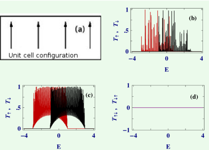
Figure 5: (Color online). Spin dependent transmission probabilities as a function of injecting electron energy $E$ for a $64$-site MQD device considering the unit cell configuration as given in (a). The unit cell is made up of four magnetic atoms $A$, each having parallel magnetic moment. The net up ($T_{\uparrow}$, red color) and down ($T_{\downarrow}$, black color) spin transmission probabilities for the weak-coupling limit are shown in (b), while these probabilities for the strong-coupling limit are given in (c). Spin flip transmission probabilities ($T_{\uparrow\downarrow}$ and $T_{\downarrow\uparrow}$) for both the weak- and strong-coupling limits are presented in (d).

peaks are associated with the energy eigenvalues of the bridging system, and thus, we can say that the transmission-energy spectrum manifests itself the electronic structure of the device sandwiched between two electrodes. Most interestingly we see from the spectra given in Figs. 5(b) and (c) that the MQD device can exhibit spin polarization for a wide range of energy. There is sharp energy shift between the up and down spin transmission spectra. For one energy region ($-3\leq E\leq-1$) only up spin electrons, while for the other region ($1\leq E\leq 3$) only down spin electrons are allowed to move from source to drain through the MQD device. Within the range $-1\leq E\leq 1$ the overlap between two transmission probabilities takes place. Thus setting the Fermi energy to a suitable energy zone ($-3\leq E\leq-1$ or $1\leq E\leq 3$) we can get either up or down spin transmission across the junction which yields a selective spin transmission. This is essentially what we expect from our model. For this model where all magnetic moments are aligned along $Z$-direction, the spin-flip transmission

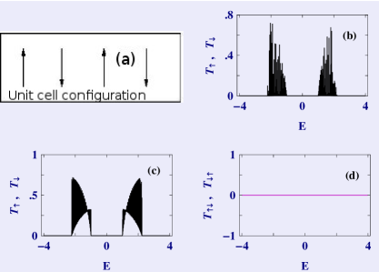
Figure 6: (Color online). Spin dependent transmission probabilities as a function of energy for a $64$-site MQD device where the unit cell, shown in (a), is made up of four magnetic atoms $A$, having anti-parallel magnetic moment. The spectra (b), (c) and (d) correspond to the identical meanings as described in Fig. 5.

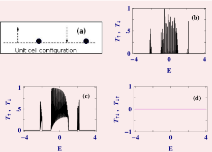
Figure 7: (Color online). Spin dependent transmission probabilities as a function of energy for a $64$-site MQD device where the unit cell, shown in (a), is made up of two magnetic atoms $A$, oriented in anti-parallel configuration, and two non-magnetic atoms $B$. The spectra (b), (c) and (d) correspond to the identical meanings as described in Fig. 5.

probability becomes zero for the entire energy region (see Fig. 5(d)). This can be explained through a simple mathematical argument. The term $\vec{\bf{h}}_{n}.\vec{\bf{\sigma}}$ in the Hamiltonian $H_{D}$ is responsible for spin flipping. Since all the moments are aligned along $Z$-direction, this terms simplifies to $h_{n}\sigma_{z}$, which is

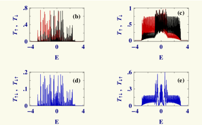
Figure 8: (Color online). Spin dependent transmission probabilities as a function of energy for a $64$-site MQD device where the unit cell, shown in (a), is made up of magnetic atoms $A$ those are oriented at an angle $\theta$ with respect to $Z$-axis. The net up ($T_{\uparrow}$, red color) and down ($T_{\downarrow}$, black color) spin transmission probabilities for the weak- and strong-coupling limits are shown in (b) and (c), respectively, while the spin-flip transmission probabilities ($T_{\uparrow\downarrow}$ and $T_{\downarrow\uparrow}$, they exactly overlap with each other) for these coupling limits are shown in (d) and (e), respectively. Here $\theta$ is fixed at $\pi/3$.

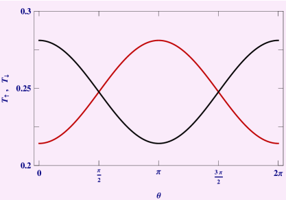
Figure 9: (Color online). $T_{\uparrow}$ (red curve) and $T_{\downarrow}$ (black curve) as a function of $\theta$ for a $64$-site MQD (all sites are magnetic) device in the strong-coupling limit for the typical energy $E=0.25$.

diagonal and does not contain spin-flip factors $\sigma_{+}$ and $\sigma_{-}$, associated with $\sigma_{x}$ and $\sigma_{y}$. Therefore, no spin-flip transmission is obtained for this configuration.

Now move to the device where all sites are magnetic ($A$-type), but the moments are aligned in a perfect anti-parallel configuration as shown in Fig. 6(a). The results for such a quantum device with $64$ sites are shown in Figs. 6(b)-(d), where different spectra correspond to the identical meanings as described in Fig. 5. Quite interestingly we notice that for this configuration both the up and down spin bands overlap with each other, and accordingly, spin polarization cannot be achieved. This band overlap can be easily understood from the Hamiltonian $H_{D}$ since up and down spin electrons experience exactly identical potential while traversing through the MQD device, and thus, the energy spectra for these two spin

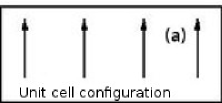
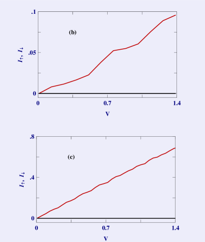
Figure 10: (Color online). Spin dependent currents ($I_{\uparrow}$ and $I_{\downarrow}$) as a function of bias voltage $V$ for a $64$-site MQD device considering the unit cell where all moments are aligned in a perfect parallel configuration (shown in (a)), where the red and black lines correspond to $I_{\uparrow}$ and $I_{\downarrow}$, respectively. (b) Weak-coupling limit and (c) strong-coupling limit. Here we set the Fermi energy $E_{F}=-2.0$.

cases are identical which yield identical transmission-energy spectra. Along with this we also find a gap in the spectrum across $E=0$. This is exactly what we get in a binary lattice model since for this configuration successive moments are aligned in anti-parallel configuration providing an equivalent binary lattice geometry. Like Fig. 5, here also we get vanishing spin flip transmission (Fig. 6(d)) as $\theta$ becomes $0$ or $\pi$ for the moments.

In Fig. 7 the results are given for another MQD device where two magnetic moments are separated by a non-magnetic one and the moments are oriented in perfect anti-parallel configuration. Similar to the previous case (i.e., Fig. 6) here also we do not get any separated spin channel and hence no spin polarization will be available. For this device the spectrum exhibits two finite gaps at the energy band edges associated with unit cell configuration, and like previous systems, spin flipping does not take place.

Finally, focus on the MQD device where all the sites are magnetic and they are oriented at a particular angle $\theta$ with respect to $Z$-axis. The unit cell configuration for such a system is schematically shown in Fig. 8(a) and the corresponding results are placed in Fig. 8(b)-(e). Here we set $\theta=\pi/3$. For this set-up spin polarization is achieved for a wide range of energy $E$, like the first configuration (Fig. 5), which is more clearly seen from the result of the strong-coupling case (Fig. 8(c)). Though the present configuration exhibits spin polarization for a large energy window, the degree of spin polarization is less compared to the

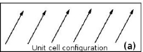
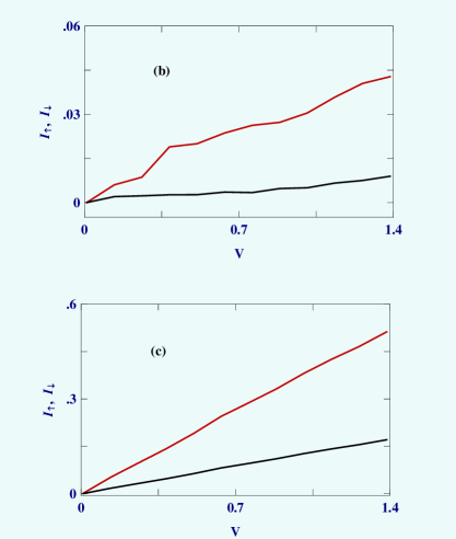
Figure 11: (Color online). Spin dependent currents ($I_{\uparrow}$ and $I_{\downarrow}$) as a function of voltage $V$ for a $64$-site MQD device where all the magnetic moments are aligned along a specific direction (as shown in (a)) making an angle $\theta$ with respect to $Z$-axis, where the red and black lines correspond to $I_{\uparrow}$ and $I_{\downarrow}$, respectively. (a) Weak-coupling limit and (b) strong-coupling limit. Here we choose $E_{F}=-2.0$ and $\theta=\pi/3$.

device where all the moments are aligned in a perfect parallel configuration (Fig. 5(a)). In the later case a perfect separation takes place between up and down spin channels yielding $100\%$ spin polarization, while for the device where moments are aligned in a particular direction making an angle $\theta$, an overlap between two channels takes place though the transmission amplitudes are different providing less degree of polarization. In addition we also find that for this MQD device spin-flip transmission is obtained (see Figs. 8(d) and (e)) and the appearance of spin-flip transmission probabilities can be easily understood from the spin-flip term $\vec{\bf h}_{n}.\vec{\bf\sigma}$ as in contains $\sigma_{+}$ and $\sigma_{-}$ through the components $\sigma_{x}$ and $\sigma_{y}$ which are responsible for spin flipping. Obviously we should expect more flipping with increasing the orientation angle $\theta$.

So now the question naturally comes how the net up and down spin probabilities get changed with $\theta$. To answer it in Fig. 9 we present the results of $T_{\uparrow}$ (red curve) and $T_{\downarrow}$ (black curve) as a function of $\theta$ for a MQD device, considering all sites are magnetic, at a typical energy $E=0.25$. It is interesting to see that for $\theta=0$ the difference between $T_{\uparrow}$ and $T_{\downarrow}$ becomes maximum (viz, maximum polarization) and it (the difference) gradually decreases to zero at $\theta=\pi/2$ (viz, no spin polarization). This difference starts increasing with the further increment of $\theta$ and eventually reaches to a maximum for $\theta=\pi$, reversing the sign of spin polarization compared to $\theta=0$. Thus a periodic variation is naturally expected as function of $\theta$ and it is also clearly reflected from the spectra.

All the basic features of spin dependent transmission probabilities together with spin polarization studied above become much more clearly visible from

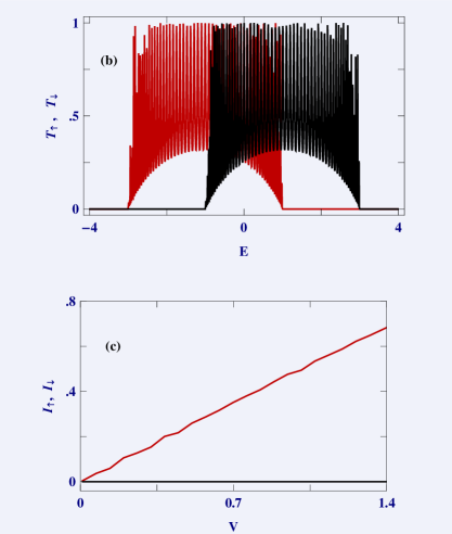
Figure 12: (Color online). Spin dependent transmission probabilities and corresponding currents for a MQD device considering odd number of magnetic sites ($N=65$) where all the magnetic moments are aligned in a perfect parallel configuration. All the results are computed for the strong-coupling limit where the curves with red and black colors represent the up and down spin cases, respectively. We set $E_{F}=-2.0$.

current-voltage characteristics. The current through the bridge system can be determined by integrating spin dependent transmission function over a suitable energy window, as prescribed in Eq. 79. Let us start with Fig. 10 where net up (red line) and down (black line) spin currents are shown as a function of bias voltage $V$ for a $64$-site MQD device in which all the magnetic moments are aligned in a perfect parallel configuration (viz, $\theta=0$). The results for the two different coupling cases are shown in (b) and (c), where all these currents are computed setting the Fermi energy $E_{F}=-2.0$ (the zone where only up spin electron can transmit, see Figs. 5(b) and (c)). In the limit of weak-coupling current provides step-like behavior, while it becomes quite

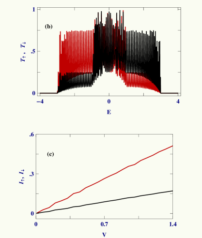
Figure 13: (Color online). Spin dependent transmission probabilities and associated currents for a MQD device considering odd number of magnetic sites ($N=65$) where all the magnetic moments are aligned along a specific direction (as shown in (a)) making an angle $\theta=\pi/3$ with respect to $Z$-axis. The spectra shown in (b) and (c) correspond to the identical meanings as described in Fig. 12 and they are computed for the same parameter values as taken in Fig. 12.

continuous in the limit of strong-coupling. It is solely associated with the transmission function as the current is computed by integrating this function. From these spectra the behavior of spin polarization can be clearly examined. It is observed that for the entire voltage window only up spin current (red line) is passing through the junction since the other current (black line) drops exactly to zero. Certainly, for this wide bias region the device exhibits $100\%$ spin polarization. So, the spin polarization efficiency defined by the condition $\eta=(|I_{\uparrow}-I_{\downarrow}|)/(I_{\uparrow}+I_{\downarrow})$ becomes unity. Exactly opposite scenario i.e., finite down spin current and vanishing up spin current across the junction, is obtained when the Fermi energy is fixed at $2.0$. Thus setting the Fermi energy to a suitable energy zone we can get selective polarized spin current with maximum efficiency $\eta=1$.

Since for the other two MQD devices, those are formed by repeating the unit cell configurations given in Figs. 6(a) and 7(a), up and down spin channels are not separated in energy scale we cannot expect spin polarization,

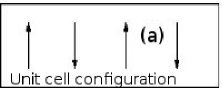
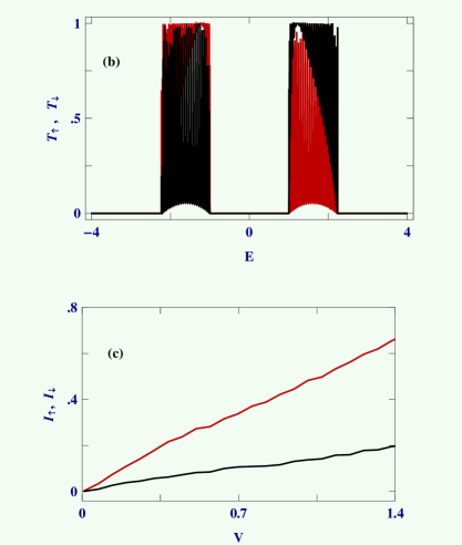
Figure 14: (Color online). Spin dependent transmission probabilities and corresponding currents for a MQD device considering odd number of magnetic sites ($N=65$) where the magnetic moments are arranged in perfect anti-parallel configuration (as shown in (a)), where the spectra (b) and (c) represent the similar meanings as described in Fig. 12 and they are computed for the identical parameter values as taken in Fig. 12. Here we assume that the magnetic moment at the end site of the chain (viz, $n=65$) is aligned along positive $Z$-axis.

and accordingly, we do not discuss the $I$-$V$ characteristics for these systems to save space. So finally move to the system where all the moments are aligned in a specific direction making an angle $\theta$ with respect to $Z$-direction. The results are shown in Fig. 11. Like Fig. 10 here also current exhibits step-like and continuous-like nature of current in the limit of weak and strong coupling cases, respectively. But as $\theta$ is finite ($\neq 0$ or $\pi$), a non-vanishing down spin current where the contribution comes from the spin flipping is obtained together with up spin current though their amplitudes differ significantly yielding a finite polarization, which is obviously less then $100\%$ (viz, $\eta<1$). The reverse scenario will also be obtained when the Fermi level is placed at $2.0$, which is not shown here to save space.

The results studied so far are worked out for a typical system size considering $N=64$ (even $N$). So one can think whether these features

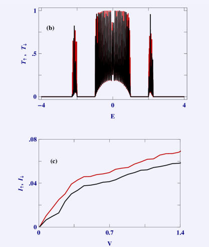
Figure 15: (Color online). Spin dependent transmission probabilities and associated currents for a MQD device considering odd number of magnetic sites ($N=65$) where the magnetic moments are arranged as shown in (a), and the other two spectra ((b) and (c)) represent the identical meanings as described in Fig. 12. The values of all physical parameters remain same as considered in Fig. 12, except $E_{F}$ which is set at $-2.15$. Here we also assume that the magnetic moment at the end site of the chain (viz, $n=65$) is aligned along positive $Z$-axis, like Fig. 14.

get changed for such MQD devices when the system size ($N$) becomes odd or remain same like what we get for the case of even $N$. To reveal this fact start with Fig. 12 where we present the results for a $65$-site ($N=65$) MQD device considering the perfect parallel alignment of all magnetic moments. In Fig. 12(b) we show the dependence of net up (red color) and down (black color) spin transmission probabilities, and the corresponding currents are placed in Fig. 12(c). Like Fig. 5(c) (where we set $N=64$) here also we find a clear separation between up and down spin transmission spectra (Fig. 12(b)), and the width of this energy separation is exactly identical to the previous case. This behavior is nicely reflected in the current-voltage characteristics (see Fig. 12(c)), similar to Fig. 10(c). Thus for this configuration, where all moments are aligned in a perfect parallel configuration, we expect identical behavior both for odd and even $N$.

In the same footing we can anticipate identical behavior for the MQD device where all the moments are arranged along a specific direction (Fig. 13(a)) making an angle $\theta$ with respect to $Z$-axis. The results are shown in Fig. 13 for a $65$-site magnetic system setting $\theta=\pi/3$, where all the other physical parameters kept unchanged as taken in Fig. 12. The transmission probabilities for both up and down spin electrons (Fig. 13(b)) look exactly identical what we get in Fig. 8(c) for a $64$-site system, and thus, spin dependent currents (Fig. 13(c)) exhibit identical variation like Fig. 11(c). Therefore, for this configuration we also get identical behavior irrespective of $N$.

But, some different features can be expected depending on even and odd $N$ for the other two configurations (Figs. 6(a) and 7(a)). The reason is that the magnetic moment of the last site breaks the symmetry between the potentials experienced by up and down spin electrons. And accordingly a finite spin polarization is obtained, though it becomes too small. The results are shown in Figs. 14 and 15 considering $N=65$, where we assume that the magnetic moment at the end site is aligned along the positive $Z$-direction which essentially makes the difference between up and down spin probabilities as well as currents. In both these two cases we get finite spin polarization as up spin current is higher than the other one (Figs. 14(c) and 15(c)). Exactly opposite scenario (viz, higher down spin current compared to the up spin current) is obtained when the orientation of the magnetic moment placed at the end site gets flipped from up to down viz, oriented along negative $Z$-direction.

IV Concluding remarks

To conclude, in the present work we explore spin dependent transport phenomena through a one-dimensional quantum heterostructure composed of magnetic and non-magnetic quantum dots. A simple tight-binding framework is given to describe the model where the heterostructure is coupled to two one-dimensional non-magnetic electrodes, and all the calculations are done based on transfer matrix method. Several cases are analyzed depending on the configuration of the bridging system. From our numerical results which describe two-terminal spin dependent transmission probabilities along with transport currents, we show that under certain condition $100\%$ spin polarization can be achieved for a wide range of bias voltage. Certainly, this is an important observation and can be utilized to design an efficient spin filter device in nano-scale level. Apart from this our detailed theoretical analysis based on transfer matrix method can be implemented quite easily to any spin based quantum structure to describe transport phenomena.

Throughout the presentation, we have made several important assumptions. Below we discuss briefly some of these approximations.

$\bullet$ All the calculations have been worked out at absolute zero temperature, but the physical picture studied above will not change at non-zero finite temperature as long as the thermal energy $(k_{B}T)$ is less than the average spacing of energy levels of the bridging material.

$\bullet$ The effect of electron-electron (e-e) correlation has not been taken into account. The inclusion of e-e correlation is a major challenge to us, since over the past few years much efforts have been made to incorporate this effect, but no proper theory has been well developed.

$\bullet$ Electron-phonon (e-ph) interaction has also been neglected in our theoretical formulation, as we are dealing with zero temperature. But even at finite temperature one can neglect this effect as the broadening of energy levels due to e-ph interaction is much smaller than the broadening caused by coupling of the MQD device with electrodes.

$\bullet$ All the results have been presented for ordered systems, but in presence of impurity transport properties can change which demands further study and we hope it will be available in our next work.

References

- (1) J. Stöhr and H. C. Siegmann, Magnetism-From fundamentals to Nanoscale Dynamics, Springer (2006).
- (2) S. Maekawa and T. Shinjo, Spin Dependent Transport in Magnetic Nanostructures, CRC PRESS (2002).
- (3) S. Sanvito, Ab-initio Methods for Spin Transport at Nanoscale level, Review Article (unpublished).
- (4) G. Prinz, Phys. Today 48, 58 (1995).
- (5) G. Prinz, Science 282, 1660 (1998).
- (6) S. A. Wolf, D. D. Awschalom, R. A. Buhrman, J. M. Daughton, S. von Molnár, M. L. Roukes, A. Y. Chtchekanova, and D. M. Treger, Science 294, 1488 (2001).
- (7) M. Ziese and M. J. Thornton, Spin Electronics, Springer, Berlin (2001).
- (8) S. K. Maiti, Eur. Phys. J. B 88, 172 (2015).
- (9) S. K. Maiti, Phys. Lett. A 379, 361 (2015).
- (10) M. Dey, S. K. Maiti, S. Sil, and S. N. Karmakar, J. Appl. Phys. 114, 164318 (2013).
- (11) M. Dey, S. K. Maiti, and S. N. Karmakar, J. Appl. Phys. 109, 024304 (2011).
- (12) M. Dey, S. K. Maiti, and S. N. Karmakar, J. Comput. Theor. Nanosci. 8, 253 (2011).
- (13) M. Stopa, J. P. Bird, K. Ishibashi, Y. Aoyagi, and T. Sugano, Phys. Rev. Lett. 76, 2145 (1996).
- (14) R. López and D. Sánchez, Phys. Rev. Lett. 90, 116602 (2003).
- (15) Z. H. Xiong, D. Wu, Z.V. Vardeny, and J. Shi, Nature 427, 821 (2004).
- (16) B. R. Bulka and S. Lipinski, Phys. Rev. B 67, 024404 (2003).
- (17) M. Zwolak and M. D. Ventra, Appl. Phys. Lett. 81, 925 (2002).
- (18) W. I. Babiaczyk and B. R. Bulka, J. Phys.: Condens. Matter 16, 4001 (2004).
- (19) R. Pati, L. Senapati, P. M. Ajayan, and S. K. Nayak, Phys. Rev. B 68, 100407 (2003).
- (20) A. A. Shokri and A. Saffarzadeh, J. Phys.: Condens. Matter 16, 4455 (2004).
- (21) A. A. Shokri and A. Saffarzadeh, Eur. Phys. J. B 42, 187 (2004).
- (22) S. K. Watson, R. M. Potok, C. M. Marcus, and V. Umansky, Phys. Rev. Lett. 91, 258301 (2003).
- (23) E. R. Mucciolo, C. Chamon, and C. M. Marcus, Phys. Rev. Lett. 89, 146802 (2002).
- (24) B. Wang, J. Wang, and H. Guo, Phys. Rev. B 67, 092408 (2003).
- (25) T. Chakraborty, Quantum Dots: A Survey of the Properties of Artificial Atoms, Elsevier, Amsterdam (1999).
- (26) M. Mardaani and K. Esfarjani, Physica E 25, 119 (2004).
- (27) M. Mardaani, A. A. Shokri, and K. Esfarjani, Physica E 28, 150 (2005).
- (28) A. A. Shokri, M. mardaani, and K. Esfarjani, Physica E 27, 325 (2005).
- (29) C. Pacher and E. Gornik, Physica E 21, 783 (2004).
- (30) C. Pacher and E. Gornik, Phys. Rev. B 68, 155319 (2003).
- (31) J. Heinrichs, J.Phys.: Condens. Matter 12, 5565 (2002).
- (32) R. Landauer, Phys. Lett. A 85, 91 (1986).
- (33) M. Büttiker, IBM J. Res. Dev. 32, 317 (1988).
- (34) S. Datta, Electronic transport in mesoscopic systems, Cambridge University Press, Cambridge (1997).
- (35) S. K. Maiti, J. Nanosci. Nanotechnol. 8, 4096 (2008).
- (36) S. K. Maiti, Physica E 40, 2730 (2008).
- (37) S. K. Maiti, J. Comput. Theor. Nanosci. 6, 1561 (2009).
- (38) S. K. Maiti, J. Comput. Theor. Nanosci. 7, 594 (2010).