The Evolution of Cluster Dwarfs

Abstract

We summarize the results from analyzing six clusters of galaxies at $0.14<z<0.40$ observed with the Hubble Space Telescope Advanced Camera for Surveys. We derive deep composite luminosity functions in B, g, V, r, i and z down to absolute magnitude of $\sim$ -14 + 5 log h mag. The luminosity functions are fitted by a single Schechter function with $M_{BgVriz}^{*}=-19.8,\ -20.9,\ -21.9,\ -22.0,\ -21.7,$ and $-22.3$ mag. and $\alpha\ \sim\ -1.3$ for all bands. The data suggests red sequence dominates the luminosity function down to $\geq 6$ mag. below $L_{*}$, the dwarf spheroidals regime. Hence, at least at $z\sim 0.3$, the red sequence is well established and galaxies down to dwarf spheroidals are assembled within these clusters. We do not detect the faint-end upturn ($M>-16$) that is observed in lower redshift clusters. If this is real, the faint-end population has originated since $z=0.3$.

1 Introduction

Clusters of galaxies are a unique environment to explore the formation and evolution of galaxies, as they provide a volume-limited sample of galaxies at the highest density peaks as a function of redshift, and therefore allows us to study a consistent population of object to cosmologically significant lookback times. The cluster environment, however, has a strong impact on the star formation history (Lewis et al. 2002, Gomez et al. 2003, Balogh et al. 2004) and morphology (e.g., Dressler 1980). In order to understand the effects of environment, it repays to observe the faintest cluster galaxies, dwarfs, which are particularly sensitive to interactions with the cluster tidal field and other galaxies (‘harassment’) and/or the intracluster gas (e.g., ram stripping). Observations of more distant clusters allows us to see this process, ‘as it happens’ and understand the process of galaxy formation and evolution, while making due allowance for the high cluster densities.

The Luminosity Function (LF) of galaxies in clusters has long been used as a tool to probe galaxy evolution, via its shape parameters $M^{*}$ and $\alpha$. The characteristic luminosity $M^{*}$ is sensitive to the evolution of massive galaxies, while $\alpha$ best describes the dwarf galaxy population. It has now been established that massive galaxies ($M>M^{*}$) clearly form their stellar populations and assemble their mass at high redshift (e.g., De Propris et al. 2007, Muzzin et al. 2008). This is consistent with observations of ‘downsizing’ in the general field (Perez-Gonzalez et al. 2008). The evolution of dwarf galaxies is much more uncertain. One expects the initial slope of the dwarf galaxy LF to reflect the steep slope that emerges from CDM halos at the time of recombination, $\alpha\sim-2$, and that the slope subsequently flattens as dwarf galaxies are destroyed in dense environments to fuel the formation of giant galaxies (Khochfar et al. 2007). There is some evidence that the red sequence is truncated in more distant clusters (De Lucia et al. 2007, Stott et al. 2007, Krick et al. 2008), but this does not appear to be true for all clusters (Andreon 2006, Crawford et al. 2009) and may be due to a selection effect against faint red galaxies in the blue bandpasses. Even if the red sequence is truncated, it does not imply that the slope actually grows less steep at high redshift, which would be a severe falsification of hierarchical formation models. The dwarf galaxies on the red sequence may lie in the blue cloud until their star formation is truncated. In the field, the space density of red galaxies appears to grow by a factor of 2 since $z\sim 1$, mostly at the faint end of the red sequence and via star formation suppression (Bell et al. 2006, Faber et al. 2007).

Related to this is the issue of the presence of a faint-end upturn in local cluster populations. This is still a controversial finding, but it has since been confirmed by deep composite LFs of clusters by Popesso et al. (2006) and Barkhouse et al. (2007). If the local upturn is indeed real, it is interesting to see whether the upturn also exists at higher redshifts and whether the upturn galaxies are on the red sequence or in the blue cloud.

To this purpose we have started an investigation of deep luminosity functions and color-magnitude diagrams for a sample of six clusters at $0.14<z<0.40$ with deep, multicolor HST ACS archival data. The deep LFs will allow us to explore the evolution of dwarf galaxies, while the color magnitude relations will be used to compute the scatter as a function of luminosity and derive the LFs for red sequence and blue cloud galaxies, and thus set limits on the mechanism(s) by which the faint end of the red sequence is constructed.

The following section summarizes the data, their reduction, analysis and photometry. The discussion of the results and interpretation can be found in Section 3. We adopt $\Omega_{M}=0.27,~{}\Omega_{\Lambda}=0.73$ and $H_{0}=100\mathrm{\ km\ s^{-1}\ Mpc^{-1}}$ cosmology. All data are photometrically calibrated to the AB magnitude system.

2 Observations and Data Analysis

We analyzed images of six clusters (Abell 1413, 2218, 1689, 1703, MS1358+62 and Cl0024+17) at $0.14<z<0.40$ taken with Advanced Camera for Surveys (ACS) on board the Hubble Space Telescope (HST). The archival images are taken in filters $B,g,V,r,i$ and $z$ with exposure times of 5–20ks in each color. We retrieved the flat fielded exposures from the HST archive and processed them through Multidrizzle (Koekemoer et al. 2002), producing a single images with the gaps between chips interopolated and cosmic rays removed. Figure 1 shows a false color image of one of our clusters (Abell 2218).

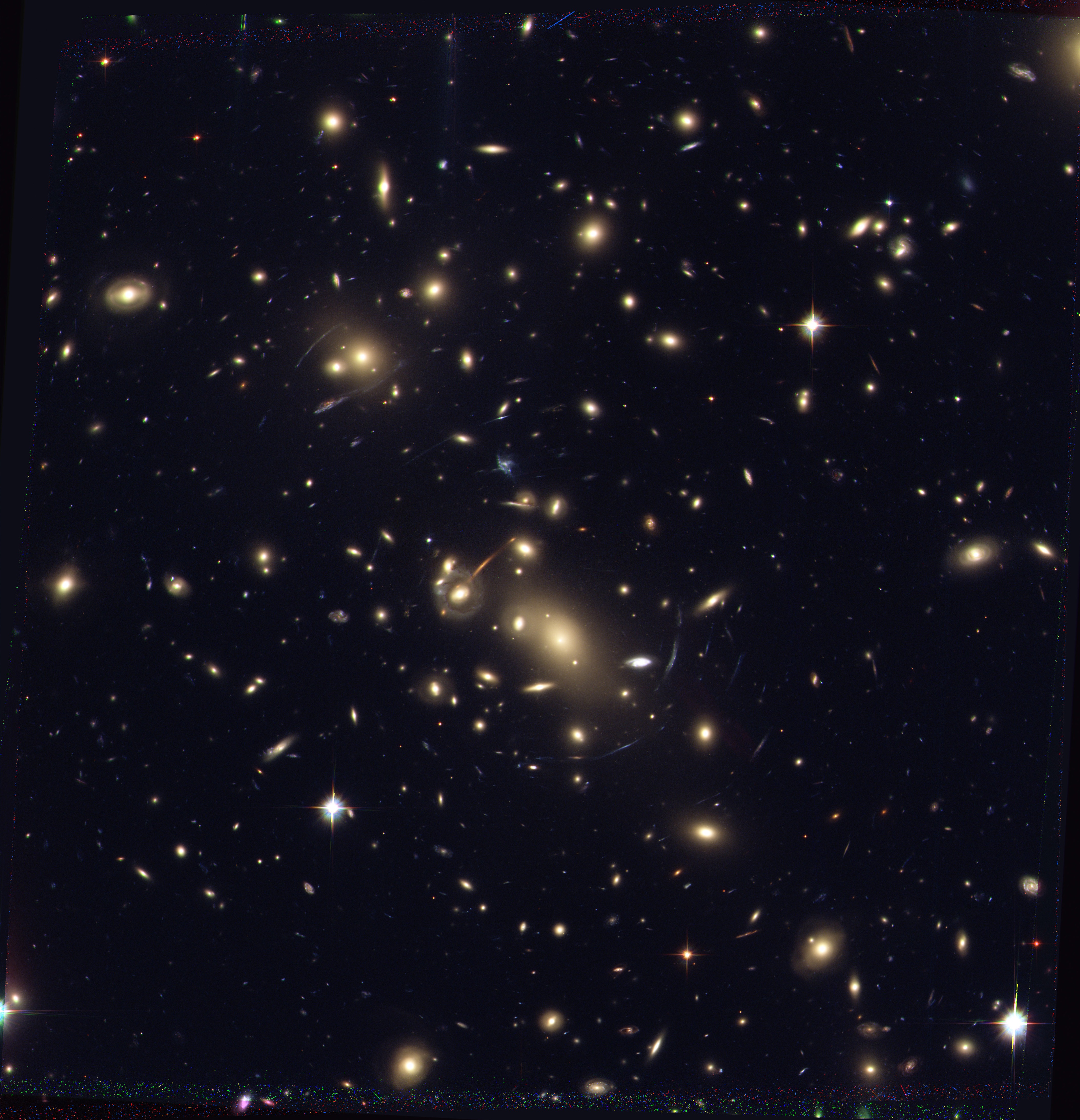
Figure 1: A false color image (B=blue, V=green, z=red) for A2218 from ACS imaging

Detection and photometry were carried out using SEXTRACTOR (Bertin & Arnouts 1996). We used a minimum detection ‘aperture’ of 7 connected pixels $2.0\ \sigma$ above the sky. We also calculated a mean central surface brigthness from a small aperture (of area equivalent to the detection aperture) for star-galaxy separation. We experimented with the parameters to maximize the number of faint objects detections and minimize the number of spurious objects. All detections were examined visually to eliminate noise spikes due to drizzling process, bleed trails from bright stars, arclets (especially !) and false detections. The magnitudes were calibrated to the HST AB system using the published zeropoints on the HST Instrument Web page. We also corrected the magnitudes to SDSS and Johnson-Cousins systems using the values tabulated in Holberg & Bergeron (2006).

We use plots in surface brightness and magnitude space to select a range of luminosities and central surface brightnesses where we are reasonably complete, can separate stars and galaxies and do not suffer excessively from incompleteness at low surface brightness. See Harsono & De Propris (2009) for details.

We can only determine cluster memberships statistically, especially at the faint magnitudes. The ‘field’ galaxies can be removed by observing cluster-less fields. We use the two GOODS fields (Giavalisco et al. 2004) as our reference fields, which have deeper multicolor data. We use the same SExtractor parameters on the GOODS images as the ones used for the clusters. We selected the galaxies in GOODS fields using the limiting magnitudes and surface brightness limits we used for clusters.

The GOODS number counts were fitted with a quadratic fit to smooth out field to field variations in the counts. The reference counts were scaled to the areas surveyed for each cluster and these counts subtracted from the galaxy counts in each cluster field to arrive at an estimate of the luminosity distribution for galaxies in each cluster. Errors include contributions from Poisson shot noise in the cluster, fore/background galaxies in the cluster field and galaxies in the reference field, and clustering errors in the cluster and reference fields, calculated as per Huang et al. (1997) and added in quadrature.

The magnitudes were $k+e$ corrected to $z=0$ for comparison with local data using a Bruzual & Charlot (2003) model for a solar metallicity single stellar population formed at $z=3$ with an e-folding time of 1 Gyr (appropriate for the bright cluster ellipticals). We then calculated composite LFs for each band using the approach in Colless (1989). The LF fits are shown in Figure 2 and are consistent with a single Schechter function: the bottom panels show the associated error ellipse. Table 1 shows the best fit values.

Table 1: Best Schechter Function Fit for Composite LFs

Band	$M_{*}$	$\alpha$	$\chi_{\nu}^{2}$
B (F435W)	$-19.89\pm 0.27$	$-1.29\pm 0.06$	0.59
g (F475W)	$-20.94\pm 0.17$	$-1.31\pm 0.04$	0.95
V (F555W)	$-21.86\pm 0.27$	$-1.27\pm 0.05$	1.08
r (F625W)	$-21.95\pm 0.29$	$-1.33\pm 0.03$	0.43
i (F775W)	$-21.66\pm 0.27$	$-1.27\pm 0.04$	0.37
z (F850LP)	$-22.26\pm 0.30$	$-1.45\pm 0.02$	0.94

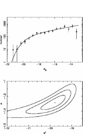
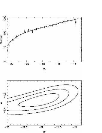
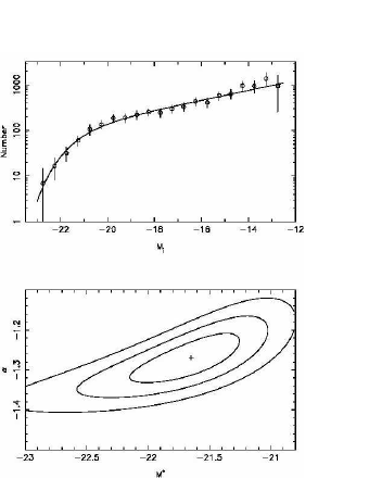
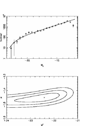
Figure 2: Composite LFs, best fits, and error ellipses for B (top left), r (top right), i (bottom left) and z (bottom right).

3 Evolution of the LF

Our data are consistent with a passively evolving bright-end of the LF, as has been already found out by several studies. The main novel conclusion here regards the evolution of the faint end slope, which is here measured to depths comparable to those reached in the nearby surveys by De Propris et al. (2003) and Popesso et al. (2006). The data show that the LF in these clusters has not evolved significantly since $z=0.3$. This suggests that the entire population of galaxies in these cluster cores (the fields span the inner 1/3 of each cluster) was formed and assembled at least at $z=0.3$ over a luminosity range spanning nearly 3 orders of magnitude.

We also note that the LF slope is the same in all bands. This argues that the cluster population is dominated by galaxies on the red sequence at all luminosities and that there is no evidence for truncation of the red sequence down to $M_{z}=-14$ in these clusters at $z=0.3$ and that the entire red population must have been completely in place by this epoch at least.

We do not detect any sign of an upturn in the LF at faint magnitudes. If this upturn is truly present in local clusters, the data suggest that it may have originated recently, by infall of a very faint field population (Wilson et al. 1997).

We can explore this further by looking at the color-magnitude relation in population sensitive colors. A full analysis of this is deferred to a future paper (Harsono, De Propris & Andreon, in preparation). Here we show (Figure 3) $g-r$ (a color that resembles $U-V$ for the redshifts of our clusters) vs. $z$ (a color that samples more closely the stellar mass of galaxies) for our clusters. We observe that all clusters obey a very tight and linear color magnitude relation, with little evidence of increasing scatter as a function of luminosity (cf., Andreon et al. 2006).

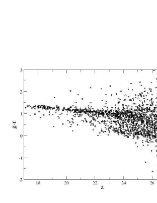
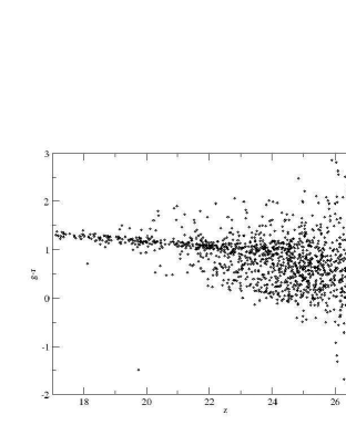
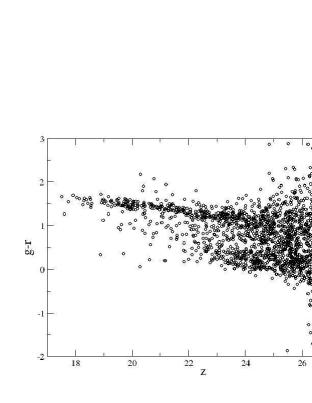
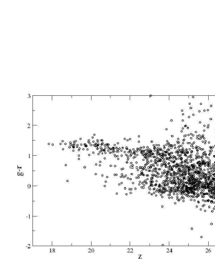
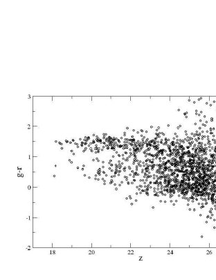
Figure 3: The color magnitude diagrams (CMDs: g-r vs z) for 4 clusters: A1689 (top left), A2218 (top right), A1703 (middle left), MS 1358.4+6245 (middle right) and Cl 0024.0+1652 (bottom left). We arranged CMDs such that the redshift increases from left to right and top to bottom.

We are currently carrying out a rigorous Bayesian analysis to calculate the scatter of the color magnitude relation as a function of luminosity and the red sequence luminosity function. However, if the above result is confirmed, this would suggest that the entire cluster population shared a similar formation history, irrespective of galaxy mass, and that the red sequence was well in place at faint luminosities even at $z>1$ (cf., Bower et al. 1992).

4 Future Work

The limitations of the present study lie principally in the limited number of objects studied and in the fact that the fields found in the archive correspond to the central regions of very massive clusters and therefore constitute a biased sample: progenitor like effects will be most evident in this sample.

We wish to obtain HST data on the cores of poor clusters, chosen as being below the knee of the X-ray luminosity function, with similar depth and band coverage, together with parallel data on the cluster outskirts and, if feasible, a study of the cluster outskirts of our rich cluster targets (analyzed here). This will allow us to study how the LF evolves and depends on environment, and how the color magnitude relation also evolves depending on environment.

An initial analysis of this can be carried out using a few existing archival fields. This is part of our long term study of clusters at intermediate redshifts and will be reported at a future time.

References

- [1] Andreon, S.: 2006, MNRAS, 369, 969
- [2] Andreon, S., Cuillandre, J.-C., Puddu, E. & Mellier, Y.: 2006, MNRAS, 372, 60
- [3] Balogh, M., Eke, V., Miller, C. J., et al.: 2004, MNRAS, 348, 1355
- [4] Barkhouse, W. A., Yee, H. K. C. & Lopez-Cruz, O.: 2007, ApJ, 671, 1471
- [5] Bell, E. F., Naab, T., McIntosh, D. H. et al.: 2006, ApJ, 640, 241
- [6] Bower, R. G., Lucey, J. R. & Ellis, R. S.: 1992, MNRAS, 254, 601
- [7] Bruzual, G. & Charlot, S.: 2003, MNRAS, 344, 1000
- [8] Crawford, S. M., Bershady, M. A. & Hoessel, J. G.: 2009, ApJ, 690, 1158
- [9] De Lucia, G., Poggianti, B. M., Aragon-Salamanca, A. et al: 2007, MNRAS, 374, 809
- [10] De Propris, R., Colless, M. M., Driver, S. P. et al.: 2003, MNRAS, 342, 725
- [11] De Propris, R., Stanford, S. A., Eisenhardt, P. R. et al. 2007, AJ, 133, 2209
- [12] Dressler, A.: 1980, ApJ, 236, 351
- [13] Faber, S. M., Willmer, C. N. A., Wolf, C. et al.: 2007, ApJ, 665, 265
- [14] Giavalisco, M., Ferguson, H. C., Koekemoer, A. M. et al.: 2004, ApJ, 600, L93
- [15] Gomez, P. L., Nichol, R. C., Miller, C. J., et al: 2003, ApJ, 584, 210
- [16] Harsono, D. & De Propris, R.: 2009, AJ, 137, 3109
- [17] Holberg, J. B. & Bergeron, P.: 2006, AJ, 132, 1221
- [18] Khochfar, S., Silk, J., Windhorst, R. A. & Ryan, R. E.: 2007, ApJ, 668, L115
- [19] Koekemoer, A. M., Fruchter, A. S., Hook, R. N. & Hack, W.: 2002, in The 2002 HST Calibration Workshop : Hubble after the Installation of the ACS and the NICMOS Cooling System, ed. S. Arribas, A. Koekemoer, and B. Whitmore (Baltimore: Space Telescope Science Institute), p. 337
- [20] Krick, J. E., Surace, J. A., Thompson, D. et al.: 2008, ApJ, 686, 918
- [21] Lewis, I. J., Balogh, M. L., De Propris, R. et al.: 2002, MNRAS, 334, 673
- [22] Muzzin, A., Wilson, G., Lacy, M. et al.: 2008, ApJ, 686, 966
- [23] Perez-Gonzalez, P. G., Rieke, G. H., Villar, V. et al.: 2008, ApJ, 675, 234
- [24] Popesso, P., Biviano, A., Bohringer, H. & Romaniello, M.: 2006, A&A, 445, 29
- [25] Stott, J. P., Smail, Ian, Edge, A. C. et al.: 2007, ApJ, 661, 95
- [26] Wilson, G., Smail, I., Ellis, R. S. & Couch, W. J.: 1997, MNRAS, 284, 915