On Revenue Maximization in
Second-Price Ad Auctions

Abstract

Most recent papers addressing the algorithmic problem of allocating advertisement space for keywords in sponsored search auctions assume that pricing is done via a first-price auction, which does not realistically model the Generalized Second Price (GSP) auction used in practice. Towards the goal of more realistically modeling these auctions, we introduce the Second-Price Ad Auctions problem, in which bidders’ payments are determined by the GSP mechanism. We show that the complexity of the Second-Price Ad Auctions problem is quite different than that of the more studied First-Price Ad Auctions problem. First, unlike the first-price variant, for which small constant-factor approximations are known, it is NP-hard to approximate the Second-Price Ad Auctions problem to any non-trivial factor. Second, this discrepancy extends even to the $0$-$1$ special case that we call the Second-Price Matching problem (2PM). In particular, offline 2PM is APX-hard, and for online 2PM there is no deterministic algorithm achieving a non-trivial competitive ratio and no randomized algorithm achieving a competitive ratio better than $2$. This stands in contrast to the results for the analogous special case in the first-price model, the standard bipartite matching problem, which is solvable in polynomial time and which has deterministic and randomized online algorithms achieving better competitive ratios. On the positive side, we provide a 2-approximation for offline 2PM and a 5.083-competitive randomized algorithm for online 2PM. The latter result makes use of a new generalization of a classic result on the performance of the “Ranking” algorithm for online bipartite matching.

1 Introduction

The rising economic importance of online sponsored search advertising has led to a great deal of research focused on developing its theoretical underpinnings. (See, e.g., [LPSV07] for a survey). Since search engines such as Google, Yahoo! and Bing depend on sponsored search for a significant fraction of their revenue, a key problem is how to optimally allocate ads to keywords (user searches) so as to maximize search engine revenue [AMT07, AM04, ABK⁺08, BJN07, CG08, DH09, GMNS08, GM08, MNS07, MSVV07, Sri08]. Most of the research on the dynamic version of this problem assumes that once the participants in each keyword auction are determined, the pricing is done via a first-price auction; in other words, bidders pay what they bid. This does not realistically model the standard mechanism used by search engines, called the Generalized Second Price mechanism (GSP) [EOS07, Var07].

In an attempt to model reality more closely, we study the Second-Price Ad Auctions problem, which is the analogue of the above allocation problem when bidders’ payments are determined by the GSP mechanism. As in other work [ABK⁺08, BJN07, CG08, MSVV07, Sri08], we make the simplifying assumption that there is only one slot for each keyword. In this case, the GSP mechanism for a given keyword auction reduces to a second-price auction – given the participants in the auction, it allocates the advertisement slot to the highest bidder, charging that bidder the bid of the second-highest bidder.

In the Second-Price Ad Auctions problem, there is a set of keywords $U$ and a set of bidders $V$, where each bidder $v\in V$ has a known daily budget $B_{v}$ and a non-negative bid $b_{u,v}$ for every keyword $u\in U$. The keywords are ordered by their arrival time, and as each keyword $u$ arrives, the algorithm (i.e., the search engine) must choose a bidder to allocate it to. The search engine is not required to choose the highest-bidding bidder; in order to optimize the allocation of bidders to keywords, search engines typically use a “throttling” algorithm that chooses which bidders to select to participate in an auction for a given keyword [GMNS08].

In the previously-studied first-price version of the problem, allocating a keyword to a bidder meant choosing a single bidder $v$ and allocating $u$ to $v$ at a price of $b_{u,v}$. In the Second-Price Ad Auctions problem, two bidders are selected instead of one. Of these two bidders, the bidder with the higher bid (where bids are always reduced to the minimum of the actual bid and bidders’ remaining budgets) is allocated that keyword’s advertisement slot at the price of the other bid. (In the GSP mechanism for $k$ slots, $k+1$ bidders are selected, and each of the top $k$ bidders pays the bid of the next-highest bidder.)

This process results in an allocation and pricing of the advertisement slots associated with each of the keywords. The goal is to select the bidders participating in each auction to maximize the total profit extracted by the algorithm. For an example instance of this problem, see Figure 1.

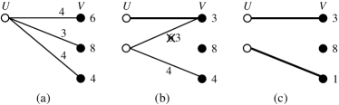
Figure 1: An example of the Second-Price Ad Auctions problem: the nodes in $U$ are keywords and the nodes in $V$ are bidders. The number immediately to the right of each bidder represents its remaining budget, and the number next to each edge connecting a bidder to a keyword represents the bid of that bidder for that keyword. (a) shows the situation when the first keyword arrives. For this keyword, the search engine selects the first bidder, whose bid is 4, and the second bidder, whose bid is 3. The keyword is allocated to the first bidder at a price of 3, thereby reducing that bidder’s budget by 3. (b) shows the situation when the second keyword arrives. The bid of the first bidder for that keyword is adjusted to the minimum of its original bid, $6$, and its remaining budget, $3$. Then the first and the third bidders are selected, and the keyword is allocated to the third bidder at a price of $3$.

1.1 Our Results

We begin by considering the offline version of the Second-Price Ad Auctions problem, in which the algorithm knows all of the original bids of the bidders (Section 3). Our main result here is that it is NP-hard to approximate the optimal solution to this problem to within a factor better than $\Omega(m)$, where $m$ is the number of keywords, even when the bids are small compared to budgets. This strong inapproximability result is matched by the trivial algorithm that selects the single keyword with the highest second-best bidder and allocates only that keyword to its top two bidders. It stands in sharp contrast to the standard First-Price Ad Auctions problem, for which there is a 4/3-approximation to the offline problem [CG08, Sri08] and an $e/(e-1)$-competitive algorithm to the online problem when bids are small compared to budgets [BJN07, MSVV07].

We then turn our attention to a theoretically appealing special case that we call Second-Price Matching. In this version of the problem, all bids are either 0 or 1 and all budgets are 1. This can be thought of as a variant on maximum bipartite matching in which the input is a bipartite graph $G=(U\cup V,E)$, and the vertices in $U$ must be matched, in order, to the vertices in $V$ such that the profit of matching $u\in U$ to $v\in V$ is $1$ if and only if there is at least one additional vertex $v^{\prime}\in V$ that is a neighbor of $u$ and is unmatched at that time. One can justify the second-price version of the problem by observing that when we sell an item, we can only charge the full value of the item when there is more than one interested buyer.

Recall that the first-price analogue to the Second-Price Matching problem, the maximum bipartite matching problem, can be solved optimally in polynomial time. The online version has a trivial 2-competitive deterministic greedy algorithm and an $e/(e-1)$-competitive randomized algorithm due to Karp, Vazirani and Vazirani [KVV90], both of which are best possible.

In contrast, we show that the Second-Price Matching problem is APX-hard (Section 4.1). We also give a 2-approximation algorithm for the offline problem (Section 4.2). We then turn to the online version of the problem. Here, we show that no deterministic online algorithm can get a competitive ratio better than $m$, where $m$ is the number of keywords in the instance, and that no randomized online algorithm can get a competitive ratio better than 2 (Section 5.1). On the other hand, we present a randomized online algorithm that achieves a competitive ratio of $2\sqrt{e}/(\sqrt{e}-1)\approx 5.08$ (Section 5.2). To obtain this competitive ratio, we prove a generalization of the result due to Karp, Vazirani, and Vazirani [KVV90] and Goel and Mehta [GM08] that the Ranking algorithm for online bipartite matching achieves a competitive ratio of $e/(e-1)$.

	Offline		Online
	Upper bound	Lower bound	Upper bound	Lower bound
1PAA	$4/3$ [CG08, Sri08]	$16/15$ [CG08]	$e/(e-1)^{*}$ [BJN07, MSVV07] or $2$ [LLN06]	$e/(e-1)$ [MSVV07, KVV90]
2PAA	$O(m)$	$\Omega(m)$	-	-
Matching	poly-time alg.		$e/(e-1)$ [KVV90, GM08]	$e/(e-1)$ [KVV90]
2PM	$2$	$364/363$	$2\sqrt{e}/(\sqrt{e}-1)\approx 5.083$	$2$

Table 1: A summary of the results in this paper, compared to known results for the first-price case. The upper bound of $e/(e-1)$ for Online 1PAA only holds when when the bids are small compared to the budgets.

1.2 Related Work

As discussed above, the related First-Price Ad Auctions problem has received a fair amount of attention. Mehta et al. [MSVV07] present an algorithm for the online version that achieves an optimal competitive ratio of $e/(e-1)$ for the case when the bids are much smaller than the budgets, a result also proved by Buchbinder et al. [BJN07]. Under similar assumptions, Devanur and Hayes show that when the keywords arrive according to a random permutation, a $(1-\varepsilon)$-approximation is possible [DH09]. When there is no restriction on the values of the bids relative to the budgets, the best known competitive ratio is 2 [LLN06]. For the offline version of the problem, a sequence of papers [LLN06, AM04, FV06, ABK⁺08, Sri08, CG08] culminating in a paper by Chakrabarty and Goel, and independently, a paper by Srinivasan, show that the offline problem can be approximated to within a factor of $4/3$ and that there is no polynomial time approximation algorithm that achieves a ratio better than 16/15 unless $P=NP$ [CG08].

The most closely related work to ours is the paper of Goel, Mahdian, Nazerzadeh and Saberi [GMNS08], which builds on the work of Abrams, Medelvitch, and Tomlin [AMT07]. Goel et al. look at the online allocation problem when the search engine is committed to charging under the GSP scheme, with multiple slots per keyword. They study two models, the “strict” and “non-strict” models, both of which differ from our model even for the one slot case by allowing bidders to keep bidding their orginal bid, even when their budget falls below this amount. Thus, in these models, although bidders are not charged more than their remaining budget when allocated a keyword, a bidder with a negligible amount of remaining budget can keep his bids high indefinitely, and as long as this bidder is never allocated another slot, this high bid can determine the prices other bidders pay on many keywords. Under the assumption that bids are small compared to budgets, Goel et al. build on the linear programming formulation of Abrams et al. to present an $e/(e-1)$-competitive algorithm for the non-strict model and a 3-competitive algorithm for the strict model.

The significant, qualitative difference between these positive results and the strong hardness we prove for our model suggests that these aspects of the problem formulation are important. We feel that our model, in which bidders are not allowed to bid more than their remaining budget, is more natural because it seems inherently unfair that a bidder with negligible or no budget should be able to indefinitely set high prices for other bidders.

2 Model and Notation

We define the Second-Price Ad Auctions (2PAA) problem formally as follows. The input is a set of ordered keywords $U$ and bidders $V$. Each bidder $v\in V$ has a budget $B_{v}$ and a nonnegative bid $b_{u,v}$ for every keyword $u\in U$. We assume that all of bidder $v$’s bids $b_{u,v}$ are less than or equal to $B_{v}$.

Let $B_{v}(t)$ be the remaining budget of bidder $v$ immediately after the $t$-th keyword is processed (so $B_{v}(0)=B_{v}$ for all $v$), and let $b_{u,v}(t)=\min(b_{u,v},B_{v}(t))$. (Both quantities are defined inductively.) A solution (or second-price matching) to 2PAA chooses for the $t$-th keyword $u$ a pair of bidders $v_{1}$ and $v_{2}$ such that $b_{u,v_{1}}(t-1)\geq b_{u,v_{2}}(t-1)$, allocates the slot for keyword $u$ to bidder $v_{1}$ and charges bidder $v_{1}$ a price of $p(t)=b_{u,v_{2}}(t-1)$, the bid of $v_{2}$. (We say that $v_{1}$ acts as the first-price bidder for $u$ and $v_{2}$ acts as the second-price bidder for $u$.) The budget of $v_{1}$ is then reduced by $p(t)$, so $B_{v_{1}}(t)=B_{v_{1}}(t-1)-p(t)$. For all other bidders $v\neq v_{1}$, $B_{v}(t)=B_{v}(t-1)$. The final value of the solution is $\sum_{t}p(t)$, and the goal is to find a solution of maximum value.

In the offline version of the problem, all of the bids are known to the algorithm beforehand, whereas in the online version of the problem, keyword $u$ and the bids $b_{u,v}$ for each $v\in V$ are revealed only when keyword $u$ arrives, at which point the algorithm must irrevocably map $u$ to a pair of bidders without knowing the bids for the keywords that will arrive later.

The special case referred to as Second-Price Matching (2PM) is where $b_{u,v}$ is either 0 or 1 for all $(u,v)$ pairs and $B_{v}=1$ for all $v$. We will think of this as the variant on maximum bipartite matching (with input $G=(U\cup V,E)$) described in Section 1.1. Note that in 2PM, a keyword can only be allocated for profit if its degree is at least two. Therefore, we assume without loss of generality that for all inputs of 2PM, the degree of every keyword is at least two.

For an input to 2PAA, let $R_{min}=\min_{u,v}B_{v}/b_{u,v}$, and let $m=|U|$ be the number of keywords.

3 Hardness of Approximation of 2PAA

In this section, we present our main hardness result for the Second-Price Ad Auctions problem. For a constant $c\geq 1$, let 2PAA($c$) be the version of 2PAA in which we are promised that $R_{min}\geq c$.

Theorem 1.

Let $c\geq 1$ be a constant integer. For any constant $c^{\prime}>c$, it is NP-hard to approximate 2PAA($c$) to a factor of $m/c^{\prime}$.

Hence, even when the bids are guaranteed to be smaller than the budget by a large constant factor, it is NP-hard to approximate 2PAA to a factor better than $\Omega(m)$. After proving this result, we show in Theorem 2 that this hardness is matched by a trivial algorithm.

Proof.

Fix a constant $c^{\prime}>c$, and let $n_{0}$ be the smallest integer such that for all $n\geq n_{0}$,

$$c^{\prime}\cdot\frac{c(n^{5}+n+2)}{cn^{2}+n+2}\geq c(n^{3}+cn^{2}+n+2)$$ (1)

and

$$\frac{n/2+1}{2}\geq c\enspace.$$ (2)

Note that since $n_{0}$ depends only on $c^{\prime}$, it is a constant.

We reduce from PARTITION, in which the input is a set of $n\geq n_{0}$ items, and the weight of the $i$-th item is given by $w_{i}$. If $W=\sum_{i=1}^{n}w_{i}$, then the question is whether there is a partition of the items into two subsets of size $n/2$ such that the sum of the $w_{i}$’s in each subset is $W/2$. It is known that this problem (even when the subsets must both have size $n/2$) is NP-hard [GJ79].

Given an instance of PARTITION, we create an instance of 2PAA($c$) as follows. (This reduction is illustrated in Figure 2.)

• First, create $n+2$ keywords $c_{1},\ldots,c_{n},e_{1},e_{2}$. Second, create an additional set

  $$G=\left\{{g_{i,k}\mbox{ }:\mbox{ }1\leq i\leq n^{2}\mbox{ and }1\leq k\leq c}\right\}$$

  of $cn^{2}$ keywords. The keywords arrive in the order

  $$c_{1},\ldots,c_{n},e_{1},e_{2},g_{1,1},\ldots,g_{1,c},\ldots\ldots,g_{n^{2},1},\ldots,g_{n^{2},c}\enspace.$$

• Create $n^{2}+4$ bidders $a,d_{1},d_{2},f,h_{1},\ldots,h_{n^{2}}$. Set the budgets of $a$, $d_{1}$, and $d_{2}$ to $cW(1+n/2)$. Set the budget of $f$ to $cW(n^{3}+1)$. For $1\leq i\leq n^{2}$, set the budget of $h_{i}$ to $cWn^{3}$.

• For $1\leq i\leq n$, bidders $a$, $d_{1}$, and $d_{2}$ bid $c(w_{i}+W)$ on keyword $c_{i}$.

• For $j\in\left\{{1,2}\right\}$, bidder $d_{j}$ bids $cW$ on keyword $e_{j}$. Bidder $f$ bids $cW/2$ on both $e_{1}$ and $e_{2}$.

• For $1\leq i\leq n^{2}$ and $1\leq k\leq c$, keyword $g_{i,k}$ receives a bid of $W(n^{3}+1)$ from bidder $f$ and a bid of $Wn^{3}$ from bidder $h_{i}$.

This reduction can clearly be performed in polynomial time. Furthermore, it can easily be checked that (2) implies that no bidder bids more than $1/c$ of its budget on any keyword.

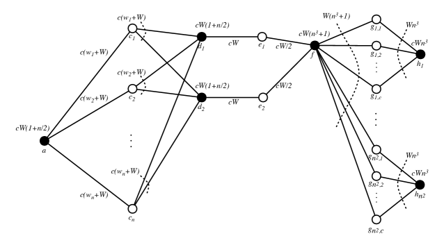
Figure 2: The 2PAA($c$) instance of the reduction. Each bidder’s budget is shown above its node, and the bids of bidders for keywords is shown near the corresponding edge.

We first show that if the PARTITION instance is a “yes” instance, then there exists a feasible solution to the 2PAA($c$) instance of value at least $cW(n^{5}+n+2)$. Let $S\subseteq\left[{n}\right]$ be such that $|S|=n/2$ and $\sum_{i\in S}w_{i}=\sum_{i\in\overline{S}}w_{i}=W/2$. We construct a solution to the 2PAA($c$) instance as follows. For every $i\in S$, allocate $c_{i}$ to $d_{1}$, and for every $i\in\overline{S}$, allocate $c_{i}$ to $d_{2}$. For each of these allocations, choose $a$ as the second-price bidder. This will reduce the budget of $d_{1}$ and $d_{2}$ to exactly $cW/2$, and hence the bids from $d_{1}$ to $e_{1}$ and from $d_{2}$ to $e_{2}$ will both be reduced to $cW/2$. Allocate $e_{1}$ to $f$ choosing $d_{1}$ as the second-price bidder, and allocate $e_{2}$ to $f$ choosing $d_{2}$ as the second-price bidder. This will reduce the budget of $f$ to $cWn^{3}$. The profit from the solution constructed so far is $cW(n+2)$. Now allocate $g_{1,1},g_{1,2},\ldots,g_{1,c-1}$ to $f$, choosing $h_{1}$ as the second-price bidder. This will reduce the budget of $f$ to $Wn^{3}$. Hence, it can act as the second-price bidder for each of the remaining keywords in $G$. Allocate $g_{1,c}$ to $h_{1}$, choosing $f$ as the second-price bidder, and then, for $2\leq i\leq n^{2}$ and $1\leq k\leq c$, allocate $g_{i,k}$ to $h_{i}$, choosing $f$ as the second-price bidder. The profit obtained for each keyword in $G$ in this assignment is $Wn^{3}$. Since $|G|=cn^{2}$, the total profit of the solution constructed is $cW(n+2)+cWn^{5}=cW(n^{5}+n+2)$.

We now show that if there is a second-price matching in the 2PAA($c$) instance of value at least $cW(n^{3}+cn^{2}+n+2)$, then there must be a partition of $w_{1},\ldots,w_{n}$. In such a matching, at most $cW(n+2)$ units of profit can be obtained from keywords $c_{1},\ldots,c_{n},e_{1},e_{2}$, since the initial second-highest bids on those keywords sum to $cW(n+2)$. Hence, at least $cW(n^{3}+cn^{2})$ profit must come from the keywords in $G$.

Suppose that the budget of $f$ is greater than $cWn^{3}$ after keywords $e_{1}$ and $e_{2}$ are allocated. Note that at least $c$ of the keywords in $G$ must be allocated to reach a profit of $cW(n^{3}+cn^{2})$ on these keywords. Consider what happens after the first $c$ of the keywords in $G$ are assigned. For each of these keywords, $f$ must have been the first-price bidder, so its budget is reduced to an amount greater than $0$ and less than or equal to $cW$. Hence, for each keyword in $G$ allocated henceforth, $f$ is the second-price bidder, and the profit is at most $cW$. Since there are at most $c(n^{2}-1)$ more keywords in $G$, the total profit from the keywords in $G$ is at most $cWn^{3}+c^{2}W(n^{2}-1)$, which contradicts the fact that at least $cW(n^{3}+cn^{2})$ units of profit must come from $G$. Hence, we conclude that the budget of $f$ is less than or equal to $cWn^{3}$ after keywords $e_{1}$ and $e_{2}$ are allocated.

The budget of $f$ can only be smaller than $cWn^{3}$ if $f$ acts as the first-price bidder for both $e_{1}$ and $e_{2}$. But this can happen only if the budgets of both $d_{1}$ and $d_{2}$ are reduced to an amount less than or equal to $cW/2$. For $j\in\left\{{1,2}\right\}$, let $S_{j}\subseteq\left[{n}\right]$ be the set of indices $i$ such that $d_{j}$ acts as the first-price bidder for $i$. For both $j$, we have that

$$\sum_{i\in S_{j}}c(w_{i}+W)\geq\frac{cW}{2}+\frac{cWn}{2}\enspace.$$ (3)

Rearranging (3) yields $\sum_{i\in S_{j}}W\geq W/2+Wn/2-\sum_{i\in S_{j}}w_{i}$, which implies $W|S_{j}|\geq W/2+Wn/2-W$, and hence $|S_{j}|\geq n/2-1/2$. By integrality, then, $|S_{j}|\geq n/2$ for both $j$. Hence $|S_{j}|=n/2$ for both $j$, and using (3) again, we have $\sum_{i\in S_{j}}cw_{i}+cW|S_{j}|\geq cW/2+cWn/2$ which implies that $\sum_{i\in S_{j}}w_{i}\geq W/2$ for both $j$. Therefore, the partition defined by $S_{1}$ and $S_{2}$ is a solution to the PARTITION instance.

To conclude the proof, note that there are $cn^{2}+n+2$ keywords in the 2PAA($c$) instance. Hence, if the PARTITION instance is a “yes” instance, then by (1), we can run an $m/c^{\prime}$-approximation algorithm to find a second-price matching of value at least $cW(n^{3}+cn^{2}+n+2)$, and if the PARTITION instance is a “no” instance, then the value of the solution returned by such an algorithm must be strictly less than $cW(n^{3}+cn^{2}+n+2)$. Hence, an $m/c^{\prime}$-approximation algorithm for 2PAA($c$) can be used to solve PARTITION. ∎

Theorem 2.

Let $c\geq 1$ be a constant integer. There is an $m/c$-approximation to 2PAA($c$).

Proof.

For each keyword $u\in U$, let $s_{u}$ be the second-highest bid for $u$. Consider the algorithm that selects the $c$ keywords with the highest values of $s_{u}$ and then allocates these keywords to get $s_{u}$ for each of them (i.e., chooses the two highest bidders for $u$). Since no bidder bids more than $1/c$ of its budget for any keyword, no bids are reduced from their original values during this allocation. Hence, the profit of this allocation is at least $(c/m)\sum_{u\in U}s_{u}$. Since the value of the optimal solution cannot be larger than $\sum_{u\in U}s_{u}$, it follows that this is an $m/c$-approximation to 2PAA($c$). ∎

4 Offline Second-Price Matching

In this section, we turn our attention to the offline version of the special case of Second-Price Matching (2PM). Before we show our bounds on the approximability of 2PM, we start with a simple proof that it is NP-hard. Then, in Section 4.1, we show that 2PM is APX-hard, and in Section 4.2, we give a 2-approximation for 2PM.

Theorem 3.

The Second-Price Matching Problem is NP-hard.

Note that this result is subsumed by Theorem 5 below. We present it anyway because it allows us to illustrate a simpler reduction to the problem.

Proof.

We reduce from 3-SAT. Given an instance of 3-SAT in which the variables are $X=\left\{{x_{1},\ldots,x_{n}}\right\}$ and the clauses are $\mathcal{C}=\left\{{c_{1},\ldots,c_{k}}\right\}$, we construct an instance of 2PM as follows:

• For each variable $x_{i}\in X$, there is a keyword $v_{i}$. We call these keywords the variable keywords. Each variable keyword $v_{i}$ is connected to two bidders $v_{i}^{t}$ and $v_{i}^{f}$. We call these bidders the assignment bidders.

• For each clause $c_{j}\in\mathcal{C}$, there is a keyword $u_{j}$ and a bidder $b_{j}$. We call these keywords and bidders clause keywords and clause bidders, respectively. Each clause keyword $u_{j}$ is connected to $b_{j}$ and three of the assignment bidders, one for each literal $\ell\in c_{j}$, chosen as follows. If $\ell$ is of the form $x_{i}$ for some variable $x_{i}$, then $u_{j}$ is connected to $v_{i}^{f}$. Otherwise, if $\ell$ is of the form $\overline{x_{i}}$ for some variable $x_{i}$, then $u_{j}$ is connected to $v_{i}^{t}$.

The keywords arrive in two phases: first the variable keywords and then the clause keywords. An example of this reduction is illustrated in Figure 3.

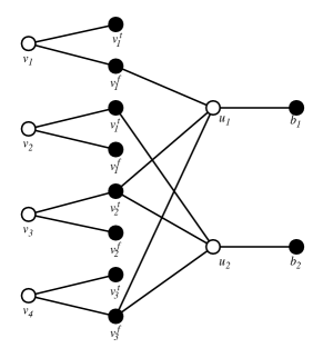
Figure 3: An example of the reduction from 3-SAT to 2PM. The formula represented is $(x_{1}\vee\overline{x_{3}}\vee x_{4})\wedge(\overline{x_{2}}\vee\overline{x_{3}}\vee x_{4})$.

We now show that the 2PM instance has a second-price matching of value $k+n$ if and only if there is a satisfying assignment to the 3-SAT instance. Suppose first that there is a satisfying assignment to the 3-SAT instance. Let $h:X\rightarrow\left\{{t,f}\right\}$ be the satisfying assignment. We construct a second-price matching as follows. During the first phase, assign each variable keyword $v_{i}$ to $v_{i}^{h(x_{i})}$. The profit from this phase is $n$. During the second phase, assign each clause keyword $u_{j}$ to $b_{j}$. Since $c_{j}$ has at least one satisfied literal $\ell$, the assignment bidder corresponding to $\ell$ will not have been used in the first phase, and the profit for assigning $u_{j}$ to $b_{j}$ is $1$. Thus, the total profit from this phase is $k$, and the total profit of the second-price matching is $k+n$.

On the other hand, if there is a second-price matching of size at least $k+n$, then since there are $k+n$ keywords in the 2PMM instance, the profit obtained from each keyword in the second-price matching must be $1$. This means that each variable keyword must have been matched to one of its assignment bidders during the first phase. Let $h:X\rightarrow\left\{{t,f}\right\}$ be the assignment generated from this matching, i.e., if $v_{i}$ was assigned to $v_{i}^{\ell}$ (for $\ell\in\left\{{t,f}\right\}$), then let $h(x_{i})=\ell$. Since the profit obtained from each keyword is $1$, each clause keyword $u_{j}$ must have been adjacent to at least two unused bidders when it was assigned, including one of the assignment bidders, say $v_{i}^{\ell}$. Hence, $h(x_{i})=\overline{\ell}$, and by construction of the 2PMM instance, clause $c_{j}$ is satisfied by $h$. We conclude that $h$ is a satisfying assignment to the 3-SAT instance. ∎

4.1 Hardness of Approximation

To prove that 2PM is APX-hard, we reduce from vertex cover, using the following result.

Theorem 4 (Chlebík and Chlebíková [CC06]).

It is NP-hard to approximate Vertex Cover on 4-regular graphs to within $53/52$.

The precise statement of our hardness result is the following theorem.

Theorem 5.

It is NP-hard to approximate 2PM to within a factor of $364/363$.

Proof.

Given a graph $G$ as input to Vertex Cover, we construct an instance $f(G)$ of 2PM as follows. First, for each edge $e\in E(G)$, we create a keyword with the same label (called an edge keyword), and for each vertex $v\in V(G)$, we create a bidder with the same label (called a vertex bidder). Bidder $v$ bids for keyword $e$ if vertex $v$ is one of the two end points of edge $e$. (Recall that in 2PM, if a bidder makes a non-zero bid for a keyword, that bid is $1$.) In addition, for each edge $e$, we create a unique bidder $x_{e}$ who also bids for $e$. Furthermore, for each vertex $v$, we create a gadget containing two keywords $h_{v}$ and $l_{v}$ and two bidders $y_{v}$ and $z_{v}$. We let $v$ and $y_{v}$ bid for $h_{v}$; and $y_{v}$ and $z_{v}$ bid for $l_{v}$. The keywords arrive in an order such that for each $v\in V(G)$, keyword $h_{v}$ comes before $l_{v}$, and the edge keywords arrive after all of the $h_{v}$’s and $l_{v}$’s have arrived. An example of this reduction is shown in Figure 4.

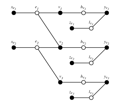
Figure 4: The reduction from an instance $G$ of vertex cover (Figure 4) to an instance $f(G)$ of 2PM (Figure 4).

The following lemma provides the basis of the proof.

Lemma 6.

Let $OPT_{VC}$ and $OPT_{2P}$ be the size of the minimum vertex cover of $G$ and the maximum second-price matching on $f(G)$, respectively. Then

$$OPT_{2P}=2|V(G)|+|E(G)|-OPT_{VC}$$

Proof.

We first show that given a vertex cover $S$ of size $OPT_{VC}$ of $G$, we can construct a solution to the 2PM instance whose value is $2|V(G)|+|E(G)|-OPT_{VC}$. For each vertex $v\notin S$, we allocate $h_{v}$ to $v$ (with $y_{v}$ acting as the second-price bidder) and $l_{v}$ to $y_{v}$ (with $z_{v}$ acting as the second-price bidder), getting a profit of $2$ from the gadget for $v$. For each vertex $v\in S$, we allocate $h_{v}$ to $y_{v}$ (with $v$ acting as the second-price bidder) and ignore $l_{v}$, getting a profit of $1$ from the gadget for $v$. We then allocate each edge keyword $e$ to $x_{e}$. During each of these edge keyword allocations, at least one of the two vertex bidders that bid for $e$ is still available, since $S$ is a vertex cover. Hence, for each of these allocations, there is a bidder that can act as a second-price bidder, and the profit from the allocation is $1$. This allocation yields a second-price matching of size $2|V(G)|+|E(G)|-OPT_{VC}$. Therefore, $OPT_{2P}\geq 2|V(G)|+|E(G)|-OPT_{VC}$.

To show that $OPT_{2P}\leq 2|V(G)|+|E(G)|-OPT_{VC}$, we start with an optimal solution to $f(G)$ of value $OPT_{2P}$ and construct a vertex cover of $G$ of size $2|V(G)|+|E(G)|-OPT_{2P}$. To do this, we first claim that there exists an optimal solution of $f(G)$ in which every edge-keyword is allocated for a profit of $1$. Consider any optimal second-price matching of the instance. Let $e$ be an edge-keyword $e$ that is not allocated for a profit of $1$. If it is adjacent to a vertex bidder that is unassigned when $e$ arrives, then $e$ can be allocated to $x_{e}$ for a profit of $1$, which can only increase the value of the solution. Suppose, on the other hand, that both of its vertex bidders are not available when $e$ arrives. Let $v$ be a vertex bidder that bids for $e$. Since it is not available, $h_{v}$ must have been allocated to $v$. We can transform this second-price matching to another one in which $h_{v}$ is assigned to $y_{v}$, $l_{v}$ is ignored and $e$ is assigned to $x_{e}$, with $v$ acting the second-price bidder in both cases. This does not decrease the total profit of the solution. Hence, we can perform these transformations for each edge keyword $e$ that is not allocated for a profit of $1$ until we obtain a new optimal solution in which each edge keyword is allocated for a profit of $1$.

Now consider an optimal second-price matching in which all edge keywords are allocated for a profit of $1$. Let $T\subseteq V(G)$ be the set of vertices represented by vertex bidders that are not allocated any keywords in this second-price matching. Then $|T|=2|V(G)|+|E(G)|-|OPT_{2P}|$, and $T$ is a vertex cover, which implies $OPT_{VC}\leq 2|V(G)|+|E(G)|-OPT_{2P}$. The lemma follows. ∎

Now, suppose that we have an $\alpha$-approximation for 2PM. We will show how to use this approximation algorithm and our reduction to obtain an $((8\alpha-7)/\alpha)$-approximation for Vertex Cover on 4-regular graphs. By Theorem 4, this means that $(8\alpha-7)/\alpha\geq 53/52$, and hence $\alpha\geq 364/363$, unless $P=NP$.

To construct this $((8\alpha-7)/\alpha)$-approximation algorithm, given a 4-regular graph $G$, run the above reduction to obtain a 2PM instance $f(G)$. Then use the $\alpha$-approximation to obtain a second-price matching $M$ whose value is at least $OPT_{2P}/\alpha$. Now, just as in the proof of Lemma 6, we can assume that in $M$, every edge keyword $e$ is allocated to $x_{e}$. Hence, the set of vertices $T$ associated with the vertex bidders that are not allocated a keyword form a vertex cover, and

$$|T| \leq 2|V(G)|+|E(G)|-OPT_{2P}/\alpha$$ (4)

$$= 2|V(G)|+|E(G)|-(2|V(G)|+|E(G)|-OPT_{VC})/\alpha$$

$$= (1-1/\alpha)(2|V(G)|+|E(G)|)+OPT_{VC}/\alpha$$

Since $G$ is $4$-regular, we have $OPT_{VC}\geq m/4=(2|V(G)|+|E(G)|)/8$, and hence by (4), we conclude that $|T|\leq((8\alpha-7)/\alpha)OPT_{VC}$, which finishes the proof of the theorem. ∎

4.2 A 2-Approximation Algorithm

Consider an instance $G=(U\cup V,E)$ of the 2PM problem. We provide an algorithm that first finds a maximum matching $f:U\rightarrow V$ and then uses $f$ to return a second-price matching that contains at least half of the keywords matched by $f$. Given a matching $f$, call an edge $(u,v)\in E$ such that $f(u)\not=v$ an up-edge if $v$ is matched by $f$ and $f^{-1}(v)$ arrives before $u$, and a down-edge otherwise. Recall that we have assumed without loss of generality that the degree of every keyword in $U$ is at least two. Therefore, every keyword $u\in U$ that is matched by $f$ must have at least one up-edge or down-edge. Theorem 7 shows that the following algorithm, called ReverseMatch, is a $2$-approximation for 2PM.

ReverseMatch Algorithm: Initialization: Find an arbitrary maximum matching $f:U\rightarrow V$ on $G$. Constructing a 2nd-price matching: Consider the matched keywords in reverse order of their arrival. For each keyword $u$:         If keyword $u$ is adjacent to a down-edge $(u,v)$:              Assign keyword $u$ to bidder $f(u)$ (with $v$ acting as the second-price bidder).         Else:              Choose an arbitrary bidder $v$ that is adjacent to keyword $u$.              Remove the edge $(f^{-1}(v),v)$ from $f$.              Assign keyword $u$ to bidder $f(u)$ (with $v$ acting as the second-price bidder).

Theorem 7.

The ReverseMatch algorithm is a 2-approximation.

Proof.

Since the number of vertices matched by $f$ is an upper bound on the profit of the maximum second-price matching on $G$, we need only to prove that the second-price matching contains at least half of the keywords matched by $f$. By the behavior of the algorithm, it is clear that whenever a vertex $u$ is matched to $f(u)$ in the second-price matching, the profit obtained is $1$. Furthermore, every time an an edge is removed from $f$, a new keyword is added to the second-price matching. Thus, the theorem follows. ∎

5 Online Second-Price Matching

In this section, we consider the online 2PM problem, in which the keywords arrive one-by-one and must be matched by the algorithm as they arrive. We start, in Section 5.1, by giving a simple lower bound showing that no deterministic algorithm can achieve a competitive ratio better than $m$, the number of keywords. Then we move to randomized online algorithms and show that no randomized algorithm can achieve a competitive ratio better than $2$. In Section 5.2, we provide a randomized online algorithm that achieves a competitive ratio of $2\sqrt{e}/(\sqrt{e}-1)\approx 5.083$.

5.1 Lower Bounds

The following theorem establishes our lower bound on deterministic algorithms, which matches the trivial algorithm of arbitrarily allocating the first keyword to arrive, and refusing to allocate any of the remaining keywords.

Theorem 8.

For any $m$, there is an adversary that creates a graph with $m$ keywords that forces any deterministic algorithm to get a competitive ratio no better than $m$.

Proof.

The adversary shows the algorithm a single keyword (keyword $1$) that has two adjacent bidders, $a_{1}$ and $b_{2}$. If the algorithm does not match keyword $1$ at all, a new keyword $2$ arrives that is adjacent to two new bidders $a_{2}$ and $b_{2}$. The adversary continues in this way until either $m$ keywords arrive or the algorithm matches a keyword $k<m$. In the first case, the algorithm’s performance is at most $1$ (because it might match keyword $m$), whereas the adversary can match all $m$ keywords. Hence, the ratio is at least $m$.

In the second case, the adversary continues as follows. Suppose without loss of generality that the algorithm matches keyword $k$ to $a_{k}$. Then each keyword $i$, for $k+1\leq i\leq m$, has one edge to $a_{k}$ and one edge to a new bidder $c_{i}$. Since the algorithm cannot match any of these keywords for a profit, its performance is $1$. The adversary can clearly match each keyword $i$ for profit, for $1\leq i\leq k-1$, and if it matches keyword $k$ to $b_{k}$, then it can use $a_{k}$ as a second-price bidder for the remaining keywords to match them all to the $c_{i}$’s for profit. Hence, the adversary can construct a second-price matching of size at least $m$. ∎

We next show that no online (randomized) online algorithm for 2PM can achieve a competitive ratio better than $2$.

Theorem 9.

The competitive ratio of any randomized algorithm for 2PM must be at least $2$.

Proof.

We invoke Yao’s Principle [Yao77] and construct a distribution of inputs for which the best deterministic algorithm achieves an expected performance of (asymptotically) $1/2$ the value of the optimal solution.

Our distribution is constructed as follows. The first keyword arrives, and it is adjacent to two bidders. Then the second keyword arrives, and it is adjacent to one of the two bidders adjacent to the first keyword, chosen uniformly at random, as well as a new bidder; then the third keyword arrives, and it is adjacent to one of the bidders adjacent to the second keyword, chosen uniformly at random, as well as a new bidder; and so on, until the $m$-th keyword arrives. We call this a normal instance. To analyze the performance of the online algorithms, we also define a restricted instance to be one that is exactly the same as a normal instance except that one of the two bidders of the first keyword is marked unavailable, i.e., he can not participate in any auction.

Clearly, an offline algorithm that knows the random choices beforehand can allocate each keyword to the bidder that will not be adjacent to the keyword that arrives next. In this way, it can ensure that for each keyword, there is a bidder that can act as a second-price bidder. Hence for a normal instance, the optimal second-price matching obtains a profit of $m$.

Consider the algorithm Greedy, which allocates a keyword to an arbitrary adjacent bidder if and only if there is another available bidder to act as a second-price bidder. Our proof consists of two steps: first, we will show that the expected performance of Greedy on the normal instance is $(m+1)/2$, and second we will prove that Greedy is the best algorithm in expectation for both types of instances.

Let $X_{k}^{*}$ and $Y_{k}^{*}$ be the expected profit of Greedy on a normal and a restricted instance of $k$ keywords, respectively (where $X_{0}^{*}$ and $Y_{0}^{*}$ are both defined to be $0$). Given the first keyword of a normal instance, Greedy allocates it to an arbitrary bidder. Then, with probability $1/2$, it is faced with a normal instance of $k-1$ keywords, and with probability $1/2$, it is faced with a restricted instance of $k-1$ keywords. Therefore, for all integers $k\geq 1$,

$$X_{k}^{*}=1/2(X_{k-1}^{*}+Y_{k-1}^{*})+1\enspace.$$ (5)

On the other hand, given the first keyword of a restricted instance, Greedy just waits for the second keyword. Then, with probability $1/2$, the second keyword chooses the marked bidder, giving Greedy a restricted instance of $k-1$ keywords, and with probability $1/2$, the second keyword chooses the unmarked bidder, giving Greedy a normal instance of $k-1$ keywords. Therefore, for all $k$,

$$Y_{k}^{*}=1/2(X^{*}_{k-1}+Y^{*}_{k-1})\enspace.$$ (6)

From (5) and (6) we have, for all $k$,

$$Y_{k}^{*}=X_{k}^{*}-1\enspace.$$ (7)

Plugging (7) for $k=m-1$ into (5) for $k=m$ yields

$$X_{m}^{*}=X_{m-1}^{*}+1/2\enspace,$$ (8)

and hence, by induction $X_{m}^{*}=(m+1)/2$.

Now, we prove that Greedy is the best among all algorithms on these two types of instances. In fact, we make it easier for the algorithms by telling them beforehand how many keywords in the instance they will need to solve. Let $X_{m}$ and $Y_{m}$ be the expected number of keywords in the second-price matching produced by the best algorithms that “know” that they are solving a normal instance of size $m$ and a restricted instance of size $m$, respectively. Let ${\cal A}_{m}$ and ${\cal B}_{m}$ denote these optimal algorithms.

We prove that $X_{m}\leq X_{m}^{*}$ and $Y_{m}\leq Y_{m}^{*}$ for all $m$ by induction. The base case in which $m=1$ is easy, since no algorithm can obtain a profit of more than one on a normal instance of one keyword or more than zero on a restricted instance of one keyword. We now prove the induction step.

First, consider ${\cal A}_{m}$. When the first keyword arrives, ${\cal A}_{m}$ has two choices: either ignore it or allocate it to one of the bidders. If ${\cal A}_{m}$ ignores the first keyword, its performance is at most the performance of ${\cal A}_{m-1}$ on the remaining keywords, which constitute a normal instance of $m-1$ keywords. On the other hand, if ${\cal A}_{m}$ allocates the first keyword to one of the bidders, then with probability $1/2$, it is faced with a normal instance of $m-1$ keywords, and with probability $1/2$ it is faced with a restricted instance of $m-1$ keywords. The performance of ${\cal A}_{m}$ on these instance is at most the performance of ${\cal A}_{m-1}$ and ${\cal B}_{m-1}$, respectively. Thus, by the induction hypothesis, (7), and (8), we have

$$X_{m} \leq \max\{X_{m-1},1/2(X_{m-1}+Y_{m-1})+1\}$$

$$\leq \max\{X_{m-1}^{*},1/2(X_{m-1}^{*}+Y_{m-1}^{*})+1\}$$

$$= \max\{X_{m-1}^{*},1/2(X_{m-1}^{*}+X_{m-1}^{*}-1)+1\}$$

$$= X_{m-1}^{*}+1/2$$

$$= X_{m}^{*}\enspace.$$

Next, consider ${\cal B}_{m}$. When the first keyword arrives, ${\cal B}_{m}$ cannot allocate it for a profit. If it allocates it for a profit of $0$, then it is faced with a restricted instance of $m-1$ keywords. If it does not allocate the keyword, then with probability 1/2, ${\cal B}_{m}$ is faced with a normal instance of $m-1$ keywords, and with probability $1/2$, it is faced with a restricted instance of $m-1$ keywords. Its performance on these instances is at most those of ${\cal A}_{m-1}$ and ${\cal B}_{m-1}$, respectively. Thus, by the induction hypothesis and (6), we have

$$Y_{m} \leq \max\{Y_{m-1},1/2(X_{m-1}+Y_{m-1})\}$$

$$\leq \max\{Y_{m-1}^{*},1/2(X_{m-1}^{*}+Y_{m-1}^{*})\}$$

$$= Y_{m}^{*}\enspace.$$

This completes the proof. ∎

5.2 A Randomized Competitive Algorithm

In this section, we provide an algorithm that achieves a competitive ratio of $2\sqrt{e}/(\sqrt{e}-1)\approx 5.083$. The result builds on a new generalization of the result that the Ranking algorithm for online bipartite matching achieves a competitive ratio of $e/(e-1)\approx 1.582$. This was originally shown by Karp, Vazirani, and Vazirani [KVV90], though a mistake was recently found in their proof by Krohn and Varadarajan and corrected by Goel and Mehta [GM08].

The online bipartite matching problem is merely the first-price version of 2PM, i.e., the problem in which there is no requirement for there to exist a second-price bidder to get a profit of $1$ for a match. The Ranking algorithm chooses a random permutation on the bidders $V$ and uses that to choose matches for the keywords $U$ as they arrive. This is described more precisely below.

Ranking Algorithm: Initialization: Choose a random permutation (ranking) $\sigma$ of the bidders $V$. Online Matching: Upon arrival of keyword $u\in U$:         Let $N(u)$ be the set of neighbors of $u$ that have not been matched yet.         If $N(u)\neq\emptyset$, match $u$ to the bidder $v\in N(u)$ that minimizes $\sigma(v)$.

Karp, Vazirani, and Vazirani, and Goel and Mehta prove the following result.

Theorem 10 (Karp, Vazirani, and Vazirani [KVV90] and Goel and Mehta [GM08]).

The Ranking algorithm for online bipartite matching achieves a competitive ratio of $e/(e-1)+o(1)$.

In order to state our generalization of this result, we define the notion of a left $k$-copy of a bipartite graph $G=(U\cup V,E)$. Intuitively, a left $k$-copy of $G$ makes $k$ copies of each keyword $u\in U$ such that the neighborhood of a copy of $u$ is the same as the neighborhood of $u$. More precisely, we have the following definition.

Definition 11.

Given a bipartite graph $G=(U_{G}\cup V,E_{G})$, a left $k$-copy of $G$ is a graph $H=(U_{H}\cup V,E_{H})$ for which $|U_{H}|=k|U_{G}|$ and for which there exists a map $\zeta:U_{H}\rightarrow U_{G}$ such that

• for each $u_{G}\in U_{G}$ there are exactly $k$ vertices $u_{H}\in U_{H}$ such that $\zeta(u_{H})=u_{G}$, and

• for all $u_{H}\in U_{H}$ and $v\in V$, $(u_{H},v)\in E_{H}$ if and only if $(\zeta(u_{H}),v)\in E_{G}$.

Our generalization of Theorem 10 describes the competitive ratio of Ranking on a graph $H$ that is a left $k$-copy of $G$. Its proof, presented in Appendix B, builds on the proof of Theorem 10 presented by Birnbaum and Mathieu [BM08].

Theorem 12.

Let $G=(U_{G}\cup V,E_{G})$ be a bipartite graph that has a maximum matching of size $OPT_{1P}$, and let $H=(U_{H}\cup V,E_{H})$ be a left $k$-copy of $G$. Then the expected size of the matching returned by Ranking on $H$ is at least

$$kOPT_{1P}\left({1-\frac{1}{e^{1/k}}+o(1)}\right)\enspace.$$

Using this result, we are able to prove that the following algorithm, called RankingSimulate, achieves a competitive ratio of $2\sqrt{e}/(\sqrt{e}-1)$.

RankingSimulate Algorithm: Initialization: Set $M$, the set of matched bidders, to $\emptyset$. Set $R$, the set of reserved bidders, to $\emptyset$. Choose a random permutation (ranking) $\sigma$ of the bidders $V$. Online Matching: Upon arrival of keyword $u\in U$:         Let $N(u)$ be the set of neighbors of $u$ that are not in $M$ or $R$.         If $N(u)=\emptyset$, do nothing.         If $|N(u)|=1$, let $v$ be the single bidder in $N(u)$.              With probability $1/2$, match $u$ to $v$ and add $v$ to $M$, and              With probability $1/2$, add $v$ to $R$.         If $|N(u)|\geq 2$, let $v_{1}$ and $v_{2}$ be the two distinct bidders in $N(u)$ that minimize $\sigma(v)$.              With probability $1/2$, match $u$ to $v_{1}$, add $v_{1}$ to $M$, and add $v_{2}$ to $R$, and              With probability $1/2$, match $u$ to $v_{2}$, add $v_{1}$ to $R$, and add $v_{2}$ to $M$.

Let $G=(U_{G}\cup V,E_{G})$ be the bipartite input graph to 2PM, and let $H=(U_{H}\cup V,E_{H})$ be a left $2$-copy of $H$. In the arrival order for $H$, the two copies of each keyword $u_{G}\in U$ arrive in sequential order. We start with the following lemma.

Lemma 13.

Fix a ranking $\sigma$ on $V$. For each bidder $v\in V$, let $X_{v}$ be the indicator variable for the event that $v$ is matched by Ranking on $H$, when the ranking is $\sigma$. Let $X^{\prime}_{v}$ be the indicator variable for the event that $v$ is matched by RankingSimulate on $G$, when the ranking is $\sigma$. Then $\operatorname{\mathbb{E}}(X^{\prime}_{v})=X_{v}/2$.

Proof.

It is easy to establish the invariant that for all $v\in V$, $X_{v}=1$ if and only if RankingSimulate puts $v$ in either $M$ or $R$. Furthermore, each bidder $v\in V$ is put in $M$ or $R$ at most once by RankingSimulate. The lemma follows because each time RankingSimulate adds a bidder $v$ to $M$ or $R$, it matches it with probability $1/2$. ∎

With Theorem 12 and Lemma 13, we can now prove the main result of this section.

Theorem 14.

The competitive ratio of RankingSimulate is $2\sqrt{e}/(\sqrt{e}-1)\approx 5.083$.

Proof.

For a permutation $\sigma$ on $V$, let $\operatorname{RankingSimulate}(\sigma)$ be the matching of $G$ returned by RankingSimulate, and let $\operatorname{Ranking}(\sigma)$ be the matching of $H$ returned by Ranking. Lemma 13 implies that, conditioned on $\sigma$, $\operatorname{\mathbb{E}}(|\operatorname{RankingSimulate}(\sigma)|)=|\operatorname{Ranking}(\sigma)|/2$. By Theorem 12,

$$\operatorname{\mathbb{E}}(|\operatorname{RankingSimulate}(\sigma)|)=\frac{1}{2}\operatorname{\mathbb{E}}(|\operatorname{Ranking}(\sigma)|)\geq OPT_{1P}\left({1-1/e^{1/2}+o(1)}\right)\enspace.$$

Fix a bidder $v\in V$. Let $P_{v}$ be the profit from $v$ obtained by RankingSimulate. Suppose that $v$ is matched by RankingSimulate to keyword $u\in U_{G}$. Recall that we have assumed without loss of generality that the degree of $u$ is at least $2$. Let $v^{\prime}\neq v$ be another bidder adjacent to $u$. Then, given that $v$ is matched to $u$, the probability that $v^{\prime}$ is matched to any keyword is no greater than $1/2$. Therefore, $\operatorname{\mathbb{E}}(P_{v}|\mbox{$v$ matched})\geq 1/2$. Hence, the expected value of the second-price matching returned by RankingSimulate is

$$\sum_{v\in V}\operatorname{\mathbb{E}}(P_{v}) = \sum_{v\in V}\operatorname{\mathbb{E}}(P_{v}|\mbox{$v$ matched})\operatorname{\mathbb{P}r}(\mbox{$v$ matched})$$

$$\geq \frac{1}{2}\sum_{v\in V}\operatorname{\mathbb{P}r}(\mbox{$v$ matched})$$

$$= \frac{1}{2}\operatorname{\mathbb{E}}(|\operatorname{RankingSimulate}(\sigma)|)$$

$$\geq \frac{1}{2}OPT_{1P}\left({1-1/e^{1/2}+o(1)}\right)$$

$$\geq \frac{1}{2}OPT_{2P}\left({1-1/e^{1/2}+o(1)}\right)\enspace,$$

where $OPT_{2P}$ is the size of the optimal second-price matching on $G$. ∎

6 Conclusion

In this paper, we have shown that the complexity of the Second-Price Ad Auctions problem is quite different from that of the more studied First-Price Ad Auctions problem, and that this discrepancy extends to the special case of 2PM, whose first-price analogue is bipartite matching. On the positive side, we have given a 2-approximation for offline 2PM and a 5.083-competitive algorithm for online 2PM.

Some open questions remain. Closing the gap between $2$ and $364/363$ in the approximability of offline 2PM is one clear direction for future research, as is closing the gap between $2$ and $5.083$ in the competitive ratio for online 2PM. Another question we leave open is whether the analysis for RankingSimulate is tight, though we expect that it is not.

Appendix A Discussion of Related Models

In this section, we discuss the relationship between the “strict” and “non-strict” models of Goel et al. [GMNS08] and our model. In the strict model, a bidder’s bid can be above his remaining budget, as long as the remaining budget is strictly positive. In the non-strict model, bidders can keep their bids positive even after their budget is depleted. In both models a bidder is not charged more than his remaining budget for a slot. Therefore, in the non-strict model, if a bidder is allocated a slot after his budget is fully depleted, then he gets the slot for free.

Given an instance $A$, let $OPT_{2P}$ be the optimal solution value in our model; let $OPT_{strict}$ be the optimal solution value under the strict model; and let $OPT_{non-strict}$ be the optimal solution value under the non-strict model. Surprisingly, even though the strict and non-strict models seem more permissive, it is possible for $OPT_{2P}$ to be $\Omega(m)$ times as big as $OPT_{strict}$ and $OPT_{non-strict}$, even when $R_{min}$ is a large constant $c$. This is shown in Figure 5.

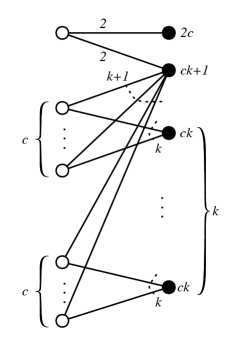
Figure 5: In this example, $R_{min}$ is equal to a constant $c$, i.e., every bid is at most $1/c$ of the budget of the bidder. In the strict model, all keywords except the first must be allocated to the second bidder at a price of $k$ (or the remaining budget if it’s smaller). Thus, the total profit on this input for the strict model is at most $ck+3$. On the other hand, in our model, if we allocate the first keyword to the second bidder, and then the next $c-1$ keywords to the second bidder, that bidder’s budget is reduced to $k-1$. Thus, all of the remaining keywords can be allocated to the lower bidder at a price of $k-1$, for a total revenue exceeding $ck(k-1)$. For $k$ large, this ratio is $\Omega(k)=\Omega(m)$.

On the other hand, we show below that the optimal values of the two models of Goel et al. cannot be better than the optimal value of our model by more than a constant factor.

Theorem 15.

For any instance $A$, $OPT_{non-strict}\leq(2+1/R_{min})OPT_{strict}\leq 8(2+1/R_{min})OPT_{2P}$.

The first inequality is proved by Goel et al. [GMNS08], so we must only prove that $OPT_{strict}\leq 8OPT_{2P}$.

The core of our argument is a reduction from 2PAA to the First-Price Ad Auctions problem (1PAA), in which only one bidder is chosen for each keyword and that bidder pays the minimum of its bid and its remaining budget. Given an instance $A$ of 2PAA, we construct an instance $A^{\prime}$ of 1PAA problem by replacing each bid $b_{u,v}$ by

$$b^{\prime}_{u,v}\triangleq\max_{v^{\prime}\neq v~{}:~{}b_{u,v^{\prime}}\leq b_{u,v}}b_{u,v^{\prime}}\enspace.$$

Denote by $OPT_{1P}(A^{\prime})$ the optimal value of the first-price model on $A^{\prime}$. The following two lemmas prove Theorem 15 by relating both $OPT_{non-strict}(A)$ and $OPT_{2P}(A)$ to $OPT_{1P}(A^{\prime})$.

Lemma 16.

$OPT_{non-strict}(A)\leq OPT_{1P}(A^{\prime})$.

Proof.

For an instance $A$, we can view a non-strict second-price allocation of $A$ as a pair of (partial) functions $f_{1}$ and $f_{2}$ from the keywords $U$ to the bidders $V$, where $f_{1}$ maps each keyword to the bidder to which it is allocated and $f_{2}$ maps each keyword to the bidder acting as its second-price bidder. Thus, if $f_{1}(u)=v$ and $f_{2}(u)=v^{\prime}$ then $u$ is allocated to $v$ and the price $v$ pays is $b_{u,v^{\prime}}$. We have, for all such $u$, $v$, and $v^{\prime}$, that $b_{u,v^{\prime}}\leq b^{\prime}_{u,v}$.

We construct the first-price allocation on $A^{\prime}$ defined by $f_{1}$ and claim that the value of this first-price allocation is at least the value of the non-strict allocation defined by $f_{1}$ and $f_{2}$. It suffices to show that for any bidder $v$, the profit that the non-strict allocation gets from $v$ is at most the profit that the first-price allocation gets from $v$, or in other words,

$$\min\left(B_{v},\sum_{u:f_{1}(u)=v}b_{u,f_{2}(u)}\right)\leq\min\left(B_{v},\sum_{u:f_{1}(u)=v}b^{\prime}_{u,v}\right)\enspace.$$

This inequality follows trivially from the fact that $b_{u,f_{2}(u)}\leq b^{\prime}_{u,f_{1}(u)}$ for all allocated keywords $u$, and hence the lemma follows. ∎

Lemma 17.

$OPT_{1P}(A^{\prime})\leq 8OPT_{2P}(A)$.

Proof.

Given an optimal first-price allocation of $A^{\prime}$, we can assume without loss of generality that each bidder’s budget can only be exhausted by the last keyword allocated to it, or, more formally, if $u_{1},u_{2},\ldots u_{k}$ are the keywords that are allocated to a bidder $v$ and they come in that order, then we can assume that $\sum_{i=1}^{k-1}b^{\prime}_{u_{i},v}<B_{v}$. The reason for this is that if for some $j<k$, $\sum_{i=1}^{j-1}b^{\prime}_{u_{i},v}<B_{v}$ and $\sum_{i=1}^{j}b^{\prime}_{u_{i},v}\geq B_{v}$, then we can ignore the allocation of $u_{j+1},\ldots u_{k}$ to $v$ without losing any profit.

With this assumption, we design a randomized algorithm that constructs a second-price allocation on $A$ whose expected value in our model is at least $1/8$ of the first-price allocation’s value. Viewing the first-price allocation of $A^{\prime}$ as a (partial) function $f$ from the keywords $U$ to the bidders $V$ and denoting by $s(u,v)$ the bidder $v^{\prime}$ for which $b_{v^{\prime}u}=b^{\prime}_{vu}$, the algorithm is as follows.

Random Construction: Randomly mark each bidder with probability $1/2$. For each unmarked bidder $v$:         Let $S_{v}=\emptyset$.         For each keyword $u$ such that $f(u)=v$:              If $s(u,v)$ is marked: $S_{v}=S_{v}\cup\{u\}$.         Assume that $S_{v}=\{u_{1},u_{2},\ldots u_{k}\}$, where $u_{1},u_{2},\ldots u_{k}$ come in that order.              If $\sum_{i=1}^{k}b^{\prime}_{u_{i},v}\leq B_{v}$:                   Let $f_{1}(u_{i})=v$ and $f_{2}(u_{i})=s(u_{i},v)$ for all $i\leq k$.              Else:                   If $\sum_{i=1}^{k-1}b^{\prime}_{u_{i},v}\geq b^{\prime}_{u_{k},v}$: let $f_{1}(u_{i})=v$ and $f_{2}(u_{i})=s(u_{i},v)$ for all $i\leq k-1$.                   Else: let $f_{1}(u_{k})=v$ and $f_{2}(u_{k})=s(u_{k},v)$.

We claim that for the $f_{1}$ and $f_{2}$ defined by this construction, whenever $f(u_{i})$ is set to $v$, the profit from that allocation is $b^{\prime}_{u_{i},v}$. This is not trivial because in our model, if a bidder’s remaining budget is smaller than its bid for a keyword, it changes its bid for that keyword to its remaining budget. However, one can easily verify that in all cases, if we set $f_{1}(u_{i})=v$ and $f_{2}(u_{i})=s(u_{i},v)$, the remaining budget of $v$ is at least $b^{\prime}_{u_{i},v}=b_{u_{i},s(u_{i},v)}$. Thus, the (modified) bid of $f_{1}(u_{i})$ for $u_{i}$ is still at least the original bid of $f_{2}(u_{i})$ for $u_{i}$.

We claim that the expected value of the second-price allocation defined by $f_{1}$ and $f_{2}$ is at least $1/8OPT_{1P}(A^{\prime})$. For each bidder $v$, let $X_{v}$ be the random variable denoting the profit that $f_{1}$ and $f_{2}$ get from $v$, and let $Y_{v}$ be the profit that $f$ gets from $v$. We have $OPT_{1P}(A^{\prime})=\sum_{v}Y_{v}$, so it suffices to show that $E(X_{v})\geq 1/8Y_{v}$ for all $v\in V$.

Consider any $v\in V$ that is unmarked. Let $T_{v}=\{u:f(u)=v\}$. If $\sum_{u\in S_{v}}b^{\prime}_{u,v}\leq B_{v}$ then $X_{v}=\sum_{u\in S_{v}}b^{\prime}_{u,v}$. If $\sum_{u\in S_{v}}b^{\prime}_{u,v}>B_{v}$ then $X_{v}\geq\sum_{u\in S_{v}}b^{\prime}_{u,v}/2$. Thus, in both case, we have

$$E[X_{v}|v\ \textrm{is unmarked}]\geq E[\sum_{u\in S_{v}}b^{\prime}_{u,v}/2|v\ \textrm{is unmarked}]=\sum_{u\in T_{v}}b^{\prime}_{u,v}/4=Y_{v}/4\enspace,$$

which implies

$$E[X_{v}]\geq E[X_{v}|v\ \textrm{is unmarked}]Pr[v\ \textrm{is unmarked}]=1/2\cdot Y_{v}/4=Y_{v}/8\enspace.$$

∎

Appendix B Proof of Theorem 12

In this appendix, we provide a full proof of Theorem 12. The proof presented here is quite similar to the simplified proof of Theorem 10 presented by Birnbaum and Mathieu [BM08]. For intuition into the proof presented here, the interested reader is referred to that work.

Let $G=(U_{G}\cup V,E_{G})$ be a bipartite graph and let $H=(U_{H}\cup V,E_{H})$ be a left $k$-copy of $G$. Let $\zeta:U_{H}\rightarrow U_{G}$ be a map that satisfies the conditions of Definition 11. Let $M_{G}\subseteq E_{G}$ be a maximum matching of $G$.

Let $\operatorname{Ranking}(H,\pi,\sigma)$ denote the matching constructed on $H$ for arrival order $\pi$, when the ranking is $\sigma$. Consider another process in which the vertices in $V$ arrive in the order given by $\sigma$ and are matched to the available vertex $u\in U_{H}$ that minimizes $\pi(u)$. Call the matching constructed by this process $\operatorname{Ranking}^{\prime}(H,\pi,\sigma)$. It is not hard to see that these matchings are identical, a fact that is proved in [KVV90].

Lemma 18 (Karp, Vazirani, and Vazirani [KVV90]).

For any permutations $\pi$ and $\sigma$, $\operatorname{Ranking}(H,\pi,\sigma)=\operatorname{Ranking}^{\prime}(H,\pi,\sigma)$.

The following monotonicity lemma shows that removing vertices in $H$ can only decrease the size of the matching returned by Ranking.

Lemma 19.

Let $\pi_{H}$ be an arrival order for the vertices in $U_{H}$, and let $\sigma_{H}$ be a ranking on the vertices in $V$. Suppose that $x$ is a vertex in $U_{H}\cup V$, and let $H^{\prime}=(U_{H^{\prime}},V_{H^{\prime}},E_{H^{\prime}})=H\setminus\left\{{x}\right\}$. Let $\pi_{H^{\prime}}$ and $\sigma_{H^{\prime}}$ be the orderings of $U_{H^{\prime}}$ and $V_{H^{\prime}}$ induced by $\pi_{H}$ and $\sigma_{H}$, respectively. Then $|\operatorname{Ranking}(H^{\prime},\pi_{H^{\prime}},\sigma_{H^{\prime}})|\leq|\operatorname{Ranking}(H,\pi_{H},\sigma_{H})|$.

Proof.

Suppose first that $x\in U_{H}$. In this case, $V=V_{H^{\prime}}$ and $\sigma_{H}=\sigma_{H^{\prime}}$. Let $Q_{t}(H)\subseteq V$ be the set of vertices matched to vertices in $U_{H}$ that arrive at or before time $t$ (under arrival order $\pi_{H}$ and ranking $\sigma_{H}$), and let $Q_{t}(H^{\prime})\subseteq V$ be the set of vertices matched to vertices in $U_{H^{\prime}}$ that arrive at or before time $t$ (under arrival order $\pi_{H^{\prime}}$ and ranking $\sigma_{H}$). We prove by induction on $t$ that $Q_{t-1}(H^{\prime})\subseteq Q_{t}(H)$, which by substituting $t=n$ is sufficient to prove the claim. The statement holds when $t=1$, since $Q_{0}(H^{\prime})=\emptyset$. Now supposing we have $Q_{t-2}(H^{\prime})\subseteq Q_{t-1}(H)$, we prove $Q_{t-1}(H^{\prime})\subseteq Q_{t}(H)$. Suppose that $t$ is at or before the time that $x$ arrives in $\pi_{H}$. Then clearly $Q_{t-1}(H^{\prime})=Q_{t-1}(H)\subseteq Q_{t}(H)$. Now suppose that $t$ is after the time that $x$ arrives in $\pi_{H}$. Let $u$ be the vertex that arrives at time $t-1$ in $\pi_{H^{\prime}}$. If $u$ is not matched by $\operatorname{Ranking}(H^{\prime},\pi_{H^{\prime}},\sigma_{H})$, then $Q_{t-1}(H^{\prime})=Q_{t-2}(H^{\prime})\subseteq Q_{t-1}(H)\subseteq Q_{t}(H)$. Now suppose that $u$ is matched by $\operatorname{Ranking}(H^{\prime},\pi_{H^{\prime}},\sigma_{H})$, say to vertex $v^{\prime}$. We show that $v^{\prime}\in Q_{t}(H)$, which by the induction hypothesis, is enough to prove that $Q_{t-1}(H^{\prime})\subseteq Q_{t}(H)$. Note that $u$ arrives at time $t$ in $\pi_{H}$. Let $v$ be the vertex to which $u$ is matched by $\operatorname{Ranking}(H,\pi_{H},\sigma_{H})$. If $v=v^{\prime}$, we are done, so suppose that $v\not=v^{\prime}$. Since $v\not\in Q_{t-1}(H)$, it follows by the induction hypothesis that $v\not\in Q_{t-2}(H^{\prime})$. Therefore, vertex $v$ is available to be matched to $u$ when it arrives in $\pi_{H^{\prime}}$. Since $\operatorname{Ranking}(H^{\prime},\pi_{H^{\prime}},\sigma_{H})$ matched $u$ to $v^{\prime}$ instead, $v^{\prime}$ must have a lower rank than $v$ in $\sigma_{H}$. Since $\operatorname{Ranking}(H,\pi_{H},\sigma_{H})$ chose $v$, vertex $v^{\prime}$ must have already been matched when vertex $u$ arrived at time $t$ in $\pi_{H}$, or, in other words, $v^{\prime}\in Q_{t-1}(H)\subseteq Q_{t}(H)$.

Now suppose that $x\in V$. In this case, $U_{H}=U_{H^{\prime}}$ and $\pi_{H}=\pi_{H^{\prime}}$. Let $R_{t}(H)\subseteq U_{H}$ be the set of vertices matched to vertices in $V$ that are ranked less than or equal to $t$ (under arrival order $\pi_{H}$ and ranking $\sigma_{H}$), and let $R_{t}(H^{\prime})\subseteq U_{H}$ be the set of vertices matched to vertices in $V$ that are ranked less than or equal to $t$ (under arrival order $\pi_{H}$ and ranking $\sigma_{H^{\prime}}$). Then by Lemma 18, we can apply the same argument as before to show that $R_{t-1}(H^{\prime})\subseteq R_{t}(H)$ for all $t$, which by substituting $t=n$, is sufficient to prove the claim. ∎

We define the following notation. For all $u_{G}\in U_{G}$, let $\zeta^{-1}(u_{G})$ be the set of all $u_{H}\in U_{H}$ such that $\zeta(u_{H})=u_{G}$, and for any subset $U_{G}^{\prime}\subseteq U_{G}$, let $\zeta^{-1}(U_{G}^{\prime})$ be the set of all $u_{H}\in U_{H}$ such that $\zeta(u_{H})\in U_{G}^{\prime}$. The following lemma shows that we can assume without loss of generality that $M_{G}$ is a perfect matching.

Lemma 20.

Let $U^{\prime}\subseteq U_{G}$ and $V^{\prime}\subseteq V$ be the subset of vertices that are in $M_{G}$. Let $G^{\prime}$ be the subgraph of $G$ induced by $U^{\prime}\cup V^{\prime}$, and let $H^{\prime}$ be the subgraph of $H$ induced by $\zeta^{-1}(U^{\prime})\cup V^{\prime}$. Then the expected size of the matching produced by Ranking on $H^{\prime}$ is no greater than the expected size of the matching produced by Ranking on $H$.

Proof.

The proof follows by repeated application of Lemma 19 for all $x$ that are not in $\zeta^{-1}(U^{\prime})\cup V^{\prime}$. ∎

In light of Lemma 20, to prove Theorem 12, it is sufficient to show that the expected size of the matching produced by Ranking on $H^{\prime}$ is at least $(1-1/e^{1/k}-o(1))|M_{G}|$. To simplify notation, we instead assume without loss of generality that $G=G^{\prime}$, and hence $G$ has a perfect matching. Let $n=OPT_{1P}=|M_{G}|=|V|$. Henceforth, fix an arrival order $\pi$. To simplify notation, we write $\operatorname{Ranking}(\sigma)$ to mean $\operatorname{Ranking}(H,\pi,\sigma)$.

Let $f:U_{H}\rightarrow V$ be a map such that for all $v\in V$, there are exactly $k$ vertices $u\in U_{H}$ such that $f(u)=v$. The existence of such a map $f$ follows from the assumption that $G$ has a perfect matching. For any vertex $v\in V$ let $f^{-1}(v)$ be the set of $u\in U_{H}$ such that $f(u)=v$. We proceed with the following two lemmas.

Lemma 21.

Let $u\in U_{H}$, and let $v=f(u)$. For any ranking $\sigma$, if $v$ is not matched by $\operatorname{Ranking}(\sigma)$, then $u$ is matched to a vertex whose rank is less than the rank of $v$ in $\sigma$.

Proof.

If $v$ is not matched by $\operatorname{Ranking}(\sigma)$, then since there is an edge between $u$ and $v$, it was available to be matched to $u$ when it arrived. Therefore, by the behavior of $\operatorname{Ranking}$, $u$ must have been matched to a vertex of lower rank. ∎

Lemma 22.

Let $u\in U_{H}$, and let $v=f(u)$. Fix an integer $t$ such that $1\leq t\leq n$. Let $\sigma$ be a permutation, and let $\sigma^{\prime}$ be the permutation obtained from $\sigma$ by removing vertex $v$ and putting it back in so its rank is $t$. If $v$ is not matched by $\operatorname{Ranking}(\sigma^{\prime})$, then $u$ must be matched by $\operatorname{Ranking}(\sigma)$ to a vertex whose rank in $\sigma$ is less than or equal to $t$.

Proof.

For the proof, it is convenient to invoke Lemma 18 and consider $\operatorname{Ranking}^{\prime}(\sigma)$ and $\operatorname{Ranking}^{\prime}(\sigma^{\prime})$ instead of $\operatorname{Ranking}(\sigma)$ and $\operatorname{Ranking}(\sigma^{\prime})$. In the process by which $\operatorname{Ranking}^{\prime}$ constructs its matching, call the moment that the $t^{\textrm{th}}$ vertex in $V$ arrives time $t$. For any $1\leq s\leq n$, let $R_{s}(\sigma)$ (resp., $R_{s}(\sigma^{\prime})$) be the set of vertices in $U_{H}$ matched by time $s$ in $\sigma$ (resp., $\sigma^{\prime}$). By Lemma 21, if $v$ is not matched by $\operatorname{Ranking}(\sigma^{\prime})$, then $u$ must be matched to a vertex $v^{\prime}$ in $\operatorname{Ranking}(\sigma^{\prime})$ such that $\sigma^{\prime}(v^{\prime})<\sigma^{\prime}(v)$. Hence $u\in R_{t-1}(\sigma^{\prime})$. We prove the lemma by showing that $R_{t-1}(\sigma^{\prime})\subseteq R_{t}(\sigma)$. Let $\tilde{t}$ be the time that $v$ arrives in $\sigma$. Then if $\tilde{t}\geq t$, the two orders $\sigma$ and $\sigma$ are identical through time $t$, which implies that $R_{t-1}(\sigma^{\prime})=R_{t-1}(\sigma)\subseteq R_{t}(\sigma)$.

Now, in the case that $\tilde{t}<t$, we prove that for $1\leq s\leq t$, $R_{s-1}(\sigma^{\prime})\subseteq R_{s}(\sigma)$. The proof, which is similar to the proof of Lemma 19, proceeds by induction on $s$. When $s=0$, the claim clearly holds, since $R_{0}(\sigma^{\prime})=\emptyset$. Now, supposing that $R_{s-2}(\sigma^{\prime})\subseteq R_{s-1}(\sigma)$, we prove that $R_{s-1}(\sigma^{\prime})\subseteq R_{s}(\sigma)$. If $s\leq\tilde{t}$, then the two orders $\sigma$ and $\sigma^{\prime}$ are identical through time $s$, so $R_{s-1}(\sigma^{\prime})=R_{s-1}(\sigma)\subseteq R_{s}(\sigma)$. Now suppose that $s>\tilde{t}$. Then the vertex that arrives at time $s-1$ in $\sigma^{\prime}$ is the same as the vertex that arrives at time $s$ in $\sigma$. Call this vertex $w$. If $w$ is not matched by $\operatorname{Ranking}^{\prime}(\sigma^{\prime})$, then $R_{s-1}(\sigma^{\prime})=R_{s-2}(\sigma^{\prime})$, and we are done by the induction hypothesis. Now suppose that $w$ is matched to vertex $x^{\prime}$ by $\operatorname{Ranking}^{\prime}(\sigma^{\prime})$ and to vertex $x$ by $\operatorname{Ranking}^{\prime}(\sigma)$. If $x=x^{\prime}$, then again we are done by the induction hypothesis, so suppose that $x\neq x^{\prime}$. Since $x$ was available at time $s-1$ in $\sigma$, we have $x\not\in R_{s-1}(\sigma)$, and by the induction hypothesis $x\not\in R_{s-2}(\sigma^{\prime})$. Hence, $x$ was available at time $s-1$ in $\sigma^{\prime}$. Since $\operatorname{Ranking}^{\prime}(\sigma^{\prime})$ matched $w$ to $x^{\prime}$, it must be that $\pi(x^{\prime})<\pi(x)$. This implies that $x^{\prime}$ must be matched when $w$ arrives at time $s$ in $\sigma$, or in other words, $x^{\prime}\in R_{s-1}(\sigma)\subseteq R_{s}(\sigma)$. By the induction hypothesis, we are done. ∎

Lemma 23.

For $1\leq t\leq n$, let $x_{t}$ denote the probability over $\sigma$ that the vertex ranked $t$ in $V$ is matched by $\operatorname{Ranking}(\sigma)$. Then

$$1-x_{t}\leq\frac{1}{kn}\sum_{s=1}^{t}x_{s}\enspace.$$ (9)

Proof.

Let $\sigma$ be permutation chosen uniformly at random, and let $\sigma^{\prime}$ be a permutation obtained from $\sigma$ by choosing a vertex $v\in V$ uniformly at random, taking it out of $\sigma$, and putting it back so that its rank is $t$. Note that both $\sigma$ and $\sigma^{\prime}$ are distributed uniformly at random among all permutations. Let $u$ be a vertex chosen uniformly at random from $f^{-1}(v)$. Note that conditioned on $\sigma$, $u$ is equally likely to be any of the $kn$ vertices in $U_{H}$. Let $R_{t}$ be the set of vertices in $U_{H}$ that are matched by $\operatorname{Ranking}(\sigma)$ to a vertex of rank $t$ or lower in $\sigma$. Lemma 22 states that if $v$ is not matched by $\operatorname{Ranking}(\sigma^{\prime})$, then $u\in R_{t}$. The expected size of $R_{t}$ is $\sum_{1\leq s\leq t}x_{s}$. Hence, the probability that $u\in R_{t}$, conditioned on $\sigma$, is $(1/(kn))\sum_{1\leq s\leq t}x_{s}$. The lemma follows because the probability that $v$ is not matched by $\operatorname{Ranking}(\sigma^{\prime})$ is $1-x_{t}$. ∎

We are now ready to prove Theorem 12.

Proof of Theorem 12.

For $0\leq t\leq n$, let $S_{t}=\sum_{1\leq s\leq t}x_{s}$. Then the expected size of the matching returned by Ranking on $H$ is $S_{n}$. Rearranging (9) yields, for $1\leq t\leq n$,

$$S_{t}\geq\left({\frac{kn}{kn+1}}\right)\left({1+S_{t-1}}\right),$$

which by induction implies that $S_{t}\geq\sum_{1\leq s\leq t}(kn/(kn+1))^{s}$, and hence

$$S_{n}\geq\sum_{s=1}^{n}\left({\frac{kn}{kn+1}}\right)^{s}=kn\left({1-\left({1-\frac{1}{kn+1}}\right)^{n}}\right)=kn\left({1-\frac{1}{e^{1/k}}+o(1)}\right)\enspace.$$

∎

References

- [ABK+08] Yossi Azar, Benjamin Birnbaum, Anna R. Karlin, Claire Mathieu, and C. Thach Nguyen. Improved approximation algorithms for budgeted allocations. In ICALP ’08 (LNCS 5125), pages 186–197. Springer, 2008.
- [AM04] Nir Andelman and Yishay Mansour. Auctions with budget constraints. In SWAT ’04 (LNCS 3111), pages 26–38. Springer, 2004.
- [AMT07] Zoe Abrams, Ofer Mendelevitch, and John Tomlin. Optimal delivery of sponsored search advertisements subject to budget constraints. In EC ’07, 2007.
- [BJN07] Niv Buchbinder, Kamal Jain, and Joseph (Seffi) Naor. Online primal-dual algorithms for maximizing ad-auctions revenue. In ESA ’07 (LNCS 4698), pages 253–264. Springer, 2007.
- [BM08] Benjamin Birnbaum and Claire Mathieu. On-line bipartite matching made simple. SIGACT News, 39(1):80–87, 2008.
- [CC06] Miroslav Chlebík and Janka Chlebíková. Complexity of approximating bounded variants of optimization problems. Theoretical Computer Science, 354(3):320–338, 2006.
- [CG08] Deeparnab Chakrabarty and Gagan Goel. On the approximability of budgeted allocations and improved lower bounds for submodular welfare maximization and gap. In FOCS ’08, pages 687–696, 2008.
- [CK00] Chandra Chekuri and Sanjeev Khanna. A PTAS for the multiple knapsack problem. In SODA ’00, pages 213–222, 2000.
- [DH09] Nikhil R. Devanur and Thomas P. Hayes. The adwords problem: Online keyword matching with budgeted bidders under random permutations. In EC ’09, 2009.
- [DS06] Shahar Dobzinski and Michael Schapira. An improved approximation algorithm for combinatorial auctions with submodular bidders. In SODA ’06, pages 1064–1073, 2006.
- [EOS07] Benjamin Edelman, Michael Ostrovsky, and Michael Schwarz. Internet advertising and generalized second-price auction: Selling billions of dollars worth of keywords. American Economic Review, 97:242–259, 2007.
- [FGMS06] Lisa Fleischer, Michel X. Goemans, Vahab S. Mirrokni, and Maxim Sviridenko. Tight approximation algorithms for maximum general assignment problems. In SODA ’06, pages 611–620, 2006.
- [FV06] Uriel Feige and Jan Vondrak. Approximation algorithms for allocation problems: Improving the factor of 1 - 1/e. FOCS ’06, pages 667–676, 2006.
- [GJ79] Michael R. Garey and David S. Johnson. Computers and Intractability. W. H. Freeman and Company, 1979.
- [GM08] Gagan Goel and Aranyak Mehta. Online budgeted matching in random input models with applications to adwords. In SODA ’08, pages 982–991, 2008.
- [GMNS08] Ashish Goel, Mohammad Mahdian, Hamid Nazerzadeh, and Amin Saberi. Advertisement allocation for generalized second pricing schemes. In Workshop on Sponsored Search Auctions, 2008.
- [KLMM05] Subhash Khot, Richard J. Lipton, Evangelos Markakis, and Aranyak Mehta. Inapproximability results for combinatorial auctions with submodular utility functions. In WINE ’05 (LNCS 3828, pages 92–101. Springer, 2005.
- [KVV90] R. M. Karp, U. V. Vazirani, and V. V. Vazirani. An optimal algorithm for on-line bipartite matching. In STOC ’90, pages 352–358, 1990.
- [LLN06] Benny Lehmann, Daniel Lehmann, and Noam Nisan. Combinatorial auctions with decreasing marginal utilities. Games and Economic Behavior, 55(2):270–296, 2006.
- [LPSV07] Sebastien Lahaie, David M. Pennock, Amin Saberi, and Rakesh V. Vohra. Sponsored search auctions. In Noam Nisan, Tim Roughgarden, Eva Tardos, and Vijay V. Vazirani, editors, Algorithmic Game Theory, pages 699–716. Cambridge University Press, 2007.
- [MNS07] Mohammad Mahdian, Hamid Nazerzadeh, and Amin Saberi. Allocating online advertisement space with unreliable estimates. In EC ’07, pages 288–294, 2007.
- [MSV08] Vahab Mirrokni, Michael Schapira, and Jan Vondrak. Tight information-theoretic lower bounds for welfare maximization in combinatorial auctions. In EC ’08, 2008.
- [MSVV07] Aranyak Mehta, Amin Saberi, Umesh Vazirani, and Vijay Vazirani. Adwords and generalized online matching. J. ACM, 54(5):22, 2007.
- [Sri08] Aravind Srinivasan. Budgeted allocations in the full-information setting. In APPROX ’08 (LNCS 5171), pages 247–253. Springer, 2008.
- [ST93] David Shmoys and Eva Tardos. An approximation algorithm for the generalized assignment problem. Mathematical Programming, 62:461–474, 1993.
- [Var07] Hal R. Varian. Position auctions. International Journal of Industrial Organization, 25:1163–1178, 2007.
- [Von08] Jan Vondrak. Optimal approximation for the submodular welfare problem in the value oracle model. In STOC ’08, pages 67–74, 2008.
- [Yao77] Andrew Yao. Probabilistic computations: Toward a unified measure of complexity. In FOCS ’77, pages 222–227, 1977.