A Rate-Distortion Perspective on Multiple Decoding Attempts for Reed-Solomon Codes

Phong S. Nguyen, Henry D. Pfister, and Krishna R. Narayanan
Department of Electrical and Computer Engineering, Texas A&M University
College Station, TX 77840, U.S.A.
{psn, hpfister, krn}@tamu.edu
Abstract

Recently, a number of authors have proposed decoding schemes for Reed-Solomon (RS) codes based on multiple trials of a simple RS decoding algorithm. In this paper, we present a rate-distortion (R-D) approach to analyze these multiple-decoding algorithms for RS codes. This approach is first used to understand the asymptotic performance-versus-complexity trade-off of multiple error-and-erasure decoding of RS codes. By defining an appropriate distortion measure between an error pattern and an erasure pattern, the condition for a single error-and-erasure decoding to succeed reduces to a form where the distortion is compared to a fixed threshold. Finding the best set of erasure patterns for multiple decoding trials then turns out to be a covering problem which can be solved asymptotically by rate-distortion theory. Next, this approach is extended to analyze multiple algebraic soft-decision (ASD) decoding of RS codes. Both analytical and numerical computations of the R-D functions for the corresponding distortion measures are discussed. Simulation results show that proposed algorithms using this approach perform better than other algorithms with the same complexity.

I Introduction

Reed-Solomon (RS) codes are one of the most widely used error-correcting codes in digital communication and data storage systems. This is primarily due to the fact that RS codes are maximum distance separable (MDS) codes, can correct long bursts of errors, and have efficient hard-decision decoding (HDD) algorithms, such as the Berlekamp-Massey (BM) algorithm, which can correct up to half the minimum distance ($d_{min})$ of the code. Anย (n,k)๐‘›๐‘˜(n,k)ย RS code of lengthย n๐‘›nย and dimensionย k๐‘˜k is known to haveย dmโ€‹iโ€‹n=nโˆ’k+1subscript๐‘‘๐‘š๐‘–๐‘›๐‘›๐‘˜1d_{min}=n-k+1ย due to its MDS nature.

Since the arrival of RS codes, people have put a considerable effort into improving the decoding performance at the expense of complexity. A breakthrough result of Guruswami and Sudan (GS) introduces a hard-decision list-decoding algorithm based on algebraic bivariate interpolation and factorization techniques that can correct errors beyond half the minimum distance of the code [1]. Nevertheless, HDD algorithms do not fully exploit the information provided by the channel output. Koetter and Vardy (KV) later extended the GS decoder to an algebraic soft-decision (ASD) decoding algorithm by converting the probabilities observed at the channel output into algebraic interpolation conditions in terms of a multiplicity matrix [2]. Both of these algorithms however have significant computational complexity. Thus, multiple runs of error-and-erasure and error-only decoding with some low complexity algorithm, such as the BM algorithm, has renewed the interest of researchers. These algorithms essentially first construct a set of either erasure patterns [3, 4], test patterns [5], or patterns combining both [6] and then attempt to decode using each pattern. There has also been recent interest in lowering the complexity per decoding trial as can be seen in [7, 8, 9].

In the scope of multiple error-and-erasure decoding, there have been several algorithms using different sets of erasure patterns. After multiple decoding trials, these algorithms produce a list of candidate codewords and then pick the best codeword on this list, whose size is usually small. The nature of multiple error-and-erasure decoding is to erase some of the least reliable symbols since those symbols are more prone to be erroneous. The first algorithm of this type is called Generalized Minimum Distance (GMD) [3] and it repeats error-and-erasure decoding while successively erasing an even number of the least reliable positions (LRPs) (assuming thatย dmโ€‹iโ€‹nsubscript๐‘‘๐‘š๐‘–๐‘›d_{min}ย is odd). More recent work by Lee and Kumar [4] proposes a soft-information successive (multiple) error-and-erasure decoding (SED) that achieves better performance but also increases the number of decoding attempts. Literally, the Lee-Kumarโ€™s SED$(l,f)$ย algorithm runs multiple error-and-erasure decoding trials with every combination of an even numberย โ‰คfabsent๐‘“\leq fย of erasures within theย l๐‘™lย LRPs.

A natural question that arises is how to construct the โ€œbestโ€ set of erasure patterns for multiple error-and-erasure decoding. Inspired by this, we first design a rate-distortion framework to analyze the asymptotic trade-off between performance and complexity of multiple error-and-erasure decoding of RS codes. The framework is also extended to analyze multiple algebraic soft-decision decoding (ASD). Next, we proposed a group of multiple-decoding algorithms based on this approach that achieve better performance-versus-complexity trade-off than other algorithms. The multiple-decoding algorithm that achieves the best trade-off turns out to be a multiple error-only decoding using the set of patterns generated by random codes combining with covering codes. These are the main results of this paper.

I-A Outline of the paper

The paper is organized as follows. In Section II, we design an appropriate distortion measure and present a rate-distortion framework to analyze the performance-versus-complexity trade-off of multiple error-and-erasure decoding of RS codes. Also in this section, we propose a general multiple-decoding algorithm that can be applied to error-and-erasure decoding. Then, in Section III, we discuss a numerical computation of R-D function which is needed for the proposed algorithm. In Section IV, we analyze both bit-level and symbol-level ASD decoding and design distortion measures so that they can fit into the general algorithm. In Section V, we offer some extensions that help the algorithm achieve better performance and running time. Simulation results are presented in Section VI and finally, conclusion is provided in Section VII.

II Multiple Error-and-Erasure Decoding

In this section, we set up a rate-distortion framework to analyze multiple attempts of conventional hard decision error-and-erasure decoding.

Letย ๐”ฝ2qsubscript๐”ฝsuperscript2๐‘ž\mathbb{F}_{2^{q}}ย be the Galois field withย 2qsuperscript2๐‘ž2^{q}ย elements denoted asย ฮฑ1,ฮฑ2,โ€ฆ,ฮฑ2qsubscript๐›ผ1subscript๐›ผ2โ€ฆsubscript๐›ผsuperscript2๐‘ž\alpha_{1},\alpha_{2},\ldots,\alpha_{2^{q}}. We consider an $(n,k)$ย RS code of lengthย n๐‘›n, dimensionย k๐‘˜k overย ๐”ฝ2qsubscript๐”ฝsuperscript2๐‘ž\mathbb{F}_{2^{q}}. Assume that we transmit a codewordย ๐œ=(c1,c2,โ€ฆ,cn)โˆˆ๐”ฝ2qn๐œsubscript๐‘1subscript๐‘2โ€ฆsubscript๐‘๐‘›superscriptsubscript๐”ฝsuperscript2๐‘ž๐‘›\mathbf{c}=(c_{1},c_{2},\ldots,c_{n})\in\mathbb{F}_{2^{q}}^{n}ย over some channel and receive a vectorย ๐ซ=(r1,r2,โ€ฆ,rn)โˆˆ๐’ดn๐ซsubscript๐‘Ÿ1subscript๐‘Ÿ2โ€ฆsubscript๐‘Ÿ๐‘›superscript๐’ด๐‘›\mathbf{r}=(r_{1},r_{2},\ldots,r_{n})\in\mathcal{Y}^{n}ย whereย ๐’ด๐’ด\mathcal{Y}ย is the receive alphabet for a single RS symbol. In this paper, we assume that $\mathcal{Y}=\mathbb{R}^{q}$ and all simulations are based on transmitting each of the $q$ bits in a symbol using Binary Phase-Shift Keying (BPSK) on an Additive White Gaussian Noise (AWGN) channel. For each codeword indexย i๐‘–i, letย ฯ€i:{1,2,โ€ฆ,2q}โ†’{1,2,โ€ฆ,2q}:subscript๐œ‹๐‘–โ†’12โ€ฆsuperscript2๐‘ž12โ€ฆsuperscript2๐‘ž\pi_{i}:\{1,2,\ldots,2^{q}\}\rightarrow\{1,2,\ldots,2^{q}\}ย be the permutation given by sortingย pi,j=Prโก(ci=ฮฑj|๐ซ)subscript๐‘๐‘–๐‘—Prsubscript๐‘๐‘–conditionalsubscript๐›ผ๐‘—๐ซp_{i,j}=\Pr(c_{i}=\alpha_{j}|\mathbf{r})ย in decreasing order so thatย pi,ฯ€iโ€‹(1)โ‰ฅpi,ฯ€iโ€‹(2)โ‰ฅโ€ฆโ‰ฅpi,ฯ€iโ€‹(2q)subscript๐‘๐‘–subscript๐œ‹๐‘–1subscript๐‘๐‘–subscript๐œ‹๐‘–2โ€ฆsubscript๐‘๐‘–subscript๐œ‹๐‘–superscript2๐‘žp_{i,\pi_{i}(1)}\geq p_{i,\pi_{i}(2)}\geq\ldots\geq p_{i,\pi_{i}(2^{q})}. Then, we can specifyย yi,j=ฮฑฯ€iโ€‹(j)subscript๐‘ฆ๐‘–๐‘—subscript๐›ผsubscript๐œ‹๐‘–๐‘—y_{i,j}=\alpha_{\pi_{i}(j)}ย as theย j๐‘—j-th most reliable symbol forย j=1,โ€ฆ,2q๐‘—1โ€ฆsuperscript2๐‘žj=1,\ldots,2^{q}ย at codeword indexย i๐‘–i. To obtain the reliability of the codeword positions (indices), we construct the permutationย ฯƒ:{1,2,โ€ฆ,n}โ†’{1,2,โ€ฆ,n}:๐œŽโ†’12โ€ฆ๐‘›12โ€ฆ๐‘›\sigma:\{1,2,\ldots,n\}\rightarrow\{1,2,\ldots,n\}ย given by sorting the probabilitiesย pi,ฯ€iโ€‹(1)subscript๐‘๐‘–subscript๐œ‹๐‘–1p_{i,\pi_{i}(1)}ย of the most likely symbols in increasing order. Thus, codeword positionย ฯƒโ€‹(i)๐œŽ๐‘–\sigma(i)ย is theย i๐‘–i-th LRP. These above notations will be used throughout this paper.

Example 1

Considerย n=3๐‘›3n=3ย andย q=2๐‘ž2q=2. Assume that we have the probabilityย pi,jsubscript๐‘๐‘–๐‘—p_{i,j} written in a matrix form as follows

$$\mathbf{P}=\left(\begin{array}[]{ccc}0.01&0.01&\mathbf{0.93}\\ \mathbf{0.94}&0.03&0.04\\ 0.03&\mathbf{0.49}&0.01\\ 0.02&0.47&0.02\end{array}\right)\,\,\mbox{\mbox{where}}\,\,p_{i,j}=[\mathbf{P}]_{j,i}$$

thenย ฯ€1โ€‹(1,2,3,4)=(2,3,4,1),ฯ€2โ€‹(1,2,3,4)=(3,4,2,1),ฯ€3โ€‹(1,2,3,4)=(1,2,4,3)formulae-sequencesubscript๐œ‹112342341formulae-sequencesubscript๐œ‹212343421subscript๐œ‹312341243\pi_{1}(1,2,3,4)=(2,3,4,1),\pi_{2}(1,2,3,4)=(3,4,2,1),\pi_{3}(1,2,3,4)=(1,2,4,3)ย andย ฯƒโ€‹(1,2,3)=(2,3,1)๐œŽ123231\sigma(1,2,3)=(2,3,1).

Condition 1

(Classical decoding threshold, see [10, 11]): Ifย e๐‘’eย symbols are erased, a conventional hard-decision error-and-erasure decoder such as the BM algorithm is able to correctย ฮฝ๐œˆ\nuย errors in unerased positions if

$$2\nu+e<n-k+1.$$ (1)

II-A Conventional error and erasure patterns.

Definition 1

(Conventional error and erasure patterns) We defineย xnโˆˆโ„ค2nโ‰œ{0,1}nsuperscript๐‘ฅ๐‘›superscriptsubscriptโ„ค2๐‘›โ‰œsuperscript01๐‘›x^{n}\in\mathbb{Z}_{2}^{n}\triangleq\{0,1\}^{n}ย andย x^nโˆˆโ„ค2nsuperscript^๐‘ฅ๐‘›superscriptsubscriptโ„ค2๐‘›\hat{x}^{n}\in\mathbb{Z}_{2}^{n}ย as an error pattern and an erasure pattern respectively, whereย xi=0subscript๐‘ฅ๐‘–0x_{i}=0ย means that an error occurs (i.e. the most likely symbol is incorrect) andย x^i=0subscript^๐‘ฅ๐‘–0\hat{x}_{i}=0ย means that an erasure occurs at indexย i๐‘–i.

Example 2

Ifย dmโ€‹iโ€‹nsubscript๐‘‘๐‘š๐‘–๐‘›d_{min}ย is odd then $\{111111\ldots,001111\ldots,000011\ldots,\ldots\}$ is the set of erasure patterns for the GMD algorithm. For the SED$(3,2)$ย algorithm, the set of erasure patterns has the formย {111111โ€‹โ€ฆ,001111โ€‹โ€ฆ,010111โ€‹โ€ฆ,100111โ€‹โ€ฆ}111111โ€ฆ001111โ€ฆ010111โ€ฆ100111โ€ฆ\{111111\ldots,001111\ldots,010111\ldots,100111\ldots\}. Here, in each erasure pattern the letters are written in increasing reliability order of the codeword positions.

Let us revisit the question how to construct the best set of erasure patterns for multiple error-and-erasure decoding. First, it can be seen that a multiple error-and-erasure decoding succeeds if the condition (1) is satisfied during at least one round of decoding. Thus, our approach is to design a distortion measure that converts the condition (1) into a form where the distortion between an error patternย xnsuperscript๐‘ฅ๐‘›x^{n}ย and an erasure patternย x^nsuperscript^๐‘ฅ๐‘›\hat{x}^{n}, denoted asย dโ€‹(xn,x^n)๐‘‘superscript๐‘ฅ๐‘›superscript^๐‘ฅ๐‘›d(x^{n},\hat{x}^{n}), is less than a fixed threshold.

Definition 2

Given a letter-by-letter distortion measureย ฮด๐›ฟ\delta, the distortion between an error patternย xnsuperscript๐‘ฅ๐‘›x^{n}ย and an erasure patternย x^nsuperscript^๐‘ฅ๐‘›\hat{x}^{n}ย is defined by

$$d(x^{n},\hat{x}^{n})=\sum_{i=1}^{n}\delta(x_{i},\hat{x}_{i}).$$
Proposition 1

If we choose the letter-by-letter distortion measureย ฮด:โ„ค2ร—โ„ค2โ†’โ„โ‰ฅ0:๐›ฟโ†’subscriptโ„ค2subscriptโ„ค2subscriptโ„absent0\delta:\mathbb{Z}_{2}\times\mathbb{Z}_{2}\rightarrow\mathbb{R}_{\geq 0}ย  as follows

$$\begin{array}[]{cc}\delta(0,0)=1&\delta(0,1)=2\\ \delta(1,0)=1&\delta(1,1)=0\end{array}$$ (2)

then the condition (1) for a successful error-and-erasure decoding then reduces to the form where the distortion is less than a fixed threshold

$$d(x^{n},\hat{x}^{n})<n-k+1.$$
Proof:

First, we define ฯ‡s,tโ‰œ|{iโˆˆ{1,2,โ€ฆ,n}:xi=s,x^i=t}|โ‰œsubscript๐œ’๐‘ ๐‘กconditional-set๐‘–12โ€ฆ๐‘›formulae-sequencesubscript๐‘ฅ๐‘–๐‘ subscript^๐‘ฅ๐‘–๐‘ก\chi_{s,t}\triangleq\left|\{i\in\left\{1,2,\ldots,n\right\}:x_{i}=s,\hat{x}_{i}=t\}\right| to count the number ofย (xi,x^i)subscript๐‘ฅ๐‘–subscript^๐‘ฅ๐‘–(x_{i},\hat{x}_{i})ย pairs equal toย (s,t)๐‘ ๐‘ก(s,t)ย for everyย s,tโˆˆ{0,1}๐‘ ๐‘ก01s,t\in\{0,1\}. Noticing thatย e=ฯ‡0,0+ฯ‡1,0๐‘’subscript๐œ’00subscript๐œ’10e=\chi_{0,0}+\chi_{1,0}ย andย ฮฝ=ฯ‡0,1๐œˆsubscript๐œ’01\nu=\chi_{0,1}, the condition (1) for one error-and-erasure decoding attempt to succeed becomes ย 2โ€‹ฯ‡0,1+ฯ‡0,0+ฯ‡1,0<nโˆ’k+12subscript๐œ’01subscript๐œ’00subscript๐œ’10๐‘›๐‘˜12\chi_{0,1}+\chi_{0,0}+\chi_{1,0}<n-k+1. By seeing thatย dโ€‹(xn,x^n)=2โ€‹ฯ‡0,1+ฯ‡0,0+ฯ‡1,0๐‘‘superscript๐‘ฅ๐‘›superscript^๐‘ฅ๐‘›2subscript๐œ’01subscript๐œ’00subscript๐œ’10d(x^{n},\hat{x}^{n})=2\chi_{0,1}+\chi_{0,0}+\chi_{1,0}ย we conclude the proof. โˆŽ

Next, we try to maximize the chance that this successful decoding condition is satisfied by at least one of the decoding attempts (i.e.ย dโ€‹(xn,x^n)<nโˆ’k+1๐‘‘superscript๐‘ฅ๐‘›superscript^๐‘ฅ๐‘›๐‘›๐‘˜1d(x^{n},\hat{x}^{n})<n-k+1ย for at least one erasure patternsย x^nsuperscript^๐‘ฅ๐‘›\hat{x}^{n}). Mathematically, we want to build a setย โ„ฌโ„ฌ\mathcal{B}ย of no more thanย 2Rsuperscript2๐‘…2^{R}ย erasure patternsย x^nsuperscript^๐‘ฅ๐‘›\hat{x}^{n}ย in order to

$$\max_{\mathcal{B}:|\mathcal{B}|\leq 2^{R}}\Pr\{\min_{\hat{x}^{n}\in\mathcal{B}}d(x^{n},\hat{x}^{n})<n-k+1\}.$$ (3)

The exact answer to this problem is difficult to find. However, one can see it as a covering problem where one wants to cover the space of error patterns using a minimum number of balls centered at the chosen erasure patterns.

This view leads to an asymptotic solution of the problem based on rate-distortion theory. More precisely, we view the error patternย xnsuperscript๐‘ฅ๐‘›x^{n}ย as a source sequence and the erasure patternย x^nsuperscript^๐‘ฅ๐‘›\hat{x}^{n}ย as a reproduction sequence.

Error pattern Erasure pattern

Rate-distortion theory shows that the setย โ„ฌโ„ฌ\mathcal{B}ย ofย 2Rsuperscript2๐‘…2^{R}ย reproduction sequences can be generated randomly so that

$$\lim_{n\rightarrow\infty}E_{\hat{x}^{n}\in\mathcal{B}}\left[d(x^{n},\hat{x}^{n})\right]\leq D$$

where the distortionย D๐ทDย is minimized for a given rateย R๐‘…R. Thus, for large enoughย n๐‘›n, we have

$$\min_{\hat{x}^{n}\in\mathcal{B}}d(x^{n},\hat{x}^{n})\leq D$$

with high probability. Here,ย R๐‘…Rย andย D๐ทDย are closely related to the complexity and the performance, respectively, of the decoding algorithm. Therefore, we characterize the trade-off between those two aspects using the relationship betweenย R๐‘…Rย andย D๐ทD.

II-B Generalized error and erasure patterns

In this subsection, we consider a generalization of the conventional error and erasure patterns under the same framework to make better use of the soft information. At each index of the RS codeword, beside erasing the symbol we can try to decode using not only the most likely symbol but also other ones as the hard decision (HD) symbol. To handle up to theย l๐‘™lย most likely symbols at each indexย i๐‘–i, we letย โ„คl+1โ‰œ{0,1,โ€ฆ,l}โ‰œsubscriptโ„ค๐‘™101โ€ฆ๐‘™\mathbb{Z}_{l+1}\triangleq\{0,1,\ldots,l\}ย and consider the following definition.

Definition 3

(Generalized error patterns and erasure patterns) Consider a positive integerย l<2q๐‘™superscript2๐‘žl<2^{q}. Let us define xnโˆˆโ„คl+1nsuperscript๐‘ฅ๐‘›superscriptsubscriptโ„ค๐‘™1๐‘›x^{n}\in\mathbb{Z}_{l+1}^{n}ย as the generalized error pattern where, at indexย i๐‘–i,ย xi=jsubscript๐‘ฅ๐‘–๐‘—x_{i}=jย implies that theย j๐‘—j-th most likely symbol is correct forย jโˆˆ{1,2,โ€ฆโ€‹l}๐‘—12โ€ฆ๐‘™j\in\{1,2,\ldots l\}, andย xi=0subscript๐‘ฅ๐‘–0x_{i}=0ย implies none of the firstย l๐‘™lย most likely symbols is correct. Let x^nโˆˆโ„คl+1nsuperscript^๐‘ฅ๐‘›superscriptsubscriptโ„ค๐‘™1๐‘›\hat{x}^{n}\in\mathbb{Z}_{l+1}^{n}ย be the generalized erasure pattern used for decoding where, at indexย i๐‘–i,ย x^i=jsubscript^๐‘ฅ๐‘–๐‘—\hat{x}_{i}=j implies that theย j๐‘—j-th most likely symbol is used as the hard-decision symbol forย jโˆˆ{1,2,โ€ฆ,l}๐‘—12โ€ฆ๐‘™j\in\{1,2,\ldots,l\}, andย x^i=0subscript^๐‘ฅ๐‘–0\hat{x}_{i}=0ย implies that an erasure is used at that index.

For simplicity, we will refer toย xnsuperscript๐‘ฅ๐‘›x^{n}ย as the error pattern andย x^nsuperscript^๐‘ฅ๐‘›\hat{x}^{n}ย as the erasure pattern like in the conventional case. Next, we also want to convert the condition (1) to the form whereย dโ€‹(xn,x^n)๐‘‘superscript๐‘ฅ๐‘›superscript^๐‘ฅ๐‘›d(x^{n},\hat{x}^{n})ย is less than a fixed threshold. Proposition 1 is thereby generalized into the following theorem.

Theorem 1

We choose the letter-by-letter distortion measureย ฮด:โ„คl+1ร—โ„คl+1โ†’โ„โ‰ฅ0:๐›ฟโ†’subscriptโ„ค๐‘™1subscriptโ„ค๐‘™1subscriptโ„absent0\delta:\mathbb{Z}_{l+1}\times\mathbb{Z}_{l+1}\rightarrow\mathbb{R}_{\geq 0}ย  defined byย ฮดโ€‹(x,x^)=[ฮ”]x,x^๐›ฟ๐‘ฅ^๐‘ฅsubscriptdelimited-[]ฮ”๐‘ฅ^๐‘ฅ\delta(x,\hat{x})=[\Delta]_{x,\hat{x}}ย in terms of the $(l+1)\times(l+1$)ย matrix

$$\Delta=\left(\begin{array}[]{ccccc}1&2&\ldots&2&2\\ 1&0&\ldots&2&2\\ \vdots&\vdots&\ddots&\vdots&\vdots\\ 1&2&\ldots&0&2\\ 1&2&\ldots&2&0\end{array}\right).$$

Using this, the condition (1) for a successful error-and-erasure decoding becomes

$$d(x^{n},\hat{x}^{n})<n-k+1.$$
Proof:

The reasoning is similar to Proposition 1 using the fact thatย e=โˆ‘s=0lฯ‡s,0๐‘’superscriptsubscript๐‘ 0๐‘™subscript๐œ’๐‘ 0e=\sum_{s=0}^{l}\chi_{s,0}ย andย ฮฝ=โˆ‘t=1,lโˆ‘s=0,sโ‰ tlฯ‡s,t๐œˆsuperscriptsubscript๐‘ก1๐‘™superscriptsubscriptformulae-sequence๐‘ 0๐‘ ๐‘ก๐‘™subscript๐œ’๐‘ ๐‘ก\nu=\sum_{t=1,}^{l}\sum_{s=0,s\neq t}^{l}\chi_{s,t}ย where $\chi_{s,t}\triangleq\left|\{i\in\left\{1,2,\ldots,n\right\}:x_{i}=s,\hat{x}_{i}=t\right|$ for everyย s,tโˆˆโ„คl+1๐‘ ๐‘กsubscriptโ„ค๐‘™1s,t\in\mathbb{Z}_{l+1}. โˆŽ

For eachย l=1,2,โ€ฆ,2q๐‘™12โ€ฆsuperscript2๐‘žl=1,2,\ldots,2^{q}, we will refer to this generalized case asย mBM-$l$ย decoding.

Example 3

We consider the case mBM-2 decoding whereย l=2๐‘™2l=2. The distortion measure is given by following the matrix

$$\Delta=\left(\begin{array}[]{ccc}1&2&2\\ 1&0&2\\ 1&2&2\end{array}\right).$$

Here, at each codeword position, we consider the first and second most likely symbols as the two hard-decision choices like in the Chase-type decoding method proposed by Bellorado and Kavcic [7].

II-C Proposed General Multiple-Decoding Algorithm

In this section, we propose a general multiple-decoding algorithm for RS codes based on the rate-distortion approach. This general algorithm applies to not only multiple error-and-erasure decoding but also multiple-decoding of other decoding schemes that we will discuss later. The first step is designing a distortion measure that converts the condition for a single decoding to succeed to the form where distortion is less than a fixed threshold. After that, decoding proceeds as described below.

  • โ€ข

    Phase I: Compute rate-distortion function.

ย ย ย โ€‰Step 1: Transmitย ฯ„๐œ\tauย (sayย ฯ„=1000๐œ1000\tau=1000) arbitrary test RS codewords, indexed by timeย t=1,2,โ€ฆ,ฯ„๐‘ก12โ€ฆ๐œt=1,2,\ldots,\tau, over the channel and compute a set ofย ฯ„๐œ\tauย 2qร—nsuperscript2๐‘ž๐‘›2^{q}\times nย matricesย ๐1(t)superscriptsubscript๐1๐‘ก\mathbf{P}_{1}^{(t)}ย whereย [๐1(t)]j,i=pi,ฯ€i(t)โ€‹(j)(t)subscriptdelimited-[]superscriptsubscript๐1๐‘ก๐‘—๐‘–superscriptsubscript๐‘๐‘–superscriptsubscript๐œ‹๐‘–๐‘ก๐‘—๐‘ก[\mathbf{P}_{1}^{(t)}]_{j,i}=p_{i,\pi_{i}^{(t)}(j)}^{(t)}ย is the probability of theย j๐‘—j-th most likely symbol at positionย i๐‘–iย during timeย t๐‘กt.

Step 2: For each timeย t๐‘กt, obtain the matrixย ๐2(t)superscriptsubscript๐2๐‘ก\mathbf{P}_{2}^{(t)}ย fromย ๐1(t)superscriptsubscript๐1๐‘ก\mathbf{P}_{1}^{(t)}ย through a permutationย ฯƒ(t):{1,2,โ€ฆ,n}โ†’{1,2,โ€ฆ,n}:superscript๐œŽ๐‘กโ†’12โ€ฆ๐‘›12โ€ฆ๐‘›\sigma^{(t)}:\{1,2,\ldots,n\}\rightarrow\{1,2,\dots,n\}ย that sorts the probabilitiesย pi,ฯ€i(t)โ€‹(1)(t)superscriptsubscript๐‘๐‘–superscriptsubscript๐œ‹๐‘–๐‘ก1๐‘กp_{i,\pi_{i}^{(t)}(1)}^{(t)}ย in increasing order to indicate the reliability order of codeword positions. Take the entry-wise average of allย ฯ„๐œ\tauย matricesย ๐2(t)superscriptsubscript๐2๐‘ก\mathbf{P}_{2}^{(t)}ย to get an average matrixย ๐ยฏยฏ๐\mathbf{\bar{P}}.

Step 3: Compute the R-D function of a source sequence (error pattern) with probability of source letters derived fromย ๐ยฏยฏ๐\mathbf{\bar{P}}ย and the designed distortion measure (see Section III and Section V-B) . Determine the point on the R-D curve that corresponds to a designated rateย R๐‘…Rย along with the test-channel input-probability distribution vectorย qยฏยฏ๐‘ž\underline{q}ย that achieves that point.

  • โ€ข

    Phase II: Run actual decoder.

ย ย โ€‰Step 4: Based on the actual received signal sequence, computeย pi,ฯ€iโ€‹(1)subscript๐‘๐‘–subscript๐œ‹๐‘–1p_{i,\pi_{i}(1)}ย and determine the permutationย ฯƒ๐œŽ\sigmaย that gives the reliability order of codeword positions by sortingย pi,ฯ€iโ€‹(1)subscript๐‘๐‘–subscript๐œ‹๐‘–1p_{i,\pi_{i}(1)}ย in increasing order.

Step 5: Randomly generate a set ofย 2Rsuperscript2๐‘…2^{R}ย erasure patterns using the test-channel input-probability distribution vectorย qยฏยฏ๐‘ž\underline{q} and permute the indices of each erasure pattern by the permutationย ฯƒโˆ’1.superscript๐œŽ1\sigma^{-1}.

Step 6: Run multiple attempts of the corresponding decoding scheme (e.g. error-and erasure decoding) using the set of erasure patterns in Step 5 to produce a list of candidate codewords.

Step 7: Use Maximum-Likelihood (ML) decoding to pick the best codeword on the list.

III Computing The Rate-Distortion Function

In this section, we will present a numerical method to compute the R-D function and the test-channel input-probability distribution that achieves a specific point in the R-D curve. This probability distribution will be needed to randomly generate the set of erasure patterns in the general multiple-decoding algorithm that we have proposed.

For an arbitrary discrete distortion measure, it can be difficult to compute the R-D function analytically. Fortunately, the Blahut-Arimoto (B-A) algorithm (see details in [12, 13]) gives an alternating minimization technique that efficiently computes the R-D function of a single discrete source. More precisely, given a parameterย s<0๐‘ 0s<0ย which represents the slope of theย Rโˆ’D๐‘…๐ทR-Dย curve at a specific point and an arbitrary all-positive initial test-channel input-probability distribution vectorย qยฏ(0)superscriptยฏ๐‘ž0\underline{q}^{(0)}, the B-A algorithm shows us how to compute the rate-distortion pointย (Rs,Ds)subscript๐‘…๐‘ subscript๐ท๐‘ (R_{s},D_{s})ย by means of computing the test-channel input-probability distribution vectorย qยฏโ‹†=limtโ†’โˆžqยฏ(t)superscriptยฏ๐‘žโ‹†subscriptโ†’๐‘กsuperscriptยฏ๐‘ž๐‘ก\underline{q}^{\star}=\lim_{t\rightarrow\infty}\underline{q}^{(t)} and the test-channel transition probability matrixย Qโ‹†=limtโ†’โˆžQ(t)superscript๐‘„โ‹†subscriptโ†’๐‘กsuperscript๐‘„๐‘กQ^{\star}=\lim_{t\rightarrow\infty}Q^{(t)}ย that achieves that point.

However, it is not straightforward to apply the B-A algorithm to compute the R-D for a discrete source sequenceย xnsuperscript๐‘ฅ๐‘›x^{n}ย (an error pattern in our context) ofย n๐‘›nย independent but non identical source componentsย xisubscript๐‘ฅ๐‘–x_{i}. In order to do that, we consider the group of source lettersย (j1,j2,โ€ฆ,jn)subscript๐‘—1subscript๐‘—2โ€ฆsubscript๐‘—๐‘›(j_{1},j_{2},\ldots,j_{n})ย whereย jiโˆˆ๐’ฅsubscript๐‘—๐‘–๐’ฅj_{i}\in\mathcal{J}ย as a super-source letterย Jโˆˆ๐’ฅn๐ฝsuperscript๐’ฅ๐‘›J\in\mathcal{J}^{n}, the group of reproduction lettersย (k1,k2,โ€ฆ,kn)subscript๐‘˜1subscript๐‘˜2โ€ฆsubscript๐‘˜๐‘›(k_{1},k_{2},\ldots,k_{n})ย whereย kiโˆˆ๐’ฆsubscript๐‘˜๐‘–๐’ฆk_{i}\in\mathcal{K}ย as a super-reproduction letterย Kโˆˆ๐’ฆn๐พsuperscript๐’ฆ๐‘›K\in\mathcal{K}^{n}, and the source sequenceย xnsuperscript๐‘ฅ๐‘›x^{n}ย as a single source. For each super-source letterย J๐ฝJ,ย pJ=Prโก(xn=J)=โˆi=1nPrโก(xi=ji)=โˆi=1npjisubscript๐‘๐ฝPrsuperscript๐‘ฅ๐‘›๐ฝsuperscriptsubscriptproduct๐‘–1๐‘›Prsubscript๐‘ฅ๐‘–subscript๐‘—๐‘–superscriptsubscriptproduct๐‘–1๐‘›subscript๐‘subscript๐‘—๐‘–p_{J}=\Pr(x^{n}=J)=\prod_{i=1}^{n}\Pr(x_{i}=j_{i})=\prod_{i=1}^{n}p_{j_{i}}ย follows from the independence of source components. While we could apply the B-A algorithm to this source directly, the complexity is a problem because the alphabet sizes forย J๐ฝJย andย K๐พKย  become the super-alphabet sizesย |๐’ฅ|nsuperscript๐’ฅ๐‘›|\mathcal{J}|^{n}ย andย |๐’ฆ|nsuperscript๐’ฆ๐‘›|\mathcal{K}|^{n}ย respectively. Instead, we avoid this computational challenge by choosing the initial test-channel input-probability distribution so that it can be factorized into a product ofย n๐‘›nย initial test-channel input-probability components, i.e.ย qK(0)=โˆi=1qki(0)superscriptsubscript๐‘ž๐พ0subscriptproduct๐‘–1superscriptsubscript๐‘žsubscript๐‘˜๐‘–0q_{K}^{(0)}=\prod_{i=1}q_{k_{i}}^{(0)}. Then, we see that this factorization rule still applies after every step of the iterative process. By doing this, for each parameterย s๐‘ sย we only need to compute the rate-distortion pair for each component (or indexย i๐‘–i) separately and sum them together. This is captured into the following theorem.

Theorem 2

(Factored Blahut-Arimoto algorithm) Consider a discrete source sequenceย xnsuperscript๐‘ฅ๐‘›x^{n}ย ofย n๐‘›nย independent but non identical source componentsย xisubscript๐‘ฅ๐‘–x_{i}. Given a parameterย s<0๐‘ 0s<0, the rate and the distortion for this source sequence are given by

Rs=โˆ‘i=1nRi,sโ€‹andโ€‹Ds=โˆ‘i=1nDi,ssubscript๐‘…๐‘ superscriptsubscript๐‘–1๐‘›subscript๐‘…๐‘–๐‘ andsubscript๐ท๐‘ superscriptsubscript๐‘–1๐‘›subscript๐ท๐‘–๐‘ R_{s}=\sum_{i=1}^{n}R_{i,s}\,\,\mbox{and}\,\,D_{s}=\sum_{i=1}^{n}D_{i,s}

where the componentsย Ri,ssubscript๐‘…๐‘–๐‘ R_{i,s}ย ย andย Di,ssubscript๐ท๐‘–๐‘ D_{i,s}ย are computed by the B-A algorithm with the parameterย s๐‘ s. This pair of rate and distortion can be achieved by the corresponding test-channel input-probability distributionย qKโ‰œPrโก(x^n=K)=โˆi=1nqkiโ‰œsubscript๐‘ž๐พPrsuperscript^๐‘ฅ๐‘›๐พsuperscriptsubscriptproduct๐‘–1๐‘›subscript๐‘žsubscript๐‘˜๐‘–q_{K}\triangleq\Pr(\hat{x}^{n}=K)=\prod_{i=1}^{n}q_{k_{i}}ย where the component probability distributionย qkiโ‰œPrโก(x^i=ki)โ‰œsubscript๐‘žsubscript๐‘˜๐‘–Prsubscript^๐‘ฅ๐‘–subscript๐‘˜๐‘–q_{k_{i}}\triangleq\Pr(\hat{x}_{i}=k_{i}).

Proof:

See Appendix A. โˆŽ

IV Multiple Algebraic Soft Decision Decoding (ASD)

In this section, we analyze and design a distortion measure to convert the condition for successful ASD decoding to a suitable form so that we can apply the general multiple-decoding algorithm to ASD decoding.

First, let us give a brief review on ASD decoding of RS codes. Given a setย {ฮฒ1,ฮฒ2,โ€ฆ,ฮฒn}subscript๐›ฝ1subscript๐›ฝ2โ€ฆsubscript๐›ฝ๐‘›\{\beta_{1},\beta_{2},\ldots,\beta_{n}\}ย ofย n๐‘›nย distinct elements inย ๐”ฝ2q.subscript๐”ฝsuperscript2๐‘ž\mathbb{F}_{2^{q}}. From each message polynomialย fโ€‹(X)=f0+f1โ€‹X+โ€ฆ+fkโˆ’1โ€‹Xkโˆ’1๐‘“๐‘‹subscript๐‘“0subscript๐‘“1๐‘‹โ€ฆsubscript๐‘“๐‘˜1superscript๐‘‹๐‘˜1f(X)=f_{0}+f_{1}X+\ldots+f_{k-1}X^{k-1}, we can have a codewordย c=(c1,c2,โ€ฆ,cn)๐‘subscript๐‘1subscript๐‘2โ€ฆsubscript๐‘๐‘›c=(c_{1},c_{2},\ldots,c_{n})ย by evaluating the message polynomial atย {ฮฒi}i=1nsuperscriptsubscriptsubscript๐›ฝ๐‘–๐‘–1๐‘›\{\beta_{i}\}_{i=1}^{n}, i.e.ย ci=fโ€‹(ฮฒi)subscript๐‘๐‘–๐‘“subscript๐›ฝ๐‘–c_{i}=f(\beta_{i})ย forย i=1,2,โ€ฆ,n๐‘–12โ€ฆ๐‘›i=1,2,\ldots,n. Consider a received vectorย ๐ซ=(r1,r2,โ€ฆ,rn)๐ซsubscript๐‘Ÿ1subscript๐‘Ÿ2โ€ฆsubscript๐‘Ÿ๐‘›\mathbf{r}=(r_{1},r_{2},\ldots,r_{n}), we can compute the a posteriori probability (APP) matrixย ๐๐\mathbf{P}ย as follows.

$$[\mathbf{P}]_{j,i}=p_{i,j}=\Pr(c_{i}=\alpha_{j}|\mathbf{r})\,\,\,\mbox{for}\,\,1\leq i\leq n,1\leq j\leq 2^{q}.$$

The ASD decoding as in [2] has the following main steps.

  1. 1.

    Multiplicity Assignment: Use a particular multiplicity assignment scheme (MAS) to derive aย 2qร—nsuperscript2๐‘ž๐‘›2^{q}\times n multiplicity matrix, denoted asย ๐Œ๐Œ\mathbf{M}, of non-negative integer entriesย {mi,j}subscript๐‘š๐‘–๐‘—\{m_{i,j}\}ย from the APP matrixย ๐๐\mathbf{P}.

  2. 2.

    Interpolation: Construct a bivariate polynomialย Qโ€‹(X,Y)๐‘„๐‘‹๐‘ŒQ(X,Y)ย of minimumย (1,kโˆ’1)1๐‘˜1(1,k-1)ย weighted degree that passes through each of the pointย (ฮฒj,ฮฑi)subscript๐›ฝ๐‘—subscript๐›ผ๐‘–(\beta_{j},\alpha_{i})ย with multiplicityย mi,jsubscript๐‘š๐‘–๐‘—m_{i,j}ย forย i=1,2,โ€ฆ,2q๐‘–12โ€ฆsuperscript2๐‘ži=1,2,\ldots,2^{q}ย andย j=1,2,โ€ฆ,n๐‘—12โ€ฆ๐‘›j=1,2,\ldots,n.

  3. 3.

    Factorization: Find all polynomialsย fโ€‹(X)๐‘“๐‘‹f(X)ย of degree less thanย k๐‘˜kย such thatย Yโˆ’fโ€‹(X)๐‘Œ๐‘“๐‘‹Y-f(X)ย is a factor ofย Qโ€‹(X,Y)๐‘„๐‘‹๐‘ŒQ(X,Y)ย and re-evaluate these polynomials to form a list of candidate codewords.

In this paper, we denoteย m=maxi,jโกmi,j๐‘šsubscript๐‘–๐‘—subscript๐‘š๐‘–๐‘—m=\max_{i,j}m_{i,j}ย as the maximum multiplicity. Intuitively, higher multiplicity should be put on more likely symbols. Increasingย m๐‘šmย generally gives rise to the performance of ASD decoding. However, one of the drawbacks of ASD decoding is that its decoding complexity is roughlyย ๐’ชโ€‹(m6)๐’ชsuperscript๐‘š6\mathcal{O}(m^{6})ย which sharply increases withย m๐‘šm. Thus, in this section we will work with smallย m๐‘šmย to keep the complexity affordable.

One of the main contributions of [2] is to offer a condition for successful ASD decoding represented in terms of two quantities specified as the score and the cost as follows.

Definition 4

The scoreย S๐Œโ€‹(๐œ)subscript๐‘†๐Œ๐œS_{\mathbf{M}}(\mathbf{c})ย with respect to a codewordย ๐œ๐œ\mathbf{c}ย and a multiplicity matrixย ๐Œ๐Œ\mathbf{M}ย is defined asย S๐Œโ€‹(๐œ)=โˆ‘j=1nm[cj],jsubscript๐‘†๐Œ๐œsuperscriptsubscript๐‘—1๐‘›subscript๐‘šdelimited-[]subscript๐‘๐‘—๐‘—S_{\mathbf{M}}(\mathbf{c})=\sum_{j=1}^{n}m_{[c_{j}],j}
whereย [cj]=idelimited-[]subscript๐‘๐‘—๐‘–[c_{j}]=iย such thatย ฮฑi=cjsubscript๐›ผ๐‘–subscript๐‘๐‘—\alpha_{i}=c_{j}. The costย C๐Œsubscript๐ถ๐ŒC_{\mathfrak{\mathbf{M}}}ย of a multiplicity matrixย ๐Œ๐Œ\mathbf{M}ย is defined asย C๐Œ=12โ€‹โˆ‘i=1qโˆ‘j=1nmi,jโ€‹(mi,j+1)subscript๐ถ๐Œ12superscriptsubscript๐‘–1๐‘žsuperscriptsubscript๐‘—1๐‘›subscript๐‘š๐‘–๐‘—subscript๐‘š๐‘–๐‘—1C_{\mathbf{M}}=\frac{1}{2}\sum_{i=1}^{q}\sum_{j=1}^{n}m_{i,j}(m_{i,j}+1)

Condition 2

(ASD decoding threshold, see [2, 14, 15]). The transmitted codeword will be on the list if

$\displaystyle T(S_{\mathbf{M}})$ $\displaystyle>$ $\displaystyle C_{\mathbf{M}}\,\,\,\mbox{where$\,\,$}T(S_{\mathbf{M}})=(a+1)\left[S_{\mathbf{M}}-\frac{a}{2}(k-1)\right]$
$$\mbox{for any}\,\,a\in\mathbb{N}\,\,\mbox{such that}\,\,a(k-1)<S_{\mathbf{M}}\leq(a+1)(k-1).$$ (4)

To match the general framework, the ASD decoding threshold (or condition for successful ASD decoding) should be converted to the form where the distortion is smaller than a fixed threshold.

IV-A Bit-level ASD case

In this subsection, we consider multiple trials of ASD decoding using bit-level erasure patterns. A bit-level error patternย bNโˆˆโ„ค2Nsuperscript๐‘๐‘superscriptsubscriptโ„ค2๐‘b^{N}\in\mathbb{Z}_{2}^{N}ย and a bit-level erasure patternย b^Nโˆˆโ„ค2Nsuperscript^๐‘๐‘superscriptsubscriptโ„ค2๐‘\hat{b}^{N}\in\mathbb{Z}_{2}^{N}ย has lengthย N=nร—q๐‘๐‘›๐‘žN=n\times qย since each symbol hasย q๐‘žqย bits. Similar to Definition 1 of a conventional error pattern and a conventional erasure pattern,ย bi=0subscript๐‘๐‘–0b_{i}=0ย in a bit-level error pattern implies a bit-level error occurs andย b^isubscript^๐‘๐‘–\hat{b}_{i}ย in a bit-level erasure pattern implies that a bit-level erasure occurs.

From each bit-level erasure pattern we can specify entries of the multiplicity matrixย ๐Œ๐Œ\mathbf{M}ย using the bit-level MAS proposed in [14] as follows: for each codeword position, assign multiplicity 2 to the symbol with no bit erased, assign multiplicity 1 to each of the two candidate symbols if there is 1 bit erased, and assign multiplicity zero to all the symbols if there areย โ‰ฅ2absent2\geq 2ย bits erased. All the other entries are zeros by default. This MAS has a larger decoding region compared to the conventional error-and-erasure decoding scheme.

Condition 3

(Bit-level ASD decoding threshold, see [14]) For RS codes of rateย knโ‰ฅ23+1n๐‘˜๐‘›231๐‘›\frac{k}{n}\geq\frac{2}{3}+\frac{1}{n}, ASD decoding using the proposed bit-level MAS will succeed (i.e. the transmitted codeword is on the list) if

$$3\nu_{b}+e_{b}<\frac{1}{2}(n-k+1)$$ (5)

whereย ebsubscript๐‘’๐‘e_{b}ย is the number of bit-level erasures andย ฮฝbsubscript๐œˆ๐‘\nu_{b}ย is the number of bit-level errors in unerased locations.

We can choose an appropriate distortion measure according to the following proposition which is a natural extension of Proposition 1 in the symbol level.

Proposition 2

If we choose the bit-level letter-by-letter distortion measureย ฮด:โ„ค2ร—โ„ค2โ†’โ„โ‰ฅ0:๐›ฟโ†’subscriptโ„ค2subscriptโ„ค2subscriptโ„absent0\delta:\mathbb{Z}_{2}\times\mathbb{Z}_{2}\rightarrow\mathbb{R}_{\geq 0}ย as follows

$$\begin{array}[]{cc}\delta(0,0)=1&\delta(0,1)=3\\ \delta(1,0)=1&\delta(1,1)=0\end{array}$$ (6)

then the condition (5) becomes

$$d(b^{N},\hat{b}^{N})<\frac{1}{2}(n-k+1).$$ (7)
Proof:

The proof uses the same reasoning as the proof of Proposition 1.โˆŽ

Remark 1

We refer the the multiple-decoding of bit-level ASD as m-b-ASD.

IV-B Symbol-level ASD case

In this subsection, we try to convert the condition for successful ASD decoding in general to the form that suits our goal. We will also determine which multiplicity assignment schemes allow us to do so.

Definition 5

(Multiplicity type) For some codeword position, let us assign multiplicityย mjsubscript๐‘š๐‘—m_{j}ย to theย j๐‘—j-th most likely symbol forย j=1,2,โ€ฆ,l๐‘—12โ€ฆ๐‘™j=1,2,\ldots,lย whereย lโ‰ค2q๐‘™superscript2๐‘žl\leq 2^{q}. The remaining entries in the column are zeros by default. We call the sequence,ย (m1,m2,โ€ฆ,ml)subscript๐‘š1subscript๐‘š2โ€ฆsubscript๐‘š๐‘™(m_{1},m_{2},\ldots,m_{l}), the column multiplicity type for โ€œtop-$l$โ€ decoding.

First, we notice that a choice of multiplicity types in ASD decoding at each codeword position has the similar meaning to a choice of erasure decisions in the conventional error-and-erasure decoding. However, in ASD decoding we are more flexible and may have more types of erasures. For example, assigning multiplicity zero to all the symbols (all-zero multiplicity type) at codeword positionย i๐‘–iย corresponds to the case when we have a complete erasure at that position. Assigning the maximum multiplicityย m๐‘šmย to one symbol corresponds to the case when we choose that symbol as the hard-decision one. Hence with some abuse of terminology, we also use the term (generalized) erasure patternย x^nsuperscript^๐‘ฅ๐‘›\hat{x}^{n}ย for the multiplicity assignment scheme in the ASD context. Each erasure-letterย xisubscript๐‘ฅ๐‘–x_{i}ย gives the multiplicity type for the corresponding column of the multiplicity matrixย ๐Œ๐Œ\mathbf{M}.

Definition 6

(Error and erasure patterns for ASD decoding) Consider a MAS withย z๐‘งzย multiplicity types. Letย x^nโˆˆ{1,2โ€‹โ€ฆ,z}nsuperscript^๐‘ฅ๐‘›superscript12โ€ฆ๐‘ง๐‘›\hat{x}^{n}\in\{1,2\ldots,z\}^{n} be an erasure pattern where, at indexย i๐‘–i,ย xi=jsubscript๐‘ฅ๐‘–๐‘—x_{i}=jย implies thatย multiplicity typeย j๐‘—jย is used at columnย i๐‘–iย of the multiplicity matrixย ๐Œ๐Œ\mathbf{M}. Notice that the definition of an error patternย xnโˆˆโ„คl+1nsuperscript๐‘ฅ๐‘›superscriptsubscriptโ„ค๐‘™1๐‘›x^{n}\in\mathbb{Z}_{l+1}^{n}ย in Definition 3 applies unchanged here.

Rate-distortion theory gives us the intuition that in general the more multiplicity types (erasure choices) we have, the better performance of multiple ASD decoding we achieve asย n๐‘›nย becomes large. Thus, we want to find as many as possible multiplicity types for โ€œtop-$l$โ€ that allow us to convert condition for successful ASD decoding to the correct form.

Example 4

Choosing $m=2$, for example, gives four column multiplicity types for โ€œtop-2โ€ decoding as follows: the first isย (2,0)20(2,0)ย where we assign multiplicity 2 to the most likely symbolย yi,1subscript๐‘ฆ๐‘–1y_{i,1}, the second isย (1,1)11(1,1)ย where we assign equal multiplicity 1 to the first and second most likely symbolsย yi,1subscript๐‘ฆ๐‘–1y_{i,1}ย andย yi,2subscript๐‘ฆ๐‘–2y_{i,2}, the third isย (0,2)02(0,2)ย where we assign multiplicity 2 to the second most likely symbolย yi,2subscript๐‘ฆ๐‘–2y_{i,2}, and the fourth isย (0,0)00(0,0)ย where we assign multiplicity zero to all the symbols at indexย i๐‘–iย (i.e. theย i๐‘–i-th column ofย ๐Œ๐Œ\mathbf{M}ย is an all-zero column). As a corollary of Theorem 3 below, the distortion matrix that converts (4) to the correct form for this case is

$$\Delta=\left(\begin{array}[]{cccc}2&\nicefrac{{5}}{{3}}&2&1\\ 0&\nicefrac{{2}}{{3}}&2&1\\ 2&\nicefrac{{5}}{{3}}&0&1\end{array}\right).$$

The following definition and theorem provide a set of allowable multiplicity types that converts the condition for successful ASD decoding into the form where distortion is less than a fixed threshold.

Definition 7

The set of allowable multiplicity types for โ€œtop-$l$โ€ย decoding with maximum multiplicityย m๐‘šm is defined to be111We use the convention thatย minr:mrโ‰ 0โกmr=0subscript:๐‘Ÿsubscript๐‘š๐‘Ÿ0subscript๐‘š๐‘Ÿ0\min_{r:m_{r}\neq 0}m_{r}=0ย ifย {r:mrโ‰ 0}=โˆ…conditional-set๐‘Ÿsubscript๐‘š๐‘Ÿ0\left\{r:m_{r}\neq 0\right\}=\emptyset.

๐’œโ€‹(m,l)โ‰œ{(m1,m2,โ€ฆ,ml):โˆ‘r=1lmrโ‰คmโ€‹andโ€‹โˆ‘r=1lmrโ€‹(mโˆ’mr)โ‰ค(m+1)โ€‹(|{r:mrโ‰ 0}|โˆ’1)โ€‹minr:mrโ‰ 0โกmr}.โ‰œ๐’œ๐‘š๐‘™conditional-setsubscript๐‘š1subscript๐‘š2โ€ฆsubscript๐‘š๐‘™superscriptsubscript๐‘Ÿ1๐‘™subscript๐‘š๐‘Ÿ๐‘šandsuperscriptsubscript๐‘Ÿ1๐‘™subscript๐‘š๐‘Ÿ๐‘šsubscript๐‘š๐‘Ÿ๐‘š1conditional-set๐‘Ÿsubscript๐‘š๐‘Ÿ01subscript:๐‘Ÿsubscript๐‘š๐‘Ÿ0subscript๐‘š๐‘Ÿ\mathcal{A}(m,l)\triangleq\left\{(m_{1},m_{2},\ldots,m_{l}):\sum_{r=1}^{l}m_{r}\leq m\,\,\mbox{and}\,\,\sum_{r=1}^{l}m_{r}(m-m_{r})\leq(m+1)\left(\left|\left\{r:m_{r}\neq 0\right\}\right|-1\right)\min_{r:m_{r}\neq 0}m_{r}\right\}. (8)

Taking the elements of this set in an arbitrary order, we let the $j$-th multiplicity type in the allowable set beย (mj,1,mj,2,โ€ฆโ€‹mj,l)subscript๐‘š๐‘—1subscript๐‘š๐‘—2โ€ฆsubscript๐‘š๐‘—๐‘™(m_{j,1},m_{j,2},\ldots m_{j,l}).

Example 5

$\mathcal{A}(3,2)$ย consists of all permutations ofย (3,0),(2,1),(1,1),(0,0)30211100(3,0),(2,1),(1,1),(0,0). Meanwhile, $\mathcal{A}(2,2)$ย comprises all the permutations ofย (2,0),(1,1),(0,0)201100(2,0),(1,1),(0,0) and we refer to the multiple ASD decoding algorithm using this set of multiplicity types as mASD-2.ย ๐’œโ€‹(3,3)๐’œ33\mathcal{A}(3,3)ย consists of all the permutations ofย (3,0,0),(0,0,0),(1,1,0),(2,1,0),(1,1,1)300000110210111(3,0,0),(0,0,0),(1,1,0),(2,1,0),(1,1,1) and this case is referred as mASD-3. We also consider another case calledย mASD-2a that uses the set of multiplicity typesย {(2,0),(1,1),(0,0)}201100\{(2,0),(1,1),(0,0)\}.

Theorem 3

Let $z=\left|\mathcal{A}(m,l)\right|$ be the number of multiplicity types in a MAS for โ€œtop-$l$โ€ย decoding with maximum multiplicityย m๐‘šm. Let $\delta:\mathbb{Z}_{l+1}\times\mathbb{Z}_{z+1}\setminus\{0\}\rightarrow\mathbb{R}_{\geq 0}$ be a letter-by-letter distortion measure defined byย ฮดโ€‹(x,x^)=[ฮ”]x,x^๐›ฟ๐‘ฅ^๐‘ฅsubscriptdelimited-[]ฮ”๐‘ฅ^๐‘ฅ\delta(x,\hat{x})=[\Delta]_{x,\hat{x}}, where $\Delta$is theย (l+1)ร—z๐‘™1๐‘ง(l+1)\times zย matrix

$$\Delta=\left(\begin{array}[]{cccc}\mu_{1}&\mu_{2}&\ldots&\mu_{z}\\ \mu_{1}-\nicefrac{{2m_{1,1}}}{{m}}&\mu_{2}-\nicefrac{{2m_{2,1}}}{{m}}&\ldots&\mu_{z}-\nicefrac{{2m_{z,1}}}{{m}}\\ \mu_{1}-\nicefrac{{2m_{1,2}}}{{m}}&\mu_{2}-\nicefrac{{2m_{2,2}}}{{m}}&\ldots&\mu_{z}-\nicefrac{{2m_{z,2}}}{{m}}\\ \vdots&\vdots&\ddots&\vdots\\ \mu_{1}-\nicefrac{{2m_{1,l}}}{{m}}&\mu_{2}-\nicefrac{{2m_{2,l}}}{{m}}&\ldots&\mu_{z}-\nicefrac{{2m_{z,l}}}{{m}}\end{array}\right).$$

withย ฮผt=1+โˆ‘r=1lmt,rโ€‹(mt,r+1)mโ€‹(m+1)subscript๐œ‡๐‘ก1superscriptsubscript๐‘Ÿ1๐‘™subscript๐‘š๐‘ก๐‘Ÿsubscript๐‘š๐‘ก๐‘Ÿ1๐‘š๐‘š1\mu_{t}=1+\sum_{r=1}^{l}\frac{m_{t,r}(m_{t,r}+1)}{m(m+1)}. Then, the condition (4) for successful ASD decoding of a RS code with rateย knโ‰ฅ1n+mโ€‹(m+3)(m+1)โ€‹(m+2)๐‘˜๐‘›1๐‘›๐‘š๐‘š3๐‘š1๐‘š2\frac{k}{n}\geq\frac{1}{n}+\frac{m(m+3)}{(m+1)(m+2)}ย is equivalent to

$$d(x^{n},\hat{x}^{n})<n-k+1.$$ (9)
Proof:

(See details in [16]) Let $S$ and $C$ be the score and cost of the multiplicity assignment. First, we show thatย S>Ca+1+a2โ€‹(kโˆ’1)๐‘†๐ถ๐‘Ž1๐‘Ž2๐‘˜1S>\frac{C}{a+1}+\frac{a}{2}(k-1)ย in (4) implies thatย (mโˆ’mโ€‹(m+1)2โ€‹(a+1))โ€‹nโˆ’a2โ€‹(kโˆ’1)โ‰ฅ0๐‘š๐‘š๐‘š12๐‘Ž1๐‘›๐‘Ž2๐‘˜10\left(m-\frac{m(m+1)}{2(a+1)}\right)n-\frac{a}{2}(k-1)\geq 0. Combining this inequality with the high-rate constraint in Theorem 3 implies thatย a<m+1๐‘Ž๐‘š1a<m+1. From (4), we also know thatย (a+1)โ€‹Sโˆ’C>12โ€‹aโ€‹(a+1)โ€‹(kโˆ’1)โ‰ฅ12โ€‹aโ€‹S๐‘Ž1๐‘†๐ถ12๐‘Ž๐‘Ž1๐‘˜112๐‘Ž๐‘†(a+1)S-C>\frac{1}{2}a(a+1)(k-1)\geq\frac{1}{2}aSย and this implies thatย 2โ€‹C<(a+2)โ€‹S2๐ถ๐‘Ž2๐‘†2C<(a+2)S. But, the conditions of the theorem can also be used to show that $2C\geq(m+1)S$. Combining this with $2C<(a+2)S$ gives a contradiction unlessย a>mโˆ’1๐‘Ž๐‘š1a>m-1. Thus, we conclude thatย a=m๐‘Ž๐‘ša=m.

Therefore, the condition in (4) is equivalent toย S>Cm+1+m2โ€‹(kโˆ’1)๐‘†๐ถ๐‘š1๐‘š2๐‘˜1S>\frac{C}{m+1}+\frac{m}{2}(k-1)ย becauseย aโ€‹(kโˆ’1)<S๐‘Ž๐‘˜1๐‘†a(k-1)<Sย is a consequence ofย a=m๐‘Ž๐‘ša=m andย Sโ‰ค(m+1)โ€‹(kโˆ’1)๐‘†๐‘š1๐‘˜1S\leq(m+1)(k-1) is satisfied by the high-rate constraint. Finally, one can show thatย S>Cm+1+m2โ€‹(kโˆ’1)๐‘†๐ถ๐‘š1๐‘š2๐‘˜1S>\frac{C}{m+1}+\frac{m}{2}(k-1)ย is equivalent toย dโ€‹(xn,x^n)<nโˆ’k+1๐‘‘superscript๐‘ฅ๐‘›superscript^๐‘ฅ๐‘›๐‘›๐‘˜1d(x^{n},\hat{x}^{n})<n-k+1ย with the chosen distortion matrix.โˆŽ

Remark 2

For a fixedย m๐‘šm, the size of $\mathcal{A}(m,l)$ย is maximizedย whenย l=m๐‘™๐‘šl=m. Multiplicity typesย (0,โ€ฆ,0โŸm),(1,โ€ฆ,1โŸm)subscriptโŸ0โ€ฆ0๐‘šsubscriptโŸ1โ€ฆ1๐‘š\smash{(\underbrace{0,\ldots,0}_{m}),(\underbrace{1,\ldots,1}_{m})}ย and any permutation ofย (m,0,โ€ฆ,0),๐‘š0โ€ฆ0(m,0,\ldots,0),$(\lfloor\frac{m}{2}\rfloor,\lfloor\frac{m}{2}\rfloor,0,\ldots,0)$ย are always in the allowable setย ๐’œโ€‹(m,m)๐’œ๐‘š๐‘š\mathcal{A}(m,m).

V Some Extensions and Generalizations

V-A Erasure patterns using covering codes

The R-D framework we use is most suitable whenย nโ†’โˆžโ†’๐‘›n\rightarrow\infty. For a finiteย n๐‘›n, the random coding approach may have problems with only a few LRPs. We can instead use good covering codes to handle these LRPs. In the scope of covering problems, one can use anย l๐‘™l-ary $t_{c}$-covering code (e.g. a perfect Hamming or Golay code) with covering radiusย tcsubscript๐‘ก๐‘t_{c}ย to cover the whole space ofย l๐‘™l-ary vectors of the same length. The covering may still work well if the distortion measure is close to, but not exactly equal to the Hamming distortion.

In order take care of up to theย l๐‘™lย most likely symbols at each of theย npsubscript๐‘›๐‘n_{p}ย LRPs of anย (n,k)๐‘›๐‘˜(n,k)ย RS, we consider anย (nc,kc)subscript๐‘›๐‘subscript๐‘˜๐‘(n_{c},k_{c})ย l๐‘™l-aryย tcsubscript๐‘ก๐‘t_{c}-covering code whose codeword alphabet isย โ„คl+1โˆ–{0}={1,2,โ€ฆ,l}.subscriptโ„ค๐‘™1012โ€ฆ๐‘™\mathbb{Z}_{l+1}\setminus\{0\}=\{1,2,\ldots,l\}. Then, we give a definition of the (generalized) error patterns and erasure patterns for this case. In order to draw similarities between this case and the previous cases, we still use the terminology โ€œgeneralized erasure patternโ€ and shorten it to erasure pattern even if error-only decoding is used. For error-only decoding, Condition 1 for successful decoding becomes

$$\nu<\frac{1}{2}(n-k+1).$$
Definition 8

(Error and erasure patterns for error-only decoding) Let us define xnโˆˆโ„คl+1n={0,1,โ€ฆ,l}nsuperscript๐‘ฅ๐‘›superscriptsubscriptโ„ค๐‘™1๐‘›superscript01โ€ฆ๐‘™๐‘›x^{n}\in\mathbb{Z}_{l+1}^{n}=\{0,1,\ldots,l\}^{n}ย as an error pattern where, at indexย i๐‘–i,ย xi=jsubscript๐‘ฅ๐‘–๐‘—x_{i}=jย implies that theย j๐‘—j-th most likely symbol is correct forย jโˆˆ{1,2,โ€ฆโ€‹l}๐‘—12โ€ฆ๐‘™j\in\{1,2,\ldots l\}, andย xi=0subscript๐‘ฅ๐‘–0x_{i}=0ย implies none of the firstย l๐‘™lย most likely symbols is correct. Let x^nโˆˆ{1,2,โ€ฆ,l}nsuperscript^๐‘ฅ๐‘›superscript12โ€ฆ๐‘™๐‘›\hat{x}^{n}\in\{1,2,\ldots,l\}^{n}ย be an erasure pattern where, at indexย i๐‘–i,ย x^i=jsubscript^๐‘ฅ๐‘–๐‘—\hat{x}_{i}=j implies that theย j๐‘—j-th most likely symbol is chosen as the hard-decision symbol forย jโˆˆ{1,2,โ€ฆ,l}๐‘—12โ€ฆ๐‘™j\in\{1,2,\ldots,l\}.

Proposition 3

If we choose the letter-by-letter distortion measureย ฮด:โ„คl+1ร—โ„คl+1โˆ–{0}โ†’โ„โ‰ฅ0:๐›ฟโ†’subscriptโ„ค๐‘™1subscriptโ„ค๐‘™10subscriptโ„absent0\delta:\mathbb{Z}_{l+1}\times\mathbb{Z}_{l+1}\setminus\{0\}\rightarrow\mathbb{R}_{\geq 0}ย  defined byย ฮดโ€‹(x,x^)=[ฮ”]x,x^๐›ฟ๐‘ฅ^๐‘ฅsubscriptdelimited-[]ฮ”๐‘ฅ^๐‘ฅ\delta(x,\hat{x})=[\Delta]_{x,\hat{x}}ย in terms of theย (l+1)ร—l๐‘™1๐‘™(l+1)\times lย matrix

$$\Delta=\left(\begin{array}[]{cccc}1&1&\ldots&1\\ 0&1&\ldots&1\\ 1&0&\ldots&1\\ \vdots&\vdots&\ddots&\vdots\\ 1&1&\ldots&0\end{array}\right)$$ (10)

then the condition for successful error-only decoding then becomes

$$d(x^{n},\hat{x}^{n})<\frac{1}{2}(n-k+1).$$ (11)
Proof:

It follows directly fromย dโ€‹(xn,x^n)=โˆ‘t=1lโˆ‘s=0,sโ‰ tlฯ‡s,t=v๐‘‘superscript๐‘ฅ๐‘›superscript^๐‘ฅ๐‘›superscriptsubscript๐‘ก1๐‘™superscriptsubscriptformulae-sequence๐‘ 0๐‘ ๐‘ก๐‘™subscript๐œ’๐‘ ๐‘ก๐‘ฃd(x^{n},\hat{x}^{n})=\sum_{t=1}^{l}\sum_{s=0,s\neq t}^{l}\chi_{s,t}=v.โˆŽ

Remark 3

If we delete the first row which corresponds to the case where none of the firstย l๐‘™lย most likely symbols is correct then the distortion measure is exactly the Hamming distortion.

Split covering approach:

We can break an error patternย xnsuperscript๐‘ฅ๐‘›x^{n}ย into two sub-error patternsย xLโ€‹Rโ€‹Pโ€‹sโ‰œxฯƒโ€‹(1)โ€‹xฯƒโ€‹(2)โ€‹โ€ฆโ€‹xฯƒโ€‹(nc)โ‰œsuperscript๐‘ฅ๐ฟ๐‘…๐‘ƒ๐‘ subscript๐‘ฅ๐œŽ1subscript๐‘ฅ๐œŽ2โ€ฆsubscript๐‘ฅ๐œŽsubscript๐‘›๐‘x^{LRPs}\triangleq x_{\sigma(1)}x_{\sigma(2)}\ldots x_{\sigma(n_{c})}ย ofย ncsubscript๐‘›๐‘n_{c} least reliable positions andย xMโ€‹Rโ€‹Pโ€‹sโ‰œxฯƒโ€‹(nc+1)โ€‹โ€ฆโ€‹xฯƒโ€‹(n)โ‰œsuperscript๐‘ฅ๐‘€๐‘…๐‘ƒ๐‘ subscript๐‘ฅ๐œŽsubscript๐‘›๐‘1โ€ฆsubscript๐‘ฅ๐œŽ๐‘›x^{MRPs}\triangleq x_{\sigma(n_{c}+1)}\ldots x_{\sigma(n)}ย ofย nโˆ’nc๐‘›subscript๐‘›๐‘n-n_{c}ย most reliable positions. Similarly, we can break an erasure patternย x^nsuperscript^๐‘ฅ๐‘›\hat{x}^{n}ย into two sub-erasure patternsย x^Lโ€‹Rโ€‹Pโ€‹sโ‰œx^ฯƒโ€‹(1)โ€‹x^ฯƒโ€‹(2)โ€‹โ€ฆโ€‹x^ฯƒโ€‹(nc)โ‰œsuperscript^๐‘ฅ๐ฟ๐‘…๐‘ƒ๐‘ subscript^๐‘ฅ๐œŽ1subscript^๐‘ฅ๐œŽ2โ€ฆsubscript^๐‘ฅ๐œŽsubscript๐‘›๐‘\hat{x}^{LRPs}\triangleq\hat{x}_{\sigma(1)}\hat{x}_{\sigma(2)}\ldots\hat{x}_{\sigma(n_{c})}ย andย x^Mโ€‹Rโ€‹Pโ€‹sโ‰œx^ฯƒโ€‹(nc+1)โ€‹โ€ฆโ€‹x^ฯƒโ€‹(n)โ‰œsuperscript^๐‘ฅ๐‘€๐‘…๐‘ƒ๐‘ subscript^๐‘ฅ๐œŽsubscript๐‘›๐‘1โ€ฆsubscript^๐‘ฅ๐œŽ๐‘›\hat{x}^{MRPs}\triangleq\hat{x}_{\sigma(n_{c}+1)}\ldots\hat{x}_{\sigma(n)}. Let $z_{n_{c}}$ be the number of positions in theย ncsubscript๐‘›๐‘n_{c}ย LRPs where none of the firstย l๐‘™lย most likely symbolsย is correct, or $z_{n_{c}}=\left|\left\{i=1,2,\ldots,n_{c}:x_{\sigma(i)}=0\right\}\right|$. If we assign the set of all sub-error patternsย x^Lโ€‹Rโ€‹Pโ€‹ssuperscript^๐‘ฅ๐ฟ๐‘…๐‘ƒ๐‘ \hat{x}^{LRPs}ย to be anย (nc,kc)subscript๐‘›๐‘subscript๐‘˜๐‘(n_{c},k_{c})ย tcsubscript๐‘ก๐‘t_{c}-covering code thenย dโ€‹(xLโ€‹Rโ€‹Pโ€‹s,x^Lโ€‹Rโ€‹Pโ€‹s)โ‰คtc+znp๐‘‘superscript๐‘ฅ๐ฟ๐‘…๐‘ƒ๐‘ superscript^๐‘ฅ๐ฟ๐‘…๐‘ƒ๐‘ subscript๐‘ก๐‘subscript๐‘งsubscript๐‘›๐‘d(x^{LRPs},\hat{x}^{LRPs})\leq t_{c}+z_{n_{p}}ย because this covering code has covering radiusย tcsubscript๐‘ก๐‘t_{c}. Sinceย dโ€‹(xn,x^n)=dโ€‹(xLโ€‹Rโ€‹Pโ€‹s,x^Lโ€‹Rโ€‹Pโ€‹s)+dโ€‹(xMโ€‹Rโ€‹Pโ€‹s,x^Mโ€‹Rโ€‹Pโ€‹s)๐‘‘superscript๐‘ฅ๐‘›superscript^๐‘ฅ๐‘›๐‘‘superscript๐‘ฅ๐ฟ๐‘…๐‘ƒ๐‘ superscript^๐‘ฅ๐ฟ๐‘…๐‘ƒ๐‘ ๐‘‘superscript๐‘ฅ๐‘€๐‘…๐‘ƒ๐‘ superscript^๐‘ฅ๐‘€๐‘…๐‘ƒ๐‘ d(x^{n},\hat{x}^{n})=d(x^{LRPs},\hat{x}^{LRPs})+d(x^{MRPs},\hat{x}^{MRPs}), in order to increase the probability that the condition (11) is satisfied we want to makeย dโ€‹(xMโ€‹Rโ€‹Pโ€‹s,x^Mโ€‹Rโ€‹Pโ€‹s)๐‘‘superscript๐‘ฅ๐‘€๐‘…๐‘ƒ๐‘ superscript^๐‘ฅ๐‘€๐‘…๐‘ƒ๐‘ d(x^{MRPs},\hat{x}^{MRPs})ย as small as possible by the use of the R-D approach. The following proposition summarizes how to generate a set ofย 2Rsuperscript2๐‘…2^{R}ย erasure patterns for multiple runs of error-only decoding.

Proposition 4

In each erasure pattern, the letter sequence atย ncsubscript๐‘›๐‘n_{c}ย LRPs is set to be a codeword of anย (nc,kc)subscript๐‘›๐‘subscript๐‘˜๐‘(n_{c},k_{c})ย l๐‘™l-aryย tcโˆ’limit-fromsubscript๐‘ก๐‘t_{c}-covering code. The letter sequence of the remainingย nโˆ’ncโ€‹MRPs๐‘›subscript๐‘›๐‘MRPsn-n_{c}\,\mbox{MRPs} is generated randomly by the R-D method (see Section II-C) with rateย RMโ€‹Rโ€‹Pโ€‹s=Rโˆ’kcโ€‹log2โกlsubscript๐‘…๐‘€๐‘…๐‘ƒ๐‘ ๐‘…subscript๐‘˜๐‘subscript2๐‘™R_{MRPs}=R-k_{c}\log_{2}lย and the distortion measure in (10). Since this covering code hasย lkcsuperscript๐‘™subscript๐‘˜๐‘l^{k_{c}}ย codewords, the total rate isย RMโ€‹Rโ€‹Pโ€‹s+log2โกlkc=R.subscript๐‘…๐‘€๐‘…๐‘ƒ๐‘ subscript2superscript๐‘™subscript๐‘˜๐‘๐‘…R_{MRPs}+\log_{2}l^{k_{c}}=R.

Example 6

For a (7,4,3) binary Hamming code which has covering radiusย tc=1subscript๐‘ก๐‘1t_{c}=1, we take care of theย 222ย most likely symbols at each of the 7 LRPs. We see thatย 100100110010011001001ย is a codeword of this Hamming code and then form erasure patternsย 1001001โ€‹x^8โ€‹x^9โ€‹โ€ฆโ€‹x^n1001001subscript^๐‘ฅ8subscript^๐‘ฅ9โ€ฆsubscript^๐‘ฅ๐‘›1001001\hat{x}_{8}\hat{x}_{9}\ldots\hat{x}_{n}ย with assumption that the positions are written in increasing reliability order. Theย 2Rโˆ’4superscript2๐‘…42^{R-4} sub-erasure patternsย x^8โ€‹x^9โ€‹โ€ฆโ€‹x^nsubscript^๐‘ฅ8subscript^๐‘ฅ9โ€ฆsubscript^๐‘ฅ๐‘›\hat{x}_{8}\hat{x}_{9}\ldots\hat{x}_{n}ย are generated randomly using the R-D approach with rateย (Rโˆ’4)๐‘…4(R-4).

Remark 4

While it also makes sense to use a covering codes for theย ncsubscript๐‘›๐‘n_{c}ย LRPs of the erasure patterns and set the the rest to be letterย 111 (i.e. chose the most likely symbol as the hard-decision), our simulation results shows that the performance can be improved by using a combination of covering codes and random (i.e., generated by the R-D approach) codes.

V-B Closed form rate-distortion functions

For some simple distortion measures, we can compute the R-D functions analytically in closed form. First, we observe an error pattern as a sequence of independent but non-identical random sources. Then, we compute the component R-D functions at each index of the sequence and use convex optimization techniques to allocate the total rate and distortion to various components. This method converges to the solution faster than the numerical method in Section III. The following two theorems describe how to compute the R-D functions for the simple distortion measures of Proposition 1 and 2.

Theorem 4

(Conventional error-and-erasure decoding) Let $p_{i}\triangleq\Pr(x_{i}=1)$, the overall rate-distortion function is given byย Rโ€‹(D)=โˆ‘i=1n[Hโ€‹(pi)โˆ’Hโ€‹(D~i)]+๐‘…๐ทsuperscriptsubscript๐‘–1๐‘›superscriptdelimited-[]๐ปsubscript๐‘๐‘–๐ปsubscript~๐ท๐‘–R(D)=\sum_{i=1}^{n}\left[H(p_{i})-H(\tilde{D}_{i})\right]^{+}ย where $\tilde{D}_{i}\triangleq D_{i}+p_{i}-1$ย andย D~isubscript~๐ท๐‘–\tilde{D}_{i}ย can be found be a reverse water-filling procedure:

$$\tilde{D}_{i}=\begin{cases}\lambda&\mbox{if}\,\,\lambda<\min\{p_{i},1-p_{i}\}\\ \min\{p_{i},1-p_{i}\}&\mbox{otherwise}\end{cases}$$

where $\lambda$ should be chosen so thatย โˆ‘i=1nD~i=D+โˆ‘i=1npiโˆ’nsuperscriptsubscript๐‘–1๐‘›subscript~๐ท๐‘–๐ทsuperscriptsubscript๐‘–1๐‘›subscript๐‘๐‘–๐‘›\sum_{i=1}^{n}\tilde{D}_{i}=D+\sum_{i=1}^{n}p_{i}-n. Theย Rโ€‹(D)๐‘…๐ทR(D)ย function can be achieved by the test-channel input-probability distribution

$$q_{0,i}\triangleq\Pr(\hat{x}_{i}=0)=\frac{1-p_{i}-\tilde{D}_{i}}{1-2\tilde{D}_{i}}\,\,\,\mbox{and}\,\,\,q_{1,i}\triangleq\Pr(\hat{x}_{i}=1)=\frac{p_{i}-\tilde{D}_{i}}{1-2\tilde{D}_{i}}.$$
Proof:

(See [16] for details) With the distortion measure in (2), we follow the method in [17] to compute the rate-distortion function componentย Riโ€‹(Di)=[Hโ€‹(pi)โˆ’Hโ€‹(Di+piโˆ’1)]+subscript๐‘…๐‘–subscript๐ท๐‘–superscriptdelimited-[]๐ปsubscript๐‘๐‘–๐ปsubscript๐ท๐‘–subscript๐‘๐‘–1R_{i}(D_{i})=\left[H(p_{i})-H(D_{i}+p_{i}-1)\right]^{+}ย and the test-channel input-probability distributionย q0,i=2โ€‹(1โˆ’pi)โˆ’Di3โˆ’2โ€‹(pi+Di)subscript๐‘ž0๐‘–21subscript๐‘๐‘–subscript๐ท๐‘–32subscript๐‘๐‘–subscript๐ท๐‘–q_{0,i}=\frac{2(1-p_{i})-D_{i}}{3-2(p_{i}+D_{i})}ย andย q1,i=1โˆ’Di3โˆ’2โ€‹(pi+Di)subscript๐‘ž1๐‘–1subscript๐ท๐‘–32subscript๐‘๐‘–subscript๐ท๐‘–q_{1,i}=\frac{1-D_{i}}{3-2(p_{i}+D_{i})}ย for each indexย i๐‘–i. Then, one can show that the optimal allocation of rate and distortion to the various components is given by a reverse-water filling procedure like in [18].โˆŽ

Theorem 5

(Bit-level ASD case in Proposition 2) The overall rate-distortion function in this case is given byย Rโ€‹(D)=โˆ‘i=1N[Riโ€‹(ฮป)]+๐‘…๐ทsuperscriptsubscript๐‘–1๐‘superscriptdelimited-[]subscript๐‘…๐‘–๐œ†R(D)=\sum_{i=1}^{N}\left[R_{i}(\lambda)\right]^{+}ย whereย Riโ€‹(ฮป)=Hโ€‹(pi)โˆ’Hโ€‹(1+ฮป1+ฮป+ฮป2)+(piโˆ’1+ฮป1+ฮป+ฮป2)โ€‹Hโ€‹(ฮป1+ฮป)subscript๐‘…๐‘–๐œ†๐ปsubscript๐‘๐‘–๐ป1๐œ†1๐œ†superscript๐œ†2subscript๐‘๐‘–1๐œ†1๐œ†superscript๐œ†2๐ป๐œ†1๐œ†R_{i}(\lambda)=H(p_{i})-H(\frac{1+\lambda}{1+\lambda+\lambda^{2}})+(p_{i}-\frac{1+\lambda}{1+\lambda+\lambda^{2}})H(\frac{\lambda}{1+\lambda}) ย and the distortion component $D_{i}$ is given by

$$D_{i}=\begin{cases}\frac{1+2\lambda+3\lambda^{2}}{1+\lambda+\lambda^{2}}-p_{i}\frac{1+2\lambda}{1+\lambda}&\mbox{if}\,\,R_{i}(\lambda)>0\\ \min\{1,3(1-p_{i})\}&\mbox{otherwise}\end{cases}$$

whereย ฮปโˆˆ(0,1)๐œ†01\lambda\in(0,1)ย should be chosen so thatย โˆ‘i=1NDi=Dsuperscriptsubscript๐‘–1๐‘subscript๐ท๐‘–๐ท\sum_{i=1}^{N}D_{i}=D. Theย Rโ€‹(D)๐‘…๐ทR(D)ย function can be achieved by the test-channel input-probability distribution

$$q_{i,0}\triangleq\Pr(\hat{b}_{i}=0)=\frac{(1+\lambda)-p_{i}(1+\lambda+\lambda^{2})}{1-\lambda^{2}}\,\,\,\mbox{and}\,\,\,q_{i,1}=\Pr(\hat{b}_{i}=1)=\frac{p_{i}(1+\lambda+\lambda^{2})-\lambda(1+\lambda)}{1-\lambda^{2}}.$$
Proof:

(See [16] for details) With the distortion measure in (6), using the method in [17] we can compute the rate-distortion function componentย Riโ€‹(ฮปi)=Hโ€‹(pi)โˆ’Hโ€‹(1+ฮปi1+ฮปi+ฮปi2)+(piโˆ’1+ฮปi1+ฮปi+ฮปi2)โ€‹Hโ€‹(ฮปi1+ฮปi)subscript๐‘…๐‘–subscript๐œ†๐‘–๐ปsubscript๐‘๐‘–๐ป1subscript๐œ†๐‘–1subscript๐œ†๐‘–superscriptsubscript๐œ†๐‘–2subscript๐‘๐‘–1subscript๐œ†๐‘–1subscript๐œ†๐‘–superscriptsubscript๐œ†๐‘–2๐ปsubscript๐œ†๐‘–1subscript๐œ†๐‘–R_{i}(\lambda_{i})=H(p_{i})-H(\frac{1+\lambda_{i}}{1+\lambda_{i}+\lambda_{i}^{2}})+(p_{i}-\frac{1+\lambda_{i}}{1+\lambda_{i}+\lambda_{i}^{2}})H(\frac{\lambda_{i}}{1+\lambda_{i}})ย whereย ฮปisubscript๐œ†๐‘–\lambda_{i}ย is a Lagrange multiplier such thatย Di=1+2โ€‹ฮปi+3โ€‹ฮปi21+ฮปi+ฮปi2โˆ’piโ€‹1+2โ€‹ฮปi1+ฮปisubscript๐ท๐‘–12subscript๐œ†๐‘–3superscriptsubscript๐œ†๐‘–21subscript๐œ†๐‘–superscriptsubscript๐œ†๐‘–2subscript๐‘๐‘–12subscript๐œ†๐‘–1subscript๐œ†๐‘–D_{i}=\frac{1+2\lambda_{i}+3\lambda_{i}^{2}}{1+\lambda_{i}+\lambda_{i}^{2}}-p_{i}\frac{1+2\lambda_{i}}{1+\lambda_{i}}ย for each indexย i๐‘–i. Then, the Kuhn-Tucker conditions define the the overall rate allocation. โˆŽ

VI Simulation results

Refer to caption
Figure 1: A realization of R-D curves atย Eb/N0=5.2subscript๐ธ๐‘subscript๐‘05.2E_{b}/N_{0}=5.2dB for various decoding algorithms for the (255,239) RS code over an AWGN channel.
Refer to caption
Figure 2: Performance of various decoding algorithms for the (255,239) RS code over an AWGN channel.

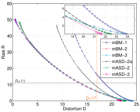
Using simulations, we consider the performance of the (255,239) RS code over an AWGN channel with BPSK as the modulation format. The mBM-1 curve corresponds to standard error-and-erasure BM decoding with multiple erasure patterns. For $l>1$, the mBM-$l$ curves correspond to error-and-erasure BM decoding with multiple decoding trials using both erasures and top-$l$ symbols. The mASD-$m$ curves correspond to multiple ASD decoding trials with maximum multiplicity $m$. The number of trial decoding patterns is $2^{R}$ where $R$ is denoted in parentheses in each algorithmโ€™s acronym (e.g., m-BM-2(11) uses $R=11$).

Fig. 2 shows the R-D curves for various algorithms atย Eb/No=5.2subscript๐ธ๐‘subscript๐‘๐‘œ5.2E_{b}/N_{o}=5.2ย dB. For this code, the fixed threshold for decoding is $D=n-k+1=17$. Therefore, one might expect that algorithms whose average distortion is less than 17 should have a frame error rate (FER) less than $\frac{1}{2}$. The R-D curve allows one to estimate the number of decoding patterns required to achieve this FER. Conventional BM decoding is very similar to mBM-1 decoding at rate 0. Notice that the mBM-1 algorithm at rate 0, which is very similar to conventional BM decoding, has an expected distortion of roughly 24. For this reason, the FER on conventional decoding is close to 1. The R-D curve tells us that trying roughly $2^{16}$ (i.e., $R=16$) erasure patterns would reduce the FER to roughly $\frac{1}{2}$ because this is where the distortion drops down to 17. Likewise, the mBM-2(11) algorithm has an expected distortion of less than 14. So we expect (and our simulations confirm) that the FER should be less than $\frac{1}{2}$. One weakness of this approach is that the R-D describes only the average distortion and does not directly consider the probability that the distortion is greater than 17. Still, we can make the following observations from the R-D curve. Even at low rates (e.g., $R\geq 4$), we see that the distortionย D๐ทDย achieved by mBM-2 is roughly the same as mBM-3, mASD-2, and mASD-3 but smaller than mASD-2a and mBM-1. This implies that mBM-2 is no worse than the more complicated ASD based approaches for a wide range of rates (i.e., $4\leq R\leq 35$).

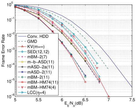
The FER of various algorithms can be seen in Fig. 2. The focus on $R=11$ allows us to make fair comparisons with SED(12,12). With the same number of decoding trials, mBM-2(11) outperforms SED(12,12) by 0.3 dB at an FER$=10^{-4}$. Even mBM-2(7), with many fewer decoding trials, outperforms both SED(12,12) and the KV algorithm withย m=โˆž๐‘šm=\infty. Among all our proposed algorithms with rateย R=11๐‘…11R=11, the mBM-HM74(11) achieves the best performance. This algorithm uses the Hamming (7,4) covering code for the 7 LRPs and the R-D approach for the remaining codeword positions. Meanwhile, small differences in the performance between mBM-2(11), mBM-3(11), mASD-2(11), and mASD-3(11) suggest that: (i) taking care of theย 222ย most likely symbols at each codeword position is good enough for multiple decoding of high-rate RS code and (ii) multiple runs of error-and-erasure decoding is almost as good as multiple runs of ASD decoding. Recall that this result is also correctly predicted by the R-D analysis. Moreover, it is quite reasonable since we know that the gain of GS decoding, with infinite multiplicity, over the BM algorithm is negligible for high-rate RS codes. To compare with the LCC($\eta=4$) Chase-type approach used in [7], we also consider the mBM-HM74(4) algorithm, which uses the Hamming (7,4) covering codes for the 7 LRPs and the hard decision pattern for the remaining codeword positions. This shows that the covering code achieves better performance with the same number ($2^{4}$) decoding attempts. The comparison is not entirely fair, however, because of their low-complexity approach to multiple decoding. We believe, nevertheless, that their technique can be generalized to covering codes.

VII Conclusion

A rate-distortion approach is proposed as a unified framework to analyze multiple decoding trials, with various algorithms, of RS codes in terms of performance and complexity. A connection is made between the complexity and performance (in some asymptotic sense) of these multiple-decoding algorithms and the rate and distortion of an associated R-D problem. Covering codes are also combined with the rate-distortion approach to mitigate the suboptimality of random codes when the effective block-length is not large. As part of this analysis, we also present numerical and analytical computations of the rate-distortion function for sequences of independent but non-identical sources. Finally, the simulation results show that our proposed algorithms based on the R-D approach achieve a better performance-versus-complexity trade-off than previously proposed algorithms. One key result is that, for high-rate RS codes, multiple-decoding using the standard BM algorithm is as good as multiple-decoding using more complex ASD algorithms.

In this paper, we only discuss the rate-distortion approach to solve the problem in (3). However, the performance can be further improved by focusing on the rate-distortion error-exponent. This allows us to approximately solve the covering problem for finiteย n๐‘›n rather than just asย nโ†’โˆžโ†’๐‘›n\rightarrow\infty. The complexity of multiple decoding can also be decreased by using clever techniques to lower the complexity per decoding trial (e.g., [7]). We will address these two improvements in a future paper.

Appendix A Proof of Theorem 2

First, let us recall that for each source componentย xisubscript๐‘ฅ๐‘–x_{i}, the B-A algorithm computes the R-D pair in the following steps:

  1. 1.

    Choose an arbitrary all-positive test-channel input-probability distribution vectorย qยฏ(0)superscriptยฏ๐‘ž0\underline{q}^{(0)}.

  2. 2.

    Iterate the following steps atย t=1,2,โ€ฆ๐‘ก12โ€ฆt=1,2,\ldots

    Qki|ji(t)=qki(t)โ€‹expโก(sโ€‹ฮดjiโ€‹ki)โˆ‘kiqki(t)โ€‹expโก(sโ€‹ฮดjiโ€‹ki)โ€‹andย โ€‹โˆ‘jipjiโ€‹Qkj|ji(t)=qki(t+1)superscriptsubscript๐‘„conditionalsubscript๐‘˜๐‘–subscript๐‘—๐‘–๐‘กsuperscriptsubscript๐‘žsubscript๐‘˜๐‘–๐‘ก๐‘ subscript๐›ฟsubscript๐‘—๐‘–subscript๐‘˜๐‘–subscriptsubscript๐‘˜๐‘–superscriptsubscript๐‘žsubscript๐‘˜๐‘–๐‘ก๐‘ subscript๐›ฟsubscript๐‘—๐‘–subscript๐‘˜๐‘–andย subscriptsubscript๐‘—๐‘–subscript๐‘subscript๐‘—๐‘–superscriptsubscript๐‘„conditionalsubscript๐‘˜๐‘—subscript๐‘—๐‘–๐‘กsuperscriptsubscript๐‘žsubscript๐‘˜๐‘–๐‘ก1Q_{k_{i}|j_{i}}^{(t)}=\frac{q_{k_{i}}^{(t)}\exp(s\delta_{j_{i}k_{i}})}{\sum_{k_{i}}q_{k_{i}}^{(t)}\exp(s\delta_{j_{i}k_{i}})}\,\,\,\mbox{and$\,\,\,$}\sum_{j_{i}}p_{j_{i}}Q_{k_{j}|j_{i}}^{(t)}=q_{k_{i}}^{(t+1)}

    whereย Qki|ji=Prโก(x^i=ki|xi=ji)subscript๐‘„conditionalsubscript๐‘˜๐‘–subscript๐‘—๐‘–Prsubscript^๐‘ฅ๐‘–conditionalsubscript๐‘˜๐‘–subscript๐‘ฅ๐‘–subscript๐‘—๐‘–Q_{k_{i}|j_{i}}=\Pr(\hat{x}_{i}=k_{i}|x_{i}=j_{i})ย is the transition probability. It is shown by B-A thatย qki(t)โ†’qkiโ‹†โ†’superscriptsubscript๐‘žsubscript๐‘˜๐‘–๐‘กsuperscriptsubscript๐‘žsubscript๐‘˜๐‘–โ‹†q_{k_{i}}^{(t)}\rightarrow q_{k_{i}}^{\star}ย andย Qki|ji(t)โ†’Qki|jiโ‹†โ†’superscriptsubscript๐‘„conditionalsubscript๐‘˜๐‘–subscript๐‘—๐‘–๐‘กsuperscriptsubscript๐‘„conditionalsubscript๐‘˜๐‘–subscript๐‘—๐‘–โ‹†Q_{k_{i}|j_{i}}^{(t)}\rightarrow Q_{k_{i}|j_{i}}^{\star}asย tโ†’โˆžโ†’๐‘กt\rightarrow\infty.

The rate and distortion can be computed byย Ri,s=โˆ‘jiโˆ‘kipjiโ€‹Qki|jiโ‹†โ€‹logโกQki|jiโ‹†โˆ‘jipjiโ€‹Qki|jiโ‹†subscript๐‘…๐‘–๐‘ subscriptsubscript๐‘—๐‘–subscriptsubscript๐‘˜๐‘–subscript๐‘subscript๐‘—๐‘–superscriptsubscript๐‘„conditionalsubscript๐‘˜๐‘–subscript๐‘—๐‘–โ‹†superscriptsubscript๐‘„conditionalsubscript๐‘˜๐‘–subscript๐‘—๐‘–โ‹†subscriptsubscript๐‘—๐‘–subscript๐‘subscript๐‘—๐‘–superscriptsubscript๐‘„conditionalsubscript๐‘˜๐‘–subscript๐‘—๐‘–โ‹†R_{i,s}=\sum_{j_{i}}\sum_{k_{i}}p_{j_{i}}Q_{k_{i}|j_{i}}^{\star}\log\frac{Q_{k_{i}|j_{i}}^{\star}}{\sum_{j_{i}}p_{j_{i}}Q_{k_{i}|j_{i}}^{\star}}ย andย โˆ‘i=1nDi,s=โˆ‘jiโˆ‘kipjiโ€‹Qki|jiโ‹†โ€‹ฯjiโ€‹kisuperscriptsubscript๐‘–1๐‘›subscript๐ท๐‘–๐‘ subscriptsubscript๐‘—๐‘–subscriptsubscript๐‘˜๐‘–subscript๐‘subscript๐‘—๐‘–superscriptsubscript๐‘„conditionalsubscript๐‘˜๐‘–subscript๐‘—๐‘–โ‹†subscript๐œŒsubscript๐‘—๐‘–subscript๐‘˜๐‘–\sum_{i=1}^{n}D_{i,s}=\sum_{j_{i}}\sum_{k_{i}}p_{j_{i}}Q_{k_{i}|j_{i}}^{\star}\rho_{j_{i}k_{i}}

Now, we will prove Theorem 2. Since the input-distribution vector of the test channel is an arbitrary all-positive vector, we chooseย qK(0)superscriptsubscript๐‘ž๐พ0q_{K}^{(0)}ย so that it can be factorized as followsย qK(0)=โˆi=1nqki(0)superscriptsubscript๐‘ž๐พ0superscriptsubscriptproduct๐‘–1๐‘›superscriptsubscript๐‘žsubscript๐‘˜๐‘–0q_{K}^{(0)}=\prod_{i=1}^{n}q_{k_{i}}^{(0)} .

Suppose after stepย t๐‘กt, we haveย qK(t)=โˆi=1nqki(t)superscriptsubscript๐‘ž๐พ๐‘กsuperscriptsubscriptproduct๐‘–1๐‘›superscriptsubscript๐‘žsubscript๐‘˜๐‘–๐‘กq_{K}^{(t)}=\prod_{i=1}^{n}q_{k_{i}}^{(t)}ย then by the iterative computing process in the B-A algorithm we have

QK|J(t)=qK(t)โ€‹expโก(sโ€‹ฮดJโ€‹K)โˆ‘KqK(t)โ€‹expโก(sโ€‹ฮดJโ€‹K)=โˆi=1nqki(t)โ€‹expโก(sโ€‹ฮดjiโ€‹ki)โˆ‘k1โ€ฆโ€‹โˆ‘knโˆi=1nqki(t)โ€‹expโก(sโ€‹ฮดjiโ€‹ki)=โˆi=1nqki(t)โ€‹expโก(sโ€‹ฮดjiโ€‹ki)โˆ‘kiqki(t)โ€‹expโก(sโ€‹ฮดjiโ€‹ki)=โˆi=1nQki|ji(t)superscriptsubscript๐‘„conditional๐พ๐ฝ๐‘กsuperscriptsubscript๐‘ž๐พ๐‘ก๐‘ subscript๐›ฟ๐ฝ๐พsubscript๐พsuperscriptsubscript๐‘ž๐พ๐‘ก๐‘ subscript๐›ฟ๐ฝ๐พsuperscriptsubscriptproduct๐‘–1๐‘›superscriptsubscript๐‘žsubscript๐‘˜๐‘–๐‘ก๐‘ subscript๐›ฟsubscript๐‘—๐‘–subscript๐‘˜๐‘–subscriptsubscript๐‘˜1โ€ฆsubscriptsubscript๐‘˜๐‘›superscriptsubscriptproduct๐‘–1๐‘›superscriptsubscript๐‘žsubscript๐‘˜๐‘–๐‘ก๐‘ subscript๐›ฟsubscript๐‘—๐‘–subscript๐‘˜๐‘–superscriptsubscriptproduct๐‘–1๐‘›superscriptsubscript๐‘žsubscript๐‘˜๐‘–๐‘ก๐‘ subscript๐›ฟsubscript๐‘—๐‘–subscript๐‘˜๐‘–subscriptsubscript๐‘˜๐‘–superscriptsubscript๐‘žsubscript๐‘˜๐‘–๐‘ก๐‘ subscript๐›ฟsubscript๐‘—๐‘–subscript๐‘˜๐‘–superscriptsubscriptproduct๐‘–1๐‘›superscriptsubscript๐‘„conditionalsubscript๐‘˜๐‘–subscript๐‘—๐‘–๐‘กQ_{K|J}^{(t)}=\frac{q_{K}^{(t)}\exp(s\delta_{JK})}{\sum_{K}q_{K}^{(t)}\exp(s\delta_{JK})}=\frac{\prod_{i=1}^{n}q_{k_{i}}^{(t)}\exp(s\delta_{j_{i}k_{i}})}{\sum_{k_{1}}\ldots\sum_{k_{n}}\prod_{i=1}^{n}q_{k_{i}}^{(t)}\exp(s\delta_{j_{i}k_{i}})}=\prod_{i=1}^{n}\frac{q_{k_{i}}^{(t)}\exp(s\delta_{j_{i}k_{i}})}{\sum_{k_{i}}q_{k_{i}}^{(t)}\exp(s\delta_{j_{i}k_{i}})}=\prod_{i=1}^{n}Q_{k_{i}|j_{i}}^{(t)}
$$q_{K}^{(t+1)}=\sum_{J}p_{J}Q_{K|J}^{(t)}=\sum_{j_{1}}\ldots\sum_{j_{n}}\prod_{i=1}^{n}p_{j_{i}}Q_{k_{i}|j_{i}}^{(t)}=\prod_{i=1}^{n}\sum_{j_{i}}p_{j_{i}}Q_{k_{j}|j_{i}}^{(t)}=\prod_{i=1}^{n}q_{k_{i}}^{(t+1)}$$

whereย pJ=Prโก(xn=J)=โˆi=1nPrโก(xi=ji)=โˆi=1npjisubscript๐‘๐ฝPrsuperscript๐‘ฅ๐‘›๐ฝsuperscriptsubscriptproduct๐‘–1๐‘›Prsubscript๐‘ฅ๐‘–subscript๐‘—๐‘–superscriptsubscriptproduct๐‘–1๐‘›subscript๐‘subscript๐‘—๐‘–p_{J}=\Pr(x^{n}=J)=\prod_{i=1}^{n}\Pr(x_{i}=j_{i})=\prod_{i=1}^{n}p_{j_{i}}ย follows from the independence of source components.

Hence, by induction we know the factorization rule still applies after every stepย t๐‘กtย in the process. Therefore, we have

$$q_{K}^{\star}=\lim_{t\rightarrow\infty}q_{K}^{(t)}=\lim_{t\rightarrow\infty}\prod_{i=1}^{n}q_{k_{i}}^{(t)}=\prod_{i=1}^{n}\lim_{t\rightarrow\infty}q_{k_{i}}^{(t)}=\prod_{i=1}^{n}q_{k_{i}}^{\star}\,\,\mbox{$\,\,$ and}\,\,\,\,Q_{K|J}^{\star}=\lim_{t\rightarrow\infty}Q_{K|J}^{(t)}=\lim_{t\rightarrow\infty}\prod_{i=1}^{n}Q_{k_{i}|j_{i}}^{(t)}=\prod_{i=1}^{n}\lim_{t\rightarrow\infty}Q_{k_{i}|j_{i}}^{(t)}=\prod_{i=1}^{n}Q_{k_{i}|j_{i}}^{\star}$$

and then we can show that

Rs=โˆ‘Jโˆ‘KpJโ€‹QK|Jโ‹†โ€‹logโกQK|Jโ‹†โˆ‘JpJโ€‹QK|Jโ‹†=โˆ‘j1,โ€ฆ,jnโˆ‘k1,โ€ฆ,knโˆi=1npjiโ€‹Qki|jiโ‹†โ€‹โˆ‘i=1nlogโกQki|jiโ‹†โˆ‘jipjiโ€‹Qki|jiโ‹†=โˆ‘i=1nโˆ‘jiโˆ‘kipjiโ€‹Qki|jiโ‹†โ€‹logโกQki|jiโ‹†โˆ‘jipjiโ€‹Qki|jiโ‹†=โˆ‘i=1nRi,ssubscript๐‘…๐‘ subscript๐ฝsubscript๐พsubscript๐‘๐ฝsuperscriptsubscript๐‘„conditional๐พ๐ฝโ‹†superscriptsubscript๐‘„conditional๐พ๐ฝโ‹†subscript๐ฝsubscript๐‘๐ฝsuperscriptsubscript๐‘„conditional๐พ๐ฝโ‹†subscriptsubscript๐‘—1โ€ฆsubscript๐‘—๐‘›subscriptsubscript๐‘˜1โ€ฆsubscript๐‘˜๐‘›superscriptsubscriptproduct๐‘–1๐‘›subscript๐‘subscript๐‘—๐‘–superscriptsubscript๐‘„conditionalsubscript๐‘˜๐‘–subscript๐‘—๐‘–โ‹†superscriptsubscript๐‘–1๐‘›superscriptsubscript๐‘„conditionalsubscript๐‘˜๐‘–subscript๐‘—๐‘–โ‹†subscriptsubscript๐‘—๐‘–subscript๐‘subscript๐‘—๐‘–superscriptsubscript๐‘„conditionalsubscript๐‘˜๐‘–subscript๐‘—๐‘–โ‹†superscriptsubscript๐‘–1๐‘›subscriptsubscript๐‘—๐‘–subscriptsubscript๐‘˜๐‘–subscript๐‘subscript๐‘—๐‘–superscriptsubscript๐‘„conditionalsubscript๐‘˜๐‘–subscript๐‘—๐‘–โ‹†superscriptsubscript๐‘„conditionalsubscript๐‘˜๐‘–subscript๐‘—๐‘–โ‹†subscriptsubscript๐‘—๐‘–subscript๐‘subscript๐‘—๐‘–superscriptsubscript๐‘„conditionalsubscript๐‘˜๐‘–subscript๐‘—๐‘–โ‹†superscriptsubscript๐‘–1๐‘›subscript๐‘…๐‘–๐‘ R_{s}=\sum_{J}\sum_{K}p_{J}Q_{K|J}^{\star}\log\frac{Q_{K|J}^{\star}}{\sum_{J}p_{J}Q_{K|J}^{\star}}=\sum_{j_{1},\ldots,j_{n}}\sum_{k_{1},\ldots,k_{n}}\prod_{i=1}^{n}p_{j_{i}}Q_{k_{i}|j_{i}}^{\star}\sum_{i=1}^{n}\log\frac{Q_{k_{i}|j_{i}}^{\star}}{\sum_{j_{i}}p_{j_{i}}Q_{k_{i}|j_{i}}^{\star}}=\sum_{i=1}^{n}\sum_{j_{i}}\sum_{k_{i}}p_{j_{i}}Q_{k_{i}|j_{i}}^{\star}\log\frac{Q_{k_{i}|j_{i}}^{\star}}{\sum_{j_{i}}p_{j_{i}}Q_{k_{i}|j_{i}}^{\star}}=\sum_{i=1}^{n}R_{i,s}
Ds=โˆ‘Jโˆ‘KpJโ€‹QK|Jโ‹†โ€‹ฯJโ€‹K=โˆ‘j1,โ€ฆ,jnโˆ‘k1,โ€ฆ,knโˆi=1npjiโ€‹Qki|jiโ‹†โ€‹โˆ‘i=1nฯjiโ€‹ki=โˆ‘i=1nโˆ‘jiโˆ‘kipjiโ€‹Qki|jiโ‹†โ€‹ฯjiโ€‹ki=โˆ‘i=1nDi,s.subscript๐ท๐‘ subscript๐ฝsubscript๐พsubscript๐‘๐ฝsuperscriptsubscript๐‘„conditional๐พ๐ฝโ‹†subscript๐œŒ๐ฝ๐พsubscriptsubscript๐‘—1โ€ฆsubscript๐‘—๐‘›subscriptsubscript๐‘˜1โ€ฆsubscript๐‘˜๐‘›superscriptsubscriptproduct๐‘–1๐‘›subscript๐‘subscript๐‘—๐‘–superscriptsubscript๐‘„conditionalsubscript๐‘˜๐‘–subscript๐‘—๐‘–โ‹†superscriptsubscript๐‘–1๐‘›subscript๐œŒsubscript๐‘—๐‘–subscript๐‘˜๐‘–superscriptsubscript๐‘–1๐‘›subscriptsubscript๐‘—๐‘–subscriptsubscript๐‘˜๐‘–subscript๐‘subscript๐‘—๐‘–superscriptsubscript๐‘„conditionalsubscript๐‘˜๐‘–subscript๐‘—๐‘–โ‹†subscript๐œŒsubscript๐‘—๐‘–subscript๐‘˜๐‘–superscriptsubscript๐‘–1๐‘›subscript๐ท๐‘–๐‘ D_{s}=\sum_{J}\sum_{K}p_{J}Q_{K|J}^{\star}\rho_{JK}=\sum_{j_{1},\ldots,j_{n}}\sum_{k_{1},\ldots,k_{n}}\prod_{i=1}^{n}p_{j_{i}}Q_{k_{i}|j_{i}}^{\star}\sum_{i=1}^{n}\rho_{j_{i}k_{i}}=\sum_{i=1}^{n}\sum_{j_{i}}\sum_{k_{i}}p_{j_{i}}Q_{k_{i}|j_{i}}^{\star}\rho_{j_{i}k_{i}}=\sum_{i=1}^{n}D_{i,s}.

References

  • [1] V.ย Guruswami and M.ย Sudan, โ€œImproved decoding of Reed-Solomon and Algebraic-Geometry codes,โ€ IEEE Trans. Inform. Theory, vol.ย 45, no.ย 6, pp. 1757โ€“1767, Sept. 1998.
  • [2] R.ย Koetter and A.ย Vardy, โ€œAlgebraic soft-decision decoding of Reed-Solomon codes,โ€ IEEE Trans. Inform. Theory, vol.ย 49, no.ย 11, pp. 2809โ€“2825, Nov. 2003.
  • [3] G.ย D. Forney, โ€œGeneralized minimun distance decoding,โ€ IEEE Trans. Inform. Theory, vol.ย 12, no.ย 2, pp. 125โ€“131, April 1966.
  • [4] S.ย -W. Lee and B.ย V.ย K.ย V. Kumar, โ€œSoft-decision decoding of Reed-Solomon codes using successive error-and-erasure decoding,โ€ in Proc. IEEE Global Telecom. Conf., New Orleans, LA, Nov. 2008, pp. 1โ€“5.
  • [5] D.ย Chase, โ€œA class of algorithms for decoding block codes with channel measurement information,โ€ IEEE Trans. Inform. Theory, vol.ย 18, no.ย 1, pp. 170โ€“182, Jan. 1972.
  • [6] M.ย F.ย H. Tang, Y.ย Liu and S.ย Lin, โ€œOn combining Chase-2 and GMD decoding algorithms for nonbinary block codes,โ€ IEEE Commun. Letters, vol.ย 5, no.ย 5, pp. 209โ€“211, May 2001.
  • [7] J.ย Bellorado and A.ย Kavฤiฤ‡, โ€œA low-complexity method for Chase-type decoding of Reed-Solomon codes,โ€ in Proc. IEEE Int. Symp. Information Theory, Seattle, USA, 2006, pp. 2037โ€“2041.
  • [8] H.ย Xia and J.ย R. Cruz, โ€œReliability-based forward recursive algorithms for algebraic soft-decision decoding of Reed-Solomon codes,โ€ IEEE Trans. Commun., vol.ย 55, no.ย 7, pp. 1273โ€“1278, 2007.
  • [9] H.ย Xia, H.ย Wang, and J.ย R. Cruz, โ€œA Chase-GMD algorithm for soft-decision decoding of Reed-Solomon codes on perpendicular channels,โ€ in Proc. IEEE Int. Conf. Commun., Beijing, China, May 2008, pp. 1977โ€“1981.
  • [10] S.ย Lin and D.ย J. Costello, Jr., Error Control Coding: Fundamentals and Applications. Englewood Cliffs, NJ, USA: Prentice Hall, 1983, iSBN 0-13-283796-X.
  • [11] R.ย E. Blahut, Algebraic Codes for Data Transmission. Cambridge University Press, 2003, iSBN-10 0521553741.
  • [12] โ€”โ€”, โ€œComputation of channel capacity and rate distortion functionsโ€ IEEE Trans. Inform. Theory, vol.ย 18, no.ย 4, pp. 460โ€“473, July 1972.
  • [13] S.ย Arimoto, โ€œAn algorithm for computing the capacity of arbitrary discrete memoryless channels,โ€ IEEE Trans. Inform. Theory, vol.ย 18, no.ย 1, pp. 14โ€“20, Jan. 1972.
  • [14] J.ย Jiang and K.ย R. Narayanan, โ€œAlgebraic soft-decision decoding of Reed-Solomon codes using bit-level soft information,โ€ IEEE Trans. Inform. Theory, vol.ย 54, no.ย 9, pp. 3907โ€“3928, Sept. 2008.
  • [15] R.ย J. McEliece, โ€œThe Guruswami-Sudan decoding algorithm for Reed-Solomon codes,โ€ JPL Interplanetary Network Progress Report, pp. 42โ€“153, May 2003.
  • [16] P.ย S. Nguyen, H.ย D. Pfister and K.ย R. Narayanan, โ€œOn multiple decoding attempts for Reed-Solomon codes,โ€ 2009, in preparation.
  • [17] T.ย Berger, Rate Distortion Theory. Englewood Cliffs, NJ, USA: Prentice Hall, Inc., 1971, iSBN 13-753103-6.
  • [18] T.ย M. Cover and J.ย A. Thomas, Elements of Infomation Theory. Wiley, 1991.