The spin evolution of spin-3 ⁵²Cr Bose-Einstein condensate

Abstract

The spin evolution of a Bose-Einstein condensate starting from a mixture of two or three groups of ⁵²Cr (spin-$3$) atoms in an optical trap has been studied theoretically. The initial state is so chosen that the system does not distinguish up and down. In this choice, the deviation caused by the single-mode approximation is reduced. Moreover, since the particle number is given very small ($N=20$), the deviation caused by the neglect of the long-range dipole force is also reduced. Making use of these two simplifications, a theoretical calculation beyond the mean field theory is performed. The numerical results are help to evaluate the unknown strength $g_{0}$.

I Introduction

Bose-Einstein condensate (BEC) of atoms with nonzero spin has greatly attracted the interest of both the experimentalists and theorists HTL1998 ; OT1998 ; SDM1998 ; SJ1998 ; LCK1998 ; GA2003 ; LM2007 in recent years. Four years ago, the Bose gas of ⁵²Cr atoms with electronic spin $J=3$ and nuclear spin $I=0$ was condensed successfully GA2005 . Experimentally, the atomic spins of ⁵²Cr were frozen in magnetic trap, but freed in optical trap DBR2006 . For these spin-3 bosons, the interaction between two atoms is specified by the strengths $g_{S}$, where $S=0$, $2$, $4$ and $6$ are the total spins of the pair. All $g_{S}$ except the one for $S=0$ have been determined experimentally SJ2005 . To fully understand the characteristic of ⁵²Cr and consider the use of this material in application, it is important to measure $g_{0}$ with the help of theory. Among all the rich physics of BEC, one attractive phenomenon is the spin evolution LCK1998 ; SH2004 ; CMS2004 ; CMS2005 ; PH1999 ; DRB2006 . It was found that for ⁸⁷Rb and ²³Na, the evolution of the average populations of spin components sensitively depends on the strengths of interaction LMA2007 ; CZF2008 . Therefore, the interaction can be determined (or confirmed) by observing the evolution. However, for ⁵²Cr, related experimental data and theoretical analysis are scarce.

In this paper, we consider the spin evolution of a mixture of two or three groups of ⁵²Cr atoms in an optical trap. Each atom of a group has the same $Z$ component of spin, $\mu$. Magnetic fields are used in the preparation of these groups, but are cancelled during the whole evolution. What we are interesting in is the effect of the unknown strength $g_{0}$ on the evolution. When the condensate is very dilute and the temperature is very low, the single-mode approximation (SMA, namely, the spatial wave functions of the atoms distinct in $\mu$ are approximately considered as the same) has been used by a number of authors to simplify the calculation. This approximation has also been adopted here. However, even the above conditions are satisfied, the SMA might not be good as shown in YS2002 . The validity of the SMA depends on the total magnetization of the system. In the following discussion, a special initial condition with total magnetization zero is chosen. Accordingly, the system does not distinguish up and down. Therefore, the deviation caused by the SMA is expected to be considerably reduced.

It is well known that the system of ⁵²Cr contains the long-range dipole interaction which is considerably stronger than those of ⁸⁷Rb and ²³Na. The dipole interaction is in general very weak. However, due to being long-range, the combined effect would be large if numerous atoms are involved. Besides, the effect would become larger and larger as the evolution goes on. Accordingly, we consider only the condensate with much fewer particles and the early stage of evolution. For this very small condensate, the effect of dipole force is much smaller and therefore can be neglected. Furthermore, since the particle number $N$ under consideration is so small, the mean field theory might not work very well. Thus a method beyond the mean field theory is used in the follows.

II Hamiltonian and the eigenstates

For a ⁵²Cr condensate with $N$ atoms, when the dipole force is neglected, the interaction between a pair of spin-3 bosons $i$ and $j$ is denoted as $U_{ij}=O_{ij}\delta(\vec{\mathbf{r}}_{i}-\vec{\mathbf{r}}_{j})$, where $O_{ij}=g_{0}P_{0}+g_{2}P_{2}+g_{4}P_{4}+g_{6}P_{6}$. And $P_{0}$ to $P_{6}$ are the projection operators of the $S$-channels. Based on the SMA, each boson has the same spatial state $\phi(\vec{\mathbf{r}}_{k})$. When integration over the spatial degrees of freedom has been performed, the Hamiltonian reads

$$H=\sum_{i<j}U_{ij}=f\sum_{i<j}O_{ij},\ \ \ f=\int|\phi(\vec{\mathbf{r}})|^{4}d\vec{\mathbf{r}}.$$ (1)

After the integration, only the spin degrees of freedom are left in the Hamiltonian. To diagonalize the Hamiltonian, we use the following Fock-states as the basis functions

$$|\alpha\rangle=|N_{\bar{3}}N_{\bar{2}}N_{\bar{1}}N_{0}N_{1}N_{2}N_{3}\rangle,$$ (2)

where $\alpha$ indicates the set $\{N_{\bar{3}},\cdots,N_{3}\}$, $N_{\mu}$ is the number of bosons with spin component $\mu$, and $\bar{\mu}$ means $-\mu$. There exist two restrictions on the $N_{\mu}$ as follows.

$$\left\{\begin{array}[]{lll}N&=&N_{\bar{3}}+N_{\bar{2}}+N_{\bar{1}}+N_{0}+N_{1}+N_{2}+N_{3}\\ M&=&-3N_{\bar{3}}-2N_{\bar{2}}-N_{\bar{1}}+N_{1}+2N_{2}+3N_{3}\end{array}\right.,$$ (3)

where $M$ is the total magnetization (a constant). In the Fock space, by using the factional parentage coefficient BCG2004 , the matrix elements of Hamiltonian read

$$\langle\beta|H|\alpha\rangle = \langle N^{\prime}_{\bar{3}}N^{\prime}_{\bar{2}}N^{\prime}_{\bar{1}}N^{\prime}_{0}N^{\prime}_{1}N^{\prime}_{2}N^{\prime}_{3}|f\sum_{i<j}O_{ij}|N_{\bar{3}}N_{\bar{2}}N_{\bar{1}}N_{0}N_{1}N_{2}N_{3}\rangle$$ (4)

$$= 2f\sum_{\mu\leq\nu;\mu^{\prime}\leq\nu^{\prime}}\delta_{\mu^{\prime}+\nu^{\prime},\mu+\nu}\sum_{S=0,2,4,6}g_{S}C_{3\mu^{\prime},3\nu^{\prime}}^{S,(\mu^{\prime}+\nu^{\prime})}C_{3\mu,3\nu}^{S,(\mu+\nu)}$$

$$[\ \delta_{\mu^{\prime}\nu^{\prime}}\delta_{\mu\nu}\frac{N_{\mu}(N_{\mu}-1)}{4}\delta_{\cdots,N_{\mu}-2,\cdots}^{\cdots,N^{\prime}_{\mu}-2,\cdots}$$

$$+(1-\delta_{\mu^{\prime}\nu^{\prime}})\delta_{\mu\nu}\frac{\sqrt{N^{\prime}_{\mu^{\prime}}N^{\prime}_{\nu^{\prime}}N_{\mu}(N_{\mu}-1)}}{2}\delta_{\cdots,N_{\mu}-2,\cdots}^{\cdots,N^{\prime}_{\mu^{\prime}}-1,\cdots,N^{\prime}_{\nu^{\prime}}-1,\cdots}$$

$$+(1-\delta_{\mu\nu})\delta_{\mu^{\prime}\nu^{\prime}}\frac{\sqrt{N_{\mu}N_{\nu}N^{\prime}_{\mu^{\prime}}(N^{\prime}_{\mu^{\prime}}-1)}}{2}\delta_{\cdots,N_{\mu}-1,\cdots,N_{\nu}-1,\cdots}^{\cdots,N^{\prime}_{\mu^{\prime}}-2,\cdots}$$

$$+(1-\delta_{\mu\nu})(1-\delta_{\mu^{\prime}\nu^{\prime}})\sqrt{N_{\mu}N_{\nu}N^{\prime}_{\mu^{\prime}}N^{\prime}_{\nu^{\prime}}}\delta_{\cdots,N_{\mu}-1,\cdots,N_{\nu}-1,\cdots}^{\cdots,N^{\prime}_{\mu^{\prime}}-1,\cdots,N^{\prime}_{\nu^{\prime}}-1,\cdots}\ ],$$

where $C_{3\mu,3\nu}^{S,(\mu+\nu)}$ is the Clebsch-Gordan coefficient. In the label $\delta_{\cdots,N_{\mu}-2,\cdots}^{\cdots,N^{\prime}_{\mu^{\prime}}-1,\cdots,N^{\prime}_{\nu^{\prime}}-1,\cdots}$, the superscript denotes a revised set of $\{N^{\prime}_{\bar{3}},\cdots,N^{\prime}_{3}\}$ by reducing both $N^{\prime}_{\mu^{\prime}}$ and $N^{\prime}_{\nu^{\prime}}$ by 1, and the subscript denotes a revised set of $\{N_{\bar{3}},\cdots,N_{3}\}$ by reducing $N_{\mu}$ by $2$. When the two revised sets are one-to-one identical, the label is $1$, otherwise it is zero.

When both $N$ and $M$ are given, the dimension of the matrix is finite. After the Hamiltonian is diagonalized, the $j$-th eigenenergy $E_{j}$ and the corresponding eigenstate $\psi_{j}$ are obtained. $\psi_{j}$ can be expanded by the basis functions (or vice versa) as follows.

$$\psi_{j}=\sum_{\alpha}c_{\alpha}^{j}|\alpha\rangle\ \ \ \mbox{or}\ \ \ |\alpha\rangle=\sum_{j}c_{\alpha}^{j}\psi_{j},$$ (5)

where the coefficient $c_{\alpha}^{j}=\langle\alpha|\psi_{j}\rangle$ is real. These eigenstates are used in the following description of evolution.

III Evolution of population of spin components

The spin evolution begins when the three groups of atoms are mixed together. All the atoms of the first group have $\mu=3$, those of the second have $\mu=-3$ and those of the third have $\mu=0$. Therefore, the initial state is just a Fock-state $|I\rangle=|N_{\bar{3}},0,0,N_{0},0,0,N_{3}\rangle$, where $N_{3}$, $N_{\bar{3}}$, and $N_{0}$ are the number of atoms in the first to third groups, respectively. $|I\rangle$ can be expanded by the series of $\psi_{j}$ with the coefficients $c_{I}^{j}$. Thus the time-dependent solution of the Schrödinger equation $\Psi(t)$ describing the evolution reads

$$\Psi(t)=e^{-iHt/\hbar}|I\rangle=\sum_{j}c_{I}^{j}e^{-iE_{j}t/\hbar}\psi_{j}.$$ (6)

Since $c_{I}^{j}$ are known constants determined by $|I\rangle$, $E_{j}$ and $\psi_{j}$ are also known. So the evolution can be fully understood.

From $\Psi(t)$, we define the time-dependent population $P_{\mu}^{I}(t)$ which is the probability of an atom in spin component $\mu$ at $t$. It reads,

$$P_{\mu}^{I}(t)=\frac{1}{N}\langle\Psi(t)|a_{\mu}^{+}a_{\mu}|\Psi(t)\rangle=B_{\mu}^{I}+O_{\mu}^{I}(t)$$ (7)

where $a_{\mu}^{+}$ and $a_{\mu}$ are the creation operator and annihilation operator of an atom in $\mu$, respectively.

$$B_{\mu}^{I} = \sum_{j}(c_{I}^{j})^{2}\sum_{\alpha}(c_{\alpha}^{j})^{2}\frac{N_{\mu}^{\alpha}}{N}$$ (8)

$$O_{\mu}^{I}(t) = 2\sum_{j<j^{\prime}}\cos[\frac{(E_{j^{\prime}}-E_{j})t}{\hbar}]c_{I}^{j}c_{I}^{j^{\prime}}\sum_{\alpha}c_{\alpha}^{j}c_{\alpha}^{j^{\prime}}\frac{N_{\mu}^{\alpha}}{N}$$ (9)

$N_{\mu}^{\alpha}$ is the number of atoms in $\mu$ within $|\alpha\rangle$. Equation (7) contains two terms. The first one $B_{\mu}^{I}$ is only determined by $|I\rangle$ and is time-independent and therefore, appears as a background of oscillation. The second one $O_{\mu}^{I}(t)$ contains the time-dependent factor $\cos[(E_{j^{\prime}}-E_{j})t/\hbar]$ which implies an oscillation upon the above background. At the beginning of evolution (i.e., $t=0$), $\Psi(0)=|I\rangle$ and $P_{\mu}^{I}(0)=N_{\mu}^{I}/N$. Moreover, if the initial state has the symmetry $N_{\bar{\mu}}^{I}=N_{\mu}^{I}$, the population would also be symmetric where $P_{\bar{\mu}}^{I}(t)=P_{\mu}^{I}(t)$. This is because in this case, the $Z$ axis can be reversed.

In the following calculation, $N=20$ is given. The initial states are given as $N_{\pm 3}^{I}=(N-N_{0}^{I})/2$ and $N_{\pm 2}^{I}=N_{\pm 1}^{I}=0$, where $N_{0}^{I}$ is even and is ranged from $0$ to $N$. In this choice, $|I\rangle$ is uniquely determined by $N_{0}^{I}$. Obviously, the system has the up-down symmetry. And the total magnetization $M$ is zero, which is a condition in favor of the SMA. The $10^{-8}$ meV, ${\mathring{A}}$ and $\sec$ are used as units for energy, length and time, respectively. The strengths $g_{2}$, $g_{4}$ and $g_{6}$ are taken from WJ2005 , namely, they are $-3.88$, $30.80$ and $59.64,$ respectively, whereas $g_{0}$ will be given at a number of testing values. The average density is given as $f=2\times 10^{-11}$. This value is simply evaluated under a model that the density is uniform inside a sphere. A slight deviation of $f$ does not affect the following qualitative results.

III.1 The background $B_{\mu}^{I}$

It is proved that the background of oscillation in spin-evolutions of spin-1 condensates does not depend on the interaction LB2008 . However, the argument of that paper is based on the uniqueness of the Fock-state with a given $N$, $M$, and $N_{0}$. Obviously, the uniqueness holds no more for spin-3 systems. Therefore, the knowledge of interaction might generally be obtained by observing $B_{\mu}^{I}$. This is shown in Fig. 1 where the dependency on the initial state and on $g_{0}$ is revealed. It is also shown that $B_{\mu}^{I}$ would depend on $g_{0}$ rather weakly if $g_{0}$ is positive. In this case, the structures of low-lying eigenstates would be dominated by $S=2$ pairs (because only in this kind of pairs, the two atoms are mutually attracted). However, $B_{\mu}^{I}$ would depend on $g_{0}$ rather strongly if $g_{0}$ is negative and close to $g_{2}$. In this case, the structures of the eigenstates would vary sensitively with $g_{0}$ due to the competition of the $S=2$ and $S=0$ pairs BCG2009 . As a result, there is a domain of sensitivity. If the realistic $g_{0}$ turns out to fall in this domain, it could be determined by observing $B_{\mu}^{I}$.

The background can be rewritten as $B_{\mu}^{I}=\sum_{j}W_{j}^{I}Q_{\mu}^{j}$, where $W_{j}^{I}=(c_{I}^{j})^{2}$ is the weight of $\psi_{j}$ in $|I\rangle$, $Q_{\mu}^{j}=\sum_{\alpha}(c_{\alpha}^{j})^{2}N_{\mu}^{\alpha}/N\equiv\langle\psi_{j}|a_{\mu}^{+}a_{\mu}|\psi_{j}\rangle/N$ is the probability of an atom in $\mu$ within $\psi_{j}$. Note that the curve with $N_{0}^{I}=0$ is much higher in Fig. 1(a), but much lower in Fig. 1(d). In this state, all the spins are either up ($\mu=3$) or down ($\mu=-3$) initially. Therefore, those $\psi_{j}$ with a larger $Q_{\pm 3}^{j}$ (i.e., having averagely more atoms for $\mu=\pm 3$) would have a larger weight $W_{j}^{I}$. This fact explains why the curve with $N_{0}^{I}=0$ is the highest in Fig. 1(a), where the $\mu=3$ atoms are observed. Meanwhile, those $\psi_{j}$ with a larger $Q_{0}^{j}$ would have a smaller weight $W_{j}^{I}$, which explains why the curve with $N_{0}^{I}=0$ is the lowest in Fig. 1(d).

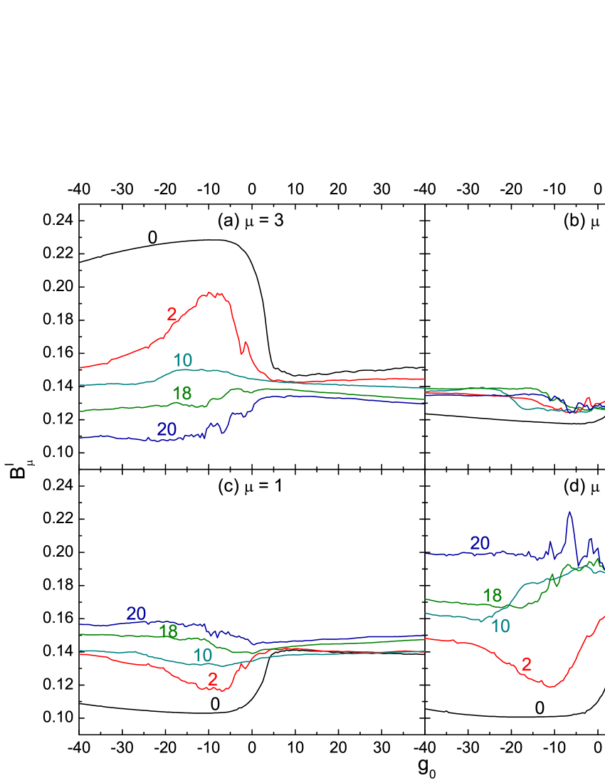
Figure 1: (Color online.) The background of spin evolution, $B^{I}_{\mu}$, against $g_{0}$ where (a) $\mu=3$, (b) $\mu=2$, (c) $\mu=1$ and (d) $\mu=0$, respectively. Five cases of initial states where $N_{0}^{I}=0$, $2$, $10$, $18$ and $20$, respectively, are given and marked by the curves.

III.2 The oscillation $O_{\mu}^{I}(t)$

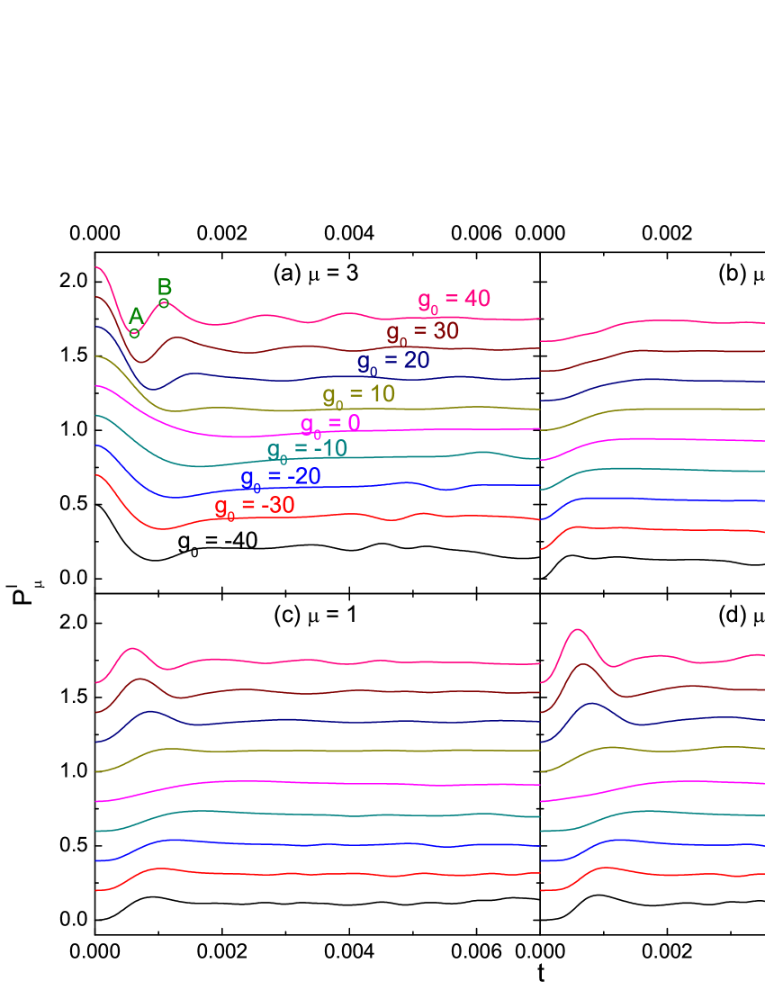
Figure 2: (Color online.) The populations of spin evolution, $P^{I}_{\mu}(t)$, against $t$ (in second) where (a) $\mu=3$, (b) $\mu=2$, (c) $\mu=1$ and (d) $\mu=0$, respectively. The initial state has $N_{0}^{I}=0$. In every subfigure, the curves from the lowest to the highest have $g_{0}$ from $-40$ to $40$ with a step $10$ as marked in (a). Each curve has been shifted upward by $0.2$ more than its lower adjacent to guide the eyes.

Table 1: The first minimum and the second maximum of $P^{I}_{3}(t)$ denoted as $P_{3,A}^{I}$ and $P_{3,B}^{I}$, respectively, for $N_{0}^{I}=0$. $T_{3,A}^{I}$ and $T_{3,B}^{I}$ are their locations (in ms).

$g_{0}$	$-40$	$-30$	$-20$	$-10$	$0$	$10$	$20$	$30$	$40$
$P_{3,A}^{I}$	$0.12$	$0.13$	$0.15$	$0.16$	$0.16$	$0.13$	$0.07$	$0.06$	$0.05$
$T_{3,A}^{I}$	$0.94$	$1.08$	$1.26$	$1.66$	$2.30$	$1.26$	$0.92$	$0.74$	$0.60$
$P_{3,B}^{I}$	$0.21$	$0.21$	$0.25$	$0.25$	$0.21$	$0.15$	$0.18$	$0.23$	$0.26$
$T_{3,B}^{I}$	$1.84$	$2.62$	$4.88$	$6.10$	$5.60$	$1.94$	$1.58$	$1.30$	$1.10$

In Eq. (8), the time factor $(E_{j^{\prime}}-E_{j})/\hbar$ is in general not a multiple of integer among all pairs of $j$ and $j^{\prime}$. Therefore $P_{\mu}^{I}(t)$ is non-periodic which is illustrated in Fig. 2.

In the following discussion, we firstly focus on the case where $N_{0}^{I}=0$. This case also implies that $P_{\pm 3}^{I}(0)=0.5$ at the beginning. Afterward, due to the appearance of other components, $P_{\pm 3}^{I}(t)$ go down from the maximum $0.5$ as shown in Fig. 2a, while others $P_{\mu}^{I}(t)$ go up from 0. And they fluctuate around the backgrounds. Let the first minimum of $P_{\mu}^{I}(t)$ in Fig. 2(a) be denoted as $A$ located at $t=T_{\mu,A}^{I}$, and the second maximum in the figure be denoted as B located at $t=T_{\mu,B}^{I}$. Related data are given in Tab. 1. It is clearly shown that from the locations of the maximum and minimum obtained via the theoretical calculation, the strength $g_{0}$ can be determined once the realistic locations are experimentally measured. Additional information can also be extracted from Figs. 2(b) and 2(d). For example, the first peak of $P_{\mu}^{I}(t)$ with $\mu=1$ or $0$ appearing in the earliest stage of evolution can help to discriminate $g_{0}$.

For comparing, the evolutions for both $N_{0}^{I}=10$ and $20$ are illustrated in Fig. 3. It is shown that the evolutions are no more sensitive to $g_{0}$. Thus we conclude that $N_{0}^{I}=0$ as shown in Fig. 2 is a much better choice.

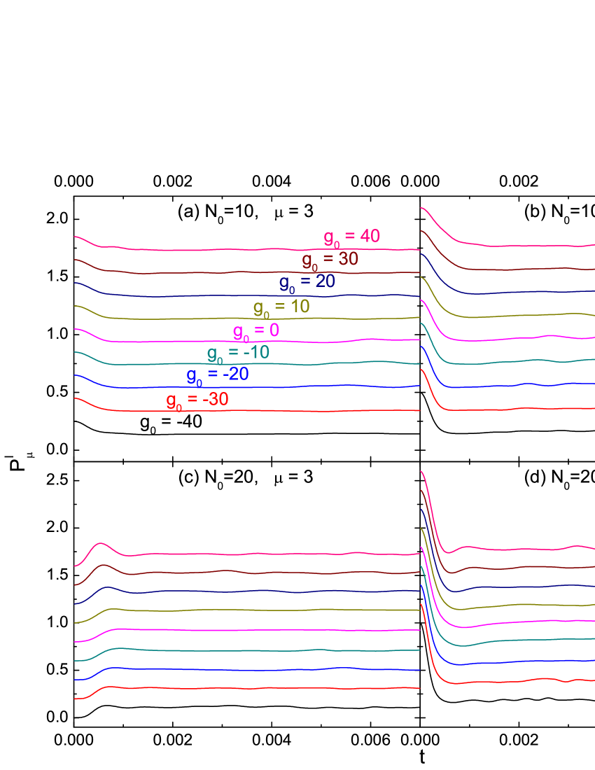
Figure 3: (Color online.) The same as Fig. 2 expect that $N_{0}^{I}=10$ for (a) $\mu=3$ and (b) $\mu=0$, and $N_{0}^{I}=20$ for (c) $\mu=3$ and (d) $\mu=0$, respectively.

IV Conclusion

We study the spin evolution starting from a mixture of two groups of ⁵²Cr atoms, which are fully polarized but in reverse directions and contains only a few particles. And we find an effective way for determining the strength $g_{0}$. In this way, the deviations caused by the SMA and by the neglect of the dipole force are reduced. Accordingly, the theoretical approach becomes much simpler and a calculation beyond the mean field theory is performed. The numerical results show that the knowledge on $g_{0}$ can be thereby extracted. Nonetheless, the above theoretical calculation can only provide a rough evaluation of $g_{0}$. For an accurate determination, more precise theory beyond the SMA and with the dipole force taking into account is necessary. This will lead to a great complexity, and hopefully can be realized in the near future.

- (1) T. L. Ho, Phys. Rev. Lett. 81, 742 (1998)
- (2) T. Ohmi and K. Machida, J. Phys. Soc. Jpn. 67, 1822 (1998)
- (3) D. M. Stamper-Kurn, M. R. Andrews, A. P. Chikkatur, S. Inouye, H.-J. Miesner, J. Stenger, and W. Ketterle, Phys. Rev. Lett., 80, 2027 (1998)
- (4) J. Stenger, S. Inouye, D. M. Stamper-Kurn, H.-J. Miesner, A. P. Chikkatur, and W. Ketterle, Nature (London), 396, 345 (1998)
- (5) C. K. Law, H. Pu, and N. P. Bigelow, Phys. Rev. Lett. 81, 5257 (1998)
- (6) A. Görlitz, T. L. Gustavson, A. E. Leanhardt, R. Löw, A. P. Chikkatur, S. Gupta, S. Inouye, D. E. Pritchard, and W. Ketterle, Phys. Rev. Lett., 90, 090401 (2003)
- (7) M. Lewenstein, A. Sanpera, V. Ahufinger, B. Damski, A. Sen De, and U. Sen, Adv. Phys. 56, 243 (2007)
- (8) A. Griesmaier, J. Werner, S. Hensler, J. Stuhler, and T. Pfau, Phys. Rev. Lett. 94, 160401 (2005)
- (9) R. B. Diener and T.-L. Ho, Phys. Rev. Lett. 96, 190405 (2006)
- (10) J. Stuhler, A. Griesmaier, T. Koch, M. Fattori, T. Pfau, S. Giovanazzi, P. Pedri, and L. Santos, Phys. Rev. Lett. 95, 150406 (2005)
- (11) H. Schmaljohann, M. Erhard, J. Kronjäger, K. Sengstock, and K. Bongs, Appl. Phys. B: Lasers Opt. 79, 1001 (2004)
- (12) M.-S. Chang, C. D. Hamley, M. D. Barrett, J. A. Sauer, K. M. Fortier, W. Zhang, L. You, and M. S. Chapman, Phys. Rev. Lett., 92, 140403 (2004)
- (13) M. S. Chang, Q. Qin, W. Zhang, L. You, and M. S. Chapman, Nature Physics (London) 1, 111 (2005)
- (14) H. Pu, C. K. Law, S. Raghavan, J. H. Eberly, and N. P. Bigelow, Rhys. Rev. A., 60, 1463 (1999)
- (15) R. B. Diener and T.-L. Ho, arXiv:cond-mat/0608732v1 [cond-mat.other] (2006)
- (16) M. Luo, C. G. Bao, and Z. B. Li, Phys. Rev. A 77, 043625 (2008)
- (17) Z. F. Chen, C. G. Bao, and Z. B. Li, arXiv:0802.0822v1 [cond-mat.other] (2008)
- (18) S. Yi, Ö. E. Müstecaplioǧlu, C. P. Sun, and L. You, Phys. Rev. A 66, 011601(R) (2002)
- (19) C. G. Bao, Acta Sci. Nat. Univ. Sunyatseni 46, 70 (2004)
- (20) J. Werner, A. Griesmaier, S. Hensler, J. Stuhler, T. Pfau, A. Simoni, and E. Tiesinga, Phys. Rev. Lett. 94, 183201 (2005)
- (21) Z. B. Li, C. G. Bao, and J. Katriel, Phys. Rev. A 77, 023614 (2008)
- (22) C. G. Bao, Few-Body Syst 46, 87 (2009)