Implications of Dispersal and Life History Strategies for the Persistence of Linyphiid Spider Populations

Abstract

Linyphiid spiders have evolved the ability to disperse long distances by a process known as ballooning. It has been hypothesized that ballooning may allow populations to persist in the highly disturbed agricultural areas that the spiders prefer. In this study, I develop a stochastic population model to explore how the propensity for this type of long distance dispersal influences long term population persistence in a heterogeneous landscape where catastrophic mortality events are common. Analysis of this model indicates that although some dispersal does indeed decrease the probability of extinction of the population, the frequency of dispersal is only important in certain extremes. Instead, both the mean population birth and death rates, and the landscape composition, are much more important in determining the probability of extinction than the dispersal process. Thus, in order to develop effective conservation strategies for these spiders, better understanding of life history processes should be prioritized over an understanding of dispersal strategies.

1 Introduction

Dispersal strategies occur over both short and long spacial scales. At all scales, it has been suggested that dispersal is a bet-hedging or risk-spreading strategy used by organisms to deal with heterogeneous, stochastic environments (Courtney, 1986; Hopper, 1999; Kisdi, 2002). However, dispersal and movement by individuals also have more concrete consequences for populations. It allows them to utilize new resources and areas, it connects separate populations within a metapopulation, and it may help maintain population and metapopulation stability and decrease extinction risk (Hanski, 2001; Hansson, 1991). Dispersal into novel environments can also result in local adaptations and speciation (Clobert, 2001).

Linyphiid, or money, spiders are one example of an animal that employs both short and long distance dispersal strategies (Thomas et al., 1990). For money spiders, long distance dispersal occurs as a mostly passive process known as ballooning (Duffy, 1998). During ballooning, the spider is able to float within air currents, suspended by a single strand of silk. Nearly all Linyphiid species have been observed ballooning, although ballooning propensity varies between species (Thomas et al., 1990; Duffy, 1998). Although it is unknown how far a spider can travel by this method, observations of spiders ballooning over the ocean, far from land (Darwin, 1906), place some bounds on what is possible.

Linyphiid spiders prefer to live in agricultural areas, such as field or pasture land, where they predominantly feed on aphids, although some species are generalist predators (Sunderland et al., 1986). Since they are able to balloon into areas that have been disturbed by agricultural processes, it has also been suggested that Linyphiid spiders may be important for controlling outbreaks of pests in these areas (Sunderland et al., 1986; Thorbek and Topping, 2005). However, the spiders are themselves sensitive to agricultural activities, such as harvesting or pesticide applications (Thomas and Jepson, 1997). Additionally, since the early 1970s, observations indicate that populations of many Linyphiid species have been decreasing, possibly due to climate change (Thomas et al., 2006). Since this decline seems to correlate most strongly with a reduction in days where the weather is appropriate for ballooning, the difference in population outcomes between species may be related to differing dispersal propensities (Thomas et al., 2006). More specifically, particular dispersal strategies may allow some species to better cope with the agricultural landscape, which is characterized by a heterogeneous environment and fairly frequent high-mortality “catastrophes”. However, it is difficult to observe the details of both dispersal and life histories of the spiders directly, so another approach is needed.

Various models of spider ballooning have been developed. Humphrey (1987) first developed a simple one dimensional fluid dynamics model of a single spider, and more recently Reynolds et al. (2006) proposed a stochastic model of the process in a turbulent flow. Thomas et al. (2003) proposed a statistical model for the distances travelled by money spiders in different weather conditions parameterized with data from observations of spiders collected during ballooning. This model indicates that these spiders may be able to travel more than 30 km within a single day (Johnson et al., 2007), which is within observed bounds. However, none of these models address the population consequences for this kind of very long distance dispersal.

There have been previous models that have been constructed to address how dispersal strategies interact with life history strategies and field disturbances to influence Linyphiid population levels. Thorbek and Topping (2005) developed a very detailed Individual Based Model (IBM) for one Linyphiid species, Erigone atra, within a two dimensional landscape. Their model includes details of landscape dynamics (including crop growth and weather, as well as different types of disturbance), stage structured life histories, and environmentally cued dispersal. They primarily focus on how variation in specific landscape activities (such as crop rotation) and landscape compositions effect population sizes. However, the detail and specificity of this model has drawbacks. Many of the conclusions may not be generalizable to other species, and the shear complexity and computational power needed for this type of model can make exploration of the possible behaviors of this system much more difficult. Halley et al. (1996) developed a simpler one dimensional, deterministic model of a spider population composed of “dispersers” and “non-dispersers” in an agricultural landscape. However, like the Thorbek and Topping (2005) model, the specificity of this model, particularly the use of very specific deterministic disturbances, makes it difficult to draw general conclusions about how metapopulation persistence is impacted by factors such as dispersal and life history strategies.

In this paper I examine a simple stochastic model of a metapopulation of ballooning spiders within a heterogeneous environment. The primary goal of the study is to understand how dispersal strategies impact long term population persistence in the face of high levels of habitat disturbance and mortality. I approach the problem in the spirit of a population viability analysis (Boyce, 1992; Coulson et al., 2001; Reed et al., 2002), determining how populations characterized by different life history parameters and dispersal propensities may be more or less likely to go extinct within 110 years when faced with varying levels of catastrophic events. This time horizon is used as it would be a reasonable time frame for conservation targets. I begin by introducing the model in Section 2, followed in Section 3 by the simulation methods used to explore the model. In Section 4, I introduce classification and regression trees (CART), which are used to analyze the simulation output. Results for a baseline case and three variations are presented in Section 5. Section 6 concludes the paper with a short discussion.

2 Model Description

The model presented here is comprised of three portions: a population model with demographic stochasticity within an agricultural field; a data driven dispersal model; and a stochastic environment, incorporating field level catastrophes. The model is formulated as a quasi Individual Based Model (IBM). Whereas a full IBM would follow each particular individual over their whole lifetime, here I employ a novel approach whereby individuals are only followed during the dispersal process – population dynamics and catastrophes are not individual-based. This approach has computational benefits, especially when large numbers of individuals are being modeled.

The landscape considered in this model is comprised of a one dimensional ribbon consisting of patches or fields, each of size $s$, with periodic boundary conditions. Each simulated landscape consists of 50 virtual fields, numbered sequentially from 1 to 50. All fields are the same fixed size, $s=1.3$km, and have the same fixed carrying capacity $K=300$ (i.e., I assume that carrying capacity is constrained by space availability within a field (Halley et al., 1996)).

In discrete time the number of individuals in the $i^{\mathrm{th}}$ patch changes as

$$N_{i}(t+1)=N_{i}(t)-D_{i}+B_{i}-E_{i}+I_{i}$$ (1)

where $D$ are the number of deaths in the patch, $B$ the number of births, $E$ the number of emigrants leaving the patch, and $I$ the number of spiders successfully immigrating to the patch. Figure 1 shows a diagram of the model flow at each time step, which is explained in more detail below.

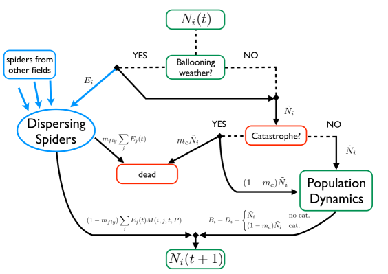
Figure 1: Diagram of Model Flow

Each patch or field is one of $n$ types. Field types are characterized by their “quality”, i.e., by the population birth and death rates within the field. More specifically, spiders in high quality fields could reproduce more quickly or are less likely to die from intrinsic mortality than those in poor quality fields. Births and deaths are modeled using simple stochastic logistic growth such that density dependence acts to regulate reproduction and recruitment into the adult population. In this case, at each time step a spider in field $i$, of type $n$, dies with a probability $b_{n}$ and produces a single (adult) offspring with probability $a_{n}\left(1-\frac{N_{i}}{\kappa_{n}}\right)$ where $\kappa$ is related to the traditional carrying capacity $K$ by $\kappa_{n}=a_{n}K_{n}/(a_{n}-b_{n})$. In other words, I assume that only reproductive rates (and not death rates) are density dependent. Thus the expected number of births (here, recruited adults) and deaths in a single field are given, respectively, by

$$<B_{i}> =a_{n}(\tilde{N}_{i})\left(1-\frac{\tilde{N}_{i}}{\kappa_{i}}\right)$$ (2)

$$<D_{i}> =b_{n}\tilde{N}_{i}$$ (3)

where $\tilde{N}_{i}=N_{i}-E_{i}$ are the number of spiders that do not disperse at time $t$.

Two hypotheses of dispersal are considered in the model: density independent and density dependent. Thus the number of spiders emigrating or dispersing from the $i^{\mathrm{th}}$ field at time $t+1$ can either be a fixed proportion of the population in the patch at time $t$,

$$<E_{i}>\;=p_{\mathrm{disp}}N_{i}(t),$$ (4)

or can vary with population density as

$$<E_{i}>\;=p_{\mathrm{disp}}\frac{N_{i}^{2}(t)}{K_{i}},$$ (5)

where $K_{i}$ is the carrying capacity in the $i^{\mathrm{th}}$ field, and where we constrain $<E_{i}>\;\leq N_{i}(t)$. Thus, as $N_{i}(t)\rightarrow K_{i}$ the proportion of individuals dispersing is the same for both the density dependent and density independent cases. When $N_{i}<K_{i}$ spiders are less likely to disperse when there is density dependent dispersal than density independent dispersal, and vice versa for the case when $N_{i}>K_{i}$. During dispersal, emigrants avoid mortality in the patch but die with probability $m_{\mathrm{fly}}$. The mortality during dispersal could include multiple factors such as predation or desiccation. However, for simplicity here I assume a constant daily mortality rate while dispersing. Spiders also cannot reproduce as they disperse.

The number of spiders that immigrate into the $i^{\mathrm{th}}$ patch is given by the sum of the spiders that leave all the fields ($E_{j}$), survive dispersal, and consequently arrive in the $i^{\mathrm{th}}$ field. The dispersal kernel $M(i,j,t,P)$ describes the probability that a spider starting in field $j$ lands in field $i$ on day $t$ given parameters, $P$. The data-driven model used to generate the dispersal dynamics is presented in Section 2.1.

Spiders will only attempt to disperse under favorable weather conditions. I assume that daily conditions are good for dispersal with some fixed probability, $p_{\mathrm{fly}}$. In other words, out of $\mathcal{D}$ days, the number of days with conditions favorable for dispersal, $d$, is binomial with success probability $p_{\mathrm{fly}}$: $d\sim\mathrm{Binomial}(\mathcal{D},p_{\mathrm{fly}})$. Whenever conditions are favorable the numbers of spiders that attempt to disperse are given by Equation (4) or (5), and when conditions are not favorable $E_{i}=0$ in every field.

In the fields, “catastrophes”, i.e., mortality events that wipe out significant proportions of spiders in a particular field, can occur (Thomas and Jepson, 1997). A catastrophe with mortality rate $m_{c}$ occurs on a given day with probability $p_{c}$. Catastrophes occur after dispersal has begun (so that dispersing spiders can escape catastrophes) but before births or (intrinsic) deaths. In addition, all parameters that determine dispersal behaviors or population dynamics are fixed and constant through time.

I am primarily interested in how variation of four parameters, given the other parameters as fixed (see Table 1 and Section 2.1), influences the probability of extinction. Specifically I look at: the probability of catastrophe, $p_{c}$; the probability of weather suitable for flying, $p_{\mathrm{fly}}$; the probability that a spider disperses in good weather, $p_{\mathrm{disp}}$; and the mortality rate experienced during flying, $m_{\mathrm{fly}}$. In addition, the dispersal probability can be either density dependent or density independent. The catastrophe rate, $p_{c}$, is regarded here as being primarily human induced mortality, for example due to application of pesticides in a field. Two of the parameters, $p_{\mathrm{fly}}$ and $m_{\mathrm{fly}}$, can be viewed as environmentally determined parameters. The parameter $p_{\mathrm{fly}}$, which may be decreasing for these spiders due to climate change (Thomas et al., 2006), constrains the opportunities for dispersal into new habitats, and the ability for spiders employing any dispersal strategy to escape local mortality events. The mortality rate during dispersal, $m_{\mathrm{fly}}$, includes mortality from various factors, such as predation and desiccation. Thus the spiders must weigh the risks of dispersing against the risks of catastrophes or benefits of reproduction if remaining in a field. The final parameter, $p_{\mathrm{disp}}$, together with the options for density dependence or not, thus determine what I consider the evolved “dispersal strategy”.

Symbol	Description	Value or Range
$k$	number of fields/patches	50
$s$	field size (km)	1.3
$n$	number of types of fields	5
$K$	field carrying capacity (spiders)	300
$m$	dispersal time in each day (minutes)	$(0,480)$
$m_{c}$	mortality level in a catastrophe	95 %
$b_{i}$	per capita death rate in the $i^{\mathrm{th}}$ field	0.02
$a_{i}$	per capita birth rate in the $i^{\mathrm{th}}$ field	[0.05, 0.2875, 0.525, 0.7625, 1]
$p_{\mathrm{fly}}$	daily probability of suitable dispersal weather	$(0,1)$
$m_{\mathrm{fly}}$	daily mortality rate in flight	$(0,1)$
$p_{\mathrm{disp}}$	probability a spider disperses, given good weather	$(0,1)$
$p_{c}$	daily probability of catastrophe, per field	$(0,0.5)$
($v_{1}$,$g$)	wind speed at 1m, wind speed gradient	$(2.2,1.25)$
$E$	ascent/descent parameter	2.5
$1/\lambda$	mean waiting time (minutes)	12

Table 1: Parameters and their values or ranges in for the baseline simulations

2.1 The Dispersal Model

I utilize an established statistical model for the ballooning dispersal kernel, parameterized with observational data (Thomas et al., 2003; Johnson et al., 2007). For this approach, dispersal is modeled as follows (see Figure 2). Suppose that on a day with appropriate weather for ballooning, there are $m$ minutes of good weather for dispersal (specifically, take-off). At the beginning of the day, each spider decides to begin dispersal attempts with probability $p_{\mathrm{disp}}$. Upon attempting to disperse, the spider first waits some time $\tau$ before successfully ballooning. The waiting time has a exponential distribution so that $\tau\sim\mathrm{Exp}(\lambda)$, where the mean waiting time (12 minutes, corresponding to $\lambda=\frac{1}{12}$) is fitted from observational data. When the spider successfully takes off, it will travel some distance $d$ during its flight. The distance is calculated from the maximum height, $h$, that the spider can achieve in a flight, with the distribution of heights given by

$$f(h)=c_{1}b(h^{-b}-h^{-(b+1)})$$ (6)

for $1<h<h_{\mathrm{max}}$, where $h_{\mathrm{max}}$ is the maximum possible height (here 1000m), $b$ describes changes of spider density with height (from field data), and $c_{1}$ is a normalization constant. Flights consist of an ascent at a fixed rate $\alpha$ up to the maximum height, then a descent at rate $\delta$, the terminal velocity. The horizontal wind speed varies with height and is parameterized using field data. Single flight distances $l$ are calculated by integrating wind speed for heights up to $h$,

$$l=\begin{cases}\frac{1}{E}\left(hv_{1}+\frac{(h+1)\ln(h+1)-h}{g}\right)&h\leq 100\\ \frac{1}{E}\left(100v_{1}+\frac{(101)\ln(101)-100}{g}\right)+\left(\frac{h-100}{E}\right)\left(\frac{\ln(101)}{g}+v_{1}\right)&100<h<1000,\end{cases}$$ (7)

where $E$ is the ascent/descent parameter, defined as $1/E=1/\alpha+1/\delta$, and $v_{1}$ and $g$ are the wind speed at 1m and the wind speed gradient, respectively. Both of these parameters are estimated from observational data (Thomas et al., 2003).

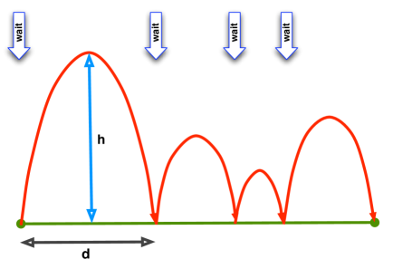
Figure 2: Schematic representation of the dispersal process.

During a day with $m$ minutes of good weather for dispersal, the spider alternates waiting and flying (see Figure 2). The spider continues attempting to take-off throughout the entire time available for flying, in order to travel the furthest distance possible. At the end of the day, it has travelled a total distance $L$, and will generally be in a new field. Figure 3 shows simulated travel distances from this dispersal model for the flight parameters used in the simulations. Note that in these conditions very large dispersal distances are possible – up to 30 km when there are 8 hours of appropriate weather. However, even with only half an hour of good weather dispersal distances of 5-7 km are possible. This implies that spiders are very likely to reach another field, since fields in agricultural landscapes are generally less than 5 km in length (Halley et al., 1996), and on especially fine days spiders dispersing from a single field are likely to end up spread across a very wide area.

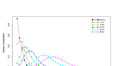
Figure 3: Simulated distributions of total flight distances achieved by spiders during dispersal episodes of $m=\{0.5,1,2,3,6,8\}$ hours with wind speed parameters $v_{1}=2.2$ and $g=0.8$, and ascent/descent parameter $E=2.5$.

We could approximate the dispersal kernel, $M(i,j,t,P)$, with $P=\{h_{a},h_{b},E,m,\lambda\}$, described by this model via Monte Carlo simulation of individual flights interspersed with waiting. In many cases the number of simulations needed to approximate this kernel is greater than the total numbers of individuals dispersing at any given time in the simulation. Thus I instead directly simulate the path of each dispersing spider individually to place them in a new field at the end of the dispersal step.

3 Model Parameterization and Simulations

For a model such as the one presented here the probability of extinction within some fixed period of time cannot be found analytically. Instead a simulation approach must be used. More specifically, simulations are performed to find the probability that the meta-population, under specific dynamics and environmental conditions described by a set of parameters, will go extinct within 110 years.

Simulation parameters and their values are summarized in Table 1. Birth and death rates are not well known for most Linyphiid species. For the baseline case I assume a daily intrinsic mortality rate of $b_{i}=0.02$, which gives a mean lifespan of 50 days. This is lower than has been observed in controlled laboratory settings, where spiders can live for more than 100 days, but seems reasonable as first approximation to natural populations . In laboratory experiments egg production levels and the proportion of eggs produced which are viable are quite variable across food regimes and species . Thus the range of parameters assumed for the per capita “birth” rates in the fields, $a_{i}$, (here, rates or recruitment to adult class) are broad (see Table 1). At the extremes of this range, the expected number of adult offspring produced by a single spider that lives for 50 days in a single field ranges from 2.5 to 50. Thus the five field types correspond to the five levels of $a_{i}$ specified in Table 1, since $b_{i}$ is fixed.

The set of parameters that determine the dispersal kernel are fitted from observations of spiders on a single day, and are given in Table 1. Weather appropriate for ballooning tends to occur mostly in the morning through to early afternoon (Thomas et al., 2003). Thus I assume that the amount of time during the day that is suitable for the initiation of dispersal, $m$, is uniformly distributed from zero up to 8 hours.

Observed mortality levels for spiders during disturbances can vary fairly widely. For instance, mortality levels of around 20% from residual toxicity from pesticide application (Thomas, 1992), or 56% to $>95$% during the application of insecticides or other agricultural operations have been observed (Thomas and Jepson, 1997). For the simulations presented here, I assume that the morality level during a catastrophe is constant between fields and over time, and is set to the high end of the observed range (95%) as a worst-case scenario.

Each simulation experiment consists of both density dependent and density independent dispersal cases. For each of these two cases, 500 parameter combinations of the four parameters of interest ($p_{c}$, $p_{\mathrm{disp}}$, $p_{\mathrm{fly}}$, $m_{\mathrm{fly}}$) were chosen as a Latin-hypercube sample (LHS) (McKay et al., 1979) to efficiently explore the response within the parameter space. Thus, one complete simulation experiment consists of 1000 parameter/density combinations. In each simulation, the landscape composition (i.e., the assigned “type” of each field in the ribbon) is randomly chosen from an appropriate distribution. Initially, populations in all fields are set to the carrying capacity. The simulation output consists of binomial extinction/survival results, as well full population trajectories for a random subset of the simulations.

Each simulation in the experiment is run for 400,000 virtual days ($\approx 110$ years) or extinction ($\sum_{i}N_{i}(t)\leq 1$), whichever is first. For each parameter set, at least 2 runs are performed with 10% of the parameters randomly chosen for a third run, for a total of approximately 2100 simulations. The experiment is repeated for four cases, each of which I describe below.

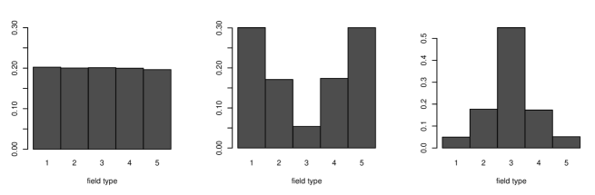
(a)

(b)

(c)

Figure 4: Draws from the multinomial distributions used to determine the field compositions in (a) the baseline main simulation discussed Section 3.1 and (b) & (c) the two variations discussed in Section 5.2

3.1 Baseline Simulations

The first of the simulation experiments is the “baseline” case. The field parameters used for this set of simulations are given in Table 1. The landscape composition is determined by choosing fields uniformly (Figure 4(a)) from the 5 possible field “types”, corresponding to the the 5 possible values of the per capita birth rate, $a_{i}$, given in Table 1.

3.2 Baseline with High Variance in Field Composition (Best/Worst)

In the second simulation experiment, I begin to explore the effects of changing the distribution of field types (relative proportions of high vs. low quality fields) in the landscape while leaving the types of fields (the birth and death rates) the same as in the baseline case. Whereas in the baseline case 3.1 the distribution of fields was uniform (Figure 4(a)), in the second experiment I consider the case where most fields are either very good or very bad, with fewer of intermediate quality, as shown in Figure 4(b). This results in the same mean birthrate throughout the fields, $\bar{a}=0.50$ as in the baseline case. However, here the variance is higher, $\mathrm{Var}(a)\approx 0.156$. Throughout the rest of the paper I will refer to this case as the “Best/Worst” scenario.

3.3 Baseline with Low Variance in Field Composition (Many Moderate)

In the third simulation experiment, I again explore the effects of changing the distribution of field types. However, in this case the trend is the opposite of the Best/Worse scenario: there are many moderately good fields, and fewer of both the low and high quality fields (Figure 4(c)). Again this distribution has the same mean birthrate throughout the fields, but has lower variance than either of the previous two experiments, $\mathrm{Var}(a)\approx 0.0425$. In the discussion that follows, I refer to this experiment as the “Many Moderate” scenario.

3.4 Variation in Birth and Death Rates (Population II)

The three scenarios that I have described thus far all assumed the same set of birth and death parameters in the fields, and only varied the relative proportion of each. In the final experiment, I assume a new set of birth and death rates. This could correspond to the same species within a significantly different landscape, or a different species within the previous landscape. Specifically, the within field mortality level is increased compared to the baseline so that $b=0.05$, and let the per capita birthrate in the $i^{\mathrm{th}}$ field is drawn from the set $a_{i}=[0.06,0.1,0.25,0.3,0.79]$ That is, this population experiences two types of “very low” quality fields, two “low” types, and one “very good”. The distribution of these fields within the landscape is uniform, i.e., the field type is drawn from the multinomial distribution shown in Figure 4(a). This set of birthrates has mean $\bar{a}=0.3$, which is lower than the baseline case, and variance $\mathrm{Var}(a)\approx 0.07$, which is intermediate compared to cases already explored. In the analysis below I will refer to this experiment as “Population II”.

4 Data analysis with CART

The simulation output (survival or extinction) can be treated as binary data, and could be modeled in a number of ways. One traditional statistical approach would be to look for the dependence of the probability of extinction upon the parameters determining environmental condition and dispersal strategy using a regression approach, such as a generalized linear model (GLM) (McCullagh and Nelder, 1990). However, this approach is not appropriate for these data, as the typical checks of the assumptions of additive and homoskedastic error are not satisfied (data not shown). Instead, I take a classification and regression tree (CART) approach (Breiman et al., 1984), which is a non-parametric statistical model that allows for heteroskedastic errors and is applicable to both numerical and categorical data.

In a GLM-type analysis we would appeal to the likelihood ratio test to test for the significance of parameters, and proceed iteratively via the forward/backward method to settle upon a final model. Building trees proceeds in a similar, but usually non-iterative, manner. First the Gini impurity (Breiman et al., 1984) maybe used to go forward and “grow” the tree (add splits/branches). Then cross-validation (CV) is used to “prune” the tree back (remove splits/branches). All trees in the following sections were fit using the rpart package (Therneau and port by Brian Ripley., 2008) in R (R Development Core Team, 2008). In the rpart package, the degree of pruning is determined by a complexity parameter ($C_{p}$) (Mallows, 1973) that may be chosen by the one-standard-error rule (Hastie et al., 2001, Section 7.10), or other similar methods. For more details on fitting treed models in R or S see Venables and Ripley (1999).

One advantage of a CART-type model is that the interpretation of (pruned) tree diagrams is fairly straightforward. The goal of the diagram is to indicate for what values of various predictor variables the model predicts a given probability of a response variable. In the case explored here, the real-valued predictors are: $m_{\mathrm{fly}}$; $p_{c}$; $p_{\mathrm{fly}}$; $p_{\mathrm{disp}}$; and we have a binary class-type predictor {dense, not dense}. The response variable is extinction in 110 years. Since the tree is built interactively by finding the variable at each split that best explains the variation in the response, earlier splits are generally the most important for understanding the response. If a tree does not split on a particular variable, and the variable is not correlated with the variables that do appear, then knowing the value of the variable does not significantly improve one’s knowledge of the probability of observing the response variable.

At each node in the tree, a Boolean expression is given, together with some indication of a value or range of values for that parameter. For instance in Figure 6, the first node is labeled as $p_{c}<0.223$. The nodes dangling from the branches here are called the children, or child nodes. The child nodes dangling from the left branch of this top node operate on data satisfying this Boolean expression; the child nodes dangling from the right branch violate it. Thus in Figure 6 the left half of the tree corresponds to the cases where $p_{c}<0.223$ and the right half of the tree corresponds to $p_{c}\geq 0.223$. Branches can spilt at the children (for instance in Figure 6, the left child has another spilt at $m_{\mathrm{fly}}<0.6712$), until the branches terminate at “leaves”. Each leaf in the tree diagram here is labeled with the probability that the response variable (extinction) is true, and the number of observations/simulations which lie in the portion of the parameter space described by the branches leading to the leaf. Thus, the values at the left-most leaf in Figure 6 indicate that the probability of the population going extinct within 110 years, if $p_{c}<0.223$ and $m_{\mathrm{fly}}<0.6712$, is $<3$%, based on 290 simulations.

5 Results

Figure 5 gives examples of simulated population trajectories for a portion of the landscape (20 out of 50 fields) during the first 700 days. Results ranged from populations going extinct (or very nearly) early on (Figure 5a) to very large populations across many of the fields (Figure 5b). In simulations where populations were large and persistent, variation in field populations was due to differences in the habitat parameters in the different fields. Patterns tended to stabilize quickly, and most populations either went extinct very rapidly ($<100$ days, for example in Figure 5 (a), top), or persisted for the maximum duration explored here. In the remaining analysis I focus on the extinction/survival output.

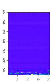
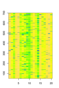
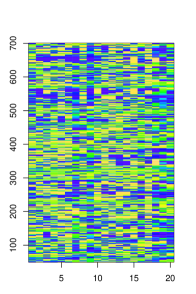
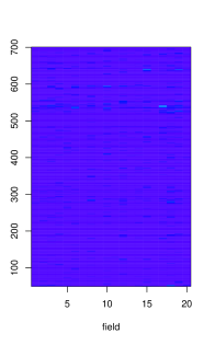
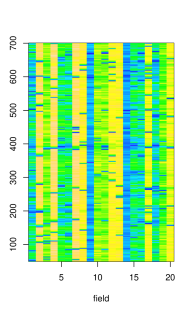
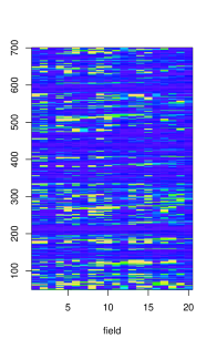
(a)	(b)	(c)

Figure 5: Examples of density dependent (top) vs density independent (bottom) dispersal for three parameter settings with random field configurations. Fields are arranged in a line and are labeled by a location x-axis, and time on the y-axis. Violet indicates low or zero population size in a field and yellows larger populations.

5.1 Baseline Scenario

I begin with the baseline case, as described in Section 3.1. The pruned tree for the full data set is shown in Figure 6. Even with the appropriate pruning the tree is fairly complicated. First, we notice that the probability of catastrophe, $p_{c}$, is the most important determinant of extinction probability, as the initial branching depends on $p_{c}$, and there are more branchings in the tree that depend on $p_{c}$ than any other factor. The tree can be approximately viewed as having three regions with low ($p_{c}<0.22$), medium ($0.22<p_{c}<0.31$), and high ($p_{c}>0.31$) probability of catastrophe, that loosely correspond to low, medium, and high probability of extinction within 110 years.

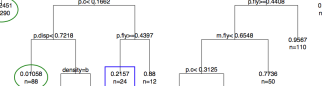
Figure 6: Pruned tree showing the parameters and values that most determine the probability of metapopulation extinction within 100 years for baseline scenario (Section 3.1). The splits from each node follow the rule left=TRUE. Density values of $\{a,b\}$ indicate density independent and dependent dispersal, respectively. Leaves with extinction probability of $<0.1$ are indicated with circles, and those with $<0.4$ with squares.

For most of the parameter space, the particular dispersal strategy employed, (i.e., the probability of dispersing given good weather, $p_{\mathrm{disp}}$, and density dependent or independent dispersal) is not particularly important. When the risk of catastrophe is low, as long as the inflight mortality is low enough ($m_{\mathrm{fly}}<0.67$), populations employing any dispersal strategy are predicted to have a low probability of extinction. However, when in-flight mortality is higher than this, populations are only likely to persist when catastrophe levels are are low ($p_{c}<0.1662$) and, simultaneously, either dispersal propensity is not too high ($p_{\mathrm{disp}}<0.72$) or density dependent dispersal is used (which reduces the effective dispersal propensity as long as the population is below the carrying capacity). In other words, when dispersal mortality is very high, frequent dispersal increases the probability of population extinction, as one might expect.

At intermediate catastrophe levels (here $0.223<p_{c}<0.31$) populations only persist in a very narrow range of circumstances where the probability that a day has good weather for dispersal is greater than 44% (more than 160 days per year) and, simultaneously, the inflight mortality rate is not too high ($m_{\mathrm{fly}}<0.65$). In other words, for the population to persist under intermediate disturbance, there need to be adequate opportunities for at least some of the spiders to disperse and survive to reach a new field. Outside of this area of the parameter space, the probability of a population persisting, particularly for catastrophe levels of over $0.3$, is very low ($\approx$ 5-20%) .

5.2 Best/Worst and Many Moderate Scenarios

Figure 7 shows the results for the Best/Worst scenario, which is characterized by high variance in the birthrates. First we notice that, as in Section 5.1, the strategy employed by the spiders is not particularly important for determining the extinction probability (i.e., the tree only has a few splits, near the leaves, that depend on either $p_{\mathrm{disp}}$ or “dense”). Again the most important consideration is the level of catastrophe. However, notice that in this case the population is actually less sensitive to low levels of disturbance, where the population has a very good chance of persisting (extinction probabilities of $\approx 0.009$ to 0.1), as long as $p_{c}<0.21$. This is likely due to the increased abundance of high quality fields. Like the baseline case, the exception to this is when both in-flight mortality and dispersal propensity are high ($m_{\mathrm{fly}}>0.67$ and $p_{\mathrm{disp}}>0.72$, respectively) and individuals utilize density independent dispersal. In this case, populations have a greater than 70% chance of going extinct.

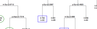
Figure 7: Pruned tree showing the parameters and values that most determine the probability of metapopulation extinction within 100 years for ”Best/Worst” scenario. (See Section 3.2) The splits from each node follow the rule left=TRUE. Density values of $\{a,b\}$ indicate density independent and dependent dispersal, respectively. Leaves with extinction probability of $<0.1$ are indicated with circles, and those with $<0.4$ with squares.

Figure 8 shows the results for the Many Moderate scenario, characterized by lower variance in the birthrate. The resulting tree is nearly identical to the Best/Worst scenario. However, in this scenario, populations are slightly more likely to go extinct (extinction probability of $\approx 0.02$) when both the probability of catastrophes and inflight mortality rates are low ($p_{c}<0.211$, $m_{\mathrm{fly}}<0.7$) compared to the Best/Worst case; instead the extinction probabilities more similar to the Baseline.

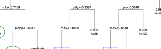
Figure 8: Pruned tree showing the parameters and values that most determine the probability of metapopulation extinction within 100 years for the ”Many Moderate” scenario. (See Section 3.3) The splits from each node follow the rule left=TRUE. Density values of $\{a,b\}$ indicate density independent and dependent dispersal, respectively. Leaves with extinction probability of $<0.1$ are indicated with circles, and those with $<0.4$ with squares.

5.3 Population II scenario

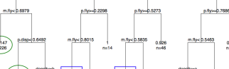
Figure 9: Pruned tree showing the parameters and values that most determine the probability of metapopulation extinction within 100 years for the Population II scenario, characterized by birthrate parameters $a=\{0.79,0.3,0.25,0.1,0.06\}$ (mean birthrate of $\bar{a}=0.3$, or 57% of the baseline mean) and death rate parameter $b=0.05$ (death rate 2.5 times higher than the baseline) and with a uniform distribution of field types as shown in Figure 4 (a). This . (See Section 3.4) The splits from each node follow the rule left=TRUE. Density values of $\{a,b\}$ indicate density independent and dependent dispersal, respectively. Leaves with extinction probability of $<0.1$ are indicated with circles, and those with $<0.4$ with squares.

Figure 9 shows the results for the final scenario explored in this paper, the population II case. As one would expect, since the intrinsic death rate is higher than the previous cases and the mean birth rate is lower, much more of the parameter space results in the extinction of the population. The threshold level of catastrophe that results in a low probability of extinction is $p_{c}\approx 0.17$, which is quite a bit lower than any of the previous cases. Even with this low level of catastrophe, the population is still only likely to persist if the dispersal mortality is low enough ($m_{\mathrm{fly}}<0.7$), the probability of dispersing on a day with good weather is not too high ($p_{\mathrm{disp}}<0.65$), or density dependent dispersal is utilized.

5.4 Results Summary

The results from all of the scenarios explored above show many similarities. For instance, much of the tree structures, such as primary splits depending on $p_{c}$, correlations between $m_{\mathrm{fly}}$ and $p_{\mathrm{disp}}<0.65$, and density dependence only being important in limited circumstances. In each case, the probability of catastrophe determines the probability of extinction within 110 years more than any other factor. The similarities between the left-most branch in all four of the scenarios also indicates that the product of in-flight mortality rate and dispersal propensity, which together determine the expected proportion of individuals within a field that will die on a day with good conditions for dispersal, may be an important threshold for determining extinction probability for a given catastrophe level. However the quantitative results (especially locations of splits) exhibit more variation. In particular, the results indicate that the values of population parameters (birth and death rates) are considerably more important for determining population persistence at a given catastrophe level than the relative abundance of the different types of fields, which in turn has a greater impact than changes in the dispersal strategy (dispersal propensity and density dependence).

6 Discussion

The results of the model presented in this study suggest that, although a general dispersal ability is important for the persistence and growth of Linyphiid spider populations, the exact details of this dispersal strategy, i.e., whether dispersal is density dependent and the particular probability of dispersing on a day with appropriate weather, are less important than other factors in determining persistence in the face of field level catastrophes. Instead, actual catastrophe probability seems to be the most important factor in determining the extinction probability, given landscape and life history parameters. As demonstrated, one may observe thresholds in the catastrophe level where the population switches from being very unlikely to being very likely to go extinct. For instance, results for populations with life histories and landscape distributions described by the parameters in the baseline simulation suggest that if the daily probability of a catastrophe is greater than 22%, then there is greater than 80% chance of extinction within 100 years. Otherwise, there is less than 10% chance that the population would go extinct. The baseline results also make it apparent that reducing the catastrophe level further can help to mitigate the effects of mortality during dispersal.

Although the model presented here fairly simple, it is able to capture patterns that have been observed in more complex models. For instance, the model developed by Halley et al. (1996) exhibited similar thresholding behavior in population size/persistence with catastrophic events, specifically landscape wide pesticide application (all fields affected). They found that if all the fields were of the same type, the population could persist (i.e., the population was $>0$) if the field was sprayed no more than once per year with a pesticide that caused 90% mortality. By including a second field type that is less ideal for habitat, but is not sprayed, the population remains large even with higher frequency of pesticide application in other fields. In the current study we find a similar increase in persistence by limiting the average catastrophe rate across fields, instead of explicitly including refuge habitats. This indicates that for highly dispersive species, undisturbed land for refuges may not be as necessary for population persistence as lower mean disturbance rates, although providing refuges may be an efficient method for reducing the mean disturbance rate. This is a similar result to one reported by Thorbek and Topping (2005) who found that some habitat needed to be available for spiders at all times, although the habitat did not need to be permanent.

On the other hand, by using a more simple model for some aspects, such as the life history, I have been able to focus more on the more general question of the relative importance of dispersal strategy compared to other population and landscape factors for population persistence in the face of catastrophes. Although many of the qualitative results of this model did not depend upon the life history and landscape parameters, the quantitative predictions and, more importantly, the threshold catastrophe levels do depend upon the assumptions about the distribution of field quality in the landscape, reproductive rates, and baseline mortality. On the other hand, the particulars of the dispersal strategy adopted by the spider (such as density dependence or dispersal propensity) were not particularly important under most circumstances. This is in contrast to Halley et al. (1996), who found a fairly strong dependence between population size/extinction and the proportion of individuals dispersing. This difference is could be due to a number of different factors. One possibility is that this the effect of dispersal is less apparent in the current model due to significant stochasticity in all of the model processes. Another is that the difference could be an effect of the stage structured population dynamics, which may result in the particular amount of dispersal being more important in recovery from a catastrophe. A third possibility is related to the fact that the optimal proportion of dispersers in the Halley et al. (1996) study was also strongly related to the proportion of non-habitat patches within the landscape. This factor changes the risk of mortality while dispersing, while simultaneously altering the population reproduction parameters, and seems to be more important in determining the maximum population level than the other factors they explored. A final possibility is that the difference could also be due to the fact that Halley et al. (1996) assume that each individual spider is either a “disperser” or “non-disperser” for its entire life-cycle. This factor may also be part of why Halley et al. (1996), and Thorbek and Topping (2005) draw conflicting conclusions about the effect of field rotations on the population. If a portion of the population are “non-dispersers”, then rotating a field would effectively increase the catastrophe level for a large portion of the population, since these individuals cannot escape a dramatic change in mortality due to the rotation by dispersing. Although I do not deal with rotation explicitly in this model, I expect it would have a similar, though mild, effect here, as long as the rotations do not change the overall distribution of fields in the landscape dramatically.

Since there is such a strong interaction between the effect of population parameters and catastrophe level, the current study suggests that the current patterns of decline are likely to be due to a combination of both changing life histories and agricultural practices (field composition and catastrophe level). In order to preserve or increase spider populations in the future, we may want to suggest conservation measures that seek to curb the levels of human induced catastrophes in the environment. The observed thresholding behavior in the model indicates that the development of a simple guideline may be possible. For the parameters explored here the thresholds were in the 20% range. In other words, $\sim$ 20% of fields experience catastrophic mortality on a given day, and in a single field we expect nearly 10 weeks worth of high mortality days each year. Although pesticides applied to fields can remain toxic to spiders for more than two weeks after application (Halley et al., 1996), and other types of disturbances also cause significant mortality (Thomas and Jepson, 1997), the predicted threshold seems to be fairly high. However, this value depends fairly strongly on model parameters, especially the population birth and death rates. Thus, more observational data on the reproductive capabilities of target species within various types of agricultural fields, and how these may be affected by climate change, would be most useful for estimating this threshold. Data gathered to estimate different dispersal behaviors/propensities or changes in the proportion of days that are suitable for ballooning would be less useful.

In the current simulations, the effect of a reduction in the number of “habitat” fields has not been explored. This is partly because the effect of reducing carrying capacity, $K$, on metapopulations is fairly well understood (Mangel and Tier, 1993a, b). The addition of “non-habitat” fields at random into the landscape, without reducing the total $K$, would be equivalent to raising the level of mortality during dispersal.

The current model focuses on the case where there are no spatiotemporal correlations in either catastrophes or reproductive schedules. It may be that these kinds of correlations could reduce the tolerance of a population to disturbance, or make other dispersal strategies, such as ones signalled by external factors, more important. Including these factors this would be an important aspect of future work.

7 Acknowledgements

L. R. J. was funded by BBSRC grant D20476 as part of the National Centre for Statistical Ecology. Thanks to: George Thomas for unpublished data and biological expertise on Linyphiid life histories; Bobby Gramacy for advice on statistical methods; Ian Carroll for comments on an earlier draft; and two very helpful and thorough reviewers.

References

- Boyce [1992] Mark S. Boyce. Population viability analysis. Annual Review of Ecological Systems, 23:481–506, 1992.
- Breiman et al. [1984] Leo Breiman, Jerome Friedman, Charles J. Stone, and R.A. Olshen. Classification and Regression Trees. The Wadsworth statistics/probability series. Wadsworth International Group, Belmont, CA, 1984.
- Clobert [2001] Jean Clobert, editor. Dispersal. Oxford University Press, Oxford, UK, 2001.
- Coulson et al. [2001] Tim Coulson, Georgina M. Mace, Elodie Hudson, and Hugh Possingham. The use and abuse of population viability analysis. TRENDS in Ecology and Evolution, 16(5):219–221, May 2001.
- Courtney [1986] Steven P. Courtney. Why insects move between host patches: some comments on ‘risk-spreading’. Oikos, 47(1):112–114, July 1986.
- Darwin [1906] Charles Darwin. Journal of reseraches into the natural history and geology of the countries visited during the voyage of HMS Beagle around the world, chapter VIII. Everyman’s Library, Dent, London, 1906.
- Duffy [1998] E. Duffy. Aerial dispersal in spiders. In P.A. Selden, editor, Proceedings of the 17th European Colloquium of Arachnology, pages 189–191, Burnham Beeches, UK, 1998. British Arachnological Society.
- Halley et al. [1996] J. M. Halley, C. F. G. Thomas, and P. C. Jepson. A model for the spatial dynamics of linyphiid spiders in farmland. Journal of Applied Ecology, 33(3):471–492, 1996. URL doi:10.2307/2404978.
- Hanski [2001] Ilkka Hanski. Population dynamic consequences of dispersal in local populations and in metapopulations, chapter 20, pages 283–298. In Clobert [2001], 2001.
- Hansson [1991] Lennart Hansson. Dispersal and connectivity in metapopulations. Biological Journal of the Linnean Society, 42:89–103, 1991.
- Hastie et al. [2001] T. Hastie, R. Tibshirani, and J. Friedman. The Elements of Statistical Learning: Data Mining, Inference, and Prediction. Springer, 2001.
- Hopper [1999] Keith R. Hopper. Risk-Spreading and Bet-Hedging in Insect Population Biology. Annual Review of Entomology, 44:535–560, 1999.
- Humphrey [1987] J. A. C. Humphrey. Fluid mechanic constraints on spider ballooning. Oecologica, 73:469–477, 1987.
- Johnson et al. [2007] L. R. Johnson, C. F. G. Thomas, P. Brain, and P. C. Jepson. Correction to: Aerial activity of linyphiid spiders: modelling dispersal distances from meteorology and behavior. Journal of Applied Ecology, 2007.
- Kisdi [2002] Éva Kisdi. Dispersal: Risk spreading verses local adaptation. The American Naturalist, 159(6):579–596, June 2002.
- Mallows [1973] C. L. Mallows. Some comments on cp. Technometrics, 15:661–675, 1973.
- Mangel and Tier [1993a] Marc Mangel and Charles Tier. Dynamics of metapopulations with demographic stochasticity and environmental catastropes. Theoretical Population Biology, 44(1):1–31, 1993a.
- Mangel and Tier [1993b] Marc Mangel and Charles Tier. A simple direct method for finding persistence times of populations and application to conservation problems. PROC, 90(3):1083–1086, February 1993b.
- McCullagh and Nelder [1990] Peter McCullagh and John A. Nelder. Generalized Linear Models. CRC Press, 2nd edition, 1990.
- McKay et al. [1979] M. D. McKay, W. J. Conover, and R. J. Beckman. Comparison of three methods for selecting values of input variables in the analysis of output from a computer code. Technometrics, 21:239–245, 1979.
- R Development Core Team [2008] R Development Core Team. R: A Language and Environment for Statistical Computing. R Foundation for Statistical Computing, Vienna, Austria, 2008. URL http://www.R-project.org. ISBN 3-900051-07-0.
- Reed et al. [2002] J. Michael Reed, L. Scott Mills, John B. Dunning Jr., Eric S. Menges, Kevin S. McKelvey, Robert Frye, Steven R. Beissinger, Marie-Charlotte Anstett, and Philip Miller. Emerging issues in population viability analysis. Conservation Biology, 16(1):7–19, Februrary 2002.
- Reynolds et al. [2006] A. M. Reynolds, D. A. Bohan, and J. R. Bell. Ballooning dispersal in arthropod taxa with convergent behaviours: dynamic properties of ballooning silk in turbulent flows. Biology Letters, 2(3):371–373, 2006. URL doi:10.1098/rsbl.2006.0486.
- Sunderland et al. [1986] K. D. Sunderland, A. M. Fraser, and A. F. G. Dixon. Field and laboratory studies on money spiders (linyphiidea) as predators of cereal aphids. Journal of Applied Ecology, 23:433–447, 1986.
- Therneau and port by Brian Ripley. [2008] Terry M Therneau and Beth Atkinson. R port by Brian Ripley. rpart: Recursive Partitioning, 2008. URL http://mayoresearch.mayo.edu/mayo/research/biostat/splusfunctions.cfm. R package version 3.1-41.
- Thomas [1992] C. F. G. Thomas. The spatial dynamics of spiders in farmland. PhD thesis, University of Southampton, 1992.
- Thomas and Jepson [1997] C. F. G. Thomas and P. C. Jepson. Field-scale effects of farming practices on linyphiid spider populations in grass and cereals. Entomologia Experimentalis et Applicata, 84, 1997.
- Thomas et al. [1990] C. F. G. Thomas, E. H. A Hol, and J. W. Everts. Modelling the diffusion component of dispersal during recovery of a population of linyphiid spiders from exposure to an insecticide. Functional Ecology, 4(3):357–368, 1990.
- Thomas et al. [2003] C. F. G. Thomas, P. Brain, and P. C. Jepson. Aerial activity of linyphiid spiders: modelling dispersal distances from meteorology and behaviour. Journal of Applied Ecology, 40(5), 2003.
- Thomas et al. [2006] C. F. G. Thomas, S. Brooks, S. Goodacre, G. Hewitt, L. Hutchings, and C. Woolley. Aerial dispersal by linyphiid spiders in relation to meteorological parameters and climate change. Technical report available online, 2006. URL www.statslab.cam.ac.uk/steve/mypapers/thobghhw06.pdf.
- Thorbek and Topping [2005] P. Thorbek and C. J. Topping. The influence of landscape diversity and heterogeneity on spacial dynamics of agrobiont linyphiid spiders: An individual based model. BioControl, 50, 2005.
- Venables and Ripley [1999] William N. Venables and Brian D. Ripley. Modern applied statistics with S-PLUS: Volume 1: Data Analysis. Statistics and computing. Springer-Verlag, New York, NY, third edition, 1999.