The line parameters and ratios as the physical probe of the line emitting regions in AGN

Abstract

Here we discuss the physical conditions in the emission line regions (ELR) of active galactic nuclei (AGN), with the special emphasize on the unresolved problems, e.g. the stratification of the Broad Line Region (BLR) or the failure of the photoionization to explain the strong observed optical Fe II emission. We use here different line fluxes in order to probe the properties of the ELR, such as the hydrogen Balmer lines (H$\alpha$ to H$\varepsilon$), the helium lines from two subsequent ionization levels (He II $\lambda$4686 and He I $\lambda$5876) and the strongest Fe II lines in the wavelength interval $\lambda\lambda 4400-5400\,\AA$. We found that the hydrogen Balmer and helium lines can be used for the estimates of the physical parameters of the BLR, and we show that the Fe II emission is mostly emitted from an intermediate line region (ILR), that is located further away from the central continuum source than the BLR.

1 Introduction

Active galactic nuclei (AGN) are a ubiquitous phenomena, in a sense that most galaxies experience some sort of activity in their nucleus during their evolution. The most accepted scenario of the AGN structure is that they are powered by the accretion of matter onto a supermassive black hole (SMBH). One of the ways to study the inner emitting regions of an AGN, is by analyzing its emission lines, i.e. the broad (BELs) and narrow emission lines (NELs). So far many papers and textbooks are devoted to the physical properties of the emission line regions (ELR) (see e.g. Boroson & Green, 1992; Sulentic et al., 2000; Osterbrock & Ferland, 2006, and references therein), but, there are still many open issues.

Spectroscopy, in general, offers different methods for diagnostics of the emitting plasma (see e.g. Griem, 1997; Osterbrock & Ferland, 2006), but these methods could not be properly used to probe the physical conditions in some ELR of AGN, as e.g. in the Broad Line Region (BLR), since the forbidden lines, that are usually employed in plasma diagnostics of the Narrow Line Region (NLR) or HII regions, are not present in the BELs spectrum. Particularly, it is difficult to find a direct method which would only use the observed BELs to determine the temperature and density in the BLR. On the other hand, the optical Fe II ($\lambda\lambda$ 4400-5400 Å) lines are one of the most interesting features in the AGN spectrum. The origin of the optical Fe II extreme emission and the geometrical place of the Fe II emission region in AGN, are still open questions. Also, there are many correlations of the Fe II lines and other AGN spectral properties which need physical explanation such as: EW Fe II vs. $\frac{\mathrm{EW[OIII]}}{\mathrm{EWH\beta}}$, EW Fe II vs. peak [O III], EW Fe II and FWHM of H$\beta$, etc. (Boroson & Green, 1992).

In order to estimate the physical conditions (such as the temperature and hydrogen density) of the BLR we use the Balmer and helium line ratios obtained in two ways: (i) using the photoionization code CLOUDY, a spectral synthesis code designed to simulate conditions within a plasma and model the resulting spectrum, and (ii) extracting a sample of AGN from the Sloan Digital Sky Survey (SDSS) database. We investigate these line ratios in order to find conditions in the BLR where so-called Boltzmann-plot (BP) method is applicable (Griem, 1997; Popović, 2003, 2006a). For these special cases, we study the correlations between the average temperature, hydrogen density and He II/He I line ratio. Moreover, we present an investigation of the optical Fe II emission in AGN, for which we have used an additional sample of 111 AGN from the SDSS database. The strongest Fe II lines are identified and classified into four groups according to the lower level of the transition: ⁴F, ⁶S, ⁴G and ²D1. In this progress report, we report our recent investigations of the physical and kinematical properties of the BLR and Fe II emitting region. This report is organized as follows: in §2 we describe the numerical simulations of the BLR and briefly introduce the BP method, and give the analysis of the simulated BELs; in §3 we study the SDSS sample of hydrogen Balmer and helium lines, while in §4 the selection and analysis of the SDSS sample of Fe II lines are given; in §5 we discuss some results and finally, in §6 our conclusions are given.

2 The BEL simulations

In order to study the BELs, we simulated the BLR emission line spectrum from different grids of the BLR photoionization models using the CLOUDY code (version C07.02.01: Ferland et al., 1998; Ferland, 2006). Input parameters for the simulations are chosen to match the standard conditions in the BLR (Ferland, 2006; Korista & Goad, 2000, 2004), i.e. the solar chemical abundances, the constant hydrogen density, the code’s AGN template for the incident continuum shape. We compute an emission-line spectrum for the coordinate pair of hydrogen gas density $n_{\rm H}[{\rm cm^{-3}}]$ and hydrogen-ionizing photon flux $\Phi_{\rm H}[{\rm cm^{-2}s^{-1}}]$. The grid dimensions spanned 4 orders of magnitude in each direction, and with an origin of log $n_{\rm H}=8$, log $\Phi_{\rm H}=17$ was stepped in 0.2 dex increments. A column density $N_{\rm H}[{\rm cm}^{-2}]$ was kept constant in producing one grid of simulations. Even though many authors claim that the most probable value of the BLR column density is $N_{\rm H}=10^{23}{\rm cm}^{-2}$ (Dumont, Collin-Souffrin & Nazarova, 1998; Korista & Goad, 2000, 2004), we produce here 5 different grids of models changing the column density in the range $N_{\rm H}=10^{21}-10^{25}{\rm cm}^{-2}$.

We further analyze the BEL fluxes from the CLOUDY grids of models. We consider in our analysis the hydrogen Balmer lines (H$\alpha$ to H$\varepsilon$) and the flux ratio $R$ of the helium lines He II $\lambda$4686 and He I $\lambda$5876, defined as $R=F({\rm HeII}\lambda 4686)/F({\rm HeI}\lambda 5876)$, where $F$ is the line flux. We particularly consider these helium lines, since they are the lines of the same element but in two different ionization states, thus their ratio He II $\lambda$4686/He I $\lambda$5876 is sensitive to the change in the temperature and density (see e.g. Griem, 1997). Besides, these lines are in the same spectral range as Balmer lines. Additionally, from the grids of models we consider in our analysis an averaged temperature, which is the electron temperature averaged over the BLR radius ($T_{\rm av}$ further in the text).

Figure 1: Some examples of the BP applied on the Balmer line ratios calculated with the CLOUDY models. The normalized intensities $F_{n}$ are calculated using the Balmer lines normalized on the H$\beta$ flux. In the right corner of every plot, the BP temperature $T_{\rm BP}$, the error of the BP fit $f$ and the average temperature $T_{\rm av}$ are given.

Figure 2: The error of the BP fit $f$ in the hydrogen-density vs. ionizing flux plane for column densities $N_{\rm H}\in[10^{21}-10^{25}]\ {\rm cm^{-2}}$ with contours inside which the BP fit error is smaller than 10%, 20% and 30%. The asterisks represent the simulations which satisfied three defined constraints (see text for details).

2.1 The Boltzmann-plot method for excitation temperature diagnostics

For the plasma of the length $\ell$ that emits along the line of sight, assuming that the temperature and emitter density does not vary too much, the flux $F_{ul}$ of a transition from the upper to the lower level ($u\to l$) can be calculated as (Griem, 1997; Popović, 2003, 2006a; Popović et al., 2008)

$$F_{ul}={hc\over\lambda}g_{u}A_{ul}{N_{0}\over Z}\exp(-E_{u}/kT)\ell$$

where $\lambda$ is the transition wavelength, $g_{u}$ is the statistical weight of the upper level, $A_{ul}$ is transition probability, $N_{0}$ is the averaged total number density of radiating species which effectively contribute to the line flux (which are not absorbed), $Z$ is the partition function, $E_{u}$ is the energy of the upper level, $T$ is the averaged excitation temperature, and $h$, $c$ and $k$ are the Planck constant, the speed of light, and the Boltzmann constant, respectively. The additional assumption made here is that the population of the upper level in the transition follows the Saha-Boltzmann distribution (for more detailed derivation check Popović et al., 2008). From the above equation comes the so-called Boltzmann plot (BP) that can be used to estimate the excitation temperature $T_{\rm exc}$ in the BLR

$$\log_{10}(F_{n})=\log_{10}{F_{ul}\cdot\lambda\over{g_{u}A_{ul}}}=B-A{E_{u}}$$

where $B$ and $A$ are BP parameters, and $A=\log_{10}(e)/kT_{\rm exc}\approx 5040/T_{\rm exc}$ is the temperature indicator. Therefore, for one line series (as e.g. Balmer line series) if the population of the upper energy states ($n\geq 3$) can be described with the Saha-Boltzmann distribution, then by applying the last equation to that line series and obtaining the value of the parameter $A$, we can estimate the excitation temperature of the region where these lines are originating. We should emphasize that the additional assumption in the BP method is that the Balmer lines are originating in the same emitting region.

In spite of the fact that the BP method has some obvious advantages, i.e. it is only using the measured Balmer line fluxes, that are easily observed, to estimate the excitation temperature, one should take into account some possible problems that could occur when using the emission line to determine the BLR physical properties: (i) the line profiles are usually very complex and indicate that more than one component contribute to the total line flux, therefore one should be aware of the multi-component BLR structure when estimating the BEL fluxes; (ii) the Balmer lines do not have to necessarily originate in the same region, e.g. there some indications that the H$\alpha$ and H$\beta$ line are forming in two distinct regions since it has been shown that the H$\beta$ line is systematically broader than H$\alpha$ (Shapovalova et al., 2008); (iii) there are different mechanisms contribution to the line formation. The photoionization seems to be working well, but other heating mechanisms should be taken into account.

2.2 The analysis of the simulated BELs

The first step in analyzing the BEL ratios is to apply the BP method on the Balmer line ratios given by CLOUDY to estimate the parameter $A$, from which we then calculate the BP temperature, i.e. the excitation temperature ($T_{\rm BP}$ further in the text) of the region where Balmer lines are formed. Also, from the best-fitting of the normalized line ratios, we obtain the error of the BP fit ($f$ further in the text). A few examples of the BP applied on the Balmer lines simulated with CLOUDY for column density of $N_{\rm H}=10^{23}\rm cm^{-2}$ are presented in Fig. 1. In many cases a satisfactory BP fit is not obtained, i.e. $f$ has pretty large values. This is more noticeable in the case of higher values of the hydrogen density and ionizing-photon flux, hence we plot the error of the BP fit $f$ in the hydrogen density vs. ionizing flux plane for all 5 grids of models of different column density in Fig. 2 (only the contours inside which $f$ is less than 10%, 20% and 30% are given). From Fig. 2 can be seen that if the BP method could be considered valid if $f$ is less than 10% (eventually 20% in the measured spectra) the parameter space where this is valid is pretty constrained for all column densities $N_{\rm H}$.

Out of all photoionization models, we select just those that follow these constraints: (i) the error of the BP fit $f$ less than 10%, (ii) the average temperature $T_{\rm av}$ less than 20,000 K, as for larger temperatures the Balmer line ratios are not sensitive to the temperature changes and the BP method cannot be applied Popović (2006b), and (iii) the ratio of helium lines $R$ less than 2. Following this criteria, we constructed 5 samples of simulated BELs, of single column density, labeled as e.g. CD21 for column density $N_{\rm H}=10^{21}\rm cm^{-2}$, etc. The models that satisfy these 3 constraints are represented with asterisks in Figure 2.

Figure 3: The average temperature $T_{\rm av}$ of the emitting medium (upper) and the hydrogen density (bottom) as the function of the ratio $R$ of the He II $\lambda$4686 and He I $\lambda$5876 lines, for five selected sets of simulated spectra of different column density $N_{\rm H}=10^{21}-10^{25}{\rm cm^{-3}}$. The dashed line represents the best-fitting with the function $T_{\rm av}=A_{i}+B_{i}\cdot R$ for the average temperature and $\log n_{\rm H}=D_{i}/(C_{i}+R)$ for the hydrogen density. The name of the set is specified on each plot.

2.3 The correlations between the BEL ratios and the BLR physical properties

We investigate in more details the five sets of simulated spectra defined above. First, we plot the average temperature $T_{\rm av}$ of the emitting region, one of the outputs of the model, with respect to the ratio $R$ of the helium lines for all 5 sets (Fig. 3, upper). We fit data sets with the linear function $T_{\rm av}=A+B\cdot R$ and the best fitting results are given in Table 1. Another possible connection of the BLR physical parameters and BELs, can be obtained from the relation between the hydrogen density and the helium line ratio $R$. We plot the logarithm of the hydrogen density and the ratio $R$ (Fig. 3, bottom), and we fitted it with the function: $\log n_{H}=D/(C+R)$, where $n_{H}$ is given in the units of $10^{7}{\rm cm^{-3}}$. It can be seen from Fig. 3 (bottom) that even when the column density changes, the same dependance of the hydrogen density on the helium line ratio $R$ remains. The best fitting results are given in Table 1.

Table 1: The best-fitting parameters $A_{i}$ and $B_{i}$ of the function $T_{\rm av}=A_{i}+B_{i}\cdot R$, and $C_{i}$ and $D_{i}$ of the function $\log n_{\rm H}=D_{i}/(C_{i}+R)$ for different column densities $N_{\rm H}$.

log$N_{\rm H}$	$A_{i}$	$B_{i}$	$D_{i}$	$C_{i}$
[cm-2]	[K]	[K]	[cm-2]
21	4422$\pm$689	10468$\pm$1697	5.04$\pm$0.22	0.97$\pm$0.05
22	3308$\pm$572	10413$\pm$1098	3.76$\pm$0.17	0.70$\pm$0.04
23	3486$\pm$200	7116$\pm$288	2.91$\pm$0.10	0.51$\pm$0.03
24	4634$\pm$87	3326$\pm$134	2.37$\pm$0.10	0.40$\pm$0.03
25	5208$\pm$119	1899$\pm$152	2.16$\pm$0.12	0.41$\pm$0.04

3 The hydrogen Balmer and helium line sample

We compare our results of the numerical simulations with the observed data. For that we consider our measurements of well defined sample of 90 AGN taken from the SDSS spectral database (La Mura et al., 2007), for which the Blamer line ratios have been precisely measured and the temperature parameter $A$ has been estimated using the BP method applied on the Balmer line series (see for details La Mura et al., 2007). We found that for this sample in approx 50% of cases, the BP method can be applied. In this analysis we consider objects that have error of the BP fit smaller than 20% and the BP temperature smaller than 20 000 K. This reduced our sample to 48 objects.

Figure 4: An example of the Gaussian decomposition of the H$\beta$ region in the case of the object SDSSJ1300+5641. The Gaussian components are shown below the observed spectrum, where the helium line He II $\lambda$4686 is fitted with two Gaussians. The residual spectrum is given in the bottom. The Fe II template is presented with dashed line.

For that sample, we measure the fluxes of the helium lines He II $\lambda$4686 and He I $\lambda$5876, being particularly careful in the case of He II $\lambda$4686 line, where there is contamination from the Fe II multiplet and nearby H$\beta$ line. The local continuum have been subtracted from the spectra, as well as the contribution of the host galaxy (see for details La Mura et al., 2007, for details). For the He II $\lambda$4686 line measurements, we perform Gaussian decomposition (for details see e.g. Popović et al., 2004) in order to subtract the contribution of the Fe II multiplet, H$\beta$ and narrow He II line (as an example see Fig. 4). A standard deviation is taken as an error of the line flux measurements. The cases when helium lines could not be measured are not considered (e.g. when lines were too noisy or the contribution of Fe II was too strong and could not be properly subtracted), thus our sample is reduced to 20 objects.

Using the above relations between the physical properties of the BLR and helium line ratio $R$ (Table 1), we estimate the average temperature and the hydrogen density of the BLR of these AGN assuming different column densities. We obtain the following ranges of physical parameters in the BLR: average temperature $T_{\rm av}=5500-17600\,\rm K$ and hydrogen density $n_{\rm H}=10^{8.3}-10^{11.6}\rm cm^{-3}$.

Moreover, in Fig. 5 we plot the ratio of the helium lines as a function of the BP temperature $T_{\rm BP}$ for the SDSS sample. As can be seen in Fig. 5 there is a weak correlation (correlation coefficient $r=0.50$, $p_{0}=0.02321$) between BP temperature and the He line ratio. This is also in agreement with the BLR physics, where for higher temperatures one should expect to have stronger He II than He I lines. We should note here that if we exclude the point that is clearly high above the best-fitting line (see Fig. 5), the correlation coefficient is slightly better $r=0.62$ ($p_{0}=0.00473$).

Figure 5: The He II lines ratio as a function of the BP temperature $T_{\rm BP}$ for the SDSS sample. The linear best-fitting is presented with solid line.

4 The Fe II line emitting region

We selected a sample of 111 AGN from Sloan Digital Sky Survey (SDSS) according to the following criteria: high signal to noise ratio ($\mathrm{S/N}>20$), good quality of the pixels, negligible contribution of the stellar component and a good coverage (near uniform) of redshifts from 0 to 0.7.

As result, our sample contained 111 spectra, from which 58 have all Balmer lines, and the rest 53 are without the H$\alpha$ line (due to cosmological redshifts). After removing the influence of the Galactic extinction and underlying continuum, the Fe II lines in the region of the H$\beta$ line are fitted with the calculated Fe II template. The template consist of the 33 strongest Fe II lines in the $\lambda\lambda$ 4400-5400 Å range, separated into four groups according to the lower level of transition: ⁴F, ⁶S, ⁴G and ²D1. Since all considered Fe II lines probably originate in the same region, values of their shift and width are assumed to be the same in one AGN, while the intensities are different. The [O III] $\lambda\lambda$4959, 5007 Å, He II $\lambda$4686 Å, [N II] $\lambda\lambda$6548, 6583 Å and Balmer lines (H$\beta$ and H$\alpha$) are fitted with a sum of Gaussians. We assumed that Balmer lines have three components: the narrow, intermediate and very broad, that correspond to the narrow (NLR), intermediate (ILR) and very broad (VBLR) line region, respectively. The NLR components in one AGN are assumed to have the same width and shift as narrow [O III] and [N II] lines. The examples of the fit of the H$\beta$ and H$\alpha$ line region are shown in Fig. 6 and Fig. 7, respectively.

Figure 6: The spectrum of SDSS J$075101.42+29174000.00$ in the $\lambda\lambda$ 4400-5500 Å range: A) observed spectra (dots) and the best fit (solid line). B) H$\beta$ is fitted with the sum of three Gaussians which represent emission from NLR, ILR and VBLR. The [O III] $\lambda\lambda$4959, 5007 Å lines are fitted with two Gaussians for each line of the doublet and He II $\lambda$4686 Å is fitted with one broad Gaussian. Template of Fe II is denoted with a dashed line, and represented also separately in panel C (below).

Figure 7: Example of the fit of the SDSS J$075101.42+29174000.00$ spectrum in the $\lambda\lambda$ 6400-6800 Å range: H$\alpha$ is fitted with the sum of three Gaussians which represent emission from NLR, ILR and VBLR and [N II] $\lambda\lambda$6548, 6583 Å lines are fitted with one Gaussian for each line of doublet. Narrow emission lines (H$\alpha$ NLR and [N II]) are denoted with dashed lines.

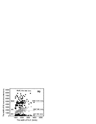
Figure 8: The widths of the Fe II lines compared to the widths of H$\beta$ components (upper, the sample of 111 AGN) and H$\alpha$ (bottom, the sample of 58 AGN); On X-axis are widths of Fe II, and on Y-axis are the widths of the NLR (triangles), ILR (circles) and VBLR (squares) components of H$\beta$ (H$\alpha$). Dotted, vertical line shows the average value of Fe II widths, while dotted, horizontal lines show the average values of the H$\beta$ (H$\alpha$) components. The average value of Fe II lines is the same or very close to average width value of ILR components of H$\beta$ and H$\alpha$.

In order to investigate the geometrical place of the Fe II emission region in AGN, we analyzed kinematical connection between the Fe II and Balmer emission region by comparing the line shifts and widths, obtained from the best-fitting. We assume that the broadening of the lines is caused by the Doppler effect from the random velocities of emission clouds, while the shift of the line is caused by the systemic motion of the emission gas. The results are presented in Fig. 8-9.

Figure 9: The correlation between the Fe II widths and widths of the H$\beta$ ILR components (left), H$\alpha$ ILR components (middle) and H$\alpha$ VBLR components (right). In all cases, correlations are observed (0.67, 0.72, 0.62), indicating kinematical connection between these emission regions.

The widths of the Fe II and H$\beta$ (upper) and H$\alpha$ (bottom) lines are compared in Fig. 8. The X-axis gives the Fe II line widths, while the Y-axis gives the parameters of the widths of the H$\beta$ (upper) and H$\alpha$ (bottom) components: the NLR (triangles), ILR (circles) and VBLR (squares). Dotted lines show the averaged values of widths: Fe II (vertical line) and H$\beta$ and H$\alpha$ line components (horizontal lines). On the sample of the 111 AGN that contain the H$\beta$ line (upper), the average value of Fe II widths is $1770\pm 580$ km/s, while the average values for H$\beta$ components are: $310\pm 160$ km/s (NLR), $1850\pm 660$ km/s (ILR) and $4690\pm 1210$ km/s (VBLR). Considering the selected sample of 58 AGN which have the H$\alpha$ line (bottom) the averaged value of the Fe II width is $1770\pm 570$ km/s and for the H$\alpha$ components: $270\pm 130$ km/s (NLR), $1470\pm 620$ km/s (ILR) and $4070\pm 1080$ km/s (VBLR). It is obvious that the averaged Fe II width ($1770$ km/s) is very close to the averaged widths of the ILR component of both the H$\beta$ and H$\alpha$ line (1850 km/s and 1470 km/s, respectively), while the averaged widths of the NLR and VBLR components are significantly different.

Fig. 9 shows the correlation between the Fe II widths and the H$\beta$ ILR ones ($r=0.67$, $p_{0}<0.0001$). Considering the H$\alpha$ ILR component, correlation is stronger, and it is $r=0.72$, $p_{0}<0.0001$. We have also found that a weaker correlation between widths of the Fe II and H$\alpha$ VBLR component ($r=0.55$, $p_{0}<0.0001$) is present. Relations between the shifts of Fe II and H$\alpha$ and H$\beta$ (NLR, ILR and VBLR components) are also investigated. It is noticed a positive correlation with the shift of the H$\alpha$ ILR component ($r=0.51$, $p_{0}<0.0001$). There is no a significant correlation between the Fe II shift and other H$\alpha$ and H$\beta$ components.

Boroson & Green (1992) found negative trend between the equivalent width (EW) of Fe II and [O III] lines ($r=-0.39$), as well as the anticorrelation between the EW Fe II and EW ([O III])/EW (H$\beta$) ($r=-0.53$). Thus, we tested the same relations on our sample of 111 AGN. We found slightly lower correlations then the previous authors: for EW Fe II vs. EW [O III] the correlation coefficient is $r=-0.26$ ($p_{0}=0.007$) and for EW Fe II vs. EW ([O III])/EW (H$\beta$) it is $r=-0.37$ ($p_{0}<0.0001$).

Then, we divided our initial sample of 111 AGN (0$<$z$<$0.7) in 6 subsamples, which are made by gradually removing the objects with low redshift in 6 steps. Subsamples contain object with redshifts in intervals: 0.1$<$z$<$0.7, 0.2$<$z$<$0.7, 0.3$<$z$<$0.7, 0.4$<$z$<$0.7, 0.5$<$z$<$0.7 and 0.6$<$z$<$0.7. Relation between EW Fe II and EW [O III] (also EW [O III]/EW H$\beta$) are analyzed separately for each subsample (see Table 2). We found that negative trend (r = - 0.37, P$<$0.0001) observed between EW Fe II and EW [O III]/EW H$\beta$ in initial sample (0$<$z$<$0.7), progress to significant anticorrelation (r$\sim$ - 0.70, P$<$0.0001) as we are removing low-redshift objects. The redshift dependance of the EW Fe II vs. EW [O III] anticorrelation may indicate some cosmological repercussion of the Fe II emission in AGN or dependence on luminosity.

Table 2: Correlations between equivalent widths (EW) of the Fe II and [O III] ([O III]/H$\beta$) lines for subsamples within different redshift intervals. Relation is fitted with function $Y=A+B\cdot X$. The coefficient of correlations r, the corresponding measure of the significance of correlations $p_{0}$, as well as the A and B coefficients, are shown in the table. In the last column, the number of objects in each subsample is given.

vs.		EW [O III]	EW [O III]/EW H$\beta$	No
EW FeII	$r$	-0.26	-0.37	109
(0$<$z$<$0.7)	$p_{0}$	0.007	$<0.0001$
EW FeII	$r$	-0.30	-0.40	92
(0.1$<$z$<$0.7)	$p_{0}$	0.004	$<0.0001$
EW FeII	$r$	-0.42	-0.50	74
(0.2$<$z$<$0.7)	$p_{0}$	2.2E-4	$<0.0001$
EW FeII	$r$	-0.44	-0.56	58
(0.3$<$z$<$0.7)	$p_{0}$	6.0E-4	$<0.0001$
EW FeII	$r$	-0.56	-0.62	43
(0.4$<$z$<$0.7)	$p_{0}$	$<0.0001$	$<0.0001$
EW FeII	$r$	-0.64	-0.70	28
(0.5$<$z$<$0.7)	$p_{0}$	2.37E-4	$<0.0001$
EW FeII	$r$	-0.68	-0.72	14
(0.6$<$z$<$0.7)	$p_{0}$	0.007	0.004

5 Results and discussion

In this progress report we give some results of our recent investigations of different broad line parameters (the flux ratios, EW, FWHM, etc.) in order to probe the physics of the ELR, i.e. the hydrogen Balmer lines (H$\alpha$ to H$\varepsilon$), the helium lines from two subsequent ionization levels (He II $\lambda$4686 and He I $\lambda$5876) and the strongest Fe II lines in the wavelength interval $\lambda\lambda 4400-5400\AA$.

From the analysis of the hydrogen Balmer lines, we can say that the BP method gives valid results if the error of the BP fit $f$ is less than 10% (eventually 20% in the measured spectra). The parameter space of CLOUDY simulations where $f<10\%$ is well constrained and in a similar range for different column densities $N_{\rm H}$ (Fig. 2). This area of parameters contains lower ionizing fluxes and higher hydrogen densities, but depending on the column density the area increases keeping the same trend between the $n_{\rm H}$ and $\Phi_{\rm H}$, Therefore, for those parameters the BP method could be applied for the estimation of the excitation temperature. This indicates that for some physical conditions, even if we have the photoionization as the main heating process in the BLR, the hydrogen Balmer lines are produce in such way that they obey the Saha-Boltzmann equation, i.e. the BLR plasma is at least in the Partial Local Thermodynamical Equilibrium.

The physical parameters of the simulations for which the BP method could be applied ($f<10\%$) follow some relations even when the column density changes. There is a linear relation between the average temperature $T_{\rm av}$ of the emitting region and helium lines ratio $R$: $T_{\rm av}=A+B\cdot R$ (Fig. 4, Table 1). Also, the hydrogen density depends on the helium line ratio $R$ as: $\log n_{H}=D/(C+R)$, where $n_{H}$ is given in the units of $10^{7}{\rm cm^{-3}}$ (Figure 4, Table 1). For lower column densities ($N_{\rm H}=10^{21}-10^{22}\rm cm^{-2}$) this linear trend for $T_{\rm av}$ seems to be broken after some value of $R$ (Fig. 4, upper), therefore the results obtained for this column densities should be taken with caution. The ranges of the average temperature and hydrogen density, obtained when these relations are applied to the observed sample of AGN taken from the SDSS database, are in good agreement with the previous estimates of the physical conditions in the BLR (Osterbrock & Ferland, 2006). Having in mind problems given in §2.1 (i.e. different emitting regions of helium and Balmer lines or the multicomponent origin of BELs) the relations given in Table 1 could be use as a rough estimate of the BLR physical parameters from direct measurements.

On the other hand, from the analysis of the Fe II emission, we found the significant correlation between the Fe II and H$\alpha$, H$\beta$ ILR widths which indicate the ILR origin of the Fe II emission. Also, the Fe II emission region is mainly characterized with random velocity of $\sim$1800 km/s, that corresponds to the ILR origin. This result is in favor to the results obtained by Popović et al. (2004), and with the recent findings that the optical Fe II line forming region seems to not be the same as the BLR (Kuehn et al., 2008; Hu et al., 2008; Popović et al., 2009). Moreover, we found that the degree of anticorrelation of EW Fe II - EW [O III] (EW [O III]/H$\beta$) is redshift dependent, i.e. anticorrelation increases by selection of the sample with high redshift objects.

6 Conclusions

We used here the emission lines to estimate the physical parameters of the BLR and properties of the Fe II line forming region. From our investigations we can outline the following conclusions:

1. In the case of the pure photoionized plasma, there can exist the conditions that the excitation of the hydrogen Balmer lines is sensitive to the temperature. In this case, the He II/He I line ratio can be used for the estimates of the averaged temperature and hydrogen density. This can be very useful for determining the physical properties of the BLR, and for a small sample of AGN we found that the BLR temperatures are ranging from $\sim$ 5000 K to 18000 K, and hydrogen densities from 10⁸ cm^-3 to 10¹² cm^-3. These values of the temperature and density are expected in the BLR plasma (Osterbrock & Ferland, 2006).

2. The optical Fe II emission is likely coming from a region that corresponds to the ILR. Also, there is a weak correlation with the VBLR component of Balmer lines indicating that a fraction emitted in the Fe II lines can originate also in the BLR. On the other hand, the correlation between the EW FeII and EW [OIII] (EW[OIII]/EW H$\beta$) discovered by Boroson & Green (1992) seems to be sensitive on redshift (or luminosity) of AGN.

Finally, the BLR physics (and geometry) still remains an open question, and we hope that with this work we approached some conclusions which will help us in understanding the BLR physics.

Acknowledgments

D.I. would like to thank to the Department of Astronomy of the University of Padova in Italy for their hospitality. This work was supported by the Ministry of Science of Serbia through the project Astrophysical Spectroscopy of Extragalactic Objects (#146002).

Funding for the SDSS and SDSS-II has been provided by the Alfred P. Sloan Foundation, the Participating Institutions, the National Science Foundation, the U.S. Department of Energy, the National Aeronautics and Space Administration, the Japanese Monbukagakusho, the Max Planck Society, and the Higher Education Funding Council for England. The SDSS is managed by the Astrophysical Research Consortium (ARC) for the Participating Institutions. The SDSS Web Site is http://www.sdss.org/. This research has made use of NASA’s Astrophysics Data System.

References

- Boroson & Green (1992) Boroson T. A. & Green R. F., 1992, ApJS, 80, 109
- Dumont, Collin-Souffrin & Nazarova (1998) Dumont A.-M., Collin-Souffrin S., Nazarova L., 1998, A&A, 331, 11
- Ferland (2006) Ferland G. J., 2006, Hazy, A Brief Introduction to Cloudy 06.02, University of Kentucky Internal Report
- Ferland et al. (1998) Ferland G. J., Korista K. T., Verner D. A., Ferguson J. W., Kingdon J. B., Verner E. M., 1998, PASP, 110, 761
- Griem (1997) Griem H. R. 1997, Principles of plasma spectroscopy, Cambridge: Cambridge University Press
- Hu et al. (2008) Hu C., Wang J.-M., Ho L. C., Chen Y.-M., Zhang H.-T., Bian W.-H., Xue S.-J. 2008, ApJ, 687, 78
- Korista & Goad (2000) Korista, K. T., Goad, M. R. 2000, ApJ, 536, 284
- Korista & Goad (2004) Korista K. T., Goad M. R. 2004, ApJ, 606, 749
- Kuehn et al. (2008) Kuehn C. A., Baldwin J. A., Peterson B. M., Korista K. T. 2008, ApJ, 673, 69
- La Mura et al. (2007) La Mura G., Popović L. Č., Ciroi S., Rafanelli P., Ilić D. 2007, ApJ, 671, 104
- Osterbrock & Ferland (2006) Osterbrock D. E., Ferland G. J., 2006, Astrophysics of Gaseous Nebulae and Active Galactic Nuclei (2nd ed.), University Science Books, Sausalito, California
- Popović (2003) Popović L. Č., 2003, ApJ, 599, 140
- Popović (2006a) Popović L. Č., 2006a, ApJ, 650, 1217 (an Erratum)
- Popović (2006b) Popović L. Č., 2006b, SerAJ, 173, 1
- Popović et al. (2004) Popović L. Č., Mediavilla E. G., Bon E., Ilić D., 2004, A&A, 423, 909
- Popović et al. (2008) Popović L. Č., Shapovalova A. I., Chavushyan V. H., Ilić D., Burenkov A. N., Mercado A., Ciroi S., Bochkarev N. G., 2008, PASJ, 61, 1
- Popović et al. (2009) Popović L. Č., Smirnova A. A., Kovačević J., Moiseev A. V., Afanasiev V. L. 2009, AJ, 137, 3548
- Shapovalova et al. (2008) Shapovalova A. I., Popović L. Č., Collin S., Burenkov A. N., Chavushyan V. H. et al., 2008, A&A, 486, 99
- Sulentic et al. (2000) Sulentic J. W., Marziani P., Dultzin-Hacyan D., 2000, ARA&A, 38, 521