Ultrahigh Purcell factors and Lamb shifts using slow-light metamaterial waveguides

Abstract

Employing a medium-dependent quantum optics formalism and a Green function solution of Maxwell’s equations, we study the enhanced spontaneous emission factors (Purcell factors) and Lamb shifts from a quantum dot or atom near the surface of a slow-light metamaterial waveguide. Purcell factors of approximately 250 and 100 are found at optical frequencies for $p-$polarized and $s-$polarized dipoles respectively placed 28 nm (0.02 $\lambda_{0}$) above the slab surface, including a realistic metamaterial loss factor of $\gamma/2\pi=2\,\mathrm{THz}$. For smaller loss values, we demonstrate that the slow-light regime of odd metamaterial waveguide propagation modes can be observed and related to distinct resonances in the Purcell factors. Correspondingly, we predict unusually large and rich Lamb shifts of approximately $-1$ GHz to $-6$ GHz for a dipole moment of 50 Debye. We also make a direct calculation of the far field emission spectrum which contains direct measurable access to these enhanced Purcell factors and Lamb shifts.

I Introduction

Early in 1968, Veselago predicted that a planar slab of negative-index material (NIM), which possesses both negative permittivity $\varepsilon$ and negative permeability $\mu$, could refocus electromagnetic waves veselago . While an interesting prediction, these so-called metamaterials did not receive much attention in optics research until Sir John Pendry showed that NIMs could be used as a “superlens”, which could overcome the diffraction limit of conventional imaging system pendry . Subsequently, a host of applications has been proposed, ranging from designs for optical cloaks to hide objects pendry2006 , through to schemes that completely stop light kosmas . Although most of these schemes are idealized, and suffer in the presence of metamaterial loss, they have nevertheless motivated significant experimental progress. For example, Schurig et al. experimentally demonstrated some cloaking features by split-ring resonators schurig ; and recent achievements in fabrication have facilitated the realization of negative indices at communication wavelength dolling , with some extension to quasi-3D structures also reported valentine .

While it is certainly becoming established that metamaterials posses some remarkable classical optical properties, less well studied are their quantum optical properties, such as what happens to the spontaneous emission of an embedded atom or quantum dot. In 1946, Purcell pointed out that due to the spatial variation of the local photon density of states (LDOS), the spontaneous emission rate in a cavity can be enhanced or suppressed depending upon the distance between the mirrors purcell . The modification of spontaneous emission due to inhomogeneous structures is a large field in its own right, leading to applications in quantum optical technology singlePhotons . In the domain of metamaterials, Kästel and coworkers investigated the spontaneous emission of an atom placed in front of a mirror with a layer of NIM kastel ; this study was motivated by the perfect lens prediction of a vanishing optical path length between the focal points, leading to the peculiar property that the evanescent waves emerging from the source are exactly reproduced; consequently they found that the spontaneous emission can be completely suppressed. This prediction does not account for the essential inclusion of metamaterial loss or absorption; yet, it is well known that metamaterials must be dispersive and absorptive to satisfy the fundamental principle of causality and the Kramers-Krönig relation stockman . Not surprisingly, when absorption is necessarily taken into account, then the predicted properties of an ideal lossless metamaterial can qualitatively change. For example, the superlens and the invisible cloak are never perfect smith ; yao , and slow light modes can never be really stopped and are usually impractically lossy arvin . Similarly, it is expected that absorption will have an important influence on the modification of spontaneous emission sambale . In this regard, Xu et al. have extended the works of Kästel et al. to one dimensional right-handed and left-handed material layers and find that nonradiative decay and instantaneous radiative decay will certainly weaken the predicted inhibition of spontaneous emission xu2006 ; xu2007 .

Some of the first theories to treat quantum electrodynamics near a interface were introduced around 1984 by Wylie and Sipe SipePRA1984 ; SipePRA1985 , where, using Green function techniques, they showed that the scattered field can be expressed in terms of the appropriate Fresnel susceptibilities. Using such methods, it is now well known that the photonic LDOS can be increased near a metallic surface, e.g. see Ref. JoulainPRB2003 , whereby the $p-$polarized dipole couples to a transverse magnetic (TM) surface plasmon polariton (SPP). Typically such resonances are far from the optical frequency domain and they are restricted to TM polarization; in addition, the emission is dominated by quenching or non-radiative decay. Even in the presence of gratings, enhanced emission via SPPs is not very practical SunAPL2007 . However, the rich waveguide properties of metamaterials have quite different polarization dependences and mode structures than SSPs at a metal surface; for example, they can support slow-light, bound propagation modes and transverse electric (TE or $s-$polarized) SPPs.  It is therefore of fundamental interest to explore the quantum optical aspects of these novel waveguides.

Enhanced emission at the surface of both metals and metamaterial slabs was studied in 2004 by Ruppin and Martin RuppinMartin2004 .  They noted that resonance peaks due to $s-$polarized surface modes and waveguide modes can appear for the metamaterial case, although they did not discuss the origin of the waveguide peaks. Similar findings were found by Xu et al. XuPRA2009 , but the role of loss was not explored in detail but rather it was treated as a perturbation and assumed to lead to only dissipation; such an assumption is highly suspect in a NIM waveguide, since the entire modal characteristics of the structure depend intimately upon the material loss and dispersion profiles arvin . Very recently, spontaneous emission enhancements in NIM materials and interesting quantum interference effects have been reported by Li et al. LiPEB2009 , although unrealistically small losses were typically assumed, and again the physics behind the enhancement factors was not made clear. In all of these works, there has been no quantitative connection made to the complex band structure or to the far-field (and thus measurable) spontaneous emission spectra or dipolar frequency shifts (Lamb shifts).

In this work, the modified spontaneous emission of a quantum dot or atom (single photon emitter) situated above a slow-light metamaterial waveguide is investigated in detail by employing a medium-dependent Green function theory and comparing with the lossy guided waveguide modes. We compute the PF as well as the spontaneous emission spectrum in the far field by developing and using a rigorous quantum optics theory. We stress that the recent prediction of completely stopped waveguide modes in a metamaterial waveguide kosmas would lead to an infinite PF, but as reported by Reza et al. arvin , the properties of the slow-light modes are significantly changed in the presence of loss; thus we also investigate the dependence on loss in some detail. We show that the emission properties of a photon emitter can act as a probe for below light-line propagation mode characteristics, showing measurable enhanced radiative broadening and quantum Lamb shifts. The Lamb shifts are found to be extremely rich and pronounced. We also compare and contrast these NIM quantum optical features with well known results for metallic surfaces.

Our paper is organized as follows. In Sect. II, we introduce the NIM waveguide structure of interest and compute and discuss the band structure for both $s$ (TE) and $p$ (TM) polarization. In Sect. III, we present a rigorous theory for calculating the Purcell factor (PF), Lamb shift, and emitted spectrum from a single photon emitter. From this theory, we derive an explicit and analytical solution to the emitted field at any spatial location using a full non-Markovian theory which is valid for any general media (lossy and inhomogeneous). In Sect. IV, we discuss a general technique for computing the multi-layered Green function using a stratified medium technique of Paulus et al. Paulus-PRE-62-5797 , and formally separate the total Green function into a homogeneous and scattered part to properly obtain the photonic Lamb shift. In Sect. V, we present calculations for the Purcell effect and Lamb shift, as well as the spontaneous emission spectra emitted into the far field. Finally, we give our conclusions in Sect. VI.

II Metamaterial slab waveguides: complex band structure and slow-light propagation modes

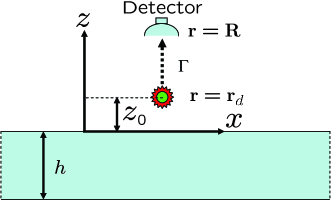
Figure 1: Schematic diagram of the system being investigated.  The green dot at ${\bf r}={\bf r}_{d}$ refers to the atom or quantum dot that is decaying radiatively (with a rate $\Gamma$), at a distance $z_{0}$ above the slab of thickness $h$. The vertical position of the dot, $z_{d}=z_{0}$.

In the following sections, we wish to calculate the spontaneous emission from dipoles $\mathrm{\mathbf{d}}=d{\mathbf{e}}_{\alpha}$, where $\alpha=z$ or $\alpha=x(y)$.  Because the spontaneous emission is strongly affected by the metamaterial waveguide modes, in this section we present the results of calculations of the dispersion of both TE and TM propagation modes.  The schematic diagram of the system under study is shown in Fig. 1. The negative index slab is surrounded by air and assumed infinite (or much larger than a wavelength) in the $x$ and $y$ directions. The thickness of the slab is $h=280\,$nm. In view of the importance of dispersion and absorption, we take both into account from the beginning, which ensures causality and thus avoids unphysical results. The dispersion is introduced via the Lorentz and Drude models taflove :

$$\mu(\omega) = 1+\frac{\omega_{pm}^{2}}{\omega_{0}^{2}-\omega^{2}-i\gamma\omega},$$ (1)

$$\varepsilon(\omega) = 1-\frac{\omega_{pe}^{2}}{\omega^{2}+i\gamma\omega},$$ (2)

where $\omega_{pm}$ and $\omega_{pe}$ are the magnetic and electric plasmon frequencies, and $\omega_{0}$ is the atomic resonance frequency. In what follow, we are interested in waveguides with guided modes at optical frequencies and thus take $\omega_{0}/2\pi=189.4\,\mathrm{THz}$, $\omega_{pm}/2\pi=165.4\,\mathrm{THz}$, $\omega_{pe}/2\pi=490\,\mathrm{THz}$.

To solve the complex band structure, one can work with a complex wave vector ($\beta$) and a real frequency ($\omega$), or, alternatively, a complex$-\omega$ and a real$-\beta$. The former is perhaps more appropriate for modeling plane wave excitation, while the latter is better suited for a broadband excitation response that is invariant in $z$. Neither of these approaches constitutes a complete connection to a broadband dipole response, and thus we will show both solutions, and briefly discuss their main features. The details of these two approaches for modelling metamaterial waveguide properties will be presented elsewhere.

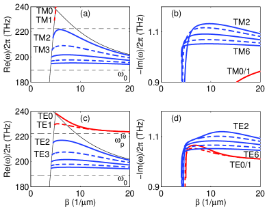
Figure 2: Dispersion curves of the lossy metamaterial waveguide for the first few lower-order modes using the complex-$\omega$ approach for $\gamma/2\pi=2\,$THz ($\gamma/\omega_{0}\approx 0.01$). The red and blue curves show the surface plasmon polariton modes and bound propagation modes, respectively.  The solid and dashed curves represent the even and odd modes, respecitvely. The solid thick black curves display the vacuum light-line and metamaterial light-line, while the horizontal dashed lines indicate the atomic ($\omega_{0}$) and TE plasmon resonances ($\omega_{p}^{\mathrm{te}}$). (a) $\mathrm{Re(\omega)}$ versus $\beta$ for TM modes. The modes become more dense near the resonance frequency $\mathrm{\omega_{0}}$, and form a continuum. (b) $\mathrm{Im(\omega)}$ versus $\beta$ for TM modes. (c)(d) The same as (a)(b) but for TE modes.

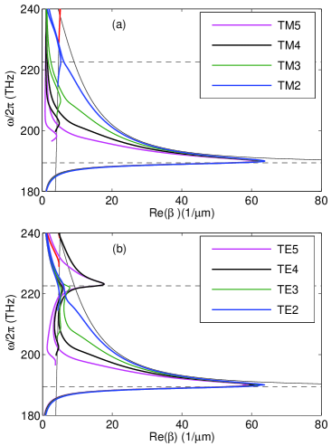
Figure 3: Dispersion curves of the lossy metamaterial waveguide for the first few lower-order modes in using the complex-$\beta$ approach, where only $\mathrm{Re}[\beta]$ is shown. (a) TM modes. (b) TE modes. The thin solid black curves represent vacuum light-line and metamaterial light-line. Note that formally labelling the curves is more difficult than in Fig. 2 due to the merging of the different curves (e.g. the TM1 and TM5 curves near 220 THz).

The complex dispersion curves of the aforementioned metamaterial waveguide for both TE and TM modes are shown in Fig. 2 and Fig. 3, using complex-$\omega$ and complex-$\beta$ approaches, respectively. In the complex$-\beta$ approach, we only show the $\mathrm{Re}[\beta]$ solution (Fig. 3), as the $\mathrm{Im}[\beta]$ simply demonstrates the large losses in the regime of slow light arvin . These curves come from the complex solution to the transcendental dispersion equation derived from the Maxwell’s equations and the guidance conditions key-1 .

In Fig. 2, we show the first few TM (TE) propagation modes: TM2-TM6 (TE2-TM6), as well as TE0-TE1 (TM0-TE1) SPP modes (red curves); a wide range of frequencies is displayed from from 180 to 240 THz. We stress that the TE-polarized SPPs are unique to metamaterials and the properties of these SSP modes can be engineered to have a resonance in the optical frequency regime, near the propagation modes. For the TM case, there is also a higher-lying SPP resonance, which we do not show as it is far outside the frequency of interest ($\omega_{sp}^{\mathrm{tm}}\sim 346$ THz   or specifically $\omega_{pe}/\sqrt{2}$); the TM0 and TM1 modes show the start of the SPP modes just below the air light line.

The properties of these metamaterial waveguide modes shown in Fig. 2 are considerably different from those in a conventional dielectric waveguide key-2 . The most important difference is that backward and forward propagating modes exist and, in a lossless metamaterial waveguide, even stopped-light modes (where the slope goes to zero) are supported. However, the necessary inclusion of intrinsic loss in a metamaterial slab dramatically changes the dispersion curves near slow-light regions (see also Ref. arvin ). Thus one must include material losses to have any confidence in the results and predictions. In the complex$-\omega$ solutions (Fig. 2), although the slope and thus the group velocity $v_{g}$ is zero at some points, the use of the group velocity as a measure of energy transport is not meaningful arvin , and there is a finite imaginary part of frequency. We note, however, that at the points where the slope is zero in Fig.  2(a) and (c), the density of modes is large and as we shall see, this can lead to a large Purcell factor at the relevant frequencies. We note in particular that because the slope of all of the different mode dispersions tends to zero as $\beta$ goes to infinity, there is a large enhancement in the density of states at $\omega=\omega_{0}$.

In Fig. 3 we show the dispersion curves using the complex$-\beta$ approach. In this approach, the impact of material losses on the dispersion curves are much more drastic and these curves would appear to have little to do with the curves in Fig. 2. However, despite their differences, there is a strong correspondence between the two sets of curves. In a (fictitious) lossless waveguide, the two sets of curves would be identical apart from some leaky modes that carry no energy. In the complex$-\beta$ approach, two degenerate leaky modes start at the zero-slope point of the non-SSP propagation modes and move to higher frequencies. In Fig. 2, these leaky modes split and merge seamlessly into the propagation mode dispersion, creating the split-curve structure that is seen, e.g. for the TE4 mode near $\omega/2\pi=201\,$THz. Although the slope no longer goes to zero in the complex$-\beta$ approach at the point where the propagation mode splits into the two leaky modes, the energy velocity (which is the correct measure of energy transport in a lossy system) is quite small but nonzero. Another important difference between the modes in the complex$-\beta$ approach and the complex-$\omega$ approach is that for the modes in the complex$-\omega$ approach, $\beta\rightarrow\infty$ as $\omega\rightarrow\omega_{0}$, while in the complex$-\beta$ approach, the modes bend back on themselves at the atomic resonance frequency $\omega_{0}$. Note that the group velocity, which is given by the slope of dispersion curve, is infinite at this point. There is no paradox here because, as discussed above, the group velocity is ill-defined in a lossy waveguide structure and the energy velocity is a correct measure of the transport speed key-4 . We have calculated the energy velocity and find that the minimum energy velocity occurs exactly at the resonance frequency $\omega_{0}$, but that it is never zero; for example, the energy velocity minimum for both TE3 and TM3 modes is found to be around $10^{-3}c$ to $10^{-4}c$, where $c$ is the vacuum speed of light. A similar effect occurs for TE modes near the plasmon resonance, where in the in the complex$-\beta$ picture, the SSP modes not only penetrate below the plasmon frequency, but they transform seamlessly into the higher-order leaky modes. For example, the TE4 and TE5 modes merge into SSP modes. Interestingly, in Fig. 3(b), we also observe new resonances in the left branch of the leaky TE propagation modes, which couple to the TE SPP modes just below the bare SPP resonance.  Thus, two resonances appear in this SPP frequency regime; evidently, this is not expected from the complex$-\omega$ perspective.

Later, we will show that the resonant frequency and the slow light regimes of the propagation modes are exactly coincident to that of the LDOS peaks in the spontaneous emission spectrum, and thus both complex$-\omega$ and complex$-\beta$ band structures are useful to gain insight into the origin of the LDOS peaks. The spatial symmetries of the even and odd modes will also prove to be very important; since the odd modes have a much larger field amplitude at the surface, they couple much more strongly to a quantum dot or atom near the NIM surface.

III Quantum theory of spontaneous emission in metamaterial

III.1 Purcell factor (PF) and Lamb shift

The PF is a measure of the spontaneous emission rate enhancement; it is defined as $PF={\Gamma}/{\Gamma_{0}}$, where $\Gamma$ (the Einstein A coefficient) is the spontaneous emission rate associated with population decay rate from an excited state to the ground state, and $\Gamma_{0}$ is the spontaneous emission rate in vacuum or a lossless homogeneous medium. We consider a system consisting of a quantum dot embedded in or near a general dispersive, absorptive, and inhomogeneous medium. Employing a quantization scheme that rigorously satisfies the Kramers-Krönig relations, and using the electric dipole approximation, an appropriate Hamiltonian – following the works of Welsch and coworkers – can be written as dung1 ; dung2 ; dungpra043816 :

$$H = \!\!\hbar\omega_{d}\hat{\sigma}^{+}\!\hat{\sigma}^{-}+\sum_{\lambda=e,m}\int d\mathbf{r}\int_{0}^{\infty}\!\!d\omega_{l}\hbar\omega_{l}\hat{\mathbf{f}}_{\lambda}^{\dagger}(\mathbf{r},\omega_{l})\cdot\hat{\mathbf{f}}_{\lambda}(\mathbf{r},\omega_{l})$$ (3)

$$- [\hat{\sigma}^{+}\mathbf{d}+\hat{\sigma}^{-}\mathbf{d}]\cdot\mathbf{F}(\mathbf{r}_{d}),$$

where $\hat{\mathbf{f}}_{\lambda}^{\dagger}(\mathbf{r},\omega_{l})$ and $\hat{\mathbf{f}}_{\lambda}(\mathbf{r},\omega_{l})$ are the continuum bosonic-field operators of the electric ($\lambda=e$) and magnetic field ($\lambda=m$) with eigenfrequency $\omega_{l}$, $\hat{\sigma}^{(\pm)}$ are the Pauli operators of the electron-hole pair (exciton), and $\omega_{d}$ and $\bm{d}=\bm{n}_{d}d$ ($d$ is assumed to be real) are the transition frequency and dipole moment of the dot, respectively.  The field operator $\hat{\mathbf{F}}$ is essentially the electric field operator augmented by the quantum dot polarization and can be expressed as $\hat{\mathbf{F}}=\hat{\mathbf{D}}/({\varepsilon_{0}\varepsilon})+{\hat{\mathbf{P}}}/({\varepsilon_{0}\varepsilon})$, where ${\hat{\mathbf{D}}}$ is the displacement field (${\hat{\mathbf{E}}}=\hat{\mathbf{D}}/({\varepsilon_{0}\varepsilon})$ is the electric field away from the dipole), ${\varepsilon}$ is the complex relative permittivity and ${\hat{\mathbf{P}}}$ is the polarization arising from the quantum dot dipole; this latter contribution is needed as it is the displacement field that should couple to the dipole in the interaction Hamiltonian HealyPRA1980 ; PowerPRA1982 ; SipePRA1984 . Using the above formalism, we derive

$$\hat{\mathbf{F}}(\mathbf{r},t) \!\!= i\sqrt{\frac{\hbar}{\pi\varepsilon_{0}}}\!\!\int_{0}^{\infty}\!\!\!d\omega_{l}\!\!\!\int\!\!d\mathbf{r}^{\prime}\mathbf{G}(\mathbf{r},\mathbf{r}^{\prime};\omega_{l})\cdot\left[\sqrt{\varepsilon_{I}(\mathbf{r}^{\prime},\omega_{l})}\right.$$ (4)

$$\left.\!\!\!\!\!\!\!\!\hat{\mathbf{f}}_{e}(\mathbf{r}^{\prime},\omega_{l};t)+\frac{c}{\omega_{l}}\nabla\times\sqrt{-\kappa_{I}(\mathbf{r}^{\prime},\omega_{l})}\,\hat{\mathbf{f}}_{m}(\mathbf{r}^{\prime},\omega_{l};t)\right]$$

$$\!\!\!\!\!+H.c.+\frac{{\bf d}[\hat{\sigma}^{+}(t)+\hat{\sigma}^{-}(t)]\,\delta({\bf r}-{\bf r}_{d})}{\varepsilon_{0}\varepsilon({\bf r})},$$

where the last term represents the polarization field from the dipole, $\varepsilon_{I}(\mathbf{r},\omega_{l})$ and $\kappa_{I}(\mathbf{r},\omega_{l})$ are the imaginary parts of $\varepsilon(\mathbf{r},\omega_{l})$ and $1/\mu(\mathbf{r},\omega_{l})$ respectively, and $\varepsilon(\mathbf{r},\omega_{l})$ and $\mu(\mathbf{r},\omega_{l})$ are the relative complex permittivity and permeability. The dyadic $\mathbf{G}(\mathbf{r},\mathbf{r}^{\prime};\omega_{l})$ is the electric-field Green function (GF) that describes the field response at $\mathbf{r}$ to an oscillating polarization dipole at $\mathbf{r}^{\prime}$ as a function of frequency; the GF is defined from

$$\!\!\!\!\!\!\!\!\left[{\nabla}\!\times\!\frac{1}{\mu(\omega_{l},\mathbf{r})}{\nabla}\!\times\!-\frac{\omega_{l}^{2}}{c^{2}}\varepsilon(\omega_{l},\mathbf{r})\right]\textbf{G}(\mathbf{r},\mathbf{r}^{\prime};\omega_{l})=$$

$$\frac{\omega_{l}^{2}}{c^{2}}{\bf 1}\,\delta({\bf r}-{\bf r}^{\prime}),$$ (5)

where ${\bf 1}$ is the unit tensor.

From the above Hamiltonian, we derive the Heisenberg equations of motion for the time-dependent operator equations as ($t$ is implicit):

$$\frac{d\hat{\sigma}^{-}}{dt}=-i\omega_{l}\hat{\sigma}^{-}+i\hbar^{-1}\mathbf{d}\cdot\hat{\mathbf{F}}(\mathbf{r}_{d}),$$ (6)

$$\frac{d\hat{\mathbf{f}}_{e}(\mathbf{r},\omega_{l})}{dt}=-i\omega_{l}\hat{\mathbf{f}}_{e}(\mathbf{r},\omega_{l})$$

$$\qquad\qquad-\sqrt{\frac{\varepsilon_{I}(\mathbf{r},\omega_{l})}{\pi\hbar\varepsilon_{0}}}\bm{d}\cdot\mathbf{G}^{*}(\mathbf{r}_{d},\mathbf{r};\omega_{l})[\hat{\sigma}^{-}+\hat{\sigma}^{+}],$$ (7)

$$\frac{d\hat{\mathbf{f}}_{m}(\mathbf{r},\omega_{l})}{dt}=-i\omega_{l}\hat{\mathbf{f}}_{m}(\mathbf{r},\omega_{l})$$

$$\!\!\!\!\!\!\!\!\!\!\!\!\!\!\!\!\qquad\qquad-\sqrt{\frac{-\kappa_{I}(\mathbf{r},\omega_{l})}{\pi\hbar\varepsilon_{0}}}\frac{c}{\omega_{l}}\bm{d}\cdot[\mathbf{G}^{*}(\mathbf{r}_{d},\mathbf{r};\omega_{l})\times\nabla][\hat{\sigma}^{-}+\hat{\sigma}^{+}],$$

where $[\mathbf{G}^{*}(\mathbf{r}_{d};\mathbf{r};\omega_{l})\times\nabla]_{ij}=\epsilon_{jkl}\partial_{k}{G}_{il}^{*}(\mathbf{r}_{d},\mathbf{r};\omega_{l})$, and we have used the one photon or weak excitation approximation through $\hat{\sigma}_{z}\hat{\mathbf{F}}=-\hat{\mathbf{F}}$. We can make a Laplace transform on the above set, defined through $\hat{O}_{i}(\omega)=\int_{0}^{\infty}e^{i\omega t}\hat{O}_{i}(t)dt$, and obtain

$$\hat{\sigma}^{-}(\omega) = \frac{i\hat{\sigma}^{-}(t=0)}{\omega-\omega_{d}}-\frac{\hbar^{-1}\mathbf{d}\cdot\hat{\mathbf{F}}(\mathbf{r}_{d},\omega)}{\omega-\omega_{d}},$$ (9)

$$\hat{\sigma}^{+}(\omega) = \frac{i\hat{\sigma}^{+}(t=0)}{\omega+\omega_{d}}+\frac{\hbar^{-1}\mathbf{d}\cdot\hat{\mathbf{F}}(\mathbf{r}_{d},\omega)}{\omega+\omega_{d}},$$ (10)

$$\hat{\mathbf{f}}_{e}(\mathbf{r},\omega_{l};\omega) = \hat{\mathbf{f}}_{e}^{0}(\mathbf{r},\omega_{l};\omega)$$

$$\!\!\!\!\!\!\!\!\!\!\!\!\!\!\!-\sqrt{\frac{\varepsilon_{I}(\mathbf{r},\omega_{l})}{\pi\hbar\varepsilon_{0}}}\mathbf{d}\cdot\mathbf{G}^{*}(\mathbf{r}_{d},\mathbf{r};\omega_{l})\frac{i[\hat{\sigma}^{-}(\omega)+\hat{\sigma}^{+}(\omega)]}{\omega-\omega_{l}},$$

$$\hat{\mathbf{f}}_{m}(\mathbf{r},\omega_{l};\omega) = \hat{\mathbf{f}}_{m}^{0}(\mathbf{r},\omega_{l};\omega)$$ (12)

$$\!\!\!\!\!\!\!\!\!\!\!\!-\sqrt{\frac{-\kappa_{I}(\mathbf{r},\omega_{l})}{\pi\hbar\varepsilon_{0}}}\frac{c}{\omega_{l}}\mathbf{d}\cdot[\mathbf{G}^{*}(\mathbf{r}_{d},\mathbf{r};\omega_{l})\times\nabla]$$

$$\frac{i[\hat{\sigma}^{-}(\omega)+\hat{\sigma}^{+}(\omega)]}{\omega-\omega_{l}},$$

where $\mathbf{f}^{0}$ represents a possible free field or homogeneous driving field in the absence of any quantum dot or atom.

We next assume that the initial field is the vacuum field (${i.e.}$, $\hat{\mathbf{f}}_{\lambda}^{0}(\mathbf{r},\omega_{l};\omega)=0$), substitute Eqs.(III.1-12) into Eq.(4), and make use of the relation (see dungpra043816 ):

$$\int d\mathbf{s}\{-\kappa_{I}[\mathbf{G}(\mathbf{r},\mathbf{s};\omega_{l})\times\nabla_{s}][\nabla_{s}\times{\bf G}^{*}(\mathbf{s},\mathbf{r^{\prime}};\omega_{l})]\frac{c^{2}}{\omega_{l}^{2}}+$$

$$\varepsilon_{I}(\mathbf{s},\omega_{l})\mathbf{G}(\mathbf{r},\mathbf{s},\omega_{l})\cdot{\bf G}^{*}(\mathbf{s},\mathbf{r^{\prime}};\omega_{l})\}=\rm Im\mathbf{G}(\mathbf{r},\mathbf{r^{\prime}};\omega_{l}).\ \$$ (13)

Subsequently, we obtain an explicit solution for the dipole operators (and thus the polarization operator):

$$\hat{\sigma}^{-}(\omega)+\hat{\sigma}^{+}(\omega)=$$

$$\!\!\!\!\!-\frac{i\hat{\sigma}^{-}(t=0)(\omega+\omega_{d})+i\hat{\sigma}^{+}(t=0)(\omega-\omega_{d})}{\omega_{d}^{2}-\omega^{2}-2\omega_{d}\,\mathbf{d}\cdot{[\mathbf{G}}(\mathbf{r}_{d},\mathbf{r}_{d};\omega)+\frac{\delta(\mathbf{r}-\mathbf{r}_{d})}{\varepsilon({\bf r})}]\cdot\mathbf{d}/\hbar\varepsilon_{0}},$$

which we can rewrite as

$$\hat{\sigma}^{-}(\omega)+\hat{\sigma}^{+}(\omega)=$$

$$\ \ \ \ \ -\frac{i\hat{\sigma}^{-}(t=0)(\omega+\omega_{d})+i\hat{\sigma}^{+}(t=0)(\omega-\omega_{d})}{\omega_{d}^{2}-\omega^{2}-2\omega_{d}\,\mathbf{d}\cdot{\mathbf{K}}(\mathbf{r}_{d},\mathbf{r}_{d};\omega)\cdot\mathbf{d}/\hbar\varepsilon_{0}},\ \ \ \ \$$ (15)

where the new GF, $\mathbf{K}(\mathbf{r},\mathbf{r}^{\prime};\omega)\equiv\mathbf{G}(\mathbf{r},\mathbf{r}^{\prime};\omega)+\delta(\mathbf{r}-\mathbf{r}^{\prime})/\varepsilon(\mathbf{r})$. This is exactly the same form as the GF used in the formalism by Wubs et al. wubs04 , where the $\mathbf{K}$ function appears naturally when working with mode expansion techniques for lossless inhomogeneous media. The origin of the discrepancy between theories that use $\mathbf{G}$ or $\mathbf{K}$, is because the correct interaction Hamiltonian should really contain a displacement field HealyPRA1980 ; PowerPRA1982 ; SipePRA1984 , as has been accounted for in our Eq. (4). This subtlety becomes important, e.g., when deriving a Lippman-Schwinger equation for the electric-field operator, which can only be achieved through use of $\mathbf{K}$ wubs04 .

It is worth noting that the above equations are obtained with no Markov approximation, so they can be applied to both weak and strong coupling regimes of cavity-QED. In addition, we have made no rotating-wave approximations. In the weak to intermediate coupling regime, the decay rate of spontaneous emission $\Gamma$ can be conveniently expressed via the photon GF through,

$$\Gamma({\mathbf{r}}_{d},\omega)=\frac{2{\bf d}\cdot{\rm Im}[{\mathbf{K}}({\mathbf{r}}_{d},{\mathbf{r}}_{d};\omega)]\cdot{\bf d}}{\hbar\varepsilon_{0}}\ ,$$ (16)

where for free space, $\mathrm{Im}[\mathbf{K}^{\mathrm{vac}}(\omega)]=\mathrm{Im}[\mathbf{G}^{\mathrm{vac}}(\omega)]=\omega^{3}/6\pi c^{3}$, and so $\Gamma^{0}=2d^{2}\omega^{3}/(\hbar\varepsilon_{0}6\pi c^{3})$.

Within the dipole approximation, the above formalism is exact, and for lossless media, Eq. (16) can be reliably applied as soon as $\mathbf{G}$ is known, and one can exploit $\mathrm{Im}[\mathbf{G}(\mathbf{r},\mathbf{r}^{\prime};\omega)]=\mathrm{Im}[\mathbf{K}(\mathbf{r},\mathbf{r}^{\prime};\omega)]$, since $\varepsilon$ is real. In a previous paper dealing with lossless photonic crystals shughes_optexpress , two of us adopted precisely $\mathbf{K}(\mathbf{r},\mathbf{r}^{\prime};\omega)$, since it can be constructed in terms of the transverse modes. However, for lossy structures such as metals and metamaterials, $\mathrm{Im}[\mathbf{G}(\mathbf{r},\mathbf{r};\omega)]$ diverges dung3 , so we are forced to confront the immediate unphysical consequences of a dipole approximation. For both real and complex $\varepsilon$, $\mathrm{Re}[\mathbf{G}(\mathbf{r},\mathbf{r};\omega)]$ also diverges, which is well known. These GF divergences, as $\mathbf{r}\rightarrow\mathbf{r}^{\prime}$, are of course not physical and are simply a consequence of using the dipole approximation. Any finite size emitter, no matter how small, will have a finite PF and a finite Lamb shift lamb . The usual procedure for a lossy homogenous structure is to either regularize the GF by introducing a high momentum cut off lagRev , or to introduce a real or virtual cavity around a finite size emitter and analytically integrate the homogenous GF dung4 .

In the remainder of this paper, we will only concern ourselves with dipole emitters located in free space above a NIM waveguide; we will, however, revisit the problem of dipoles inside a NIM in future work, where one must carefully account for local field effects. For any inhomogeneous structure such as a layered waveguide, a convenient approach to using the GF is to formally separate it into two parts, namely a homogeneous contribution $\mathbf{G}^{\mathrm{hom}}$ (whose solution can be obtained analytically) and a scattering contribution $\mathbf{G}^{\mathrm{scatt}}$. This approach, which is especially well-suited to dipoles in free space, is the approach that we will adopt below. Using this separation, one can identify the non-divergent PF and Lamb shift solely from the scattered part of the GF. We obtain

$$\Gamma^{\rm scatt}({\mathbf{r}}_{d},\omega)=\frac{2{\bf d}\cdot{\rm Im}[{\mathbf{G}}^{\rm scatt}({\mathbf{r}}_{d},{\mathbf{r}}_{d};\omega)]\cdot{\bf d}}{\hbar\varepsilon_{0}}\ ,$$ (17)

so that the Purcell factor, for a dot in free space, is

$$PF({\bf r}_{d})=1+\frac{\Gamma^{\rm scatt}({\mathbf{r}}_{d},\omega)}{\Gamma^{0}(\omega)}.$$ (18)

Similarly, the Lamb shift is given by

$$\Delta\omega({\mathbf{r}}_{d},\omega)=-\frac{{\bf d}\cdot{\rm Re}[{\mathbf{G}}^{\rm scatt}({\mathbf{r}}_{d},{\mathbf{r}}_{d};\omega)]\cdot{\bf d}}{\hbar\varepsilon_{0}}\ ,$$ (19)

where we have neglected the vacuum Lamb shift from the homogenous GF, since it can be thought to exist altready in the definition of $\omega_{d}$, and in any case it will be much smaller than any resonant frequency shifts coming from $\mathbf{G}^{\mathrm{scatt}}$. While, in principle, one can apply mass renormalization techniques to also obtain the vacuum (or electronic) Lamb shift milonni , any observable shift will be related to – and completely dominated by – the photonic Lamb shift, and thus from $\mathbf{G}^{\mathrm{scatt}}$.

III.2 Spontaneous emission spectrum

Next, we will obtain an exact expression for the emitted spectrum. From Eq. (4) and Eqs. (11-15), we obtain the analytical expression for the electric field operator, $\hat{\mathbf{E}}\left(\mathbf{R},\omega\right)$, for $\mathbf{R}\neq\mathbf{r}_{d}$:

$$\hat{\mathbf{E}}(\mathbf{R},\omega) = \int d\omega_{l}\frac{1}{\pi\varepsilon_{0}}{\rm Im}\mathbf{G}(\mathbf{R},\mathbf{r}_{d};\omega_{l})\cdot{\bf d}\,\frac{\hat{\sigma}^{-}(\omega)+\hat{\sigma}^{+}(\omega)}{\omega-\omega_{l}}$$ (20)

$$= \frac{1}{\varepsilon_{0}}\mathbf{G}(\mathbf{R},\mathbf{r}_{d},\omega)\cdot{\bf d}[\hat{\sigma}^{-}(\omega)+\hat{\sigma}^{+}(\omega)],$$

where $\frac{i}{(\omega_{l}-\omega+i\epsilon_{+})}=\pi\delta(\omega_{l}-\omega)+iP(\frac{1}{\omega_{l}-\omega})$ ($\omega_{l}$ is the integration variable) has been used. Note that the principal value of the integral cannot be neglected, otherwise only the imaginary part of GF in Eq. (20) is retained. This can be contrasted to the expression derived by Ochia et al. sakoda , where the real part of the GF was omitted because they neglected the principal value of integral; however, this is unphysical and yields incorrect spectral shapes in general.

The power spectrum of spontaneous emission can be obtained from $S(\mathbf{R},\omega)=\int_{0}^{\infty}\int_{0}^{\infty}dt_{1}dt_{2}e^{i\omega(t_{2}-t_{1})}\langle\mathbf{\hat{E}}^{-}(t_{1})\mathbf{\hat{E}}^{+}(t_{2})\rangle$, leading to $S(\mathbf{r},\omega)=\langle(\mathbf{\hat{E}}(\omega))^{\dagger}\mathbf{\hat{E}}(\omega)\rangle$. Using Eq. (20) and Eq. (15), one has, again for $\mathbf{R}\neq\mathbf{r}_{d}$,

$$S(\mathbf{R},\omega)=\left|\frac{\mathbf{d}\cdot\mathbf{G}(\mathbf{R},\mathbf{r}_{d};\omega)(\omega+\omega_{d})/\varepsilon_{0}}{\omega_{d}^{2}-\omega^{2}-2\omega_{d}\mathbf{d}\cdot{\bf G}^{\mathrm{\rm scatt}}({\bf r}_{d},\mathbf{r}_{d};\omega)\cdot\mathbf{d}/\hbar\varepsilon_{0}}\right|^{2}.\ \ \$$ (21)

This is in an identical form to the emission spectrum derived for a lossless material shughes_optexpress , showing that the electric-field spectrum at $\mathbf{r}$ depends on the two-space point GF, $\mathbf{G}(\mathbf{R},\mathbf{r}_{d};\omega)$, which describes radiative propagation from the dot position to the detector. All that remains to be done is obtain the GF, which we discuss next.

IV Multi-layered Green function: Plane wave expansion technique

The classical GF, $\mathbf{G}\left(\mathbf{r},\mathbf{r}^{\prime};\omega\right)$, describes the response of a system at the position $\mathbf{r}$ to a polarization dipole located at $\mathbf{r}^{\prime}$, so that the total electric field $\mathbf{E}\left(\mathbf{r},\omega\right)=\mathbf{G}\left(\mathbf{r},\mathbf{r}^{\prime};\omega\right)\cdot\mathbf{p}\left(\mathbf{r}^{\prime},\omega\right).$ In the case of a multilayer planar system Paulus-PRE-62-5797 ; Tomas-PRA-51-2545 , when calculating the electric field in the same layer as the dipole, and as mentioned earlier, it is possible to formally write the GF in terms of a homogenous part and a scattered part. Formally one has

$$\mathbf{G}\left(\mathbf{r},\mathbf{r}^{\prime};\omega\right)=\mathbf{G}^{\mathrm{hom}}\left(\mathbf{r},\mathbf{r}^{\prime};\omega\right)+\mathbf{G}^{\mathrm{scatt}}\left(\mathbf{r},\mathbf{r}^{\prime};\omega\right)\,.$$ (22)

Because we consider $z$ and $x(y)$ oriented dipoles separately, we only require the diagonal elements of the GF above the slab and the GF tensor elements can be greatly simplified. We take the source and field points to be $\mathbf{r}=\left(\mathbf{\rho},z\right)$ and $\mathbf{r}^{\prime}=\left(\mathbf{\rho},z^{\prime}\right)$, i.e. the transverse position, $\mathbf{\rho=}\left(x,y\right)$ of the dipole and observation points are equal. We will use the following notation to label the three-layered structure: region 1 is air, region 2 is metamaterial and region 3 is air. For the total GF, when both $z$ and $z^{\prime}$ are in region 1, we have, for $z\leq z^{\prime}$,

$$\begin{split}G_{xx/yy}\left(\bm{\rho},z,z^{\prime},\omega\right)&=\frac{i\mu\left(\mathbf{r}^{\prime},\omega\right)\omega^{2}}{8\pi c^{2}}\int_{0}^{\infty}dk_{\rho}k_{\rho}\\ &\!\!\!\!\!\!\!\!\!\!\!\!\left[\frac{1}{k_{1z}}\left(r_{1,-}^{s}e^{ik_{1z}\left(z+z^{\prime}\right)}+e^{-ik_{1z}\left(z-z^{\prime}\right)}\right)\right.\\ &\!\!\!\!\!\!\!\!\!\!\!\!\left.-\frac{k_{1z}}{k_{1}^{2}}\left(r_{1,-}^{p}e^{ik_{1z}\left(z+z^{\prime}\right)}+e^{-ik_{1z}\left(z-z^{\prime}\right)}\right)\right],\end{split}$$ (23)

$$\begin{split}G_{zz}\left(\bm{\rho},z,z^{\prime},\omega\right)&=-\frac{1}{\varepsilon\left(\mathbf{r}^{\prime},\omega\right)}\delta\left(z-z^{\prime}\right)+\frac{i\mu\left(\mathbf{r}^{\prime},\omega\right)\omega^{2}}{4\pi c^{2}}\\ &\!\!\!\!\!\!\!\!\!\!\!\!\!\!\!\!\!\!\!\!\!\!\!\int_{0}^{\infty}dk_{\rho}\frac{k_{\rho}^{3}}{k_{1z}k_{1}^{2}}\left(r_{1,-}^{p}e^{ik_{1z}\left(z+z^{\prime}\right)}+e^{-ik_{1z}\left(z-z^{\prime}\right)}\right),\end{split}$$ (24)

and with $z>z^{\prime}$,

$$\begin{split}G_{xx/yy}\left(\bm{\rho},z,z^{\prime},\omega\right)=&=\frac{i\mu\left(\mathbf{r}^{\prime},\omega\right)\omega^{2}}{8\pi c^{2}}\int_{0}^{\infty}dk_{\rho}k_{\rho}\\ &\!\!\!\!\!\!\!\!\!\!\!\!\!\!\!\!\!\!\!\left[\frac{1}{k_{1z}}\left(r_{1,-}^{s}e^{ik_{1z}\left(z+z^{\prime}\right)}+e^{ik_{1z}\left(z-z^{\prime}\right)}\right)\right.\\ &\!\!\!\!\!\!\!\!\!\!\!\!\!\!\!\!\!\!\!-\left.\frac{k_{1z}}{k_{1}^{2}}\left(r_{1,-}^{p}e^{ik_{1z}\left(z+z^{\prime}\right)}-e^{ik_{1z}\left(z-z^{\prime}\right)}\right)\right],\end{split}$$ (25)

$$\begin{split}G_{zz}\left(\bm{\rho},z,z^{\prime},\omega\right)&=\frac{i\mu\left(\mathbf{r}^{\prime},\omega\right)\omega^{2}}{4\pi c^{2}}\int_{0}^{\infty}dk_{\rho}\frac{k_{\rho}^{3}}{k_{1z}k_{1}^{2}}\\ &\left(r_{1,-}^{p}e^{ik_{1z}\left(z+z^{\prime}\right)}+e^{ik_{1z}\left(z-z^{\prime}\right)}\right)\,.\end{split}$$ (26)

Here, for $s$ (TE) and $p$ (TM) polarization,

$$r_{1,-}^{\left(s/p\right)}=r_{12}^{\left(s/p\right)}+\frac{t_{12}^{\left(s/p\right)}t_{21}^{\left(s/p\right)}r_{23}^{\left(s/p\right)}e^{2ik_{2z}h}}{1-r_{21}^{\left(s/p\right)}r_{23}^{\left(s/p\right)}e^{2ik_{2z}h}}\,,$$ (27)

and the wave vector, $k_{l}=n\omega/c$ in medium $l$. Calculating the z component of the wave vector as $k_{lz}=\pm\left(k_{l}^{2}-k_{\rho}^{2}\right)^{1/2}$ when $\mathrm{Re}(k_{l})>\mathrm{Re}(k_{\rho})$ where the positive sign is for positive index materials and the negative sign is for negative index materials. For $\mathrm{Re}(k_{l})<\mathrm{Re}(k_{\rho})$ we have $k_{lz}=i\left(k_{\rho}^{2}-k_{l}^{2}\right)^{1/2}$ for both positive and negative index materials dungpra043816 ; Ramakrishna2005 . The reflection and transmission coefficients are

$$r_{ij}^{s} = \frac{\mu_{j}k_{iz}-\mu_{i}k_{jz}}{\mu_{j}k_{iz}+\mu_{i}k_{jz}},\quad\quad r_{ij}^{p}=\frac{\varepsilon_{j}k_{iz}-\varepsilon_{i}k_{jz}}{\varepsilon_{j}k_{iz}+\varepsilon_{i}k_{jz}}$$ (28)

$$t_{ij}^{s} = \frac{2\mu_{j}k_{iz}}{\mu_{j}k_{iz}+\mu_{i}k_{jz}},\quad\quad t_{ij}^{p}=\frac{2\varepsilon_{j}k_{iz}}{\varepsilon_{j}k_{iz}+\varepsilon_{i}k_{jz}}.$$ (29)

From the above expressions it is seen that the scattered GF for any $z$ in region 1 can be written as

$$\begin{split}G_{xx}^{\mathrm{scatt}}\left(\bm{\rho},z,z^{\prime},\omega\right)&=\frac{i\mu\left(\mathbf{r}^{\prime},\omega\right)\omega^{2}}{4\pi c^{2}}\int_{0}^{\infty}dk_{\rho}k_{\rho}\\ &\!\!\!\!\!\!\!\!\!\!\!\!\!\!\!\!\!\!\left[\left(\frac{r_{1,-}^{s}}{2k_{1z}}e^{ik_{1z}\left(z+z^{\prime}\right)}-\frac{k_{1z}r_{1,-}^{p}}{2k_{1}^{2}}e^{ik_{1z}\left(z+z^{\prime}\right)}\right)\right],\end{split}$$ (30)

$$\begin{split}G_{zz}^{\mathrm{scatt}}\left(\bm{\rho},z,z^{\prime},\omega\right)&=\frac{i\mu\left(\mathbf{r}^{\prime},\omega\right)\omega^{2}}{4\pi c^{2}}\int_{0}^{\infty}dk_{\rho}\\ &\frac{k_{\rho}^{3}}{k_{1z}k_{1}^{2}}r_{1,-}^{p}e^{ik_{1z}\left(z+z^{\prime}\right)}\,.\end{split}$$ (31)

We highlight again that the difference between Eqs. (23-26) and Eqs. (30-31) is simply the homogeneous GF Tomas-PRA-51-2545 .

From a numerical perspective, the task is to solve Sommerfeld integrals. Such equations can be integrated in the lower half of the complex plane using the method described by Paulus et al. Paulus-PRE-62-5797 for positive index materials (where the poles are in the first and the third quadrant of the complex plane), or in the upper half of the complex plane for negative index materials (where the poles are in the second and the fourth quadrant of the complex plane); this method avoids any poles which may be near the real $k_{\rho}$ axis and improves numerical convergence, though it is unnecessary for large material loss. For our particular calculations, we integrated Eqs. (23-31) using an adaptive Gauss-Kronrod quadrature which was verified to be well converged for a relative tolerance of $10^{-4}$. Specifically, the above equations were integrated along an elliptical path around the region containing the bound and radiation mode contributions Paulus-PRE-62-5797 , with the semi-major axis was $3\,\left|\mathrm{Re}\left(k_{2}\right)\right|/2$ and the semi-minor axis was $\left|\mathrm{Re}\left(k_{2}\right)\right|/1000$. After integrating along the elliptical path, the equations were integrated into the evanescent region along the real $k_{\rho}$ axis. An additional advantage of this technique is that the integrand contributions from the bound and evanescent modes can be conveniently compared with the band structure, by examining the individual $s-$ and $p-$ polarized contributions as a function of $k_{\rho}$ for a given $\omega$, where it becomes obvious that the full GF solution requires both complex$-\omega$ and complex$-\beta$ pictures. Since the GF approach may be termed the complete answer, it is clear that the band structure approaches, either complex$-\omega$ or complex$-\beta$, merely yield a limited sub-set solution about dipole coupling in these structures; having said that, both approaches (band structure and GF) offer a clear connection to the underlying physics of Purcell factors and Lamb shifts.

V Spontaneous Emission Calculations for a slow-light metamaterial waveguide

V.1 Enhancement of the spontaneous emission rate (Purcell effect)

The motivation behind investigating slow light waveguides in the context of enhanced spontaneous emission is that, quite generally, the relevant contribution to the LDOS from a lossless waveguide mode is inversely proportional to the group velocity sheng , and so slow light modes may lead to significant PFs. In the field of planar photonic crystal waveguides, GF calculations MangaPRB07 and recent measurements HansenPRL08 have obtained PFs greater than 30 for group velocities that are about 40 times slower than $c$. This enhancement leads to an increase in the degree of light-matter interaction, and is important for fundamental processes such as nonlinear optics, and for applications such as single photon sources. The major difference with lossless photonic crystal waveguides and NIM waveguides is that the NIM losses will likely mean that they are unlikely to find practical application as efficient photon sources, since the photon emission is probably dominated by non-radiative decay. Nevertheless, it is fundamentally interesting to calculate the emission enhancements rates, and to connect these to a measurement that would allow direct access to this enhanced light-matter interaction regime.

For our PF calculations, we first investigate the behavior of the spontaneous emission as a function of frequency. The GF is obtained directly using the multilayer GF technique described above. Figure 4 shows the spectral distribution of the PF, when the emitter is placed above the slab ($z_{d}=z_{0}\ {\rm(see\ Fig.~{}1)}\ =h/10=28\,$nm) and the loss rate $\gamma/2\pi$ of the metamaterial is 2 THz and 0.2 THz for (a) and (b), respectively. A height of 28 nm corresponds to a normalized distance of $z_{0}/\lambda_{0}\approx 0.02$, where we can reasonably expect the dipole approximation to hold (the spatial dependence will be shown below).

Our material loss numbers ($\gamma/\omega_{0}=0.01-0.001$) are close to the state-of-the-art for metamaterials, but they are significantly greater than those used in some previous waveguide studies, where enhanced PFs were demonstrated with $\gamma/\omega_{0}\approx 10^{-10}-10^{-8}$ LiPEB2009 , or no loss at all XuPRA2009 . For metamaterial applications, a useful figure of merit (FOM), is $\mathrm{FOM=-Re(n)/Im(n)}$, with a larger FOM indicating a less lossy metamaterial. The current FOM for typical metamaterial is of order 100 at GHz frequencies and drops to 0.5 at optical frequencies (380 THz) ol_32_53 . However, there are methods to improve these FOMs as they are not fundamental material properties; for example, Soukoulis et al. have suggested that the FOM can be improved by a factor of 5 at optical frequencies, and after optimizing their fishnet design, they have demonstrated that the FOM can be around 10 at 380 THz (cf. Fig. 5(c) in Ref. oe_16_11147 ). Recently, they also demonstrated a new design where the FOM is about 60 at 40 THz prl_102_053901 . For the proposed structure with $\gamma/2\pi=2\,$THz, we have a FOM of 0.72 at the resonance frequency, and a maximum FOM of 26.25 at 220 THz, which is similar to the state-of-the art FOMs at optical frequencies.

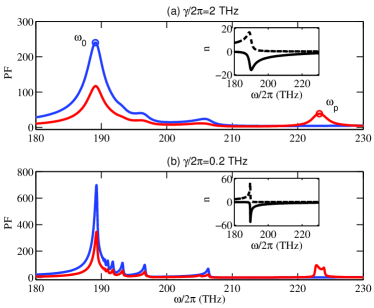
Figure 4: Purcell factor as a function of frequency for $\gamma/2\pi=2\,\mathrm{THz}$ (a) and $\gamma/2\pi=0.2\,\mathrm{THz}$ (b). The dot is located at $z_{0}=h/10=28\,$nm ($0.02\,\lambda_{0}$) above the NIM slab. The blue curves correspond to a $z-$polarized dipole, and the red curves correspond to an $x/y-$polarized dipole. The inset is the refractive index, $n$, vs frequency, where the dashed line corresponds to the imaginary part and the solid line to the real part (which is negative throughout the entire frequency range shown).

The PF (Eq. 17) is enhanced at the frequency of $\omega/2\pi\approx 189\,\mathrm{THz}\,(\approx\omega_{0}/2\pi)$, and the enhancement for a $z-$polarized dipole is larger than that for an $x$ or $y-$polarized dipole; part of the reason that the PF is larger for the $z-$polarized dipole is that it couples to the TM modes, which are more strongly influenced by material losses (through $\mu$); we have verified that the TM and TE PFs approach one another as $\gamma\rightarrow 0$, and this trend can partly be seen by comparing the TE and TM PFs in Fig. 4a and Fig. 4b. In the presence of the larger loss ($\gamma/2\pi=2$ THz) the peak $F_{z}$ (TM PF) is about 240 and the peak $F_{x/y}$ is about 120. When $\gamma/2\pi$ is decreased to 0.2 THz, the PF increases significantly to $\Gamma_{z}=720$ and $\Gamma_{x/y}=350$. The physical origin of these large PF enhancements comes from the slow energy velocities of the propagation modes. This can be seen from the dispersion curves (Fig. 2 and Fig. 3), where upon close inspection, we realize that we are obtaining the odd mode resonances, as is expected from dipoles near the surface where the local field is larger near the NIM surface; for example, the resonance around 207 THz corresponds to the $v_{g}\rightarrow 0$ region of the TE3 mode (cf.  Fig. 2(c) on the complex$-\omega$ band structure). In the complex$-\beta$ dispersion curves (Fig. 3(b)), this same resonance is seen as the point where the two branches of the TE3 mode split apart near 207 THz ($\beta\simeq 7\,\mu$m). The series of peaks below 200 THz and above $\omega_{0}$ are due to the slow group velocity region of the various odd modes, which approach one another at $\omega_{0}$.

In addition, we note that for the TE modes, there is a PF peak due to the plasmon resonance around 223 THz that has also been highlighted elsewhere, e.g. Refs. RuppinMartin2004 ; XuPRA2009 ; LiPEB2009 . What is particularly interesting, is that for reduced losses, this resonance splits into two (cf. Fig. 4(b)); moreover, by inspection of the band structure (cf. Fig. 3(b)), the lower-lying peak of this pair is actually due to the bound propagation modes (e.g., TE5), which is only visible in the complex$-\beta$ band structure. For larger losses, these individual peaks cannot be resolved, and one must then assume that the broadened peak near 223 THz for $\gamma/2\pi=2$ THz, is due to a combination of the TE SPP and bound modes contained within the light lines. We emphasize that this resonance, which is below the SPP frequency, is not observable with the complex$-\omega$ band structure, as discussed earlier; it is alo unique to the NIM structure.

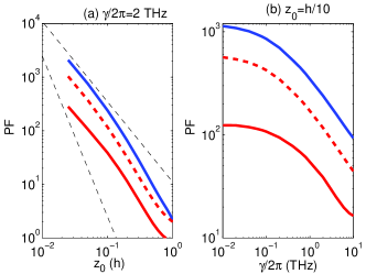
Figure 5: (a) The dependence of the maximum values in the PF on position $z_{0}$ for a loss factor of $\gamma/2\pi=2\,\mathrm{THz}$..  The solid blue and red curves correspond to the PF at $\omega_{0}$ for TM and TE modes respectively and the dashed red curve corresponds to the TE SPP mode. The upper and lower dashed grey curves show the scaling of $1/z_{0}^{1.5}$ and $1/z_{0}^{3}$, respectively. Even at the smallest distances from the NIM surface ($\sim 7\,$nm), the electrostatic limit (where a scaling of $1/z_{0}^{3}$ would occur) has still not been reached at the chosen frequencies (see text). (b) The maximum PFs as a function of damping factor for the dot located at $z_{0}=h/20$.  The curve labelling is the same as in (a). All curves are obtained at a fixed frequency.

Next, the PF for different dot positions $z_{0}$ is investigated. Similar to what happens near metal surfaces, as the dot is brought closer to the NIM slab surface, the PF will increase rapidly and formally diverge at the surface of the NIM slab. In fact, it is a straightforward exercise to show analytically that the electrostatic $\mathbf{G}$ at the surface of a half-space lossy structure has an imaginary part that diverges. One finds for the non-retarded terms (quasi-static approximation) MartinAO2001 : $\mathbf{G}(\mathbf{r}_{s},\mathbf{r}_{s})=\mathbf{G}^{0}(\mathbf{r}_{s},\mathbf{r}_{s})\mp\mathbf{G}^{0}(\mathbf{r}_{s},-\mathbf{r}_{s})(\varepsilon_{nim}-1)/(\varepsilon_{nim}+1)$, where the minus and plus sign refer to TE and TM polarization respectively, $\mathbf{G}^{0}$ is for free space, and $\varepsilon_{nim}$ is the permittivity of the NIM medium.  Because ${\rm Re}\left\{\mathbf{G}^{0}(\mathbf{r}_{s},\mathbf{r}_{s})\right\}$ diverges, any amount of loss in $\varepsilon_{nim}$, no matter how small, will lead to a divergent LDOS at the surface. Consequently, the quasi-static approximation will not work at the surface, and in general we should consider distances significantly larger than the emitter size if we are to employ the dipole approximation.

Figure 5(b) shows the dependence of the values of the PF at three different resconance peaks on the position $z_{0}$. Because of the expected LDOS divergence at the surface, we only show the behavior down to distances of $h/40$ ($z_{0}/\lambda_{0}=0.005$); we expect the dipole approximation to work to distances of around $h/10$ ($z_{0}/\lambda_{0}=0.02$). In obtaining these graphs we have fixed the frequency. The PF enhancements are found to decrease as a function of distance, as expected, but large values can still be obtained at distances ($\sim 0.4h$) or more.  For example, the TM peak has a PF of 10 at a distance of 100 nm from the surface. For metal surfaces, the TM SPP mode PF scales as $1/z_{0}^{3}$ for small distances (e.g. see Ref. JoulainPRB2003 ), which we have also verified for our structure (see Fig. 5(a)). This behavior is due to the electrostatic scaling of the evanescent contribution from the SPP, and for our structure, this scaling dominates for distances of around $z_{0}\leq 0.04\,h$. However, the scaling of the metamaterial modes is quite different: we obtain a scaling of around $1/z_{0}^{1.5}$ for the PF peak at $\omega_{0}$ and also for the TE SPP mode peak. In the limit of $\mu=1$, we again recover the $1/z_{0}^{3}$ scaling for these modes. Also in the case of the metamaterial, significant PFs can still be achieved for much larger distances away from the surface, even for $z_{0}=h$. The reason for this unexpected scaling is that the chosen resonance frequencies have not yet recovered the electrostatic limit, even for dipole distances as small as 7 nm from the surface; if we choose frequencies away from the waveguide peaks, then we indeed get the the $1/z_{0}^{3}$ scaling from the NIM, as expected.

The dependence of spontaneous emission on the damping factor is plotted in Fig. 5(b), which shows that increasing the damping factor decreases the peak spontaneous emission rate, while increasing the full width at half maximum (FWHM) of the PF resonance. However, even in the presence of very large losses (e.g., $\gamma/2\pi=$10 THz), we see that large PFs are still achievable. As expected, clearly there is also a large improvement in the PF enhancement if the nominal losses can be improved by an order of magnitude.

V.2 Lamb shift and far-field spectrum of spontaneous emission

The Lamb shift is another fundamental quantum effect whereby the vacuum interaction with a photon emitter can cause a frequency shift of the emitter lamb . Cavity QED level shifts of atoms near a metallic surface have been shown to be significant as one approaches the surface SipePRA1985 . For optimal coupling, usually these are studied at high frequencies (e.g., $\hbar\omega>4\,$eV), so as to couple to the TM SPP resonance; as a function of frequency, the level shift changes sign as we cross the resonance SipePRA1985 . For lower frequencxies, a $1/z_{0}^{3}$ van der Waals scaling again occurs Hinds1991 . Given the complicated modal structures of NIM waveguides, it is not clear what the Lamb shifts will look like, and to the best of our knowledge, Lamb shifts have never been studied in the context of metamaterial waveguides.

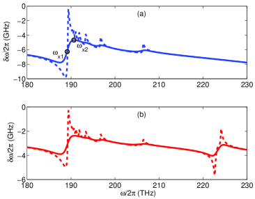
Figure 6: Frequency shift due to the inhomogeneous scattering when $\gamma/2\pi=2\,\mathrm{THz}$ (solid curves) and $\gamma/2\pi=0.2\,\mathrm{\ THz}$ (dashed curves). The dipole strength is $d=50\,D$ (see text). (a) The dot polarization is perpendicular to the slab surface (TM). (b) The dot polarization is parallel to the slab surface (TE).

The QED frequency shift of the emitter can be directly calculated via the real part of the scattered GF (Eq. (19)). Experimental dipole moments for semiconductor quantum dots vary from around $30\,\mathrm{D}$ (D=Debye) to $100\,$D silverman ; stievater , so here we adopt a realistic dipole moment of $d=50\,$D. The results for $z-$polarization and $x/y-$polarization are shown in Fig. 6(a) and Fig. 6(b), respectively. Our calculations indicate that the frequency for a dipole above the NIM slab will be significantly red-shifted relative to vacuum, with rich frequency oscillations as one sweeps through the NIM waveguide resonances. The Lamb shift at the $\omega_{0}$ resonance frequency for different loss factors $\gamma$ are identical, and are not zero; the nonzero shift at the main resonant frequency $\omega_{0}$ is due to the asymmetry of the PF, namely the series of waveguide resonances at the higher frequency end of $\omega_{0}$. The frequency shift at $\omega_{0}$ for TM modes is 6.3 GHz, and for TE modes is 3.5 GHz, and the difference between them mainly comes from TM SPP modes at $\omega_{pe}/\sqrt{2}\approx 490\,$THz. When the loss is reduced, the various modal contributions become more pronounced. It is worth highlighting that this frequency shift, which is completely unoptimized, is already comparable to some of the largest shifts reported for the real-index photonic crystal environment, e.g., $|\delta\omega|/\omega=4\times 10^{-5}$wang . In normalized units, we obtain frequency shifts around $|\delta\omega|/\omega=5\times 10^{-5}$, over a wide frequency range. This ratio is even larger for smaller distances (and larger dipole moments), however one must watch that the dipole approximation does not breakdown.

We also remark that these NIM Lamb shift features are substantially different to those predicted in typical metals. For example, we have calculated the Lamb shift from a half space of Aluminium and find that the Lamb shift in the same optical frequency regime is only -0.1 GHz, for an identical dipole and position.  Although closer to the SPP resonance (which is at 2780 THz), much larger values ($PF=322$ at $z_{0}=7\,$nm) can be achieved, the frequency dependence is relatively featureless, in contrast to that shown in Fig. 6 and the spontaneous emission is very strongly quenched in metals near the SSP resonance.

Finally, we turn our attention to the spontaneous emission radiation that can actually be measured. In the following, we use Eq. (21) to investigate the emitted spontaneous emission spectrum for two different exciton frequencies, $\omega_{d}=\omega_{d1}$ and $\omega_{d2}$ which are indicated in Fig. 6(a). The polarization of the quantum dot exciton is assumed to be along $z$, and the loss factor is $\gamma/2\pi=2\,$THz. The frequency dependence of the emitted radiation is shown in Fig. 7 for the two different dot frequencies. For $\omega_{d}=\omega_{d1}$, the shift at peak emissions is $-6.3\,$GHz and the enhancement in spontaneous emission rate is 240. For $\omega_{d}=\omega_{d2}$, the shift is $-4.7\,$GHz and the enhancement in the spontaneous emission rate is 135. Usually, with a large dipole moment of $d=50$ D and a spontaneous emission enhancement on the order of $100$, the the photon-dot interaction will enter the strong coupling regime and the emitted spectrum will show a typical spectral doublet.  However, since the emitted field away from the NIM is predominantly carried away by radiation modes, there the far field contains signatures of the QD coupling, even to near fields; however, because there is quenching in the far-field emission, strong coupling is not observable in the far field from the NIM waveguide-such effects could possibly be observed in the near field given suitable detection capabilities, e.g., from a scanning near field optical microscope. These features depend upon the properties of the GF propagator appearing the spontaneous emission formula (Eq. (21)). Comparing with the free space emission spectrum, the integrated emission in Fig. 7(a) and Fig. 7(b) is $1.8\times 10^{-4}$ and $1.6\times 10^{-3}$, respectively. Thus, the predicted far field spectra, which obtain Purcell factor and Lamb shift signatures, should certainly be observable experimentally.

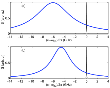
Figure 7: Detected spontaneous emission spectrum from a dot above the metamaterial (thick blue curve), compared with the emission from the same dot in free space (thin black curve). The dot location is $z_{0}=28\,$nm above the surface and the detector position is $2\lambda_{0}\approx 2800\,$nm above the quantum dot. The dot polarization is perpendicular to the slab surface. (a) The excition frequency is is $\omega_{d1}=189.1\,$THz. (b) The excition frequency is $\omega_{d2}=190.7\,$THz.

VI Conclusion

In summary, we have employed a rigorous medium-dependent theory and a stratified Green function technique, to investigate the enhanced emission characteristics of a single photon emitter near the surface of the NIM slab waveguide in the optical frequency regime. The origin of the predicted Purcell factor peaks is primarily due to slow light propagation modes which have been analyzed by calculating the complex band structure of this waveguide. Correspondingly, we also predict a significant frequency (Lamb) shift of the single photon emitter, with rich features that stem from the waveguide mode characteristics. All of our predictions are based on a realistic metamaterial model that includes both material dispersion and loss and scales to any region of the electromagnetic spectrum; the role of material loss and dipole position has also been investigated in detail. It is further shown that the rich emission characteristics at the surface can act as a sensitive and non-perturbative probe of below-light-line waveguide mode characteristics. These predicted medium-dependent QED effects are fundamentally interesting and may find use for applications in quantum information science.

This work was supported by the National Sciences and Engineering Research Council of Canada and the Canadian Foundation for Innovation. We thank O. J. F. Martin and M. Wubs for useful discussions.

References

- (1) V. G. Veselago, Sov. Phys. Usp. 10, 509 (1968).
- (2) J. B. Pendry, Phys. Rev. Lett. 85, 3966 (2000).
- (3) J. B. Pendry, D. Schurig, and D. R. Smith, Science 312, 1780 (2006).
- (4) K. L. Tsakmakidis, A. D. Boardman, and O. Hess, Nature 450, 397 (2007).
- (5) D. Schurig, J. J. Mock, B. J. Justice, S. A. Cummer, J. B. Pendry, A. F. Starr, and D. R. Smith, Science 314, 977 (2006).
- (6) G. Dolling, C. Enkrich, M. Wegener, C. M. Soukoulis, and S.Linden, Science 312, 892 (2006).
- (7) J. Valentine, S. Zhang, T. Zentgraf, E. Ulin-Avila, D. A. Genov, G. Barta, and X. Zhang, Nature 455, 376 (2008).
- (8) E. M. Purcell, Phys. Rev. 69, 681 (1946).
- (9) see, e.g., J. McKeever, A. Boca, A. D. Boozer, R. Miller, J. R. Buck, A. Kuzmich, H. J. Kimble, Science 303, 1992 (2004).
- (10) J. Kästel and M. Fleischhauer, Phys. Rev. A 71, 011804(R) (2005).
- (11) M. I. Stockman, Phys. Rev. Lett. 98, 177404 (2007).
- (12) D. R. Smith, D. Schurig, M. Rosenbluth, and S. Schultz, S. A. Ramakrishna and J. B. Pendry, Appl. Phys. Lett. 82, 1506(2003).
- (13) P. Yao, Z. Liang, and X. Jiang, Appl. Phys. Lett. 92, 031111 (2008).
- (14) A. Reza, M.M. Dignam, and S. Hughes, Nature 455, E10 (2008).
- (15) A. Sambale, S. Y. Buhmann, D-G Welsch, H. T. Dung, Phys. Rev. A 78, 053828 (2008).
- (16) J. Xu, N. Liu, and S. Zhu, Phys. Rev. E 73, 016604 (2006).
- (17) J. Xu, Y. Yang, H. Chen, and S. Zhu, Phys. Rev. A 76, 063813 (2007).
- (18) J. M. Wylie and J. E. Sipe Phys. Rev. A 30, 1185 - 1193 (1984)
- (19) J.M. Wylie and J.E. Sipe, Phys Rev A. bf 32, 2030 (1985).
- (20) K. Joulain, R. Carminati, J. P. Mulet, J.J. Greffet, Phys. Rev. B 68, 245405 (2003).
- (21) G. Sun, J. B. Khurgin, and R. A. Soref, Appl. Phys. Lett 90, 111107 (2007).
- (22) R. Ruppin and O. J. F. Martin, J. Chem. Phys. 121, 11358 (2004). We note that Eq. (1) should have replaced by in this paper, and as defined is .
- (23) J. P. Xu, Y-P Yang, Q. Lin, and S-Y Zhu, Phys. Rev. A 79, 043812 (2009).
- (24) J. Zhou, Th. Koschny and C. M. Soukoulis, Opt. Exp. 16, 11147-11152(2008).
- (25) G. Dolling, M. Wegener, C. M. Soukoulis and S. Linden, Opt. Lett. 32, 53-55 (2007).
- (26) P. Tassin, L. Zhang, T. Koschny, E. N. Economou, and C. M. Soukoulis, Phys. Rev. Lett. 102, 053901 (2009).
- (27) G.X Li, J. Evers, and C.H. Keitel, Phys. Rev. B 80, 045102 (2009).
- (28) M. Paulus, P. Gay-Balmaz, and O. J. F. Martin, Phys. Rev. E 62, 5797 (2000).
- (29) A. Taflove and S. C. Hagness, Computational Electrodynamics: The Finite-Difference Time-Domain Method, 3rd ed. Norwood, MA: Artech House, 2005.
- (30) A.W.Synder and J.D.Love, “Optical Waveguide Theory,” (Chapman&Hall, London,1983)
- (31) I.V.Shadrivov, A.A.Sukhorukov, Y.S.Kivshar, Phys.Rev.E 67, 057602 (2003).
- (32) T.J.Cui, J.A.Kong, Phys.Rev.B 70, 205106 (2004).
- (33) H. T. Dung, S. Y. Buhmann, L. Kno, D-G Welsch, S. Scheel, and J. Kästel, Phys. Rev. A 68, 043816 (2003).
- (34) H. T. Dung, S Scheel, D-G Welsch, and L Knöll, J. Opt. B 4, 169 (2002).
- (35) H. T. Dung, L. Knöll, and D-G Welsch, Phys. Rev. A 62, 053804 (2000).
- (36) W. P. Healy Phys. Rev. A 22, 2891 (1980)
- (37) E. A. Power and T. Thirunamachandran Phys. Rev. A 25, 2473 (1982)
- (38) M. Wubs, L. G. Suttorp, and A. Lagendijk, Phys. Rev. A 70, 053823 (2004).
- (39) S. Hughes and P. Yao, Opt. Exp. 17, 3322 (2009).
- (40) H. T. Dung, S.T. Buhmann, L. Knöll, D-G Welsch, S. Scheel, and J. Kästel, Phys. Rev. A 68, 043816 (2000).
- (41) see, e.g., H.A. Bethe, Phys. Rev. 72, 339 (1947).
- (42) P. De Vries, D. V. van Coevordenm, and A. Lagendijk, Rev. Modern Phys. 70, 447 (1998).
- (43) S. Scheel, L. Knöll, and D.-G. Welsch, Phys. Rev. A 60, 4094 (1999).
- (44) P. W. Milonni, The Quantum Vacuum (Academic, San Diego, 1994).
- (45) T. Ochiai, J-I. Inoue, and K. Sakoda, Phys. Rev. A 74, 063818 (2006).
- (46) S. A. Ramakrishna and O. J. F. Martin, Opt. Lett. 30, 2626 (2005).
- (47) M. S. Tomaš, Phys. Rev. A 51, 2545 (1995).
- (48) P. Sheng ,Introduction to wave scattering, localization, and mesoscopic phenomena, Academic Press, 1995.
- (49) V. S. C. Manga Rao and S. Hughes, Phys. Rev. B 75, 205437 (2007); see also G. Lecamp, P. Lalanne, and J.P. Hugonin, Phys. Rev. Lett. 99, 023902 (2007).
- (50) T. Lund-Hansen, S. Stobbe, B. Julsgaard, H. N. Thyrrestrup, T. Sünner, M. Kamp, A. Forchel, and P. Lodahl, Phys. Rev. Lett. 101, 113903 (2008)
- (51) K. L. Silverman, R. P. Mirin,S. T. Cundiff, and A. G. Norman, Appl. Phys. Lett. 82, 4552 (2003)
- (52) T. H. Stievater, Xiaoqin Li, D. G. Steel, D. Gammon, D. S. Katzer, D. Park, C. Piermarocchi and L. Sham, Phys. Rev. Lett. 87, 133603 (2001),
- (53) X. Wang, Y. S. Kivshar and B. Gu, Phys. Rev. Lett. 93, 073901 (2004).
- (54) P. Gay-Balmaz and O.J.F. Martin, Applied Optics 40, 4562 (2001).
- (55) E. A. Hinds and V. Sandoghdar, Phys Rev. A. 43, 398 (1991).