Undulatory Locomotion

Abstract

Undulatory locomotion is a means of self-propulsion that relies on the generation and propagation of waves along a body. As a mode of locomotion it is primitive and relatively simple, yet can be remarkably robust. No wonder then, that it is so prevalent across a range of biological scales from motile bacteria to gigantic prehistoric snakes. Key to understanding undulatory locomotion is the body’s interplay with the physical environment, which the swimmer or crawler will exploit to generate propulsion, and in some cases, even to generate the underlying undulations. This review focuses by and large on undulators in the low Reynolds numbers regime, where the physics of the environment can be much more tractable. We review some key concepts and theoretical advances, as well as simulation tools and results applied to selected examples of biological swimmers. In particular, we extend the discussion to some simple cases of locomotion in non-Newtonian media as well as to small animals, in which the nervous system, motor control, body properties and the environment must all be considered to understand how undulations are generated and modulated. To conclude, we review recent progress in microrobotic undulators that may one day become commonplace in applications ranging from toxic waste disposal to minimally invasive surgery.

I The universality of undulatory locomotion

One of the crucial existential requirements of microbial and animal life is movement. Whether for foraging, for mating or to avoid danger, most non-plant life forms have evolved mechanisms of locomotion, and the solutions are diverse. Microorganisms are too small to have many components in their motor system. Larger terrestrial animals may resort to limbs that support the weight of the animal and thus deal with gravitational forces. Other animals have adopted a variety of forms that keep them close to the ground or even underground, minimizing the effects of gravity. One example is the sandfish (small lizards with smooth scales), whose undulations effectively fluidize the surrounding sand and allow it to swim through the granular flow Baumgartner et al. (2008). Marine, subterrainean and flying species have to contend with very different physical environments. And yet, all of locomotion can probably be divided into a small number of fundamental classes. Of these, undulatory locomotion that relies on wave propagation along the body, is remarkably widespread.

No wonder. To undulate, a system does not require limbs, only a body. Even single celled microorganisms use elastic filaments that extend from the cell membrane, or modulate the body shape, to undulate. Paramecia, like many single celled eukaryotic organisms (protozoa), are covered with cilia that are used much like little oars to synchronously row through water. Motile bacteria use one or more long helical filaments, called flagella, that extend from the cell membrane and act as a propeller. These flagellated bacteria swim by rotating all their helical flagella one way, while the cell body rotates in the opposite direction. E. coli, for example uses such a mechanism to swim at 35 diameters per second Berg (2000, 2004). Some motile unflagellated bacteria resort instead to the propagation of low amplitude waves on the surface of their bodies Stone and Samuel (1996); Ehlers et al. (1996).

In the animal kingdom, limbs might come in handy for some purposes, but when they are more of an impediment, swimmers can choose to press them against the body or use them to complement the undulations. Crawlers may need to burrow into narrow nooks. And many species may exploit the flexibility and adaptability of crawling like gaits to allow them to move through a variety of different physical environments (such as eels, that not only swim but are also capable of burrowing through sand or mud Breder (1926)). Thus, it is not surprising to find undulations as the primary means of locomotion in a variety of larvae, worms, lizards, snakes, fish, and even some mammals ranging in size from tiny microbes to the monster (13m long) prehistoric titanoboa snakes Head et al. (2009).

Animals use a variety of different forms of undulation to locomote. These can crudely be classified into horizontal or vertical, direct (in the direction of motion) or retrograde (opposite the direction of motion) and longitudinal or transverse. Fish usually flap their bodies from side to side, whereas whales and other marine mammals undulate up and down. Typically, to move in a given direction, retrograde waves are required, that propagate opposite to the direction of motion (i.e., from head to tail to achieve forward motion). In other words, if the body wave travels backward, the environment applies forward forces. But Biology is full of exceptions. Some annelids, including the polychaete worm Nereis virens La Spina et al. (2007), as well as several protozoa, such as the motile alga Ochromonas malhamensis Jahn et al. (1964) exhibit the remarkable property that the organism moves in the same direction as the wave propagation. To understand how such a counter-intuitive mode of locomotion can be achieved, one must first notice a key similarity between the body of Nereis and the flagella of Ochromonas. In both cases, the body/flagellum is lined with ‘bristles’ which jut out at right angles to the long axis. These protrusions act much like oars, generating significant drag forces when the body is moved forwards or backwards, but having minimal effect when it is moved sideways. In contrast, conventional (retrodgrade) undulations rely on stronger resistance to sideways motion.

If there is a unifying principle to all of the above, it is that undulating motion is typically constrained by frictional or drag forces of the environment, rather than by gravitational forces. For instance, most swimmers can float in water using buoyancy, but self-propulsion becomes much more energy intensive than in air or on the ground. This is all the more severe in turbulent waters or when swimming upstream in a river. Fish use a range of individual and group strategies to exploit the hydrodynamics and minimize energy expenditure. Many fish, for example, can minimize power expenditure (i.e., muscle work) by recycling energy from vortices in turbulent flows. In fact, by swimming in schools, trout kinematics are not so different from that of passive hydrofoils (mimicking flag waving motion) Müller (2003); Liao et al. (2003); Liao (2007). Terrestrial crawlers (and swimmers Baumgartner et al. (2008); Maladen et al. (2009)) keep close to the ground, so they are much more constrained by the terrain and its associated frictional forces than by gravity. But this is perhaps most obvious in the so called low Reynolds number regime, where inertial forces become altogether negligible. In all of the above, the immediate implication is that undulatory locomotion arises from the interaction between the dynamics of the body and the physics of the environment and hence places strong constraints on the shape of the body.

II Theory

In this paper, we will try to restrict ourselves to some of the simplest cases of undulatory locomotion operating in the low Reynolds number regime and where two dimensional treatments suffice; body shapes are long and slender, and the environment is relatively simple. We begin with an introduction to some of the theoretical foundations in fluid mechanics and their applications to self-propulsion in general and to undulatory locomotion in particular.

II.1 What is the Reynolds number?

Fluid mechanics has long been of interest to physicists. Already Isaac Newton postulated how fluids of different consistencies respond to forces. Perhaps, when Isaac Newton took a break from pondering the motion of falling apples, he was holding a spoon over his cup of afternoon tea, and dragging it along the surface. He would have noticed that the top layer of the fluid was dragged along. How much more difficult would this be if he had done the same across a jug of honey? Newton postulated that the force required to keep a flat spoon moving at constant speed $v$ would follow

$$F\propto A\left.\frac{dv}{dy}\right|_{\text{moving spoon}}$$ (1)

where $A$ is the contact area of the spoon, and $v(y)$ is the speed profile of different slices of fluid as one moves a distance $y$ away from the spoon. The proportionality constant is called the viscosity of the fluid (or sometimes the dynamic or Newtonian viscosity) $\mu$. The gradient of the velocity profile $dv/dy$ reflects the strength of the dragging and indicates how nearby slices of fluid are differentially dragged . In fact, not all fluids obey the linearity of Eq. (1), but those that do are called Newtonian fluids. Examples include air, water and indeed honey with respective viscosities of $O(10^{-5})$Pa$\cdot$s, $O(10^{-3})$Pa$\cdot$s and $O(10^{4})$Pa$\cdot$s.

Now if we change the speed with which we are moving the spoon (or stop it altogether), we must also consider the inertia of the fluid. Inertial effects will dominate over viscous forces when the spoon is sufficiently fast, or alternatively, when the fluid has sufficiently low viscosity. In this case, the force applied by the spoon on the fluid can result in nonlinear convective and turbulent flows, which will then feed back and influence the motion. Let us try to determine when such inertial effects are important.

To do so, consider the motion of an object through a Newtonian fluid. Suppose the velocity $v$ of the fluid drops off linearly away from the object. The viscous forces in the fluid around the object are given by $\mu Adv/dy$, which will then scale as $O(\mu\ell^{2}v/\ell)=O(\mu\ell v)$, where $\ell$ is a characteristic size of the object. The inertial forces (due to the fluid’s momentum in the same region $mdv/dt$) should scale as $O(\rho\ell^{2}v^{2})$ where $\rho$ is the density of the fluid. The ratio of these two expressions is then characterized by a single dimensionless scaling parameter

$$\text{Re}=\frac{\rho\ell^{2}v^{2}}{\mu\ell v}=\frac{\rho\ell v}{\mu}\;,$$ (2)

where Re is the conventional shorthand for the ‘Reynolds number’. When $\text{Re}\gg 1$ inertial forces dominate. By contrast, if $\text{Re}\lessapprox 1$ the viscous forces dominate the flow and the fluid largely responds to external forces in a passive manner. To give ballpark figures, a person swimming in water might experience a Reynolds number of $O(10^{4})$. If we tried to swim through honey, we might feel a Re around $O(10^{-3})$ and bacteria swimming in water may feel Reynolds numbers as low as $O(10^{-5}$)!

The Reynolds number can also be obtained from the governing equation in fluid dynamics, the so-called Navier-Stokes equation (given here in simpler form for incompressible fluids, i.e., $\nabla\cdot v=0$)

$$-\nabla p+\mu\nabla^{2}v=\rho\frac{\partial v}{\partial t}+\rho(v\cdot\nabla)v\;.$$ (3)

Here, the left hand side describes pressure and viscous terms, and the right hand side describes inertial terms, which vanish at low Re . In fact, it is easy to see here, that for an object with a characteristic length $\ell$, we can recover the Reynolds number as the ratio of the inertial term $\rho(v\cdot\nabla)v$ to the viscous drag term $\mu\nabla^{2}v$. In most of what follows, we will need only the low Re reduction of the Navier-Stokes equation

$$\mu\nabla^{2}v=\nabla p\;.$$ (4)

II.2 Self-propulsion in low Re environments and the scallop theorem

Most of our intuition comes from our day to day experiences of the high Re world in which inertia must be overcome. When you start off in your car, a torque is applied to the wheels, which in turn apply a backwards directed force to the surface of the road. The reactive (forwards directed) frictional force on the car gives rise to acceleration. At some speed this propulsive force is counter-balanced by wind resistance and the velocity settles. The elimination of inertia at low Re means that any nonzero resultant force acting on an object will give rise to infinite acceleration. Thus, somewhat counterintuitively, the total net force and torque acting on an object moving in a low Re environment will at all times be zero. As an example, suppose a small swimmer is moving at constant velocity, and then stops swimming. The above condition will result in immediate deceleration and the swimmer will stop. Swimming is indeed hard work at low Reynolds numbers. Curiously, low Reynolds number physics is remarkably reminiscent of the Aristotelian view of physics, in which objects will remain stationary in the absence of external forces. Aristotle’s mechanics has long been dismissed as fundamentally flawed and superceded by Newtonian mechanics, so it is reassuring to see that this theory too has found its natural place.

Let us now consider a small swimmer (and hence at low Re). To have any chance of moving, it must be able to change its shape. The sum of all internal forces must clearly be zero (for the same reason you cannot lift yourself up by your boot straps). The change of shape will result in some motion of parts of the body in a global coordinate frame, which will then elicit reactive drag forces. But since these reactive forces must sum to zero, the organism as a whole will move in such a way that this is the case. This condition is sufficient to uniquely determine the motion of the whole organism given a known time series of body configurations and known environmental properties.

In fact the low Re physics imposes constraints on the possible shape changes that will result in progress. This was realized by Ludwig Ludwig (1930) and then by Purcell Purcell (1977) who nicely formulated it as the scallop theorem. Consider a scallop that opens and closes its shell in water to move. At sufficiently high Re, the slow opening and rapid shutting of the shell pushes water out and propels the scallop in the opposite direction. At low Reynolds number, the flow of water into and out of the scallop over one cycle would be the same, regardless of the speed. Scallops would make no net progress at low Re.

The derivation of this theorem is straightforward and instructive. We begin with the Navier-Stokes equation at low Reynolds number [Eq. (4)]. Note that this equation is time independent. This means that speed makes no difference to the motion. Only the sequence of configurations of the body determines the motion. But if that sequence is time reversible, such that moving forward or backward in time involves the same sequence of shapes, then no overall progress can result.

How then is propulsion achieved at low Re? It is reasonable to assume that successful propulsion always relies on a repetitive “stride” or cyclical motion, but can we move beyond the no-go scallop theorem towards a unifying theory of shape changes that sustain self-propulsion at low Re?

II.2.1 A generalized scallop theorem

Consider some cyclic motion of a low Reynolds number swimmer in a Newtonian fluid. Following Shapere and Wilczek Shapere and Wilczek (1989) we could construct an alphabet of all possible shapes $\{S_{0}\}$ of the swimmer, all at the same location and orientation (the origin). Then the motion of a deformable body undergoing an ordered sequence of body-shape changes $S_{0}(t)$ will be described by a rotation and displacement of the body to its appropriate orientation and location $S(t)$ via

$$S(t)=\mathcal{R}(t)S_{0}(t)\;,$$

where $\mathcal{R}$ combines both rotation and displacement operations. Now to follow shape changes in continuous time we would like to follow infinitessimal shape changes, and hence it is convenient to introduce an exponential form (so infinitessimal generators will form a Lie algebra). In particular, defining

$$\frac{d\mathcal{R}}{dt}=\mathcal{R}\left(\mathcal{R}^{-1}\frac{d\mathcal{R}}{dt}\right)\equiv\mathcal{R}A$$

allows us to write

$$\mathcal{R}(t)=\bar{P}\exp\left({\int_{0}^{t}A(t^{\prime})dt^{\prime}}\right)\;,$$ (5)

where $\bar{P}$ represents ordering terms in the expansion of the exponent with later terms to the right . Although $A(t)$ is in general time dependent, the linearity of the Navier-Stokes equation at low Re means that speed does not matter. Indeed, as we have already argued, in the absence of inertial effects, the sequence of shape changes completely specified the rotation and displacement of a body. Thus, $A(t)$ may be recast in an effectively time-independent geometric manner Shapere and Wilczek (1989). Define a vector over shape space, also denoted $A$, whose projection onto the “direction” (in shape space) $dS_{0}/dt$ is just $A(t)$, via

$$A(t)\equiv A_{\dot{S}_{0}}[S_{0}(t)]\;.$$

Thus, at low Re, an integral over time can be recast as an integral over shapes and Eq. (5) becomes

$$\mathcal{R}(t)=\bar{P}\exp\left({\int_{S_{0}(0)}^{S_{0}(t)}A[S_{0}]\cdot dS_{0}}\right)\;.$$

For a cyclic stroke, the net rotation and displacement are then

$$\mathcal{R}(t)=\bar{P}\exp\left({\oint A[S_{0}]\cdot dS_{0}}\right)\;.$$

Thus, the net progress our swimmer makes in each cycle is proportional to the area circumscribed in shape space. For a simple back-and-forth motion such as the scallop’s, no area is “cut out” and so no overall progress can be made. This geometric formulation therefore generalizes Purcell’s scallop theorem by relating the progress of a low Re swimmer to a geometric phase (akin to a classical Berry’s phase). Of course, to determine how much progress is actually made still requires solving the fluid dynamic equations to obtain the shape space vector $A[S_{0}]$. This generalized formulation of the scallop theorem is due to Shapere and Wilczek Shapere and Wilczek (1989).

II.2.2 Spherical symmetry breaking for propulsion

While violating the time reversibility condition of the scallop theorem is necessary for successful propulsion at low Re, there is one other asymmetry that needs mentioning. Regardless of scale or Reynolds number, successful propulsion requires an asymmetry or anisotropy in the environmental resistance to the motion of the body. Consider a compact shape that undergoes a time-asymmetric cycle of shape changes, but remains at all times spherically symmetrical. It is trivial to see that such a shape would go nowhere. Thus, some form of spherical symmetry breaking is needed to achieve locomotion.

Indeed, nearly all life forms, from bacteria to mammals have a distinct body axis or polarity, which dictates the direction of motion. When an elongated body is moving forwards (parallel to its long axis) at low Re, it will displace less fluid per unit time than when moving sideways (normal to its long axis). Thus, it will encounter a smaller resistance from the fluid. The ability of a deformable body to modulate the level of resistance it encounters in different directions allows, in principle, for motion to be possible. This point will be revisited in Sec. II.3.1.

To demonstrate the minimal conditions for swimming, we give two very simple examples: one of a generalized scallop that can rotate, but cannot swim (or propel itself in one direction), and another of a minimal swimmer. Consider a cyclical version of Purcell’s scallop, where instead of opening and shutting, the scallop’s opening angle keeps increasing (at $2\pi$ per cycle). Shapere and Wilczek Shapere and Wilczek (1989) already noted that the Scallop theorem assumes that the scallop cannot turn through more than $2\pi$ on its hinge). However, if we allow the scallop to do so, and assuming the two arms are even, the scallop will still get nowhere. To break time reversal symmetry, one arm could be longer than the other, and hence subject to a greater resistive drag force, as shown in Fig. 1A. In this case, the scallop can rotate, but will not achieve any lasting translation (Fig. 1B).

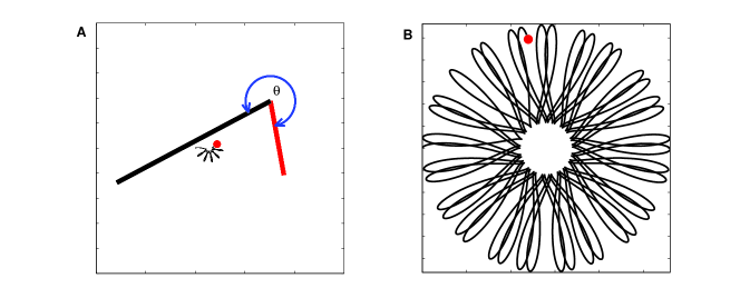
Figure 1: A. A variation on Purcell’s scallop in which the two arms have different lengths and are allowed to rotate freely around (like a wheel). Arms are modeled as slender cylindrical bodies. The medium is modeled as Newtonian ($K$ = 2). The path of the scallop’s “center of mass” (CoM, red dot) is shown in black. After a few rotations, the CoM appears to undergo both translation and rotation. However, the CoM never leaves a circular area of small radius, as can be seen by following the trajectory over sufficiently many cycles (B). Each ‘petal’ corresponds to one cycle of rotation through $2\pi$.

Consider, by contrast, the following push-me-pull-you example due to Avron et al. Avron et al. (2005) in Fig. 2. Here we have two perfectly spherical shapes that are experiencing isotropic drag at all times. However, by allowing the spheres to inflate and deflate, the relative drag forces they experience change in time, allowing the motion of the spheres to be asymmetrical as well. In either case, applying Shapere’s and Wilczek’s formalism above should demonstrate that an area is indeed carved out in shape space, leading, in the asymmetric scallop case, to an overall rotation and, in the push-me-pull-you case, to an overall displacement. (Note that the push-me-pull-you example involves two degrees of freedom, but some restricted forms of propulsion can also be achieved with only a single degree of freedom.)

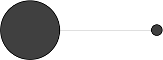
Figure 2: Schematic of a self-propelled push-me-pull-you device, adapted from Ref. [Avron et al., 2005]. To move, the device follows a cyclical sequence of steps that include: (i) shortening the connecting rod between the spheres; (ii) inflating and deflating the two spheres so their volumes are switched; (iii) lengthening the rod to its original length; and (iv) deflating and inflating the two spheres to their original sizes. For the initial conditions depicted here, this sequence will lead to motion to the left.

II.3 Incompressible fluid dynamics at low Re

To solve the equations of motion of a body moving through a fluid is a daunting task which, in general, requires a solution to the Navier-Stokes equations. When convective and turbulent forces dominate, this is indeed arduous , but even at low Reynolds numbers the problem is rarely solved analytically. Below, we introduce the basic equations for relatively simple but limited classes of problems. We begin with the condition for incompressible fluids $\nabla\cdot v=0$. Taking the curl of Eq. (4) yields

$$\nabla^{2}(\nabla\times v)=0\;.$$ (6)

To solve the equation for swimmers in a fluid, we need only add boundary conditions, satisfied by the fluid at the boundary of the swimmer’s body. This is typically the no-slip condition

$$v|_{S}=\frac{\delta S}{\delta t}\;,$$ (7)

which requires that the fluid is perfectly dragged along at the boundary $S$.

We now consider two simplifications of the Navier-Stokes equation for an incompressible fluid at low Re [Eq. (4)]. First, if the velocity profile $v$ takes the form of a so-called potential flow $v=\nabla\phi$, with $\nabla^{2}\phi=0$, then Eq. (6) is automatically satisfied. In this case, solving the Laplace equation for a scalar field presents a vast simplification over the Navier-Stokes equation. For example, this approach allows us to prove Stokes’ Law, namely, that the speed $v$ at which a sphere of radius $r$ will tend to be towed in a Newtonian fluid with viscosity $\mu$ under the application of a force $F$ is given, in the limit of small Re, by

$$F=6\pi\mu rv\;.$$ (8)

Importantly, this approach can also be used to derive the theory of slender bodies, which underlies most of our understanding of undulatory physics at low Re.

A more general simplification occurs in 2D. Then we may always write $v=(\partial U/\partial y,\,-\partial U/\partial x)$ where $U$ is a scalar potential. Hence Eq. (6) reduces to the biharmonic equation

$$\nabla^{4}U=0\;.$$ (9)

This, in addition to the no-slip condition, gives a full description of low Re (incompressible) fluid dynamics in 2D.

II.3.1 Slender body theory

Undulations are particularly appealing to study, not only because of their ubiquity but also because the motion can be elegantly formulated as the propagation of a wave. In particular, in low Re it turns out that some very general statements can be made within what is often dubbed slender body theory. We owe our understanding of the physics of undulatory locomotion in large part to the pioneering works of physicists and applied mathematicians (such as G. I. Taylor, M. J. Lighthill and G. J. Hancock) as well as zoologists (notably J. Gray, H. W. Lissmann and H. R. Wallace) in the 1950s Taylor (1951, 1952); Hancock (1953); Gray (1953); Wallace (1958, 1959, 1960). These authors described the locomotion, analyzed the physical forces and derived the mathematical framework that we still use today to understand low Re undulatory locomotion. (Incidentally, the theory developed for high Re undulations bears many similarities to slender body theory and is called elongated body theory Lighthill (1971)). In this section, we present a brief overview of key results for slender body locomotion.

As we introduced above, two key asymmetries are required for an organism to be capable of low Re swimming. Not only must the undulation be asymmetric under time reversal, but some asymmetry in the environmental resistance is also required (the latter being a more general requirement of locomotion at any Re). Organisms that use undulatory locomotion are generally long and thin; in fluids, this guarantees asymmetry in the resistance to forward (or backward) and sideways motion.

Now as already noted, analytically solving the motion of non-spherical shapes in a fluid is non-trivial. Slender body theory approaches this by deriving approximate solutions of the Navier-Stokes equation for no-slip boundary conditions applied to long cylindrical or similarly elongated shapes. These solutions take the form of force-velocity relations. Decomposing those into their vector components then leads to two different linear force-velocity relations along the major and minor axis of the object. It then becomes possible to write drag equations [analogous to Eq. (8)] as

$$F_{i}=-c_{i}\,v_{i}\;,$$ (10)

where $c_{i}$ are the effective drag coefficients for motion tangent ($c_{\parallel}$) and normal ($c_{\perp}$) to the local body surface.

Within this framework, R. G. Cox was able to derive equations approximating $c_{\parallel}$ and $c_{\perp}$ as functions of the length and radius of the body, and the viscosity of the Newtonian fluid Cox (1970). Approximating the body shape as a prolate ellipsoid, J. Lighthill obtained similar but slightly more accurate expressions for the effective drag coefficients Lighthill (1976):

$$c_{\perp} =L\,\frac{4\pi\mu}{\rm{ln}(2q/r)+0.5}$$

$$c_{\parallel} =L\,\frac{2\pi\mu}{\rm{ln}(2q/r)}\;,$$ (11)

where $L$ is the body length, $r$ is the body radius, $q=0.09\lambda$ (with $\lambda$ being the wavelength of the undulation) and $\mu$ is the viscosity of the fluid. The requirement of asymmetric drag forces can be neatly expressed in terms of the ratio $K=c_{\perp}/c_{\parallel}$ which must have a value other than unity if progress is to be possible. Notice that the viscosity of the fluid has no effect on this ratio. Rather, it is completely determined by the geometry of the object. For worm-like shapes, $K$ typically takes values around $1.5$, whereas for infinitely long cylinders, $K$ approaches 2 ($K\rightarrow 2$).

II.3.2 Undulations in rigid channels

To understand how propulsion is generated, we consider the simple case of a cylindrical organism whose body undulates sinusoidally in a plane. From the scallop theorem we know that a standing wave will be unable to propel the organism, so instead consider a traveling wave that is propagated backward from head to tail, and is therefore not time symmetric. In the absence of any fluid or walls (i.e., in vacuum), the body wave could still propagate backwards at velocity $v_{\rm{wave}}$, but the organism would remain stationary. By contrast, now consider the limit $K\rightarrow\infty$, which could be achieved by placing the organism in a tightly fitting sinusoidal channel with the same amplitude and wavelength as the body wave but with rigid walls Gray (1953). Within this channel, the wave is by definition stationary in global coordinates, forcing the organism forwards at a velocity $v_{\rm prog}=-v_{\rm wave}$.

Let us examine how propulsion is achieved down the channel. As the wave is propagated, the channel will apply a reactive force sufficient to prevent any motion in the normal direction. These reaction forces will only occur on the leading (i.e., backwards facing) edge of the wave. Now, the forwards directed components of these forces will add up, yielding a net propulsive force down the channel while any sideways directed components will cancel out. Hence, the organism will move forwards through the channel, with some velocity $v_{\rm prog}$. As the organism slides forwards, it will rub against the sides of the channel and evoke reactive drag forces. Again the sideways directed components will cancel out over a cycle, but the backwards directed components will sum, yielding a net retarding force opposite to the direction of motion. The propulsive force exerted by the walls of the channel will be exactly sufficient to counteract this retarding force when the organism progresses at velocity $v_{\rm prog}=-v_{\rm wave}$.

II.3.3 Low Re undulations: “slip” formulation

Clearly, the $K\rightarrow\infty$ case can be trivially solved without recourse to fluid dynamics or slender-body theory. Consider the same organism in a fluid, i.e., with finite $K$ (the same reasoning will apply for any $K>1$). Now, the normal component of velocity $v_{\perp}$ must be non-zero if the normal force $F_{\perp}$ is to be non-zero. So, rather than the wave remaining stationary in the global frame, it will slip backwards at some velocity $v_{\rm{slip}}$ (with $|v_{\rm{slip}}|\leq|v_{\rm{wave}}|$) while the organism moves forwards at velocity $v_{\rm prog}=-(v_{\rm wave}-v_{\rm slip})$ . This is schematically illustrated in Fig. 3A. An approximation of slender body theory can be obtained from the so called force resistivity theory and is due to Gray and Hancock Gray and Hancock (1955). Here, rather than solving the Navier-Stokes equations for a long and slender body, the forces are approximated independently at each point (using equations of the form $F_{i}=c_{i}\,v_{i}$ as before) and then integrated over the body length. Thus, any correlations in the fluid due to the spatially extended nature of the body are neglected. Applying this formalism to a perfectly sinusoidal body wave of low amplitude ($A$) and short wavelength ($\lambda\ll L$) (Fig. 4A), Gray et al. Gray and Hancock (1955); Gray and Lissmann (1964) were able to derive an expression relating $v_{\rm{slip}}$ to $v_{\rm{wave}}$:

$$v_{\rm{slip}}=v_{\rm{wave}}\frac{B+1}{KB+1}\;,$$ (12)

where $B=2\pi^{2}A^{2}/\lambda^{2}$.

In general, for a given locomotion waveform, the degree of slip depends only on $K$. Relating this back to the case of locomotion in a rigid channel where we effectively have $K\rightarrow\infty$, we can see that for any $B$, we will have $v_{\rm{slip}}\rightarrow 0$, so that over a single period of undulation the body travels a distance of one wavelength. Interestingly, slender body theory is valid for any $K>0$. For $K=1$ we obtain $100\%$ slip (equivalent to a vacuum, or completely isotropic environmental resistance) and for $K<1$ we observe direct wave propagation, with the body progressing in the same direction as the wave (Fig. 3B).

While approximate, the simplicity and tractability of the force resistivity theory has led to its extensive application in biological domains, in particular for the study of flagellar propulsion in viscous fluids and nematode locomotion in viscous and visco-elastic fluids (see below). In both cases, comparisons either against slender body theory Johnson and Brokaw (1979) or against data Berri et al. (2009) have concluded that the approximations are reasonable.

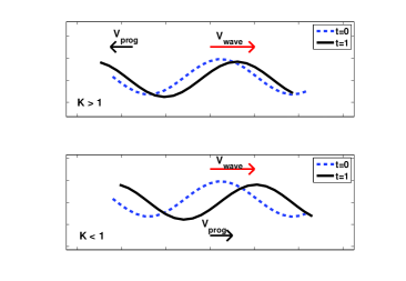
Figure 3: The effect of $K$ on propulsion. An undulating body propagates a sinusoidal wave to the right at velocity $v_{\rm wave}$ (red arrow). If $K=1$, no motion will result (not shown). If $K>1$, the body moves at velocity $v_{\rm prog}$ in the direction opposite to $v_{\rm wave}$, with $|v_{\rm prog}|\leq|v_{\rm wave}|$. If $K<1$, the situation reverses and the body moves in the same direction as $v_{\rm wave}$, with $v_{\rm prog}<v_{\rm wave}$.

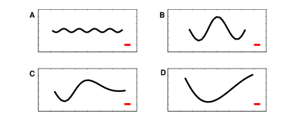
Figure 4: Assessing the validity of Eq. (12) with a physics simulator (see text for details). A. The analytic result of Gray et al. Gray and Lissmann (1964) is an excellent approximation for an undulator with a perfectly sinusoidal wave, a wavelength that is short relative to the body length and of a low amplitude. B. A purely sinusoidal idealization of the C. elegans crawling wave. The same equation handles such a wave reasonably well but with small errors due to the increased amplitude and wavelength. C. A more realistic C. elegans crawling waveform in which the wavelength increases towards the tail introduces significant errors. D. A realistic C. elegans swimming waveform in which the wavelength is greater than the body length is very poorly described by the analytic approximation.

II.3.4 Beyond Newtonian fluids

It is remarkable how adept biological organisms are at adapting to different environments and modulating their behavior. Many organisms exhibit enormous flexibility in navigating a wide range of environments, whether this involves changes of gait or continuous modulation of a single behavior. At the same time, there are conditions in which organisms display very uncoordinated locomotion or else fail to make progress altogether. These may correspond to environments that are not usually encountered in an organism’s natural habitat, or – more often in the geneticists’ laboratory – to mutants that lack an essential protein. The investigation of biological forms of undulatory locomotion across different physical environments dates back to the early 20^th century Looss (1911); Gray and Lissmann (1964); Wallace (1958, 1959, 1960) and is playing an increasingly important role in genetics and in neuroscience Horner and Jayne (2008); Lockery et al. (2008); Berri et al. (2009); Pierce-Shimomura et al. (2008).

Until now, we have limited ourselves to Newtonian fluids, which are fully described by the viscosity of the medium, but many low Re swimmers in fact move through complex fluids or other ‘soft’ environments. For slender bodies in a Newtonian fluid, the ratio of drag coefficients $K$ is fully determined by the geometry and cannot exceed 2. In contrast, in non-Newtonian environments, $K$ (if and when it is well defined) is both a function of the geometry and of the medium. Strictly speaking, viscosity is not defined in non-Newtonian fluids, since the linearity of Eq. (1) is violated. Thus even the Navier-Stokes equation is not applicable. For example, the fluid may have some non-trivial structure, it may have energy storage capacity (e.g., elasticity), or perhaps the properties of the fluid may depend on the speed with which it is deformed. Of these cases, visco-elastic fluids (and visco-elastic approximations of gels) are probably the most relevant to biological swimmers. Slender body or resistive force theories can both be straightforwardly extrapolated to model visco-elasticity when the elastic properties of the fluid can be approximated by effectively stronger resistive drag coefficients in the normal direction, thus increasing the ratio $K$ Gray and Lissmann (1964)^,. In what follows, we loosely call such extensions to Newtonian fluids, anomalous $K$ environments.

To the extent that slender body theory (and the simplified slip formulation thereof) may be extrapolated in this way, all of the above logic still holds, except that now the slippage parameter $K$ is no longer determined solely by the geometry of the swimmer.

III Applications to biological swimmers and crawlers

The hypothetical cylindrical organism described above is a good approximation for a vast range of different micro-swimmers, from bacteria to microscopic larvae or worms. Of these, the best studied examples are flagellated microorganisms. Indeed, this field already occupies a vast literature (see Morgan and Khan (2001); Ginger et al. (2008); Sowa and Berry (2008) for reviews). Here we present only a brief overview of two examples of molecularly driven undulations at the subcellular level: flagella mediated swimming in spermatozoa and in bacterial cells. We then proceed to discuss locomotion in non-Newtonian environments, using small nematode worms as a case study.

III.1 Flagellated microswimmers

Bacteria and spermatozoa self-propel by means of organelles called flagella. A flagellum is a long filament that protrudes from the cell and provides propulsion. However, the flagellar motion of eukaryotic cells (like sperm) is significantly different from that of bacteria. While a sperm’s flagellum makes sinusoidal undulations in 2D, bacterial flagella make helical undulations.

Eukaryotic flagella consist of a core of two microtubules (long, tube shaped polymers) surrounded by nine microtubule doublets, arranged to form a circle. Each microtubule is as long as the entire flagellum and typically extends a few body lengths. The flagellum of, for example, a sea urchin spermatozoon undulates at about 50Hz, with a nearly sinusoidal waveform Eshel et al. (1990). This bending is achieved by what is essentially a distributed molecular motor consisting of the microtubules themselves. Powered by the hydrolysis of ATP, pairs of microtubule doublets slide relative to each other Loewy et al. (1991). In order to generate the alternate bending characteristic of a sine wave, this sliding motion is resisted by local inter-doublet links at specific points along the flagellum. By propagating these zones of sliding and linking along the flagellum, the sinusoidal wave is generated and propagated. The control of this process is chemically “hard wired” into the system.

Despite generating force according to similar underlying physics, the control of a bacterial flagellum is completely different Loewy et al. (1991); Ginger et al. (2008) and unique to bacteria. Unlike eukaryotic flagella, bacterial flagella are passive fibers incapable of active bending. The solution they use instead involves helical waves. The bacterial flagellum itself is a thin filament, grossly similar to the eukaryotic one. However, rather than the microtubules of eukaryotic flagella, bacterial flagella consist of proteins called flagellin arranged to form a hollow cylinder. Subtle properties of the flagellin’s physical structure mean that the resulting flagellum is not straight but helical, which is integral to their function in locomotion. The entire helical flagellum is connected via a sharply bent construct called a hook to the shaft of a rotational motor in the cell’s membrane Sowa and Berry (2008). This molecular motor bears a striking resemblance to an electrical stepper motor and is powered by the flow of protons across the cell’s membrane. Thus the flagellum acts exactly like a boat’s propeller attached to the drive shaft of a motor.

How does this mechanism generate thrust? In the case of eukaryotic flagella, the posteriorly directed components of the motion add up but the sideways components counter balance, thus generating progress in a direction parallel to the long axis of body (axially) as described in Section II.3.3. Now, to understand bacterial flagella, think of each part of the helix as a small tilted rod Taylor (1967). When the rod rotates within the spiraling helix, it exerts an axial and sideways force on the fluid leading to forward propulsion and an overall torque. The torque then induces a counter rotation of the cell body.

On a final note, we mention the interaction that occurs when multiple flagella surround a bacterial body and interact to generate complex motion. This relies on the fact that the motor driving each filament can spin both clockwise and counterclockwise. When spinning counterclockwise, all the flagella rotate synchronously, forming a bundle that propels the cell forwards. When spinning clockwise, however, the filaments fail to synchronize and each one ends up pushing the cell in a different direction Berg (1996); MacNab and Ornston (1977). Thus the bacterium goes nowhere, but does undergo some random rotation.

On a final note, we mention the interaction that occurs when multiple flagella surround a bacterial body and interact to generate complex motion. This relies on the fact that the motor driving each filament can spin both clockwise and counterclockwise. When spinning counterclockwise, all the flagella rotate synchronously, forming a bundle that propels the cell forwards. When spinning clockwise, however, the filaments fail to synchronize and each one ends up pushing the cell in a different direction Berg (1996); MacNab and Ornston (1977). Thus the bacterium goes nowhere, but does undergo some random rotation. In a typical environment, a bacterium will switch between the two modes of flagellar rotation and alternately rotate and swim in a so-called tumble and run motion. Bacterial sensory mechanisms modulate the frequency of tumbles, such that when a bacterium is in a favorable environment (rich in nutrients) it will turn often and tend to stay in the same vicinity, whereas if conditions are less favorable, runs will be longer and the bacterium will undergo a biased random walk in search of food Vicsek (2001).

III.2 Undulations of microscopic worms

To demonstrate some of the physics of simple non-Newtonian environments, we focus in what follows on a small nematode worm called Caenorhabditis elegans. C. elegans is a leading model organism for biologists and as such is grown extensively in laboratories, where it is cultured on the surface of agar gels. With a length of 1mm and up to 2Hz undulation frequency, the worm can have a Re of about 1 in water – approaching the upper limit but still within bounds for a low Re treatment.

C. elegans worms crawl on the agar surface with very little slip, suggesting that the value of $K$ is high. Close inspection reveals sinusoidal tracks left by the worms as they move. Each track is actually an indentation (or groove) in the surface of the gel, and helps to explain the lack of slip. Although the worm’s mass is negligible, a thin film of water forms around it and the resulting surface tension presses it strongly against the gel surface Wallace (1968). As the worm moves forwards, it overcomes the gel’s yield stress and breaks the polymer network with its head. This allows the rest of the body to slip forwards more easily. Motion normal to the body surface is strongly resisted because such motion would require further breaking of the polymer network, over a much larger area. For a sufficiently stiff gel, the net result is functionally quite similar to locomotion in a solid channel and allows $K$ to be significantly larger than in the Newtonian case Gray and Lissmann (1964); Niebur and Erdös (1991).

A similar effect occurs when an organism moves through a granular medium like soil. Again the head acts as a wedge, forming a channel through the grains Wallace (1958); Gray and Lissmann (1964). Motion in the normal direction would require many more grains to be displaced. Although the resistive forces of these media cannot strictly be called drag, their behavior is nonetheless frequently represented in terms of local resistance coefficients $c_{\parallel}$ and $c_{\perp}$. In many cases the non-Newtonian properties of these fluids are sufficiently well modeled using this approach.

Experiments

Given the fundamental importance of environmental properties to undulatory locomotion, it would be beneficial to experimentally determine the relevant properties of the swimmer’s environment (and in the case of the worm, particularly those of agar gels). This would help to determine how valid the slip formalism is for such media and to facilitate the development of quantitative models of an organism’s locomotion. For an ideal Newtonian fluid it suffices to know the viscosity, which can be easily measured by even the simplest rheometers. Given the fluid viscosity and the dimensions of the organism, good estimates of the drag coefficients can be obtained. If greater accuracy is required then the full Navier-Stokes equations may be used. However, even in Newtonian environments, complications can arise. For example, nonuniformity in the medium may result in inhomogeneous viscosity. This is especially a problem for very small swimmers, where inhomogeneities on scales of microns or tens of microns may locally influence the motion. Additional complications arise when dealing with visco-elastic fluids, gels and suspensions of particles. While even complex fluids can be well characterized using a modern rheometer, the quantities measured (e.g., the elastic and loss moduli as a function of frequency) are not behaviorally relevant. In principle, advanced simulation techniques could be applied to predict physical forces from rheological properties, but this would be an extremely difficult undertaking.

It turns out that a simple representation of fluid behavior in terms of local drag coefficients $c_{\parallel}$ and $c_{\perp}$ is sufficiently accurate for many types of study, if only we could measure their values. One of the complicating factors in such an experiment is the small size of the organisms under investigation. Nonetheless, some innovative approaches have been used.

By dropping small diameter wires through various Newtonian fluids, Gray and Lissmann Gray and Lissmann (1964) were able to verify the expected value of $K\approx 1.5$. By performing the same experiment in agar gel, they were able to show that $K$ was significantly greater (though no value is reported). In order to quantitatively estimate the forces experienced by a small nematode crawling on agar, Wallace placed small glass fibers (with dimensions similar to the nematode) on the agar surface and measured the force required to pull them along, thus estimating the propulsive force exerted by the nematode Wallace (1969). He also performed experiments where the thickness of the water film around the worm was altered, thereby modulating the forces acting on it and resulting in different locomotory behavior. More recently, Lockery et al. Lockery et al. (2008) have developed an alternative strategy of imposing $K=\infty$ by manufacturing micro-fluidic chips with tiny channels of pre-determined shape filled with water. While direct measurement of physical forces in fluid environments would be preferable, the ability to effectively set these parameters to known values is a powerful tool.

IV Simulations

Undulatory locomotion of roughly cylindrical organisms at low Reynolds number is well suited to implementation in computer simulations. In particular, when body bending only occurs in a plane, as in C. elegans, a 2D simulation is sufficient to capture the dynamics, making the task simpler and less computationally expensive. In what follows we describe a number of simulators that can be used to study worm locomotion in a variety of media.

IV.1 $K$ estimation

As we have already seen, in low Re environments, the trajectory of a body is entirely determined by its sequence of shapes and the properties of the environment. One approach then, is to use the locomotion traces of different bodies to estimate the properties of the environment. If the model of the environment is approximate, such as reducing the description of the environment to two drag coefficients, then a simulation approach can also serve to assess the validity of the theory Berri et al. (2009). If valid, the simulator can then be used to assess further approximations, such as the slip formalism in Eq. (12) Gray and Hancock (1955); Gray and Lissmann (1964).

Solving equations of motion at low Re

In a typical, high Reynolds number physics engine, the net force on a body results in acceleration according to $a=F/m$. At low Re, the very small mass will lead to very large accelerations, leading to a stiff system requiring very short time steps. In the limit of $m\rightarrow 0$ and for $F\neq 0$, we will have the numerically problematic situation of $a\rightarrow\infty$. In the “real world”, this means that the velocity of the body will always be at steady state, at which the net force and similarly net torque are zero. Solving the equations of motion is therefore tantamount to satisfying these conditions.

For example, one might begin by comparing the body shapes at times $t(i)$ and $t(i-1)$, assuming zero progress. Given the model of the environment, one can then calculate the reactive environmental force and combine these to obtain the net force ${F}_{\rm{net}}$ and torque ${{\tau}}_{\rm{net}}$ acting on the body. For our simplified model of Newtonian or anomalous $K$ environments, one need simply decompose the velocities of each point into their normal and parallel components and calculate the corresponding drag forces. Based on the directions and magnitudes of these vectors, we can now apply a small displacement and/or rotation (in the direction of $-{F}_{\rm{net}}$ and $-{{\tau}}_{\rm{net}}$) and recompute the reactive forces to get the new resultant. This process can be iterated, accumulating small displacements/rotations until the zero net force and torque conditions are met (within a specified tolerance), at which point we combine the final displacement and rotation $\delta x$, $\delta y$ and $\delta\theta$ with the center of mass trajectory. Thus we are effectively performing a gradient descent on ${F}_{\rm{net}}$ and ${{\tau}}_{\rm{net}}$ in order to find the correct trajectory.

Within the slip formalism, the progress of the organism does not depend on the actual values of $c_{\parallel}$ and $c_{\perp}$, just on the ratio $K$. Given that internal forces are not modeled, it is simply assumed that they are sufficient to produce the recorded changes in body shape. Thus, for a known $K$, this kind of simulator can simply solve the equations of motion. Alternatively, if $K$ is not known, but the coordinates and rotation of the body shapes are known, then a simulator like this can also be used to estimate $K$. Thus, this simulation approach can be used to estimate environmental properties without any direct measurement of that environment (except the visual recording of the motion) Berri et al. (2009).

IV.2 The physics simulator applied

As mentioned above, a physics simulator is particularly valuable for computing the progress of a long and slender undulator in a Newtonian or anomalous $K$ environment. In addition, such a tool can also be used to address basic questions in slender body theory or in low Re physics. Here we briefly describe three such examples.

IV.2.1 Limits of the slip formulation

The physics simulator as described above uses a basic result of slender body theory, namely that motion lateral and tangential to the body experience different drag forces (and extrapolated to arbitrary ratios of these forces). However, it makes no assumptions about the configuration of the body. One can therefore ask Berri et al. (2009) (i) whether the results of slender-body physics are valid approximations of, say, the forces experienced by worms moving on agar and (ii) whether further simplifications, e.g., as given by Eq. (12), are valid. The latter would require a simulation of artificially generated body shapes in a pre-specified environment and the comparison of the simulated progress with the theoretical prediction. For example, Fig. 4 shows that three of the assumptions needed to derive Eq. (12) break down for worm-realistic skeletons. These are first, that the locomotion wave is sinusoidal; second, that the wavelength $\lambda$ is short compared to the body length $L$; and third, that the amplitude $A$ is sufficiently small so that the wavelength $\lambda$ is similar to the corresponding arclength along the undulating object’s body. Such results, while straight forward to generate, nonetheless offer a quantitative handle on commonly made approximations in the field.

IV.2.2 Purcell’s scallop in non-Newtonian environments

One interesting question is to what extent the scallop theorem applies to more complex environments. Reviewing the argument in Sec. II.2, it is easy to see that the extension of the physics to variable $K$ does not introduce any time asymmetry into the governing equations, and so the scallop theorem should hold. The physics simulator above is well suited to simulating scallops in media with different values of $K$, so this generalization of the scallop theorem can easily be verified numerically and indeed holds true, as would be expected.

IV.2.3 The variational principle and Helmholtz’s Theorem

As described above, the conventional way to determine the dynamics of objects in Newtonian fluids requires a solution of the Navier-Stokes equations, but this can prove to be computationally difficult. To complement this approach, attempts have been made to tackle fluid dynamics, or at least low Reynolds number Newtonian fluid dynamics, from a very different perspective: that of minimization of energy dissipation. Put simply, if the evolution of the system is too difficult to calculate, one can put forward an arbitrary path, and then use variational methods to find the path that minimizes the energy dissipation of the system, be it heat dissipation in an electrical circuit Kirchhoff (1848) or at least in principle, due to drag forces in a fluid Helmholtz (1859). If this so-called principle of minimum energy dissipation was true, this path would then satisfy the equations of motion. In fact, minimum energy dissipation has been proved anecdotally, in very simple cases, but in other cases it has been found not to hold at all. Thus, while appealing and intuitive, it appears not to be a general principle. Having said this, it is still an open question to try to understand under what conditions the principle applies, typically because of the potential for computational advances in difficult problems where the equations of motion are particularly challenging to solve.

What then, is the status of this problem in fluid dynamics? A theorem due to Helmholtz and Korteweg proved the minimum energy dissipation principle in the case of a bounded volume filled with a viscous fluid where the boundaries are moving with a well specified velocity, and in the limit of negligible inertial forces Helmholtz (1868); Korteweg (1883). Only very few studies have attempted to tackle other boundary conditions, such as spheres or ellipsoids immersed in a Newtonian fluid and moving under gravity Jeffrey (1922); Taylor (1923); Christopherson and Naylor (1955); Dowson and Christopherson (1959). The more general case remains open.

One interesting case for which results have not been derived is that of a self-propelled body, i.e., with a time-changing configuration. Another interesting extension is to non-Newtonian media. We restrict the discussion to undulatory swimming through Newtonian and anomalous $K$ fluids at low Reynolds number, where despite being intractable analytically, it is possible to study the problem using numerical models and simulations. An advantage of a simulation approach is that it can be applied to arbitrary artificial body skeletons, as well as body shapes extracted from movies of actual swimming (where both the shape and coordinates of the body are known) and for a variety of (Newtonian as well as non-Newtonian) drag coefficients. For a long and slender body in low Re, motion in any environment that can be described by drag coefficients $c_{\parallel}$ and $c_{\perp}$ will be subject to energy dissipation of the form

$$E=\int_{0}^{T}\int[v_{\perp}^{2}(t,s)c_{\perp}+v_{\parallel}^{2}(t,s)c_{\parallel}]\,ds\,dt$$ (13)

over a cycle time $T$, where $v_{\perp}(t,s)$ is the normal component of velocity at time $t$ and at position $s$ on the body surface, and $v_{\parallel}(t,s)$ is the corresponding tangential component. Equation (13) guarantees only non-negative contributions to energy dissipation, and easily lends itself to numerical minimization.

Figure 5 demonstrates this approach with one such example. The body and environment in this example are represented in the same way as described in Sec. II.3.1. For this example (and indeed for a variety of waveforms and actual movies of C. elegans locomotion), the minimum energy dissipation trajectory agrees with the solution of the equations of motion, to within the discretization step of the energy sweep. The simulation also demonstrates the intuitive result that the landscape (as far as explored) is smooth and has only a single minimum. This approach, while far from an analytic proof, demonstrates the potential application of such simulators. Specifically, the set of simulations in this example suggests that slender body motion, whether passive or self-propelled, in any environment characterized by $c_{\parallel}$ and $c_{\perp}$, will obey the principle of minimum energy dissipation.

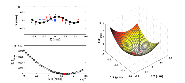
Figure 5: The principal of minimum energy dissipation correctly predicts the displacement and rotation of a self-propelled worm in a 2D anomalous $K$ medium. Simulations confirm that the solution of the equations of motion coincides with the minimum energy dissipation. A. An undulating body with sinusoidal shape moving according to the equations of motion. Red arrows represent the drag force acting on each point. The “CoM” (blue circle) moves with velocity V (blue arrow) such that the net drag force is zero. B, C. The corresponding energy dissipation landscape based on a sweep of displacements (x,y) in a plane (B) and rotation in the plane (C). In both plots the minimum energy dissipation is marked in red on the landscape. The motion obtained from the equations of motion (shown in A) is indicated by a blue line. The results agree to within the step size.

IV.3 Modeling worms

A physics simulator like the one described above is useful in cases where the locomotion waveform can be recorded or pre-determined, but intentionally avoids the question of how an object or organism generates its undulation wave. In general, the shape of the body is determined by a combination of (i) internal (molecular or muscle) actuation forces, (ii) physical properties of the body and (iii) external forces from the environment.

Consider again our friend C. elegans. Conveniently, the worm’s neuro-anatomy essentially limits it to bending in two dimensions White et al. (1986); Chen et al. (2006). Nematodes, like other worms, lack any form of rigid skeleton and instead rely on the antagonistic forces of their elastic outer casing (cuticle) and the hydrostatic pressure within their body cavity to maintain their shape. Thus, at the simplest level, the body can be represented by an elastic rod or cylinder with some internally controlled bending along the rod. Alternatively, more elaborate and detailed models are possible that allow for more accurate biophysical and biological grounding.

In the nematode literature, the canonical example is a model of C. elegans locomotion due to Niebur and Erdös Niebur and Erdös (1991), which is based on exactly these principles. Their 2D model approximates the body as an elongated rectangle represented by two rows of points along its outline. Adjacent points are connected by springs (representing the cuticle) and are pushed apart by pressure forces. This body also behaves effectively as an elastic rod with a characteristic persistence length. Note that until now, we have not evoked any low Re considerations (except that we have not endowed our ‘rod’ with any mass).

The low Re physics does come in when solving for the changes of shape and position of the body. In the above model, points are able to move independently under the action of muscle forces, and modulated by the environment. To solve the model, one can invoke once more the slender body theory and approximations due to Gray et al. Gray and Hancock (1955); Gray and Lissmann (1964), and decompose the forces into tangential and normal components $F_{\parallel}$ and $F_{\perp}$. Much like the physics simulator described above, the zero net force condition can be applied to calculate the velocity of each point along the body. Specifically, we can write write $F_{\rm{drag},i}=-c_{i}v_{i}=-F_{\rm{internal},i}$ along each direction $i$, and since we already have our internal forces, it remains to extract the speeds along each direction $v_{i}=F_{\rm{internal},i}/c_{i}$.

V Sensory integration and closed loop control

To complete the model of an undulating system, one may also include the active elements that induce and control the bending of the body. This may be the molecular biophysics underlying force generation in flagellar motion, or a much higher level model of brain and body control in an undulating animal. Either way, one can think of a motor control system as consisting of a control signal that drives actuators or motor elements to control the shape of the body, subject to environmental forces. In animals, the control signal is generated by the nervous system; the actuators are muscles; and feedback messages are generated either by the body (signals that sense the state of the muscles as well as the orientation and shape of the body) or by other sensory perception (vision, etc.). For example, when we lift a heavy object or push against a wall, the body senses a strong resistance from the environment and can relay this to the nervous system which, in turn, can alter or modulate the neural control. Thus, in this example the neural signal can be thought of essentially as a centrally controlled system with some feedback. It turns out that the vast majority of animal motor control systems contain such neural “control boxes”. Since most muscle behavior consists of rhythmic motion, the underlying neural control generates rhythmic patterns of activity. Neural circuits that generate rhythmic patterns of activity even when completely severed from the rest of the body are dubbed central pattern generating or CPG circuits Marder and Calabrese (1996); Marder (2000); Harris-Warrick (1993).

The fact that a CPG functions in isolation suggests that it can also be modeled in isolation. Indeed, traditionally, most animal motor control models (locomotion included) tended to be limited to a bottom-up model of internal neuronal or neuro-muscular dynamics. These models are then complemented by top-down models of the physical aspects of locomotion (e.g., the aerodynamics of flight, the mechanics of legged locomotion and so on). The underlying assumption here is that, to a first approximation, the neuronal control can be treated as a stand-alone control unit and hence decoupled from the physics of the body and environment.

When then does the physics matter sufficiently to justify an integrated neuro-mechanical model? In what follows, we describe two examples of swimming undulators: the lamprey, and C. elegans. In the lamprey, the vast majority of modeling has focused entirely on the isolated neural control of locomotion. Recent exceptions are beginning to highlight the role that physics plays in the locomotion and are perhaps opening new avenues of investigation of this classic model system. In C. elegans, the low Re physics has long been recognized to play a significant role, but models have still tended to decouple the nervous control from the mechanics. Here too, experiments and models are moving increasingly in a direction of an integrated study of the entire locomotion system, bottom-up and top-down.

V.1 A high Re example: Lamprey swimming

The lamprey is a primitive, eel-like aquatic vertebrate that can reach up to one meter in length. It swims by propagating lateral undulations with increasing amplitude along its body (from head to tail). Lampreys have a brain and spinal cord with a relatively complex nervous system. The spinal cord serves to relay information between the brain and body, but is also capable of complex dynamic behavior. In the 1980s it was shown that the basic neural activity pattern responsible for locomotion could be produced by the isolated spinal cord Cohen and Wallen (1980), without any input from the brain or from sensory pathways. This became the canonical example of a vertebrate CPG circuit Cohen et al. (1982); Cohen (1987a); Kopell and Ermentrout (1988); Ermentrout and Kopell (1994); Grillner et al. (1998).

It was further shown that the lamprey CPG consists of a sequence of semi-independent neural oscillators that are capable of independent pattern generation, but are coupled to each other in such a way that the correct phase lag between adjacent units is preserved Cohen (1987b). Thus, the CPG circuit can generate stable rhythmic activity (at swimming frequencies) that propagates along the spinal cord, and where each ‘segment’ along the body exhibits anti-phase oscillations between the left and right sides of the body (so that when connected to the muscles, one side would contract when the opposite side relaxes). In most CPG circuits, the prevalent model of anti-phase oscillators relies on the half center oscillator Grillner et al. (1998); Churchland and Sejnowski (1992), which consists of two units that are coupled via reciprocal inhibition (as shown schematically in Fig. 6A). These units typically represent separate pools of neurons (as they do in the lamprey). External driving forces and/or internal dynamics modulate the activity to generate rhythmic, out of phase activity.

Figure 6: Schematics of neural oscillators for motor control. A. The half-center oscillator is the simplest central pattern generating circuit (excluding intrinsically oscillating neurons) and consists of two mutually inhibiting neurons. An additional requirement is that the neurons can be released from, or are able to escape from, the inhibition. An example of a release mechanism is synaptic fatigue, where the inhibition wears out over time. B. Simplified nematode oscillator network (adapted from Ref. [Stretton et al., 1985]). (E)xcitatory neurons innervate the (I)nhibitory neurons which in turn relay the inhibition to the opposing excitatory neuron. C. The lamprey segmental oscillator (adapted from Ref. [Ijspeert et al., 1999]) is more complex, but functions along similar principles. It consists of motor neurons (MN) along with three classes of interneuron (IN), with CIN providing the contralateral inhibition.

Early models of the lamprey spinal cord relied on exactly these principles, and have led to important advances, both in the study of the lamprey and other nervous systems Cohen et al. (1982, 1992); Ijspeert et al. (2005), and in our understanding of coupled oscillator systems in nonlinear dynamics Kopell and Ermentrout (1986, 1988); Ermentrout and Kopell (1994). While the lamprey swimming CPG circuit (Fig. 6C) looks rather complicated, the motif of reciprocal inhibition that is required for generating oscillations is not very different from the minimal circuit in Fig. 6A. The circuit includes both excitatory and inhibitory pools of neurons that innervate motor neurons that connect to the muscles. Excitatory interneurons (EIN) provide the excitation to switch the circuit on; contralateral inhibitory interneurons (CIN) provide the cross inhibition, and lateral inhibitory interneurons (LIN) help to terminate contraction of each side Ekeberg (1993). This principle is demonstrated in an elegant robotic instantiation by Auke Ijspeert et al. Crespi et al. (2005), that builds on the integrated neuro-mechanical model of lamprey swimming due to Ekeberg Ekeberg (1993).

Over the years, as models of the lamprey motor control have become more refined and sophisticated, research has increasingly focused on modeling the modulations of the swimming rhythms by input from the brain, from sensory neurons and by the local action of chemicals (so-called neuromodulators) and even modulation by proprioceptive inputs, but of these, the role of sensory effects are least understood Cohen and Boothe (1999). To shed some light on the effects of sensory feedback, Simoni and DeWeerth Simoni and DeWeerth (2007) have recently introduced a neuromechanical lamprey model with sensory feedback to study synchronization effects between the CPG circuit and the mechanical resonance of the body. In principle, this approach, if further complemented by an understanding of the fluid dynamics, should lead to further progress in understanding how the lamprey and other systems exploit the physics of the environment to modulate their internal neural dynamics and motor control.

V.2 A low Re example: C. elegans

Imagine a system in which the neural control is driven directly by sensory signals (such as reflexes). Such a neural system would completely fail in the absence of a body. Surprisingly, such appears to be the minimal model describing C. elegans locomotion Niebur and Erdös (1991); Berri et al. (2009); Boyle et al. (2009). We have already briefly described some of the worm’s means of locomotion and its exploitation of the environment to generate thrust (see Secs. III.2 and IV), but here we focus on the internal (neural) control of the worms’ undulations.

This tiny nematode worm has an invariant anatomy that consists of a mere 959 cells in the adult. Of these, about a third (302 cells) are nerve cells or neurons. These make up a simple nervous system that is distributed throughout the animal. Remarkably, the nervous system appears invariant. In other words, the connectivity diagram or neural circuitry is the same across worms. This connectivity diagram was meticulously mapped out White et al. (1986); Chen et al. (2006) and is the starting point for understanding the worm’s behavior.

Locomotion is the worm’s principal motor activity and mediates everything the worm does, from foraging to mating. Thus, it is not surprising that of its 302 neurons, around 200 are involved in locomotion. Of those, about 50 are directly responsible for the generation of undulations and their backward propagation down the body, i.e., the generation of forward locomotion. (The worm can also move backwards, propagating waves from tail to head, but this behavior relies on a different set of neurons). To put these numbers in perspective, the human brain contains of the order of $10^{11}$ neurons and an insect such as the tiny fruitfly has about $10^{5}$. Thus, while the nervous systems of most animals (including lamprey and even the fruitfly) rely on large populations of neurons to perform processing, in C. elegans single neurons must do the same job.

When nematodes are placed in environments with different viscous, visco-elastic or gel properties, the parameters of their locomotion wave change quite significantly. For instance on agar gels, the worms exhibit slow ($\sim$0.5Hz) short-wavelength undulations (with the body length spanning about 1.5 wavelengths), whereas in watery environments, they appear to thrash, i.e., undulating much more quickly (at $\sim$2Hz) with a wavelength of just under twice the body length. In fact, the entire range of intermediate behaviors can also be obtained in environments with various degrees of visco-elasticity Berri et al. (2009). In principle, the observed change in behavior could be the result of internal changes to the neural circuit (e.g., by neuromodulators, or sensory pathways that activate different sub-circuits). Alternatively, the entire change in behavior may be down to changes in the physical interaction between body and environment.

To shed light on this problem requires a closer look at the locomotion nervous circuit of the worm. Unlike vertebrates, the worm does not have a spinal cord, but it does have an analogous ventral cord which contains the locomotion motor neurons, and so we shall focus on it. First, one may look for evidence of characteristic motifs along the ventral cord that are expected to generate rhythmic activity, such as reciprocal inhibition. This typically requires breaking up the circuit into small units (analogous to segments or vertebrae in the lamprey). Unfortunately, even this first step is not a trivial task, since the nervous circuit of the worm contains very different numbers of neurons on different sides of the body, and so is not naturally divisible into repeating units. Based in part on data from related nematodes, in which direct recording from neurons is possible, a model of the generic nematode segmental oscillator (Fig. 6B) was proposed Stretton et al. (1985). This circuit bears a distinct resemblance to the simple half-center oscillator in Fig. 6A, except that the inhibition is mediated via distinct inhibitory neurons. Nonetheless, for a combination of reasons, questions have been raised about the ability of this circuit to support a CPG network.

One may therefore ask what would be a working model of the locomotion in the possible absence of a CPG mechanism. One interesting conjecture is that the worm may use a sensory feedback mechanism as the primary driver of its neuronal oscillations. Weight is given to this hypothesis by several models of the worm’s locomotion that are grounded in its anatomy and successfully produce oscillations by means of mechanosensory feedback Bryden and Cohen (2008); Karbowski et al. (2008). How would such a mechanism work? We begin by discussing the worm’s so-called crawling behavior (short wavelength undulations observed on agar). This was addressed by the first model of C. elegans locomotion due to Niebur and Erdös Niebur and Erdös (1991). Their model of the worm’s body was introduced in the Sec. IV.3, but they also proposed a simple model nervous system.

This model involved a hypothetical CPG circuit in the worm’s head, allowing it to generate a sinusoidal trajectory that was then preserved by strong lateral resistance, due to a very stiff groove (high $K$). The worm’s shape was therefore determined by the shape of the groove, and the model nervous system was then responsible for generating muscle contraction down the body, pushing the worm forwards. To control the rhythmic muscle activity and rhythmic underlying neuronal activity, the neurons in the model were endowed with so-called stretch receptors, or mechano-sensitive ion channels that activate an ionic current in response to stretch. The current then activates that neuron, and local muscle contraction is induced. If muscles on one side of the body are maximally contracted, the tissue on the other side is maximally stretched. Crucially, the model assumes that the stretch receptor signal is transmitted some distance forward from the site of the stretch: The existence of a set distance between the stretch detection and the ensuing contraction can result in the propagation of the undulation in the desired direction (from head to tail). This integrated neuromechanical model was able to reproduce the crawling behavior on agar if the groove was assumed to be sufficiently stiff (with very high $K$). The main limitation of this model was the fact that it only worked for high $K$, and therefore failed to produce any oscillations in a virtual environment equivalent to water. At the time however, it was believed that the worms swimming in water and crawling on agar were separate locomotory gaits (like a horse’s trot and gallop) White et al. (1986). One might therefore conjecture that the two behaviors would involve separate neural mechanisms.

So how does an organism with such a limited neural circuit adapt its locomotion waveform in environments with drastically different properties? The fact that the worm is capable of a continuous range of behaviors suggests that it relies on a continuous modulation of a single mechanism grounded in a single circuit. The most parsimonious explanation would involve an effectively unchanged neural system, whose activity is modulated solely by the physics of the environment. This is not unlikely in a low Re environment. In fact, passive flagella of bacteria also exhibit shape changes when the viscosity of their environment is increased Schneider and Doetsch (1974), and even more pronounced effects can be observed in the waveform of a sperm’s flagellum (where active bending occurs along the length of the filament) Brokaw (1966). This suggests that a modulation of waveform by physical forces is worth exploring. Within the context of a neural system, one would expect a mechanism driven by sensory-feedback to be more naturally suited to direct modulation by the physics of the environment than a CPG controlled one. Furthermore, one would expect that without the constraints of an internally clocked system, the modulation could take place over a wider dynamic range. Such a mechanism would need to explain changes in frequency, amplitude and wavelength of undulations Berri et al. (2009).

It is not surprising that an increase in mechanical load on the body and muscles (with increased viscosity or visco-elasticity) will result in slower contraction. To explain the corresponding decrease in wavelength and amplitude, it is convenient to imagine the body initiating an undulation from a straight line configuration. The higher the environmental resistance, the harder it is for the body to bend. This change is most pronounced in the middle of the body, as bending here requires significant movement of the head and tail. The head, which is strongly activated and has one free end, will react first. At some point the head will be sufficiently bent that the stretch receptors trigger and the direction of bending is reversed. The mid-body meanwhile is still trying to bend in the first direction and will only reverse after some delay. (This assumes that during locomotion, a straight worm is unstable and will tend to bend.) As the viscosity increases, the phase lag between adjacent parts of the body will increase, leading to a shorter and shorter wavelength.

Consider now the average body curvature which increases with viscosity or visco-elasticity. Assuming that stretch receptor signals are integrated over some length of the body, the average curvature will be related to the wavelength of the undulation . Specifically, the higher the curvature, the shorter the wavelength. When the wavelength is short, the stretch receptor integrates over a significant fraction of the wavelength. Thus while some parts of its receptive field will be highly curved, other parts will be nearly straight, or even curved the other way. Conversely, when the wavelength is long, the curvature will be more homogeneous along the receptive field. Thus, while the level of integrated curvature required to cause a reversal of bending will be the same across the different environments, the peak curvature will be greater when the wavelength is shorter.

The above reasoning was used in an integrated neuro-mechanical model of nematode locomotion that reproduced the swim-crawl transition across different environments Boyle et al. (2009). This model is grounded in the known neural circuitry (a variation on Fig. 6B), and does not contain a CPG either in the head or along the body. The only parameter changes required to modulate the locomotion are to the drag coefficients $c_{\parallel}$ and $c_{\perp}$. The key ingredients of the model are bistability in the motor neurons (leading to instability of straight line configurations) and sensory feedback via distributed stretch receptors.

Having reviewed a system that can rely entirely on sensory (proprioceptive) feedback to drive and modulate undulations, you might ask whether this esoteric example is of any interest to the neuroscience community, since, as mentioned above, such extreme reliance on sensory feedback and absence of CPGs is truly unprecedented in the animal world. However, it is important to remember that most living systems combine central control with sensory modulation Wilson (1961); Pearson (1995); YU et al. (1999) and where advantageous, such systems will exploit the physics of the environment. Indeed, more and more, examples are being studied in which sensory-motor control takes over when the CPG activity is somehow disabled YU et al. (1999).

VI Applications to mobile micro- and nanorobotics

In this paper we have focused on a few examples of low Re undulatory locomotion, but the principles, theories and techniques can all be applied to many other situations. There are countless organisms that use undulatory locomotion similar in form to that presented here, over a range of Reynolds numbers and spanning some 6 orders of magnitude in size. Moving to high Reynolds number, for example, means that certain principles (like the scallop theorem) no longer apply but others (like the requirement of symmetry breaking) still do. Here we will begin by introducing some interesting biological examples (taken from our own bodies) of systems that, while incapable of locomotion per se, bear similarities to what we have covered so far. This will be followed by some examples of biologically inspired robotic applications of undulatory locomotion.

It is perhaps not surprising that biology has applied the principles of undulatory locomotion to the task of moving substances around. One example of this is peristalsis, the mechanism by which food is moved through our digestive tract Huizinga and Lammers (2009). Imagine taking a swimmer and attaching it to a solid object at one end. What we are left with is essentially a pump. Our intestine, while anchored in place, generates waves of muscle contraction which pump semi-digested food through our system. The smooth muscle of our intestine can only contract inwards (reducing the radius), but by propagating coordinated waves of activity the food is propelled in one direction by the leading edge of the wave in much the same way that our hypothetical organism in Sec. II.3.2 generates thrust.

Another type of biological pump can be found, among many places, in our trachea (wind pipe). The inside of our trachea is lined with organelles called cilia, which are genetically very closely related to eukaryotic flagella, and possess the same 9+2 microtubule structure Bray (2001). Compared to flagella, cilia are generally shorter and are found in greater numbers. While a flagellum generally produces thrust in the direction of its long axis (like a propeller), cilia generally produce thrust perpendicular to their long axis (like oars). Their asymmetric beating pattern Marino and Aiello (1982) is such that they minimize drag on the forwards stroke and maximize drag on the backwards stroke, thereby generating thrust along the surface from which they protrude. In so doing, they move mucus and dirt away from our lungs ready for expulsion. In fact, cilia perform other roles as well. In many cases they act as sensory organs Bray (2001) (such as the cilia in our ears), but that is outside the scope of this paper. Motile cilia are also found on some micro-organisms like protozoa (unicellular eukaryotes), where they are responsible for locomotion. Their behavior is similar to those in our lungs, except that the flow of fluid in one direction propels the protozoa in the other.

One of the most exciting applications of the theory of undulatory propulsion in recent years is to the field of bio-inspired robotics. Traditionally robots have used wheels or tracks to get around, but neither of these are a great solution to the problem of locomotion in heterogeneous and difficult terrain. Given the success with which biological organisms move around, it is natural to attempt to emulate these behaviors. In many cases, legged locomotion seems like the ideal solution and recent advances suggest that legged robots may soon be sufficiently advanced to handle real terrain. But there are also many cases where undulatory locomotion would be preferable. A snake-like robot Hopkins et al. (2009) may, for example, be able to inspect the inside of narrow pipes, search for survivors among the rubble of collapsed buildings and traverse even the roughest terrain. A snail-like robot (snail locomotion uses a form of undulation) Chan et al. (2005) could climb vertically or even upside down. But a particularly interesting environment in which small, worm-like robots Menciassi et al. (2006) could potentially operate is the human body Chen et al. (2008). Designers of medical technologies constantly strive to find non-invasive (or less invasive) ways to diagnose and repair problems within our bodies, and micro-robots (or even remotely guided bacteria Martel et al. (2006)) are a promising avenue. Undulatory locomotion Behkam and Sitti (2006) is ideally suited to use within the human body as it is generally robust to heterogeneous environments and is non-destructive. While we are still a long way from this final goal, researchers working on small scale undulatory robots are following a number of interesting directions and making strides both on foundational issues and on the non-trivial engineering challenges of miniaturization.

VII Discussion

In this paper, we have gone from reviewing some fundamental physics applied to low Re swimmers, through different simulation approaches, to biological examples of undulating organisms. The field is too vast to have touched on all the research that is relevant and ongoing, so we have chosen to offer only a cursory view of better known systems and results (such as bacterial swimming and lamprey CPGs), and to spend more time on less familiar examples, such as Helmholtz’s minimum energy dissipation theorem, generalizations of the scallop theorem and nematode locomotion.

To the physicist uninitiated in biological parlance, the level of biological detail in some of the examples may appear daunting, or perhaps superfluous. However, one of the key roles of the biological physicist is to tease out the essential features of what can seem an almost arbitrarily complicated system. Therefore, we have not shied away from leaving the physics grounded in at least some of the biological systems in this review. We hope that this approach serves less as a hindrance and more as an invitation to the readers to engage in the larger endeavor that is the interface between physics and biology.