Quasi-periodic oscillations under wavelet microscope: the application of Matching Pursuit algorithm

We zoom in on the internal structure of the low-frequency quasi-periodic oscillation (LF QPO) often observed in black hole binary systems to investigate the physical nature of the lack of coherence in this feature. We show the limitations of standard Fourier power spectral analysis for following the evolution of the QPO with time and instead use wavelet analysis and a new time-frequency technique – Matching Pursuit algorithm – to maximise the resolution with which we can follow the QPO behaviour. We use the LF QPO seen in a very high state of XTE J1550$-$564 to illustrate these techniques and show that the best description of the QPO is that it is composed of multiple independent oscillations with a distribution of lifetimes but with constant frequency over this duration. This rules out models where there is continual frequency modulation, such as multiple blobs spiralling inwards. Instead it favours models where the QPO is excited by random turbulence in the flow.

1 Introduction

One of the most outstanding features of the stellar mass black-hole binaries (BHB) is their rapid X-ray time variability (e.g. van der Klis 1989). This variability consists of aperiodic continuum noise spanning a broad range in frequencies, with quasi-periodic oscillations (QPOs) superimposed. The ‘low frequency QPO’ (hereafter LFQPO) is the one most often seen, and this is at a characteristic frequency which moves from 0.1–10 Hz in a way which is correlated with the energy spectrum of the BHB (see e.g. the reviews by van der Klis 2006; McClintock & Remillard 2006; Done et al. 2007).

The true nature of this LFQPO (or any of the other QPO’s) is still not well understood, and there are multiple suggestions in the literature. The most fundamental frequency is Keplarian, but this is very high, at $\sim 200$ Hz at the last stable orbit for a $10M_{\odot}$ Schwarzchild black hole (Sunayev 1973). Instead, the QPO could be linked to the buildup and decay of ‘shots’ on the longer timescales for magnetic reconnection events (Miyamoto & Kitamoto 1989; Negoro et al. 1994), though to form a QPO probably requires correlation between the shots via an energy reservoir (Vikhlinin et al. 1994). Alternatively, the frequency could be set by modes excited in the accretion disc (Nowak & Wagoner 1995; Nowak et al. 1997), or by one-armed spiral waves in the disc (Kato 1989) or Lense-Thirring precession (Ipser 1996; Stella & Viertri 1998: Psaltis & Norman 2000; Ingram et al. 2009).

Clearly, observational constraints are required in order to distinguish between some of these very different physical models. Firstly, the energy dependence of the QPO clearly shows that the oscillation does not involve the optically thick accretion disc emission but is instead a feature of the higher energy Comptonised tail (e.g. Życki et al. 2007). Therefore all models using a modulation of the thin disc are ruled out. Instead, the QPO must be connected to the hard X-ray emitting coronal material, though the ‘shot noise’ models are ruled out by the observed r.m.s.–flux correlation as this cannot be formed by independent events (Uttley et al. 2005).

More constraints come from the detailed shape of the QPO signal. The most popular method for studying X-ray variability is the Fourier power spectrum density (PSD; see Vaughan et al. 2003 and references therein). This is the square of the amplitude of variability at a given frequency, as a function of frequency, namely $P(f)$. Power spectra from BHB can be very roughly described as band limited noise, with a ‘flat top’ in $\nu P(\nu)$ (equal variability power per decade in frequency) i.e. $P(\nu)\propto\nu^{-1}$. This extends between a low and high frequency break, $\nu_{b}$, below which the PDS is $P(\nu)\propto\nu^{0}$, and $\nu_{h}$, above which the spectrum steepens to $P(\nu)\propto\nu^{-2}$. However, this broadband noise is better described by a sum of 4–5 Lorentzian components (Belloni & Hasinger 1990; Psaltis et al. 1999; Nowak 2000; Belloni, Psaltis & van der Klis 2002). This has the advantage that LF QPO is also well modelled by a Lorentzian, so both QPO and underlying noise can be fitted with the same functions. More importantly, Lorentzians also suggest a physical interpretation of the power spectral components as these are the natural outcome of a damped, driven harmonic oscillator. Each Lorentzian-like structure in a PSD may then be related to a process in the accretion flow, hence X-ray emission $x(t)\propto\sin(2\pi f_{0}t)\exp(-t/\tau)$ where $\tau$ denotes a damping time-scale (Misra & Zdziarski 2008; Ingram et al. 2009).

A Lorentzian has $P(f)=A\Delta f/[(f-f_{0})^{2}+(\Delta f/2)^{2}]$, defined by a centroid frequency, $f_{0}$, a full width at half maximum (FWHM) of $\Delta f$ and amplitude. A ratio of the QPO frequency to Lorentzian FWHM is known as a quality factor, $Q=f_{0}/\Delta f$. The distinguishing feature of the QPO as opposed to the noise components is that its quality factor can be large. All these paramters are correlated in the LF QPO, with the amplitude and quality factor increasing along with the increase in centroid frequency (e.g. Nowak et al. 1999; Nowak 2000; Pottschmidt et al. 2003).

It is obviously important to know what sets the (lack of) coherence of the QPO. Are QPOs composed of a set of longer-lasting continuous modulations or are they rather fragmented in time with frequencies concentrated around the peak QPO frequency? Is there any correlation between observed oscillations or they are preferably excited in a random manner? To answer these questions we need to resolve and understand the internal structure of detected QPOs i.e. to study the behaviour of the QPO on timescales which are short compared to its observed broadening. A continuous modulation would then show up as a continuous drift in QPO frequency with time, while a series of short timescale oscillations will show up as disjoint sections where the QPO is on and off.

One way to do this is using dynamical power spectra (spectrograms; hereafter also referred to as STFT for simplicity). While the actual techniques for this can be quite sophisticated, (e.g. Cohen 1995; Flandrin 1999), in essence, an observation of length $T$ sampled every $\Delta t$ (giving a single power spectrum spanning frequencies $1/T$ to $1/(2\Delta t)$ in steps of $1/T$) is spilt into $N$ segments of length $T/N$. This gives $N$ independent power spectra spanning frequencies $N/T$ to $1/(2\Delta t)$ but crucially, the resolution is now lower, at $N/T$. While this is useful in tracing the evolution of the QPO (e.g. Wilms et al. 2001; Barret et al. 2005), it introduces ‘instrumental’ frequency broadening from the windowing of the data which prevents us following the detailed behaviour of the QPO on the required timescales.

The real problem with such Fourier analysis techniques is that they decompose the lightcurve onto a basis set of sinusoid functions. These have frequency $f$, with resolution $\Delta f=N/T$, but exist everywhere in time across the duration of the observation $t_{dur}=T/N$. In the same way that the Heisenburg uncertainty principle sets a limit to the measurement of momentum and location of a particle, namely $\Delta p_{x}\Delta x\geq h/2\pi$ where $h$ is a Planck constant, there is a Heisenberg-Gabor uncertainty principle setting the limiting frequency resolution for time-series analysis. This states that we cannot determine both the frequency and time location of a power spectral feature with infinite accuracy (e.g. Flandrin 1999).

Instead, if the QPO is really a short-lived signal, we will gain in resolution and get closer to the theoretical limit by using a set of basis functions which match the underlying physical shape of the QPO. This is the idea behind wavelet analysis. For example, one particular basis function shape is the Morlet wavelet, which is a sinusoid of frequency $f$, modulated in amplitude by a gaussian envelope such that it lasts only for a duration $t_{dur}$. The product $f\times t_{dur}$ is set at a constant, fixing the number of cycles seen in the basis function. The lightcurve is then decomposed on these basis functions, calculated over a set of frequencies so that the basis function shape is maintained (i.e. that the oscillation consists of 4 cycles, so low frequencies have longer $t_{dur}$ than high frequencies). The resolution adjusts with the frequency, making this a more sensitive technique to follow short duration signals (e.g. Farge 1992; Addison 2005).

Quite quickly, wavelet transforms gained huge popularity within the astronomical community (e.g. Szatmary, Vinko & Gal 1994; Frick et al. 1997; Aschwanden et al. 1998; Barreiro & Hobson 2001; Freeman et al. 2002; Irastorza et al. 2003) whereas its application in X-ray astronomy was not so rapid. Scargle et al. (1993) used wavelets to examine QPO and very low-frequency noise in Sco X-1. Steiman-Cameron et al. (1997) supplemented Fourier detection of quasi-periodic oscillations in optical light curves of GX 339–4 by wavelets while Liszka et al. (2000) analysed the ROSAT light curve of NGC 5548 in short time-scales. Recent studies of QPOs in X-ray black-holes systems can be found e.g. in Lachowicz & Czerny (2005), Espaillat et al. (2008) and Gupta et al. (2009).

However, the problem is that the basis functions chosen in wavelet analysis may not be appropriate. For example, we assumed above that these functions have a fixed shape, lasting for a fixed number of oscillations at all frequencies. In practice, this may not be the best description of the QPO. Perhaps the QPO is made from a set of signals which have a distribution of durations, where $f\times t_{dur}$ is not constant. We will maximise the resolution with which we can look at the QPO if and only if we use basis functions which best match its shape.

To do this we propose the application of the Matching Pursuit algorithm (MP). This is an iterative method for signal decomposition which aims at retrieving the maximum possible theoretical resolution by deriving the basis functions from the signal itself. We specifically use this as an extension of the wavelet technique by setting the MP basis functions as Gaussian amplitude modulated sinusoids as before, but allowing the product $f\times t_{dur}$ to be a free parameter (Gabor atoms).

We apply both wavelet and Matching Pursuit analysis to zoom in on the detailed structure of the LF QPO. A technical description of these time-frequency techniques we provide in the Appendix. We describe the data used in Section 2. This is a RXTE/PCA observation of the BHB XTE J1550–564 which which displays a strong and narrow QPO at $\sim$4 Hz. Section 3 shows how wavelets and MP give more information than the standard dynamical power spectra. We study wavelet and Matching Pursuit feedback to different QPO models in Section 4 whereas in Section 5 we discuss the new physical insights this gives about the QPO mechanism.

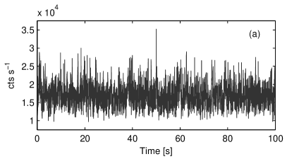
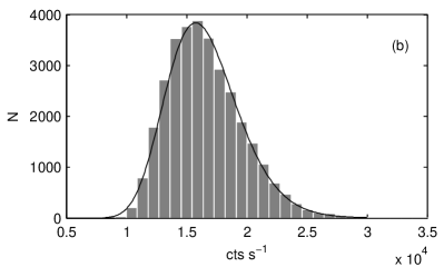
Figure 1: (a) An exemplary 100 s data segment extracted from the light curve of XTE J1550–564 as observed by RXTE/PCA on September 29th 1998. (b) The histogram of data in our sample (1000 s) fitted with a lognormal distribution.

2 Source selection and data reduction

XTE J1550–564 is X-ray nova and black-hole binary discovered on September 6, 1998 (Smith et al. 1998) by All Sky Monitor on-board the Rossi X-ray Timing Explorer facility. A possible optical counterpart was identified to be a low-mass star (Orosz et al. 1998) and the distance to the source was estimated to be about 5.3 kpc (Orosz et al. 2002). A variable radio source was subsequently found at the optical position (Campbell-Wilson et al. 1998) and confirmed by Marshall et al. (1998) based on ASCA observations. Radio jets with apparent superluminal velocities were observed after the strong X-ray flare in September 1998 (Hannikainen et al. 2001), placing XTE J1550–564 among already known microquasars.

The source 2.5–20 keV spectrum was similar to the spectra of sources that are dynamically established to be black-holes. XTE J1550–564 has been observed in the very high, high/soft and intermediate canonical outburst states of black-hole X-ray novae (Sobczak et al. 1999a, 1999b; Cui et al. 1999). The source gained additional support for its black-hole nature due to the detection of a variety of low-$f$ QPOs (0.08–18 Hz) as well as high-$f$ QPOs (100–285 Hz) during some of the PCA/RXTE pointings (Bradt et al. 1993; Cui et al. 1999; Remillard et al. 1999; Wijnands et al. 1999; Homan et al. 2001).

To probe the object quasi-periodic variability in time-scales of seconds we use a pointed observation of the Proportional Counter Array detector of RXTE taken from the public archive of HEASARC (http://heasarc.gsfc.nasa.gov). After Zdziarski & Gierlinski (2004), we selected the PCA data set of ObsID of 30191-01-15-00 containing source observation on 29.09.1998 (MJD 51085) when the binary system was in its very high state (Gierlinski & Done 2003) and displayed narrow QPO feature of quality factor $Q\simeq 11$ (Sobczak et al. 2000).

We reduced the data with the LHEASOFT package ver. 6.6.1 applying the standard data selection: the Earth elevation angle $>10^{\circ}$, pointing offset $<0^{\circ}.01$, the time since the peak of the last South Atlantic Anomaly SAA $>30$ min and the electron contamination $<0.1$. The number of Proportional Counting Units (PCUs) opened during the observation was equal five.

We extracted a light curve in 2.03–13.06 keV energy band (channels 0–30) with a bin size of $\Delta t\!=\!2^{-5}$ s for the first part of PCA observation (2502 s). For the purposes of this paper, we limited our data sample only to the first 1000 s dividing it into ten 100 s ($N=3200$ points) segments for which the wavelet and Matching Pursuit analysis was conducted in detail. An exemplary data segment is presented in Fig. 1a. Our sample returned the mean countrate and r.m.s. variability equal $1.65\times 10^{4}$ cts s^-1 and 18.9%, respectively. The data histogram (Fig. 1b) can be fitted with a lognormal distribution,

$$f(x;\mu,\sigma)=\frac{1}{x\sigma\sqrt{2\pi}}\exp\left[\frac{(-\ln x-\mu)^{2}}{2\sigma^{2}}\right],$$ (1)

and the best fit returns the distribution’s parameters, the mean and standard deviation, equal $\mu=9.698\pm 0.003$ and $\sigma=0.184\pm 0.002$, respectively, where the errors are given at 99% confidence level (see also Uttley et al. 2005 for a detailed discussion on X-ray light curve distribution).

We computed Fourier power spectra using the powspec subroutine in HEASoft package with Poisson noise level subtraction applied. STFT spectrogram plots are derived based on the Matlab${}^{\mbox{\small\textregistered}}$ Signal Processing Toolbox ver. 6.9. For the wavelet analysis the Time-Frequency Toolbox (http://tftb.nongnu.org) was used whereas all results corresponding to the Matching Pursuit signal decomposition were computed using MP ver. 4 code provided by Piotr Durka of the Department of Biomedical Physics at Warsaw University, Poland (http://www.eeg.pl/software).

3 Time-frequency analysis of 4 Hz QPO structure

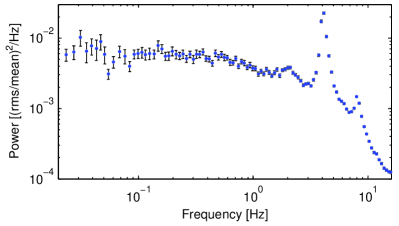
Figure 2: Power spectral density plot calculated based on the entire light curve. Main QPO feature is well detected at the frequency of 4 Hz.

Fig. 2 displays the Fourier power spectral density (PSD) calculated from 78 averaged spectra based on 1024 point data segments. A QPO peaking at a frequency of 4 Hz is clearly evident together with its harmonic structure, and r.m.s. variability calculated in a 3.5$-$5 Hz frequency band equals 12.1%.

We use the first 100 s of data (Fig. 1a) to compare the three different time-frequency techniques. The upper plot in Fig. 3 shows a standard STFT spectrogram, computed on a 1.44 s long rectangular (sliding) window. Thus all oscillations of lifetime shorter than $\sim\!1.44$ s are smeared, and the frequency resolution is 0.7 Hz, comparable to the FWHM of the QPO. The QPO appears to be fairly continuous thoughout the dataset, with small excursions around 4 Hz.

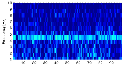
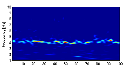
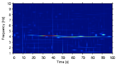
Figure 3: Time-frequency analysis performed for the XTE J1550–564 light curve presented in Fig. 2a: (upper, a) Spectrogram calculated for the first 100 s long data segment revealing QPO activity around a central frequency of 4 Hz (46 point sliding window); (middle, b) the corresponding wavelet power spectrum derived with a Morlet analysing function; (bottom, c) Matching Pursuit decomposition (based on $3\times 10^{6}$ atom dictionary) displayed as energy density $(Ex)(t,f)$ (Eq. 14) uncovering the main quasi-periodic components located mainly between 3.7–4.7 Hz. For all figures colour coding is assumed as follows: increasing values of the STFT/wavelet/MP power (energy density) are denoted by a gradual brightening of the colour, i.e. from dark blue, yellow to red (colour values not in scale).

By comparison, the middle panel of Fig. 3 shows the wavelet power spectrum using the Morlet wavelet basis functions, i.e. modulated sinusoid confined by a Gaussian envelope, $\psi(t)=\pi^{-1/4}e^{i(2\pi f_{0}t)}e^{-t^{2}/2}$, with $2\pi f_{0}=6$ to make each wavelet last for about 4 cycles irrespective of the timescale $t$ for the oscillation. At the QPO frequency of 4 Hz (wavelet scale $a\!=\!0.2427$) the wavelets can resolve signals which last for 1.44 s. Across the QPO width, the wavelet window changes its duration from 1.63 s at 3.5 Hz to 1.14 s at 5 Hz causing a continuous change of frequency resolution from 0.61 Hz to 0.88 Hz, respectively. This gives a better view of the detailed structure of the QPO than the STFT spectrogram, but still limits our view of the detailed composition of the QPO signal to half that of the QPO’s FWHM. Nontheless, this is already able to show that the apparently continuous QPO in the STFT result is actually composed of distinct events.

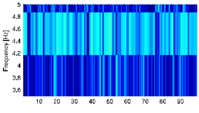
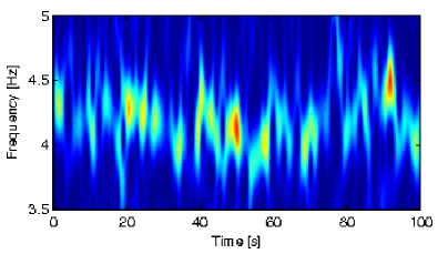
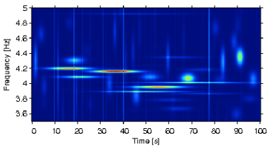
Figure 4: As in Fig 2, but zooming in on the 3.5–5 Hz frequency band dominated by the QPO.

Results from the MP algorithm (Section A.2) are shown in the bottom panel of Fig. 3. This is deconvolved using 500 iterations and displayed as energy density (Eq. 14). This is equivalent to saying that the signal is approximated by 500 separate Gabor atoms (hereafter the term atom will be used interchangeably). Together these account for over 95% of total signal power, or speaking conversely, we can reproduce the entire light curve in 95% based on 500 fitted Gabor atoms (figure not shown). The energy density has been displayed with a linear scale in order to show the time-frequency distribution of the strongest events.

Fig. 4 shows the detailed structure of the QPO (the 3.5–5 Hz band) derived from each of these techniques. This immediately shows the progressive increase in time–frequency resolution from STFT to wavelet to MP analysis. Since MP algorithm scans the whole stochastic dictionary for the best matching Gabor functions to the signal, we gain a new opportunity to represent the QPO structure by a number of localised periodic functions as defined by Eq. (7). The MP map shows that much of the power of the QPO signal in these data is made from 6 to 10 periodic oscillations around 4 Hz, with life-times between 20–60 s. We will return to this result later.

The underlying broadband continuum noise (dominated by the intrinsic variability rather than purely Poisson statistics, see Fig. 1) is also present in all these plots. This appears in the STFT as the gradation of background colour from pale to dark from the bottom (1 Hz) to the top (10 Hz) of Fig. 3a. In the wavelets, this is seen as pale, random smudges around 1$-$3 Hz (Fig. 3b), whereas in MP they are very short-lived signals (less than 0.5 s) forming vertical features across the plot.

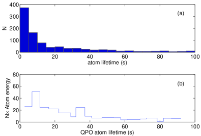
Figure 5: The upper panel shows the histogram of atom life-times as calculated by the MP decomposition within the 3.5$-$5 Hz band. This clearly peaks at short timescales, but extends continuously up to the longest timescales sampled by the data. The lower panel shows the power carried by QPO atoms of each timescale (see text on atom selection). Unlike the atom lifetimes, this does not peak at zero, but instead shows that most of the QPO power is carried by oscillations lasting $\sim$5$-$10 s.

4 Detailed QPO structure from Matching Pursuit

We can quantify the composition of the QPO by showing the distribution of the life-times of 500 Gabor atoms found in the MP decomposition accumulated for ten segments of XTE J1550–564 data in 3.5$-$5 Hz band (Fig. 5a). These show a continuous distribution of lifetimes, peaked at zero but extending out to the longest timescales sampled by the data. Fig. 5b shows the distribution of power carried by QPO atoms of each lifetime (sum of atom energy times number of atoms over all the events in the time bin of that duration). By QPO atoms we define these events distributed between 3.7$-$4.7 Hz and exclude these with a duration below 0.5 s, or with energy which is less than the events in the 2.5$-$3 Hz bandpass (reference red-noise level; see Fig. 2) as both of these will predominantly trace the broadband noise.

We found that the largest number of atoms (more than half of the total 500 per data segment) are characterised by a time duration of 0.5$-$3.5 s, but that these together carry only half the energy of the strongest 10 atoms, which have lifetimes of 20$-$60 s (see Fig. 4c). On the other hand, Fig. 5b reveals that the majority of QPO power is carried by QPO events with a duration of between 5–10 s.

We now explore to what level the results can distinguish between different models for the broadening of the QPO signal.

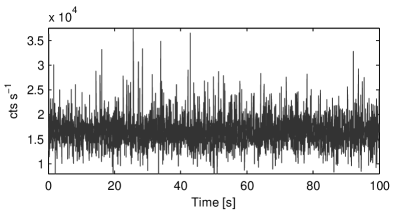
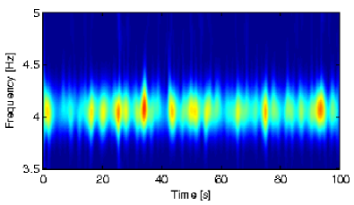
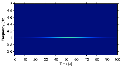
Figure 6: Simulated QPO signal (a; upper panel) which is fully coherent and single frequency but with random amplitude modulation. The middle panel (b) shows the wavelet decomposition. This is not dissimilar to that from the real data in Fig. 4b, though there are fewer large gaps and the derived frequency is more stable. The bottom panel (c) shows the MP decomposition of the same signal. This is clearly different to that of the real data in Fig. 4c, ruling out this QPO shape. Colour coding of a wavelet and MP map assumed the same as described in a caption of Fig. 3.

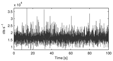
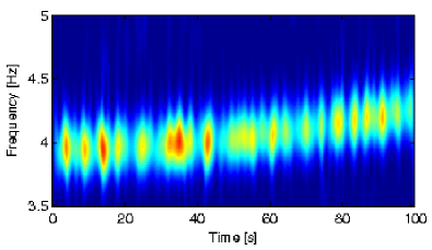
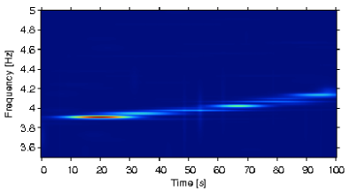
Figure 7: As in Fig. 6, but for a simulated QPO signal which is a fully coherent chirp signal, with frequency increasing with time from 3.9 to 4.2 Hz. A smooth frequency drift is readily apparent in both wavelet and MP maps, unlike the data shown in Fig. 4b and 4c. Colour coding of a wavelet and MP map assumed the same as described in a caption of Fig. 3

4.1 Coherent, single frequency signal with amplitude modulation

Continuous amplitude modulation of a single frequency sinusoid will result in a broad peak in a power spectrum. We simulate this by generating a single sinusoid modulation $y(t)=A\sin(2\pi f_{0}t)+C$ over 100 s with sampling time of $\Delta t=2^{-5}$ s, $f_{0}=4$ Hz, and a constant value of $C=1.65\times 10^{4}$ cts s^-1. The amplitude $A$ is taken as a random variable from the lognormal distribution as fitted to the XTE J1550$-$564’s histogram (see Fig. 1b and Sect. 2 for details). For $y(t)$ we perform its exponential transformation, namely $\exp[y(t)]$, which accounts for a non-linear type of variability present in X-ray light curves of accreting black-hole systems (Uttley & McHardy 2001; Uttley, McHardy & Vaughan 2005). In this point we ensured the signal would have a zero mean and its variance to be such to obtain (after the above transformation and Poisson noise inclusion) a similar degree of r.m.s. as observed for the entire XTE J1550–564 data sample as well as to match r.m.s. variability in the QPO band (3.5$-$5 Hz).

Fig. 6a displays a simulated signal, whereas Fig. 6b reveals the wavelet power spectrum. The spectrum is similar to the XTE J1550–564 wavelet map, but the MP decomposition is clearly different to that in Fig. 4c. The first iteration returned a $\sim$85 s long Gabor atom exactly at a frequency equal to the assumed $f_{0}$, carrying about 85% of the signal energy and dominating over the rest of the fitted atoms.

Therefore the MP decomposition clearly rules out a QPO signal formed solely from amplitude modulation as the real data cleanly show multiple strong Gabor atoms with frequencies between 3.7–4.7 Hz.

4.2 Coherent chirp signal with amplitude modulation

Physical models for the QPO involving blobs spiralling inwards should produce a monotonically increasing frequency signal, otherwise known as a chirp (e.g. Turner et al. 2006; Mhlahlo et al. 2007).

We repeate the experiment above, but with a chirp signal where $y(t)=A\sin[2\pi f(t)t]+C$ and $f$ changes continuously between 3.9 and 4.2 Hz. Fig. 7 shows that again the amplitude modulation can be easily captured in the wavelet map, but it leaves no impact on frequency. In MP map, the continuously changing frequency is fitted with separate atoms (see Sect. A.2.4 for more details on Fig. 7c construction) which trace the drift. The lifetimes of the individual atoms are around 10–20 s and show that the data can distinguish between frequencies separated by $\sim 0.03-0.06$ Hz, i.e. approximately an order of magnitude better than the wavelet technique at these frequencies.

Again, this MP map is quite unlike that of the real data shown in Fig. 4c.

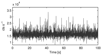
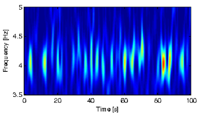
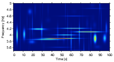
Figure 8: As in Fig. 6, but for a simulated QPO signal which is composed of separate oscillations which last for a timescale randomly distributed between 0-3 s followed by a wait time which is randomly distributed between 0-2 s. Each oscillation has random phase and amplitude but is at a fixed frequency of 4 Hz. The upper panel (a) shows an exemplary light curve. The middle section (b) displays a corresponding wavelet map, while the lowest panel (c) shows MP decomposition. Both these are rather similar to those from the real data in Fig. 4b and 4c. Colour coding of a wavelet and MP map assumed the same as described in a caption of Fig. 3

4.3 Short lifetime, random amplitude signals

The tests described above clearly show that the QPO signal in the data is not given by a single frequency. There are multiple frequencies present in the dataset, but these frequencies do not show any systematic, long timescale trend such as a chirp.

This seems to fit most easily into a picture where the QPO is composed of separate events with shape rather similar to that of the Gabor atom i.e. a single frequency lasting for some timescale $t_{\rm qpo}$ which varies. This would fit quite well into models where the QPO can be randomly excited by turbulence, and last for some timescale before getting damped out. The specific LF QPO model of Ingram et al. (2009) has a vertical, Lense-Thirring precession of the hot inner flow. This will be damped on a viscous timescale, which is of an order $\sim 3$ s for typical parameters.

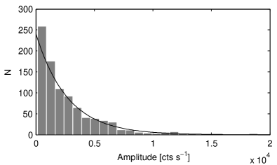
Figure 9: The distribution of amplitudes for QPO Gabor atoms extracted from Matching Pursuit analysis of XTE J1550$-$564 light curve in 3.7$-$4.7 Hz frequency band. The solid line denotes the exponential distribution fitted to the data.

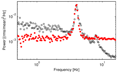
Figure 10: The comparison between power spectral density caclulated for XTE J1550$-$564 (open black circles) and simulated signal as described in Sect. 4.3 (filled red circles).

Here, we approximate this physical picture by assuming that $t_{\rm qpo}$ varies uniformly between $(0,3]$ s and that after each QPO event there is a waiting time of $t_{\rm break}$ randomly distributed in the $(0,2]$ s interval. Therefore the QPO is $\mbox{qpo}(t)=A\sin(2\pi f_{0}t+\phi)+C$ where $f_{0}=4$ Hz and a phase is randomised for every new QPO. As previously, we assume the amplitude to be a random variable, however this time drawn from the exponential distribution,

$$f(x;\mu)=\frac{1}{\mu}\exp\left(-\frac{x}{\mu}\right),$$ (2)

fitted to the histogram of amplitudes derived for QPO atoms (3.7$-$4.7 Hz) from the XTE J1550$-$564 data, where we obtain $\mu=2692^{+245}_{-217}$ at the 99% confidence level (Fig. 9). During the breaks we approximate signal value by a random variable drawn from lognormal distribution and we follow the signal transformation as described in Sect. 4.1.

The above construction of simulated signal allows us to account for a general countrate distribution to resemble that in XTE 1550$-$564 light curve as well as to approximate more adequately the amplitudes of simulated quasi-periodic events. Fig. 8a displays an examplary 100 s signal obtained in the above manner. During the simulation we assumed the r.m.s. variability in 3.5$-$5 Hz band to match closely 12% as derived from the XTE J1550$-$564 data. In Fig. 10 we compare both Fourier power spectra, i.e. for the X-ray source and simulated signal (here taken to be 1000 s long). The plots indicate on very good qualitative agreement between the original and simulated QPO feature in the frequency domain, though it is straighforward to note that our simulation does not correctly reproduce broad-band red-noise variability as observed in XTE J1550$-$564.

Encouraged by the above agreement, we zoom in on the internal structure of our simulation by performing wavelet and Matching Pursuit analysis as previously (Fig. 8), and we find that both maps provide the results which look very similar to that from the real data (cf. Fig. 4b and c).

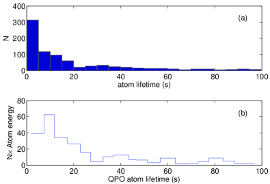
Figure 11: As in Fig. 5, histograms of atom lifetimes and energies for the simulated signal as described in Sect. 4.3. Bottom panel refers to QPO atoms defined in 3.7$-$4.7 Hz band, excluding these events of duration less than 0.5 s and of atom energy lower than in 2$-$3.7 Hz and 4.7$-$5 Hz bands.

More quantitatively, Fig. 11 shows that the distributions of atom lifetimes and energies are also remarkably well matched by the simulation. Even though the signal is made from separate oscillations with life-time of less than 3 s, an MP decomposition displays a number of longer lasting atoms, e.g. of lifetimes between 40$-$80 s. Since this issue requires a better understanding, we examined the MP response to the set of various test signals containing different noise levels, amplitude distribution, variable frequency and/or constant phase for separate qpo$(t)$ events. In conclusion, we have noticed that the longer lasting atoms can be fitted to the data by an MP algorithm making use of an atom concatenation process. In this case, a number of shorter lasting oscillations characterized by very similar phase and frequency (not amplitude!) can be linked together into one longer atom. Therefore, e.g. a 60 s long atom can describe, say, three to five $\sim$3 s oscillations, and our inability to distinguish among them refers to the limited time-frequency resolution of the Matching Pursuit algorithm.

Similarly, while the simulation has only one constant frequency signal, there is a spread in frequency in the MP decomposition which matches that seen in the data.

The low-frequency QPO seen in the real data can be well described by a signal which consists of random, discrete events at a single frequency, with a spread in lifetime and amplitude.

5 Discussion and Conclusion

Quasi-periodic oscillations observed in the power spectra of many accreting compact objects still remain the most intriguing puzzle. Since high-frequency QPOs are generally thought as the most attractive landmark feature used in testing the behaviour of matter in the very strong gravitational field (e.g. Kluzniak & Abramowicz 2001; Rebusco & Abramowicz 2006), on the contrary, the low-frequency QPOs have been found to be more enigmatic in their nature (Casella et al. 2006). For the latter, a quantitative analysis has been a dominant tool towards our comprehension of the global QPO properties (e.g. Cui et al. 1999; Sobczak et al. 2000).

The presence of broad peaks in the Fourier power spectra fitted with Lorentzian profiles suggests a possible mechanism of X-ray engine at work: damping of locally emitted radiation at the very short time-scales (e.g. Misra & Zdziarski 2008). The position of QPO peak frequency varies in time, generally being drifting between 0.1$-$10 Hz (van der Klis 2005, 2006). It has been suggested it may be correlated with both underlying geometry of the inner flow, and accretion rate, thus with the spectral state of the source (e.g. Di Matteo & Psaltis 1999; Dutta et al. 2008; Qu et al. 2010). The r.m.s. variability of LF QPOs is also significant and in some cases exceeds 10%.

The successful modelling of this QPO phenomena requires a sophisticated approach which would include acceptable model’s results not only in the reproductions of the light curve and Fourier PSD, but also in providing an agreement in a function of energy (e.g. Sobolewska Życki 2006). Such attempts have been so far conducted on many occassions (e.g. Giannios & Spruit 2004; Machida et al. 2006; Machida & Matsumoto 2008). Fundamental and dynamical Fourier analysis of X-ray light curves gained a leading position in spoting the existence and evolution of QPOs (e.g. Galleani et al. 2001; Pottschmidt et al. 2003; Barret et al. 2005) but failed in delivering the satisfactory answer on the physical structure due to insufficient resolution. On the hand, the application of new time-frequency methods for X-ray time-series analysis (e.g. by wavelet approach) initiates a novel look at the data and brings an opportunity for testing QPO models in a new space of parameters (e.g. Steiman-Cameron et al. 1997; Parker 1998; Lachowicz & Czerny 2005).

In this paper we have applied the Matching Pursuit method for signal decomposition and shown how MP technique can give much better resolution in the time-frequency plane to study the evolution of the low-frequency QPO seen from black hole binary systems. We have used data from the bright transient systems XTE J1550$-$564 to illustrate this with an observation taken in the very high state (aka the steep power law state) where the QPO is strong and relatively coherent.

The Mathching Pursuit decomposition clearly rules out several potential origins for the broadening of the QPO signal. The ‘quasi’ nature cannot be due to a single frequency, coherent oscillation with amplitude modulation, nor can it be a long timescale ($\sim$100 s) systematic change in frequency (chirp signal). Instead, it is well matched by a series of discrete oscillations, with life-times between 0–3 s, each with random phase and amplitude but fixed frequency.

Physically, this is consistent with models of the QPO where it is excited by random turbulence. In particular, the Lense-Thirring precession model of Ingram et al. (2009) can fit nicely into this picture, where the vertical precession is excited by the large scale stochastic turbulence generated in the accretion flow. The timescale for decay of the vertical precession should be related to the viscous timescale of the flow. In the Ingram et al. (2009) model, a 4 Hz QPO would be associated with an outer radius of the hot flow of $\sim 10R_{g}$, so should have a viscous timescale of $\sim 2-3$ s for the typical parameters used by Ingram et al. (2009).

The application of Matching Pursuit opens a brand new opportunity for studies of LF QPOs in the time-frequency domain. It encourages for revision of archival data of other BHB which display narrow QPOs in their Fourier power spectra. By increased time-frequency resolution provided by MP it is possible to diferentiate amongst various QPO models, as demonstrated in this paper. Therefore, the Matching Pursuit analysis may bring us much closer towards understanding of the underlying physical properties of the QPO phenomenon.

Appendix A Time-Frequency Analysis

A.1 Spectrogram and wavelet analysis

In X-ray time analysis the wavelet transformation constitutes an alternative tool for signal decomposition when confronted with the classical approach based on the Fourier transform (PSD). In the latter, a signal is analysed with the basis functions $\psi\propto e^{{\rm i}ft}$. It detects strictly periodic modulations (with period of $1/f$) buried in the signal. Therefore, no information about time-frequency properties is available.

A simple solution to this problem has been found via the application of Short-Term Fourier Transform (STFT). Basic concept standing for this method is to divide signal into small segments and calculate for each of them Fourier transform. The signal analysis performed using spectrogram, i.e. $|$STFT$|^{2}$ often blurs all signal oscillations of life-times less than the duration of a segment causing a loss of significant information.

The wavelet analysis treats this problem more accurately as a basic concept standing for its usefulness relay on probing time-frequency plane at different frequencies with different resolutions. The wavelet power spectrum for a discrete signal can be defined as the normalised square of the modulus of the wavelet transform $\xi|w_{n}(a_{m})|^{2}$ where $\xi$ stands for normalisation factor and $w_{n}(a_{m})$ a discrete form of the continuous wavelet transform (Farge 1992; Torrence & Compo 1998; Lachowicz & Czerny 2005). It is attractive to adopt a Morlet wavelet to probe quasi-periodic modulations. Since Morlet wavelet oscillates due to a term $\propto e^{{\rm i}t}$, it is perfectly suited for this task.

A.2 Matching Pursuit algorithm

A.2.1 Parlez-vous français?

Signal time-frequency analysis can be compared to speaking in a foreign language. In each language we use words. Words are needed to express our thoughts, problems, ideas, etc. By a smart selection of proper words we can say and explain whatever we wish. A whole collection of words can be gathered in the form of a dictionary. One can express simple thoughts using a very limited set of words from a huge dictionary (a subset). The same can be applied to a time-series analysis. In order to describe the signal one needs to use a minimum available set of functions – orthonormal basis functions.

Description of the signal $x_{n}$ which uses only basis functions $g_{n}$ $(n=1,...,N^{\prime})$ is therefore limited. This is often the case with wavelet transform. In order to improve signal description, one can increase the size of a basic dictionary by adding extra functions. Such a dictionary’s enlargement introduces a redundancy what is a natural property of all, for instance, foreign languages. The most reliable signal description can be achieved by a signal approximation:

$$x\approx\sum_{n=1}^{M<N^{\prime}}a_{\gamma,n}g_{\gamma,n}$$ (3)

where coefficients $a_{\gamma,n}$ are defined simply as the inner products of basis functions $g_{\gamma,n}$ with a signal:

$$\langle x,g_{\gamma,n}\rangle=\int_{-\infty}^{\infty}x(t)g_{\gamma}(t)dt\approx\sum_{n=1}^{M<N^{\prime}}x_{n}g_{\gamma,n}$$ (4)

and $\gamma$ refers to a set of parameters of function $g$.

In each approximation, a relatively small number of functions is generally required. For each case the signal is projected onto a set of basis functions, therefore, in other words, its representation is always fixed. However, what if one may approach the signal decomposition problem from the other side, i.e. to fit the singal representation to the signal itself? One can achieve it by choosing from a huge dictionary of pre-defined functions a subset of functions which would best represent the signal. Such solution had been proposed by Mallat & Zhang (1993) and is known under the name of Matching Pursuit algorithm.

A.2.2 Algorithm

Matching Pursuit (MP) is an iterative procedure which allows to choose from a given, redundant dictionary $D$, where $D=\{g_{1},g_{2},...,g_{n}\}$ such that $||g_{i}||\!=\!1$, a set of $m$ functions $\{g_{i}\}_{m<n}$ which match the signal as well as possible. $D$ is defined as a family (not a basis) of time-frequency waveforms that can be obtained by time-shifting, scaling and, what is new comparing to wavelet transform, modulating of a single even function $g\in L^{2}(\Re)$; $\|g\|=1$;

$$g_{\gamma}=\frac{1}{\sqrt{a}}g\left(\frac{t-b}{a}\right)e^{ift}$$ (5)

where an index $\gamma$ refers to a set of parameters:

$$\gamma=\{a,b,f\}.$$ (6)

Each element of the dictionary is called an atom and usually is defined by a Gabor function, i.e. a Gaussian function modulated by a cosine of frequency $f$:

$$g_{\gamma}(t)\!=\!K_{\gamma}(t)G_{\gamma}(t)\!=\!K_{\gamma}(t)\exp\left[-\pi\left(\frac{t-b}{a}\right)^{2}\right]\cos\left(2\pi ft+\phi\right)$$ (7)

where

$$K_{\gamma}(t)=\left({\sum_{t=-\infty}^{\infty}G_{\gamma}(t)^{2}}\right)^{-1/2}$$ (8)

and $a$ denotes the atom’s scale (duration; in this paper also referred to as atom’s life-time) and $b$ – time position. A selection of Gabor functions for purposes of MP method is fairly done as they provide optimal joint time-frequency localisation (e.g. Mallat & Zhang 1993; Cohen 1995; Flandrin 1999).

In the first step of MP algorithm, a function $g_{\gamma,1}$ is chosen from $D$ which matches the signal $x$ best. In practice it simply means that a whole dictionary $D$ is scanned for such $g_{\gamma,1}$ for which a scalar product $|\langle x,g_{\gamma,1}\rangle|\in\Re$ is as large as possible. Therefore, a signal can be decomposed into:

$$x=\langle x,g_{\gamma,1}\rangle g_{\gamma,1}+R^{1}x$$ (9)

where a $R^{1}x$, a residual signal, has been denoted. In the next step, instead of $x$, the remaining signal $R^{1}x$ is decomposed by finding a new function, $g_{\gamma,2}$, which matches $R^{1}x$ best. Such consecutive steps can be repeated $p$ times where $p$ is a given, maximum number of iterations for signal decomposition. In short, MP procedure can be denoted as:

$$\left\{\begin{array}[]{l}R^{0}x=x\\ R^{i}x=\langle R^{i}x,g_{\gamma,i}\rangle g_{\gamma,i}+R^{i+1}x\\ g_{\gamma,i}=\arg\max_{g_{\gamma,i^{\prime}}\in D}|\langle R^{i}x,g_{\gamma,i^{\prime}}\rangle|.\end{array}\right.$$ (10)

Davis et al. (1994) showed that for $x\in H$ the residual term $R^{i}x$ defined by the induction equation (10) satisfies:

$$\lim_{i\rightarrow+\infty}\|R^{i}x\|=0$$ (11)

i.e., when $H$ is of finite dimension, $\|R^{i}x\|$ decays to zero. Hence, for a complete dictionary $D$, the Matching Pursuit procedure converges to $x$:

$$x=\sum_{i=0}^{\infty}\langle R^{i}x,g_{\gamma,i}\rangle g_{\gamma,i}$$ (12)

where orthogonality of $R^{i+1}x$ and $g_{\gamma,i}$ in each step implies energy conservation:

$$\begin{array}[]{ll}\|x\|^{2}\!&=\sum_{i=0}^{p-1}|\langle R^{i}x,g_{\gamma,i}\rangle|^{2}+\|R^{p}x\|^{2}\\ &=\sum_{i=0}^{\infty}|\langle R^{i}x,g_{\gamma,i}\rangle|^{2}\ .\end{array}$$ (13)

A.2.3 Time-frequency representation

From (12) one can derive a time-frequency distribution of signal’s energy by adding a Wigner-Ville distribution of selected atoms $g_{\gamma}$:

$$\begin{array}[]{ll}(Wx)(t,f)&=\sum_{i=0}^{\infty}|\langle R^{i}x,g_{\gamma,i}\rangle|^{2}(Wg_{\gamma,i})(t,f)+\\ &\sum_{i=0}^{\infty}\sum_{j=0,j\neq i}^{\infty}\langle R^{i}x,g_{\gamma,i}\rangle\langle R^{j}x,g_{\gamma,j}\rangle^{\ast}\ \ \times\\ &\ \ \ \ \ \ \ \ \ \ \ \ \ \ \ \ \ \ \ \ \ \ \ \ \ \ \ \ \ \ \ \ \ \ \ \ \times\ \ (W[g_{\gamma,i},g_{\gamma,j}])(t,f)\end{array}$$

The double sum present in the above equation corresponds to cross-terms present in the Wigner-Ville distribution. In MP approach, one allows to remove these terms directly in order to obtain a clear picture of signal energy distribution in the time-frequency plane $(t,f)$. Thanks to that, energy density of $x$ can be defined as follows:

$$(Ex)(t,f)=\sum_{i=0}^{\infty}|\langle R^{i}x,g_{\gamma,i}\rangle|^{2}(Wg_{\gamma,i})(t,f).$$ (14)

Since Wigner-Ville distribution of a single time-frequency atom $g_{\gamma}$ satisfies:

$$\int_{-\infty}^{\infty}\int_{-\infty}^{\infty}(Wg_{\gamma,i})(t,f)dtdf=\|g_{\gamma}\|^{2}=1$$ (15)

thus combining (15) with energy conservation of the MP expansion (12) yields:

$$\int_{-\infty}^{\infty}\int_{-\infty}^{\infty}(Ex)(t,f)dtdf=\|x\|^{2}$$ (16)

what justifies interpretation of $(Ex)(t,f)$ as the energy density of signal $x$ in the time-frequency plane.

In practical computation of MP algorithm, sampling of a discrete signal of length $N=2^{L}$ is governed by an additional parameter $j$: an octave (Mallat & Zhang 1993). The scale $a$ corresponding to an atom’s scale is derived from a dyadic sequence of $a=2^{j},0\leq j\leq L$. Thus, parameters $b$ and $f$, corresponding to atom’s position in time and frequency, respectively. By resolution in the MP one may understand the distance between centres of atoms neighboring in time or in frequency. A dyadic sampling pattern proposed by Mallat & Zhang has been found to suffer from a statistical bias introduced in the atom parametrisation (6). Durka et al. (2001) proposed a solution to this problem by application of stochastic dictionaries. In this approach the parameters of dictionary’s waveforms are randomised before each decomposition by drawing their values from continuous ranges.

In this paper in all time-series analyses with MP method, we decompose signal in 500 iterations using, if not otherwise stated, stochastic dictionaries composed of $3\times 10^{6}$ atoms. By the term strongest atoms we will refer to these Gabor atoms for which the calculated inner product with a signal has been largest (in practice it refers to the atoms fitted within first 1–10 iterations).

A.2.4 Number of MP decompositions for a single signal

Durka et al. (2001) pointed at a significant aspect of Matching Pursuit method: an ability to represent signals with continuously changing frequency. In the standard approach one aims at calculation of a single MP decomposition for a given signal using a large redundant dictionary of pre-defined functions (e.g. $3\times 10^{6}$ atoms). When the signal contains continuously changing frequency in time a single MP decomposition will provide energy density plot to be composed of a number of single Gabor atoms. Therefore, such a view remains far different from expectations (see exemplary illustration in Durka et al. 2001, 2007).

On the way of experiments Durka et al. (2001) discovered that by introduction of stochastic dictionaries and averaging a larger number, say 100, of the MP energy density plots together one can uncover continuously changing signal frequency. The trick is to use for every MP decomposition performed for the same signal a new stochastic dictionary and of much smaller size, e.g. composed of $5\times 10^{4}$ atoms only. It has been applied by us in order to create Fig. 7c.

In this paper we have checked that for all our data segments the MP results are insensitive to the way of MP computation, i.e. irrespective of the dictionary size used and the application of aforementioned MP map averaging process. In this way, we are able to exclude a scenario in which QPOs are being generated due to long timescale oscillations of continuously changing frequency (see Section 4.2 for details).