Multiphoton excitations and inverse population in a system of two flux qubits

Abstract

We study the multiphoton spectroscopy of artificial solid-state four-level quantum system. This system is formed by two coupled superconducting flux qubits. When multiple driving frequency of the applied microwaves matches the energy difference between any two levels, the transition to the upper level is induced. We demonstrate two types of the multi-photon transitions: direct transitions between two levels and ladder-type transitions via an intermediate level. Our calculations show, that for the latter transitions, in particular, the inverse population of the excited state with respect to the ground one is realized. These processes can be useful for the control of the level population for the multilevel scalable quantum systems.

Manipulation and measurement of the state of scalable multilevel quantum systems is one of the key issues for their implementation for quantum information processing devices. One of the possible realizations of such type of devices is based on superconducting Josephson junctions, where the levels populations can be controlled by the external microwaves. When the single or multiple driving frequency matches the energy difference between energy levels, the transition to the upper level is induced. This provides the tool for manipulation and characterization of the quantum system - single/multiphoton spectroscopy.

Recently the spectroscopy of the energy levels in single Josephson-junction qubits was demonstrated with multi-photon excitations by several groups (see for example Oliver ; Sillanpaa ; Wilson07 ; Izmalkov08 ; Sun09 ). Moreover, similar multi-photon effects were studied in a single superconducting circuit when it behaves as a multi-level system Yu ; Dutta08 ; Berns08 . On the other hand, the multi-level quantum system can be realized in coupled qubits, where the one-photon driving was studied Pashkin03 ; Berkley03 ; 2qbs ; Majer05 ; McDermott05 ; Fay07 ; Izmalkov08 . Such two-qubit devices are of practical importance e.g. for building the so-called universal set of gates You05 ; Wen-Shum07 ; Zag-Blais07 which is essential part for realization of quantum computing Yamamoto ; Plantenberg07 ; Leek09 .

In this paper we report the observation of the multi-photon resonances in a two-qubit system. The levels population in this effectively four-level system can be controlled by external driving field. We demonstrate two types of the resonant excitations: direct (from one level to another, when two levels are relevant) and ladder-type (via an intermediate level, when three levels are relevant). Moreover, our calculations show that the inverse population takes place in our driven multi-level system. These results are important for new, four-level quantum elements which are difficult to realize in quantum optics. For example, they can generate extremely large optical nonlinearities at microwave frequencies, with no associated absorption Rebic .

The investigated system consists of two coupled superconducting flux qubits. A flux qubit is a superconducting ring with three Josephson junctions Mooij . For controlling the state of the system, the microwave magnetic flux is applied. For reading-out the state, the qubits are weakly coupled to the resonant tank circuit.

The coupled flux qubits are described by the effective Hamiltonian in terms of the Pauli matrices:

$$\widehat{H}=\sum\limits_{i=\mathrm{a,b}}\left(-\frac{\Delta_{i}}{2}\widehat{\sigma}_{x}^{(i)}-\frac{\epsilon_{i}(t)}{2}\widehat{\sigma}_{z}^{(i)}\right)+\frac{J}{2}\widehat{\sigma}_{z}^{(\mathrm{a})}\widehat{\sigma}_{z}^{(\mathrm{b})}.$$ (1)

The tunnelling amplitudes $\Delta_{i}$ and the coupling parameter $J$ both are constants in this model. The biases

$$\epsilon_{i}(t)=2I_{\mathrm{p}}^{(i)}\Phi_{0}f^{(i)}(t)$$ (2)

are controlled by the dimensionless magnetic fluxes $f^{(i)}(t)=\Phi_{i}(t)/\Phi_{0}-1/2$ through $i$-th qubit:

$$f^{(i)}(t)=f_{i}+f_{\mathrm{ac}}\sin\omega t+f_{\mathrm{rf}}.$$ (3)

Here $I_{\mathrm{p}}^{(i)}$ is the persistent current in the $i$-th qubit $f_{i}=\Phi_{\mathrm{dc}}^{(i)}/\Phi_{0}-1/2$, $f_{\mathrm{ac}}=\Phi_{\mathrm{ac}}/\Phi_{0}$, and $f_{\mathrm{rf}}$ stand for the flux introduced by the tank coil. The parameters for the qubit system were obtained from the ground-state measurements Izmalkov08 : $\Delta_{\mathrm{a}}=15.8$, $\Delta_{\mathrm{b}}=3.5$, $I_{\mathrm{p}}^{(\mathrm{a})}\Phi_{0}=375$, $I_{\mathrm{p}}^{(\mathrm{b})}\Phi_{0}=700$, $J=3.8$ in units of $h\cdot$GHz.

It was shown Greenberg02a ; Smirnov03 ; QIMT , that the response of the measuring device, the tank circuit, is defined by the magnetic susceptibility or the effective inductance of the qubit system. Namely, both the phase shift and the voltage amplitude offset in the limit of small bias current ($f_{\mathrm{rf}}\longrightarrow 0$) are proportional to $\lambda=d\Phi_{\mathrm{tot}}/d\Phi_{\mathrm{x}}$, where $\Phi_{\mathrm{tot}}=\Sigma L_{i}I_{\mathrm{qb}}^{(i)}$ is the total magnetic flux and $d(...)/d\Phi_{\mathrm{x}}=\Sigma\partial(...)/\partial\Phi_{i}$ is the symmetrized derivative. Here $L_{i}$ and $I_{\mathrm{qb}}^{(i)}$ are the geometrical inductance and the expectation value of the current in $i$-th qubit. The value $\mathcal{L}_{i}^{-1}=dI_{\mathrm{qb}}^{(i)}/d\Phi_{\mathrm{x}}$ is the inverse effective inductance of the $i$-th qubit. Thus, the tank voltage amplitude is related to

$$\lambda=\left(\frac{\partial}{\partial\Phi_{\mathrm{a}}}+\frac{\partial}{\partial\Phi_{\mathrm{b}}}\right)\left(L_{\mathrm{a}}I_{\mathrm{qb}}^{(\mathrm{a})}+L_{\mathrm{b}}I_{\mathrm{qb}}^{(\mathrm{b})}\right).$$ (4)

When a qubit is in the ground state, its current has a definite direction and is defined by the energy derivative with respect to dc flux Greenberg02a . Then the tank voltage amplitude (see Eq. (4)) as a function of dc fluxes is defined by the second derivative of the energy, i.e. by the curvature of the ground-state energy. Thus, one expects a dip in the flux dependence of the tank response in the vicinity of the energy avoided crossing Greenberg02a ; Grajcar05 ; th . In the driven qubits the current has the probabilistic character. As the consequence, equation (4) includes not only the terms with energy derivative, but also the terms with the probability derivative Sillanpaa ; QIMT . When the system is driven, its upper level occupation probability is resonantly increased. The respective derivative is displayed as the alteration of peak and dip centered around the resonance Grajcar07 ; th . Correspondingly, if the tank voltage is plotted as a function of two parameters (two partial dc flux biases), the resonances appear as the alteration of ridges and troughs.

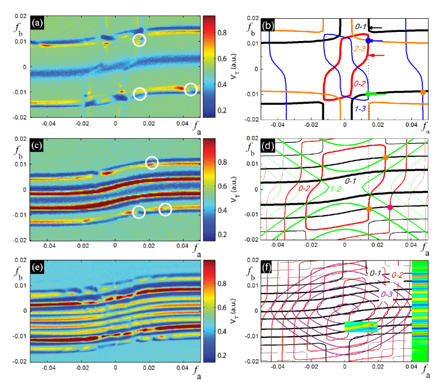
Figure 1: (Color online). Multi-photon resonances in the system of coupled flux qubits. The tank voltage amplitude (a, c, e) and the energy contour lines (b, d, f) versus the partial bias fluxes $f_{\mathrm{a}}$ and $f_{\mathrm{b}}$ for different driving frequencies (from top to bottom): $\omega/2\pi=17.6$, $7.0$, $4.1$ GHz. Numbers $k-j$ next to the lines mean that the line relates to the energy difference $E_{j}-E_{k}$. The color inset in (f) is plotted for $\lambda$, Eq. (4), by solving the Bloch-Redfield equation for the reduced density matrix.

In the left panel in Fig. 1 we present the experimental results (the voltage amplitude of the tank as a function of qubit biases) for the system of two coupled flux qubits. The driving frequency $\omega/2\pi$ is $17.6$ for (a), $7.0$ GHz for (c), and $4.1$ for (e). The system can be resonantly excited from the level $k$ to the level $j$ when the energy of $n$ photons matches them:

$$\Delta E_{kj}(f_{\mathrm{a}},f_{\mathrm{b}})\equiv E_{j}-E_{k}=n\cdot\hbar\omega.$$ (5)

Then along the contour lines defined with this relation the resonant structure appears. (Besides, the trough due to the ground state curvature is visible at the center, around $f_{\mathrm{b}}$ close to $0$.) The resonances are visualized with the ridge-trough line. However, the ridge-trough line is disturbed with increasing or decreasing the signal; some of these changes are shown with white circles. This means changing the effective Josephson inductance in these points. We argue that this happens because of the ladder-type multi-photon excitations to higher levels (see also Ref. Fink08 ).

To understand the experimental results, we plot the energy contour lines in Fig. 1(b,d,f) for three frequencies $\omega$, by making use of relation (5). Consider first Fig. 1(b). The black and red lines show the positions of the expected resonant excitations from the ground state to the first and to the second excited states respectively. The blue and orange lines are the contour lines for the possible excitations from the first and from the second excited state to the third excited state. The one-photon resonances along the black and red curves are clearly visible in Fig. 1(a); this was used for the spectroscopical study of the system Izmalkov08 . For better understanding we calculate the energy levels, by diagonalizing Hamiltonian (1), and plot them at fixed value of the bias flux through qubit $a$, $f_{\mathrm{a}}$, as a function of the bias flux through qubit $b$, $f_{\mathrm{b}}$, in Fig. 2(a); the arrows of the length $\omega/2\pi=17.6$ GHz and $7.0$ GHz (orange) are introduced to match the energy levels. The black and red arrows in both Fig. 2(a) and Fig. 1(b) show the position of one-photon transitions to the first and the second excited levels. The double green and blue arrows in Fig. 2 show the position of the two-photon processes, where the excitation by the first photon creates the population of the first and the second levels and the second photon excites the system to the upper level. We emphasize that these two-photon excitations happen via intermediate levels. The position of these expected resonances is shown in Fig. 1(b) with the blue and green thick points. Indeed, there is the change of the signal in Fig. 1(a) in these points. (The two-photon resonance $0-2-3$, shown with the blue point, was shown with the numerical simulation in Ref. th .) Moreover, the orange point in Fig. 1(b) stand for the ladder-type three-photon excitation, $0-1--3$ (with one photon to the first excited level and then with two photons to the upper level), which is also visible in Fig. 1(a).

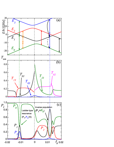
Figure 2: (Color online). Ladder-type transitions and the inverse population. (a) Energy levels of two coupled qubits at $f_{\mathrm{a}}=0.015$ versus $f_{\mathrm{b}}$ (i.e. along the dotted line in Fig. 1 (b,d)). (b) Transition matrix elements $T_{nm}$ between the eigenstates $\left|E_{m}\right\rangle$ and $\left|E_{n}\right\rangle$. (c) The energy levels occupation probabilities $P_{i}$ under driving with frequency $\omega/2\pi=17.6$ GHz.

In Fig. 1(c) we can see the ridge-trough resonances for the driving frequency $\omega/2\pi=7$ GHz. Comparing with the contour lines in Fig. 1(d) we easily notice that the resonances are one- and two-photon resonant excitations to the first excited level. Note that the two-photon resonant excitation is direct and happen without any intermediate level in contrast to the above described resonances. The higher level excitations via the first excited state appear due to three- and four-photon excitations, as shown with orange ($0--1-2$) and pink ($0--1--2$) dots in Fig. 1(d). These resonances are visible in Fig. 1(c).

In Fig. 1(e) the response of the two-qubit system is shown for $\omega/2\pi=4.1$ GHz. The lines along the horizontal axis are due to direct 1-, 2-, 3-, and 4-photon excitations to the first excited state; cf. black lines in Fig. 1(f). Numerous upper level excitations via the first excited level appear as the amplification and lowering the signal along these lines. For illustration in Fig. 1(f) beside transitions to the first excited level (black line) we plot the red and violet lines which match the ground state and the second and third excited states.

The transition probability from the state $\left|E_{m}\right\rangle$ into the state $\left|E_{n}\right\rangle$ is defined by the absolute value of the matrix element of the perturbation. From Eqs. (1-3) these are given by:

$$T_{nm} = \left|\left\langle E_{n}\right|\widehat{v}\left|E_{m}\right\rangle\right|^{2},$$ (6)

$$\widehat{v} = \frac{1}{I_{\mathrm{p}}^{(\mathrm{b})}}\left(I_{\mathrm{p}}^{(\mathrm{a})}\widehat{\sigma}_{z}^{(\mathrm{a})}+I_{\mathrm{p}}^{(\mathrm{b})}\widehat{\sigma}_{z}^{(\mathrm{b})}\right),$$

where we have divided the perturbation by the factor $I_{\mathrm{p}}^{(\mathrm{b})}\Phi_{0}\cdot f_{\mathrm{ac}}$. We plot the transition matrix elements in Fig. 2(b) to describe the ladder-type excitations shown in Fig. 1(b) with the green and blue points. The position of the respective resonances is shown in Fig. 2(a) and (b) respectively with green and blue arrows and dotted lines. In the left half of Fig. 2(b) we plot the transition elements around the transition between the three levels $E_{0}$, $E_{1}$, and $E_{3}$. In the right half we plot the transition elements related to three levels $E_{0}$, $E_{2}$, and $E_{3}$. In the latter case the transition element between the higher two levels ($E_{2}$ and $E_{3}$) is smaller than between the lower two levels ($E_{0}$ and $E_{2}$): $T_{23}\ll T_{02}$. In contrast, in the former case the transition element between the higher two levels ($E_{1}$ and $E_{3}$) is significantly larger than between the lower two levels ($E_{0}$ and $E_{1}$): $T_{13}\gg T_{01}$. Important to note that in both cases the transition element from the ground state to the highest excited level, $T_{03}$, is very small. This means that the probability of the direct excitation to the highest level is very small – the transition is induced exceptionally due to ladder-type mechanism.

And finally we calculate the energy level occupation probabilities under driving. This is done by means of the numerical solution of the Bloch-Redfield equation for the qubit system density matrix $\widehat{\rho}$ Storcz03 . The impact of the dissipative environment on the qubit system is described by the Redfield relaxation tensor. Conveniently the environment is modelled as the harmonic oscillator common bath with the ohmic spectral densities Storcz03 . Then the coupling of the qubit system to the environment is characterized with only one phenomenological parameter $\alpha$, which describes the strength of the dissipative effects. Important to note that this model accurately describes the relaxation between different levels of the systems (in contrast to the often used approach with equal relaxation rates for all energy levels), since respective relaxation rates are essentially different. Then the fitting of the experimental graphs is done with Eq. (4), where the expectation value of the current in $i$-th qubit is calculated with the reduced density matrix: $I_{\mathrm{qb}}^{(i)}=-I_{\mathrm{p}}^{(i)}Sp(\widehat{\rho}\widehat{\sigma}_{z}^{(i)})$. The result of the calculation is presented as the inset in Fig. 1(f). Such fitting gives us the parameter for the strength of dissipation $\alpha=0.1$ and the driving amplitudes $f_{\mathrm{ac}}\times 10^{3}=4,$ $6,$ and $8$ for Fig. 1(a), (c), and (e) respectively.

The numerically calculated energy level occupation probabilities are plotted in Fig. 2(c) for $\omega/2\pi=17.6$ GHz, $f_{\mathrm{ac}}=4\times 10^{-3}$, $f_{\mathrm{a}}=15\times 10^{-3}$ versus $f_{\mathrm{b}}$, that is along the dotted line in Fig. 1(b). This graph demonstrates two interesting phenomena, similar to those which exhibit atoms in the laser field Vitanov01 . First, the ladder-type resonant excitation takes place to the left, where the upper level occupation probability $P_{3}$ is of the same order as the intermediate level occupation probability $P_{1}$. This corresponds to the green point in Fig. 1(b). Second, the inverse population appears to the right (corresponds to the blue point in Fig. 1(b)). This means that the upper level occupation probability $P_{1}$ is larger than the ground state one $P_{0}$ Astafiev07 ; You07 ; Berns08 ; Sun09 . In our case the inverse population at the first excited level is accumulated after relaxation from the third excited level, since relaxation from the third level to the first one (shown with solid curved arrow in Fig. 2(a)) is larger than both relaxation from the third to second and from the first to the ground state (shown with dashed curved arrow in Fig. 2(a)).

In conclusion, the multi-photon resonances in the four-level (two flux qubit) system were observed. The multi-photon resonances were of two kinds: direct and via intermediate level (when three levels are relevant for the process). Our calculations show that in the latter case the stationary state of the system with different relaxation rates exhibits the inverse population. Such effects are relevant for both multi-photon spectroscopy of the system and for the study of new effects in artificial multi-level structures.

This work was supported by the EU through the EuroSQIP project, by the DFG project IL 150/6-1 and by Fundamental Researches State Fund grant F28.2/019. E.I. acknowledges the financial support from Federal Agency on Science and Innovations of Russian Federation under contract No. 02.740.11.5067 and the financial support from Russian Foundation for Basic Research, Grant RFBR-FRSFU No. 09-02-90419. M.G. was partially supported by the Slovak Scientific Grant Agency Grant No. 1/0096/08, the Slovak Research and Development Agency under the contract No. APVV-0432-07 and No. VCCE-005881-07, ERDF OP R&D, Project CE QUTE ITMS 262401022, and via CE SAS QUTE.

References

- (1) W.D. Oliver, Ya. Yu, J.C. Lee, K.K. Berggren, L.S. Levitov, and T.P. Orlando, Science 310, 1653 (2005).
- (2) M. Sillanpää, T. Lehtinen, A. Paila, Yu. Makhlin, and P. Hakonen, Phys. Rev. Lett. 96, 187002 (2006).
- (3) C.M. Wilson, T. Duty, F. Persson, M. Sandberg, G. Johansson, and P. Delsing, Phys. Rev. Lett. 98, 257003 (2007).
- (4) A. Izmalkov, S.H.W. van der Ploeg, S.N. Shevchenko, M. Grajcar, E. Il’ichev, U. Hübner, A.N. Omelyanchouk, and H.-G. Meyer, Phys. Rev. Lett. 101, 017003 (2008).
- (5) G. Sun, X. Wen, Y. Wang, Sh. Cong, J. Chen, L. Kang, W. Xu, Y. Yu, S. Han, and P. Wu, Appl. Phys. Lett. 94, 102502 (2009).
- (6) Y. Yu, W.D. Oliver, J.C. Lee, K.K. Berggren, L.S. Levitov, and T.P. Orlando, arXiv:cond-mat/0508587.
- (7) S.K. Dutta, F.W. Strauch, R.M. Lewis, K. Mitra, H. Paik, T.A. Palomaki, E. Tiesinga, J.R. Anderson, A.J. Dragt, C.J. Lobb, and F. C. Wellstood, Phys. Rev. B 78, 104510 (2008).
- (8) D.M. Berns, M.S. Rudner, S.O. Valenzuela, K.K. Berggren, W.D. Oliver, L.S. Levitov, and T.P. Orlando, Nature 455, 51 (2008).
- (9) Yu.A. Pashkin, T. Yamamoto, O. Astafiev, Y. Nakamura, D. V. Averin, and J. S. Tsai, Nature 421, 823 (2003).
- (10) A.J. Berkley, H. Xu, R.C. Ramos, M.A. Gubrud, F. W. Strauch, P. R. Johnson, J. R. Anderson, A. J. Dragt, C.J. Lobb, and F.C. Wellstood, Science 300, 1548 (2003).
- (11) A. Izmalkov, M. Grajcar, E. Il’ichev, Th. Wagner, H.-G. Meyer, A.Yu. Smirnov, M.H.S. Amin, A. Maassen van den Brink, and A.M. Zagoskin, Phys. Rev. Lett. 93, 037003 (2004).
- (12) J.B. Majer, F.G. Paauw, A.C.J. ter Haar, C.J.P.M. Harmans, and J.E. Mooij, Phys. Rev. Lett. 94, 090501 (2005).
- (13) R. McDermott, R.W. Simmonds, M. Steffen, K.B. Cooper, K. Cicak, K. D. Osborn, S. Oh, D.P. Pappas, and J. M. Martinis, Science 307, 1299 (2005).
- (14) A. Fay, E. Hoskinson, F. Lecocq, L.P. Levy, F.W.J. Hekking, W. Guichard, and O. Buisson, Phys. Rev. Lett. 100, 187003 (2008).
- (15) J.Q. You and F. Nori, Physics Today 58(11), 42 (2005).
- (16) G. Wendin and V.S. Shumeiko, Low Temp. Phys. 33, 724 (2007).
- (17) A. Zagoskin and A. Blais, Phys. Canada 63, 215 (2007).
- (18) T. Yamamoto, Yu. A. Pashkin, O. Astafiev, Y. Nakamura, and J. S. Tsai, Nature 425, 941 (2003).
- (19) J.H. Plantenberg, P.C. de Groot, C.J.P.M. Harmans, and J.E. Mooij, Nature 447, 836 (2007).
- (20) P.J. Leek, S. Filipp, P. Maurer, M. Baur, R. Bianchetti, J.M. Fink, M. Göppl, L. Steffen, and A. Wallraff, Phys. Rev. B 79, 180511(R) (2009).
- (21) S. Rebić, J. Twamley, and G. J. Milburn, Phys. Rev. Lett. 103, 150503 (2009).
- (22) J.E. Mooij, T.P. Orlando, L. Levitov, L. Tian, C.H. van der Wal, and S. Lloyd, Science 285, 1036 (1999).
- (23) Ya.S. Greenberg, A. Izmalkov, M. Grajcar, E. Il’ichev, W. Krech, H.-G. Meyer, M.H.S. Amin, and A. Maassen van den Brink, Phys. Rev. B 66, 214525 (2002).
- (24) A.Yu. Smirnov, Phys. Rev. B 68, 134514 (2003).
- (25) S.N. Shevchenko, Eur. Phys. J. B 61, 187 (2008).
- (26) M. Grajcar, A. Izmalkov, S.H.W. van der Ploeg, S. Linzen, E. Il’ichev, Th. Wagner, U. Hübner, H.-G. Meyer, A. Maassen van den Brink, S. Uchaikin, and A.M. Zagoskin, Phys. Rev. B 72, 020503(R) (2005).
- (27) S.N. Shevchenko, S.H.W. van der Ploeg, M. Grajcar, E. Il’ichev, A.N. Omelyanchouk, and H.-G. Meyer, Phys. Rev. B 78, 174527 (2008).
- (28) M. Grajcar, S.H.W. van der Ploeg, A. Izmalkov, E. Il’ichev, H.-G. Meyer, A. Fedorov, A. Shnirman, and G. Schön, Nature Phys. 4, 612 (2008).
- (29) J.M Fink, M. Göppl, M. Baur, R. Bianchetti, P.J. Leek, A. Blais, and A. Wallraff, Nature 454, 315 (2008).
- (30) M.J. Storcz and F.K. Wilhelm, Phys. Rev. A 67, 042319 (2003).
- (31) N.V. Vitanov, T. Halfmann, B.W. Shore, and K. Bergmann, Annu. Rev. Phys. Chem. 52, 763 (2001).
- (32) O. Astafiev, K. Inomata, A.O. Niskanen, T. Yamamoto, Yu.A. Pashkin, Y. Nakamura, and J.S. Tsai, Nature 449, 588 (2007).
- (33) J.Q. You, Yu-xi Liu, C.P. Sun, and F. Nori, Phys. Rev. B 75, 104516 (2007).